New Market Opportunities and Consumer Heterogeneity in the U.S. Organic Food Market

Abstract

This paper investigates what factors and characteristics of organic consumers affect annual organic food expenditure by using Nielsen’s consumer panel dataset from 2010 to 2014. To be specific, this paper explores new marketing opportunities by investigating organic consumer heterogeneity in different household income levels by utilizing the multilevel model. Findings in this study will contribute to the previous and existing literature in three-folds. First, we find that the organic consumers are more heterogeneous in the high-level of income groups (approximately above $60,000), as well as the low-income households between $35,000 and $45,000. This finding demonstrates that the income levels above $60,000 and around $40,000 have potential market segmentation. Second, we find that that annual organic expenditure is positively associated with consumers who consecutively repurchase organic food products compared to irregular organic consumers, supporting a different level of satisfaction. Third, we find that USDA organic labeling has a positive effect on annual organic expenditure compared to the organic labeling certified by private companies, implying the importance of credibility for the organic labeling.

1. Introduction

According to the Organic Trade Association (OTA), the total U.S. organic sales and growth increased continuously from 2006 to 2015 (Figure 1). Notably, the total organic sales in 2015 are reported $43.3 billion, 11% higher than sales in 2014 (https://www.ota.com/news/press-releases/19031). Considering the overall food consumption per year is limited, the increase in organic food sales indicates the decrease in the share of conventional food in the food market. In this regard, the organic food market has more marketing opportunities compared to the traditional food market. Organic consumers are expected to have different motivations or characteristics compared to traditional consumers. In other words, new marketing opportunities can be derived from currently growing the organic market by segmenting based on the motivations or characteristics of organic consumers.

Due to the rapidly growing demand for organic food products, abundant research has examined consumer motivations of organic food and attitude towards it. Chinnici et al. [1], Hughner et al. [2], Schifferstein and Ophuis [3], and Zanoli and Naspetti [4] review the previous studies on consumer motivations for buying organic food and find that the main motivations to consume organic food are strongly related to health and the environmental consideration compared to conventional food. It is due to the facts that consumers have a belief that organic food is more nutritious than conventional food [5,6,7]. Furthermore, the indiscriminate use of chemicals and pesticides used for conventional food production has been significantly connected with environmental deterioration [8] and human health outcomes such as a short-term headache, cancer, reproduction, and endocrine disruption [9,10,11]. Another strong motivation, the taste of organic food, is identified by a few studies. Bryła [12], Chryssochoidis [13], and Lea and Worsley [14], for example, show that the taste of organic food is a crucial factor to consume organic products because consumers perceive that organic food has better taste than conventional food. Fillion and Arazi [15] also find that tastes of organic orange juice are better than conventional orange juice. Last but not least, several important motivations, animal welfare and supporting local economies, influence the organic food purchasing attitudes [10] and quality of the product [8,16,17].

An increasing body of literature is focusing on the determinants of organic food demand or expenditure documents that income is mainly suggested as the primary driver to explain the organic food demand or expenditure. Although income is a key factor, there are mixed findings of the relationship between the income and organic food demand or expenditure. Beckmann et al. [18], Durham [19], Grunert and Kristensen [20], and Li et al. [21] show the insignificant effect of income on demand/willingness to pay/probability of purchasing organic food. On the other hand, results of Chen et al. [22], Dimitri and Dettmann [23], Jörgensen [24], and Menghi [25] show the positive effect of income on the consumption of organic food. The contradictory results of the income effect on organic food consumption indicate that the impact of income on organic food consumption is still ambiguous.

This study assumes that the existence of consumer heterogeneity might explain the ambiguous results of the income effect on organic food expenditure according to different household income levels. Cicia et al. [26] mention the organic food consumption is based on the heterogeneous preference for foods. Moreover, Thiele and Weiss [27] find that the household income has a positive impact on the choice of food varieties with ascending order of income. It is therefore essential to identify the heterogeneity of organic food consumers and explore new marketing opportunities for organic food in already matured U.S. organic food market.

The primary objective of this paper is to investigate the possible organic consumer heterogeneity according to different household income levels by utilizing Nielsen’s consumer panel data from 2010 to 2014. Specifically, this study tries to focus on the organic market segmentation, since the U.S. organic markets have matured with the rapid growth in organic sales. The multilevel model allows for the segmenting of the organic food market based on household income heterogeneity. Employing the multilevel model also makes a difference for our study compared to previous and existing studies that investigate the probability of buying organic products [19], or estimate the likelihood of market participation and consumption level by focusing a specific category of organic products [28,29,30]. A multilevel model is estimated that accounts for the possibility of consumer heterogeneity at different income levels while controlling for unobservable heterogeneity in household income effects on organic food expenditures (One way to control the unobservable individual characteristics or motivations about organic food could be the fixed effect model (FE) or random effect model (RE). However, the variation of the marginal income effect in each household is difficult to capture using FE or RE). A further expansion is to include USDA labeling as knowledge/awareness of organic foods. Gifford and Bernard [31], Krystallis and Chryssohoidis [32], and Li et al. [21] argue that knowledge of organic food is an important factor for purchasing behavior of organic food. This study hypothesizes that organic consumers tend to buy more organic products with USDA labeling compared to other third party organic labeling services due to the lack of knowledge and credibility. Additionally, we examine the overall satisfaction between two groups of organic consumers by hypothesizing that annual organic expenditure is influenced by repurchasing organic consumers than irregular organic consumers. Previous studies such as Chinnici et al. [1], Grunert [33], and LaBarbera and Mazursky [34] find that repurchasing behavior of organic food is strongly correlated with satisfaction. In this regard, we impose a strong assumption that consumers who are satisfied with previous organic food consumption consequently result in forming a repurchase intention for organic food.

2. Data

This study uses Nielsen Company’s consumer panel data to estimate U.S. organic food expenditure (The Nielsen company’s consumer panel data is provided by James M, Kilts Center for Marketing at Chicago Booth and Nielsen Company. More information about Nielsen consumer panel can be found at http://research.chicagobooth.edu/nielsen/). The Nielsen Marketing Data is composed of the consumer panel and retail scanner data. The consumer panel data consists information about product purchases made by a panel of consumer households across all retail outlets in all U.S. markets including food, non-food grocery items, health and beauty aids, and select general merchandise. The data contains 40,000 to 60,000 U.S. households per year. On the other hand, the retail scanner data includes weekly purchases and pricing data generated from participating retail store point-of-sale systems in all U.S. markets. Consumer panel data is the primary source of data for this study since the consumer panel dataset contains detailed demographic information for households, not in the retail scanner data (Both datasets could be combined based on uniquely assigned household ID. However, combining the two datasets results in missing observations.). An annual consumer panel is utilized from 2010 to 2014, to analyze the recent trends in organic food consumption. This study uses annual data due to the difficulty of capturing the income variation in weekly or monthly data compared to annual data. Additionally, we focus only on organic consumers by excluding non-organic consumers who never purchased organic food in our data period (Before we exclude non-organic consumers, we find that the proportion of organic households out of total sample are 49.79% in 2010, 51.70% in 2011, 51.17% in 2012, 50.90% in 2013, and 48.65% in 2014, respectively. This implies that about 50% of respondents in Nielsen consumer panel purchase organic products at least one time in a year). The exclusion allows for marketing opportunities for the mature U.S. organic market to explored [35]. After selecting households who purchase organic food at least once between 2010 and 2014, we have an unbalanced yearly panel of households from 2010 to 2014, with a total of 154,308 observations. On an annual basis, the number of observations is 30,194, 32,100, 30,973, 31,097, and 29,944, respectively (Additionally, we looked at the total quantity consumed in each year to illustrate the buying patterns of organic households. The total quantity consumed for the organic products are 572,021 in 2010, 662,203 in 2011, 660,304 in 2012, 685,645 in 2013, and 574,984 in 2014, respectively).

Table 1. Descriptive Summary Statistics (N = 154,308).

Variable	Type	Description	Mean	Std. Dev	Exp. Sign
Expenditure	Continuous	Total annual organic expenditure (in logs)	3.09	1.52
Income	Continuous	Average annual income (in thousands)	70.38	31.41	+
Black	Binary	1 if HH is Black/African American; 0 otherwise	0.07	0.25	−
Asian	Binary	1 if HH is Asian; 0 otherwise	0.04	0.20	−
Other	Binary	1 if HH is Other; 0 otherwise	0.05	0.21	−
Household Size	Continuous	Number of individuals residing in the home	2.87	1.19	+
College	Binary	1 if education level of HH is some college; 0 otherwise	0.30	0.46	+
Graduate	Binary	1 if education level of HH is college or post-college graduate; 0 otherwise	0.44	0.50	+
Age1	Binary	1 if age of HH is between 30 and 49; 0 otherwise	0.35	0.48	+/−
Age2	Binary	1 if age of HH is between 50 and over 65; 0 otherwise	0.63	0.48	+/−
Children6	Binary	1 if HH has children with less than age 6; 0 otherwise	0.04	0.20	+
Middle Atlantic	Binary	1 if region is Middle Atlantic; 0 otherwise	0.13	0.33	+/−
East North	Binary	1 if region is East North Central; 0 otherwise	0.18	0.38	+/−
West North	Binary	1 if region is West North Central; 0 otherwise	0.08	0.27	+/−
South Atlantic	Binary	1 if region is South Atlantic Central; 0 otherwise	0.20	0.40	+/−
East South	Binary	1 if region is East South Central; 0 otherwise	0.06	0.23	+/−
West South	Binary	1 if region is West South Central; 0 otherwise	0.10	0.30	+/−
Mountain	Binary	1 if region is Mountain; 0 otherwise	0.08	0.27	+/−
Pacific	Binary	1 if region is Pacific; 0 otherwise	0.13	0.34	+/−
Married	Binary	1 if HH is married; 0 otherwise	0.01	0.08	−
USDA	Binary	1 if USDA organic seal on product; 0 otherwise	0.70	0.46	+
Repurchase	Binary	1 if HH consumes organic food at least one consecutive year; 0 otherwise	0.27	0.45	+

Notes: HH represents the head of the household. Middle Atlantic includes New Jersey, New York, and Pennsylvania. East North Central includes Indiana, Illinois, Michigan, Ohio, and Wisconsin. West North Central includes Iowa, Kansas, Minnesota, Missouri, Nebraska, North Dakota, and South Dakota. South Atlantic includes Delaware, District of Columbia, Florida, Georgia, Maryland, North Carolina, South Carolina, Virginia, and West Virginia. East South Central includes Alabama, Kentucky, Mississippi, and Tennessee. West South Central includes Arkansas, Louisiana, Oklahoma, and Texas. Mountain includes Arizona, Colorado, Idaho, New Mexico, Montana, Utah, Nevada, and Wyoming. Pacific includes Alaska, California, Hawaii, Oregon, and Washington. Finally, our reference category of New England includes Connecticut, Maine, Massachusetts, New Hampshire, Rhode Island, and Vermont.

shows descriptive summary statistics with the expected signs for all variables used in this analysis.

For income, the expected sign on organic expenditure is positive unless organic food is found to be an inferior good. In the original consumer panel dataset, the income variable is composed of 16 different categories. However, the income effect on organic expenditure is expected to be different based on each household’s income level. It is because the household income has a hierarchical order of positive effect on the food varieties as income increases [27]. For this reason, the income variable is converted to a continuous variable by using the average to capture variations in different income categories. For example, if income category for household i is between $5000 and $7000, the income value of $6000 is assigned to the household i. Other demographic and socioeconomic variables are included in this study. The variable of children under six is created as a dummy variable because it is expected to be positively associated with organic expenditures since parents are more likely to consume organic food if they have young children [36,37]. All the race dummy variables are expected to be unknown compared to the based group, white (i.e., Caucasian), due to the unknown preference of organic food in each ethnic group. The level of education is hypothesized to be positively associated with organic expenditure. This is because the majority of previous studies find that consumers with a higher level of education tend to buy more organic products compared to consumers with a lower level of education [38,39,40,41]. The head of household age is expected to be unknown since there is no clear evidence of a relationship between age and organic food consumption. This study incorporates nine different regional dummies including a base region, which is the New England region, to control regional heterogeneity, and an expected sign of regional dummy variables are unknown. For marital status, this study cannot expect estimated signs for married households whether they consume more or less organic food than married households since there is no clear logic to explain relationships. According to Thompson [42], for example, the Hartman group find more willingness to purchase organic foods in the married people; whereas the results of Groff et al. [43] show that the marital status does not statistically influence organic food consumption. For the variable of USDA, households are expected to consume more if USDA organic labeling is attached to organic products compared to the labeling certified by third parties (i.e., private companies). This is because consumers might have different perception regarding the labeling of organic products based on the origin of the certificate. According to Li et al. [21], the effect of USDA organic labeling on total expenditure is expected to be high compared to the third party organic labeling due to the relatively high awareness of USDA labeling (According to the USDA, the USDA organic seal is defined as an official mark of the USDA Agricultural Marketing Service (AMS)), and it was first published with the implementation of the National Organic Program that was established in 2000. (Please see more detail about the USDA organic seal at https://www.ams.usda.gov/sites/default/files/media/Using%20the%20Organic%20Seal%20Factsheet.pdf). Nielsen consumer panel dataset includes the following information: “organic claim description” and “organic seal description.” In this study, we defined the USDA organic labeling if and only if “organic seal description = “USDA Organic Seal”. Additionally, the proportions of households with USDA organic seal based on “organic seal description” are 71.65% in 2010, 71.19% in 2011, 72.61% in 2012, and 73.75% in 2014, respectively.

Although the variable of income is the primary variable of interest in this study, we incorporate a variable called “repurchase” represented as a dummy variable with the following hypothesis: Total expenditure of organic food is more likely to be influenced by repurchase consumers than others with a single purchase. Chinnici et al. [1], Grunert [20], and LaBarbera and Mazursky [34] document that repurchasing behavior of organic food is strongly correlated with satisfaction. In other words, if consumers are satisfied with the consumption of organic foods from their previous purchase, then those consumers are more likely to repurchase organic food next time. In this regard, we include the variable of repurchase as a proxy for the satisfaction of consumer for organic food by imposing a strong assumption that household i are satisfactory for organic food if he/she consecutively more consumes the organic food from the previous period. Also, we consider the consumption difference between t and t − 1 because there might exist consumers who buy organic products with curiosity. Thus, the variable of repurchase takes on the value of 1 if household i consumes organic food in current year consecutively from the previous year and if their quantity consumed in time t is greater than or equal to the quantity consumed at time t − 1. Since several studies such as Dynan [44] and Fuhrer [45] assert that the current consumption is significantly affected by previous consumption, we expect the variable of repurchase is positively associated with organic expenditure.

3. The Empirical Model

This study employs a multilevel model framework focusing on the effect of organic consumer heterogeneity on organic expenditure rather than the choice of organic or conventional foods. Additionally, a multilevel model has the following econometric advantages. First, the clustering means covariate in the multilevel model allows to control potential endogeneity issues in level 2, the household characteristics in this study [46]. Secondly, capturing the random errors in the level 2 allows for the estimation of differences of coefficients in level 2. Third, fixed effect estimators used in multilevel models are unbiased even though there exists multicollinearity in level 1 [47]. Fourth, the multilevel model allows for the control of sample selection bias. Grilli and Rampichini [46] find that the unbiased estimators are obtained by utilizing a multilevel model even though the unobserved factors exist either at the higher or lower level.

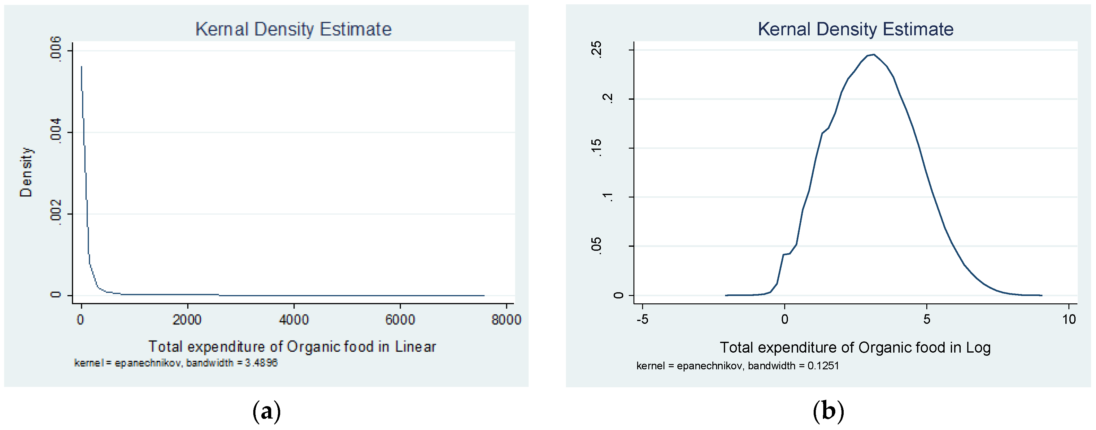
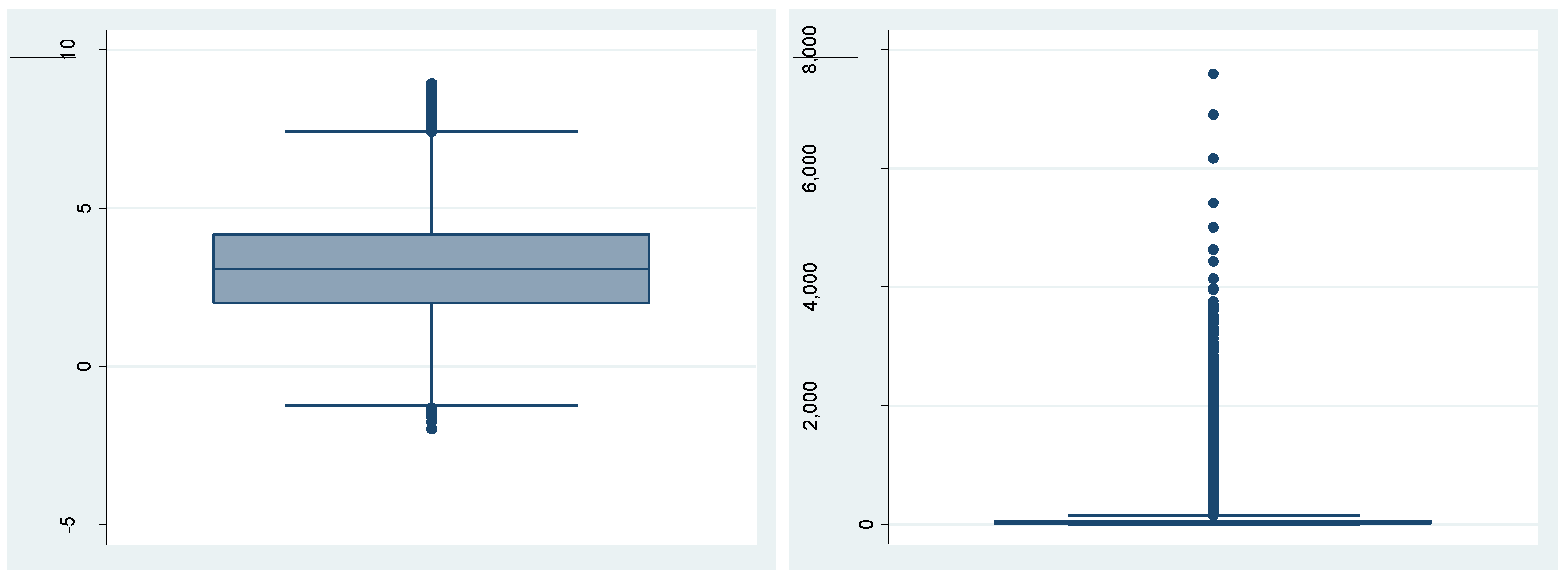
The multilevel model is estimated with a log-linear functional form for two reasons. First, the log transformation of the dependent variable is more amenable to interpreting the elasticity as the percent change. Second, this paper uses the box-and-whisker plots and the univariate kernel density estimation to select the functional form for the dependent variable. Figure 2 shows the difference between linear and log dependent variables, and we find that the distribution of a log dependent variable (b) is closer to normal distribution compared to the linear dependent variable (a). Also, Figure 3 shows the results of box-and-whisker between the two functional forms (linear and log) of the dependent variable. We find that there are more outliers in the linear functional form compared to the log transformation of the dependent variable. More outliers infer a higher variance and consequently result in a heteroscedasticity problem [48].

Before we estimate the multilevel model, we test multicollinearity based on Variance Inflation Factor (VIF) whether two or more of independent variables are strongly correlated or not, and we find there is no firm evidence of multicollinearity (i.e., VIF < 10). Finally, the log-linear multilevel model is specified by the following equation:

$$\begin{array}{l}\ln {(OrganicExpenditure)}_{it}\\ ={\pi }_{i0}+{\pi }_{i1}\ln {(C\_Income)}_{it}+{\beta }_{02}Repurchas{e}_{it}+{\beta }_{03}Repurchas{e}_{it}\\ +{\beta }_{04}Ed{u}_{it}+{\beta }_{05}Ag{e}_{it}+{\beta }_{06}Chil{d}_{it}+{\beta }_{07}Rac{e}_{it}+{\beta }_{08}USD{A}_{it}\\ +{\beta }_{09}Regio{n}_{it}+{\beta }_{10}Marrie{d}_{it}+{\epsilon }_{it}\end{array}$$

(1)

where i is the level 2 (household), t is the level 1 (year), C_Income_it = Income_it − $\overline{{\mathit{Income}}_i}$, π_i0 = β₀₀ + δ_i0, and π_i1 = β₀₁ + δ_i1.

By substituting π_i0 and π_i1, Equation (1) can be rewritten as:

$$\begin{array}{l}\ln {(OrganicExpenditure)}_{it}\\ =({\beta }_{00}+{\delta }_{i0})+({\beta }_{01}+{\delta }_{i1})\ln {(C\_Income)}_{it}+{\beta }_{02}Repurchas{e}_{it}\\ +{\beta }_{03}Repurchas{e}_{it}+{\beta }_{04}Ed{u}_{it}+{\beta }_{05}Ag{e}_{it}+{\beta }_{06}Chil{d}_{it}+{\beta }_{07}Rac{e}_{it}\\ +{\beta }_{08}USD{A}_{it}+{\beta }_{09}Regio{n}_{it}+{\beta }_{10}Marrie{d}_{it}+{\epsilon }_{it}\end{array}$$

(2)

By clustering random and fixed parts, Equation (2) can be rearranged into the following equation:

$$\begin{array}{l}\ln {(OrganicExpenditure)}_{it}\\ ={\beta }_{00}+{\beta }_{01}\ln {(C\_Income)}_{it}+{\beta }_{02}Repurchas{e}_{it}+{\beta }_{03}Repurchas{e}_{it}\\ +{\beta }_{04}Ed{u}_{it}+{\beta }_{05}Ag{e}_{it}+{\beta }_{06}Chil{d}_{it}+{\beta }_{07}Rac{e}_{it}+{\beta }_{08}USD{A}_{it}\\ +{\beta }_{09}Regio{n}_{it}+{\beta }_{10}Marrie{d}_{it}+{\delta }_{i0}+{\delta }_{i1}\ln {(C\_Income)}_{it}+{\epsilon }_{it}\end{array}$$

(3)

where ${\beta }_{00}$ denotes the intercept; ${\beta }_{01}$, ${\beta }_{02}$, ${\beta }_{03}$, ${\beta }_{04}$, ${\beta }_{05}$, ${\beta }_{06}$, ${\beta }_{07}$, ${\beta }_{08}$, ${\beta }_{09}$, and ${\beta }_{10}$ represent the level-1 estimators; ${\delta }_{i0}$, ${\delta }_{i1}$, and ${\epsilon }_{it}$ are the error terms. In detail, ${\delta }_{i0}$ represents the level 2 error variance in the intercept and ${\delta }_{i1}$ is the level 2 residual variance in the level-1 slope of $\ln {\left(C\_Income\right)}_{it};$ ${\epsilon }_{it}$ represents the entire model’s errors subtracting the level-2 variances.

The primary difference between the multilevel model and OLS regression model is the error terms. The regression model has only one error term whereas the multilevel model divides a single error term into three with level 1, level 2, and variance-covariance in level 2. For a hierarchy framework, there are assumptions made about the disturbances. Based on Steenbergen and Jones [49], the five assumptions, which are common in multilevel models, are imposed in this analysis. The first assumption is no systematic parameter noise or level-1 noise, and this can be defined as $E\left[{\delta }_{i0}\right]=E\left[{\delta }_{i1}\right]=E\left[{\epsilon }_{it}\right]=0$. The second assumption is $\mathrm{Var}\left[{\delta }_{i0}\right]={\tau }_0{\tau }_0$, $\mathrm{Var}\left[{\delta }_{i1}\right]= {\tau }_1{\tau }_1$, $\mathrm{Var}\left[{\epsilon }_{it}\right]={\delta }^2$. Since the multilevel model estimators are estimated based on these variance components, all disturbance terms are assumed a constant variance in level-1 and level-2. The third assumption, which is defined as $Cov\left[{\delta }_{i0}, {\delta }_{i1}\right] ={\tau }_0{\tau }_1$, comes from a correlation between the level-2 disturbances on the intercepts and slopes. In general, the level-2 units with small slope have small intercept or large slope have large intercept conversely, and the covariance term ${\tau }_0{\tau }_1$ captures the relationship between the intercepts and slopes. The fourth assumption is that ${\delta }_{i0}$ and ${\delta }_{i1}$ are assumed to be normally distributed similar to the ${\epsilon }_{it}$. Combining all four assumptions above, the level-1 disturbances from a normal distribution are distributed with mean 0 and variance ${\delta }^2$, and the level-2 disturbances from a bivariate normal distribution are distributed with mean 0 and variance-covariance matrix is defined as following: $\sum = \left(\begin{array}{c}{\tau }_0{\tau }_0 {\tau }_0{\tau }_1\\ {\tau }_1{\tau }_0 {\tau }_1{\tau }_1\end{array}\right)$. The final assumption of $Cov\left[{\delta }_{i0}, {\epsilon }_{it}\left] = Cov\right[ {\delta }_{i1}, {\epsilon }_{it}\right] = 0$ indicates that the errors between level-1 unit on the dependent variable, and the location of slopes and intercepts are uncorrelated.

This paper employs the log-likelihood test to evaluate the usage of a multilevel model compared to a single-level regression. The null hypothesis of the log-likelihood test is that there is no significant difference between the two models. Therefore, the multilevel model specification can be justified as a proper model compared to the single-level model based on the log-likelihood test result.

4. Results

Table 2. Results of Random Effects Test.

	Without Centering	With Centering
Random Effect Parameters	Estimate	Estimate
Constant	1.2359	1.2077
	(0.0128)	(0.0042)
Income	0.008	0.009
	(0.0004)	(0.0005)
Correlation	−0.3516	−0.0322
	(0.0248)	(0.0265)
Std. deviation (Residual)	0.7315	0.7287
	(0.0017)	(0.0017)
Log-Likelihood Ratio Test for Multilevel Model vs. Linear Regression
Chi-square	80,735.42	82,698.12
p-value	0.0000	0.0000

Note: Standard errors are reported in parentheses.

represents the results of random effects test including models with a centering (cluster mean covariate method accounting for endogeneity) and without centering. The random effect parameters show the variance and covariance matrix for intercept and income. Based on the results of the log-likelihood ratio test, this study finds that the multilevel model specification is better than the single-level regression model by rejecting the null hypothesis that single-level regression model is preferred to the multilevel model specification.

Table 3. Results of Multilevel Models with and without Centering.

	Without Centering			With Centering
Variable	Coef.		SE	Coef.		SE
Income	0.006	***	0.0001	−		−
Centered Income	−		−	0.001	***	0.0002
Black	−0.146	***	0.0200	−0.137	***	0.0202
Asian	0.201	***	0.0265	0.234	***	0.0267
Others	0.044	**	0.0216	0.031	*	0.0187
Household Size	0.004		0.0036	0.009	***	0.0036
College	0.205	***	0.0110	0.252	***	0.0111
Graduate	0.396	***	0.0120	0.503	***	0.0118
Age30_49	−0.162	***	0.0231	−0.103	***	0.0234
Age49_over	−0.287	***	0.0237	−0.235	***	0.0240
Children6	0.235	***	0.0162	0.227	***	0.0163
Middle Atlantic	−0.226	***	0.0279	−0.229	***	0.0281
East North	−0.401	***	0.0267	−0.434	***	0.0269
West North	−0.515	***	0.0298	−0.553	***	0.0302
South Atlantic	−0.273	***	0.0263	−0.299	***	0.0265
East South	−0.527	***	0.0316	−0.586	***	0.0320
West South	−0.334	***	0.0286	−0.355	***	0.0289
Mountain	0.013		0.0297	−0.025		0.0301
Pacific	0.268	***	0.0279	0.260	***	0.0282
Married	0.006		0.0170	0.045	***	0.0271
USDA	0.052	***	0.0053	0.054	***	0.0052
Repurchase	0.822	***	0.0047	0.825	***	0.0047
Constant	2.335	***	0.0384	2.785	***	0.0382
Log-likelihood	−228,981.32			−229,748.25
AIC	458,014.60			459,548.50
BIC	458,273.30			459,807.10
Observations	154,308			154,308

Notes: Significance levels are indicated by *, **, and *** for 10, 5, and 1 percent significance level, respectively. SE is a standard error. AIC and BIC represent Akaike Information Criterion and Bayesian Information Criterion, respectively.

shows the results of multilevel models with centering and without centering. Since the mean centering method can control the potential endogeneity problem in level 2 [46], the model with centering is our benchmark model. In Table 3, most of the estimated signs are consistent with our expected signs presented in Table 1. Compared to white households, Asian households consume about 23 percent more on organic food whereas black households spend 13.7 percent less. For different levels of education, this paper finds that households who have college graduate or higher degrees of education consume more organic food compared to those who have a high school diploma or less. This finding could be explained that advanced degrees lead to higher income and better knowledge about potential health outcomes to purchase organic (The mean difference in annual income between households with high school or less and other is approximately $20,000).

Nine different regional dummies are included to control for the possible regional heterogeneity. Interestingly, households in the Pacific region consume more organic food than New England, and this finding is consistent with our expectation in that the majority certified acres of organic farmland are located in the Pacific region according to USDA Economic Research Service (https://www.ers.usda.gov/data-products/organic-production/). The other seven regions consume less organic food relative to New England. This result may reflect that the overall income level in coastal areas in the U.S. is relatively higher than in other regions based on our data. As of 2017, the total estimated population of all coastal states was 252,771,773, which is approximately 77.7% of the total U.S. population. Furthermore, this study finds if households are married, then they consume more organic food than households who are single including widowed and divorced households.

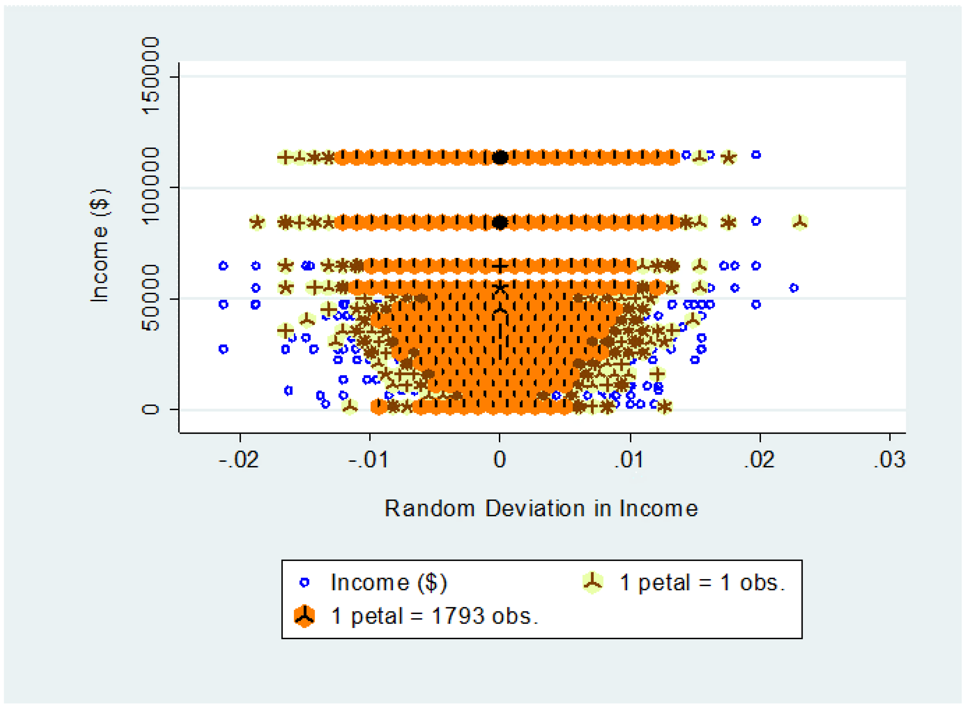
For income, which is one of our primary variables of interest, this study finds that income has a statistically significant impact on annual organic expenditure. Based on an estimated coefficient of centered income, on average, $1000 increases in annual income will result in increasing annual organic food expenditure by 0.1%, ceteris paribus. Figure 4 shows the sunflower plots between the deviation in income coefficient and income level based on results from the post-estimation. This paper utilizes sunflower plots rather than scatter plots since sunflower plots are useful to display high-density bivariate data [50]. Since we have many observations for each household income level, sunflower plots are helpful to understand the shape of distribution for the deviations in income coefficient along with the different income levels. Specifically, the Figure 4 represents how each household’s income level deviates from the average income coefficient (${\beta }_{01})$ where 1 petal equals 1793 observations. As shown in Figure 4, the deviations from the average income effects are overall increasing as income increases, except for the interval between $40,000 and $50,000. One possible explanation might be explained by Supplemental Nutrition Assistance Program (SNAP) that allows the low-income households to buy organic food. This also support the less heterogeneity (i.e., narrower distribution) in the group of the low-income households.

In addition to the main variable of interest, household income, this study finds that organic products labeling certified by USDA is associated with a 0.6% increase in annual organic food expenditure compared to the organic products certified by third parties (i.e., private companies). This finding implies that consumers have different attitudes toward organic products based on labeling, even though the products are the same as organic. Furthermore, we find that the total expenditure of organic food is positively associated with repurchasing consumers compared to consumers who consume organic food irregularly. This finding could be explained by Díaz et al. [51] in that frequent organic consumers are more willing to pay a premium price for organic good compared to other groups of consumers. Thus, there is a need to create and develop current marketing strategies to satisfy consumers for increasing sales from current organic consumers and to attract new customers.

4.1. Comparison with the Previous Findings

Compared to the previous studies on organic expenditure, the factors used in this study to explain organic expenditure are consistent with the most previous studies. To be specific, the variable of white is consistent with Alviola and Capps [28] and Dimitri, M. Venezia, and States [52] who show that white households are the least likely to consume organic milk compared to other races. According to the positive impact of education, this result is supported by similar findings in Sandalidou et al. [53] and Yue et al. [54]. The negative impact of age on organic expenditure is consistent with Detre et al. [55] in that they find that Millennial-aged students are more likely buy organic produce. Additionally, Govindasamy et al. [56] find that respondents who are over the age of 50 consume organic products 17 percent less than younger counterparts. Although most of the variables in this study show similar results with the previous studies, we find that the deviations from the average income effects differ from Thiele and Weiss [27] who show that the positive income effect on consumers’ choice of food varieties with ascending order. Our finding, however, shows that the variations of income effect are wider in high-income households (more than $60,000), implying that high-income households may have a desire for a variety of organic foods compared to the low-income households.

4.2. Robustness Tests

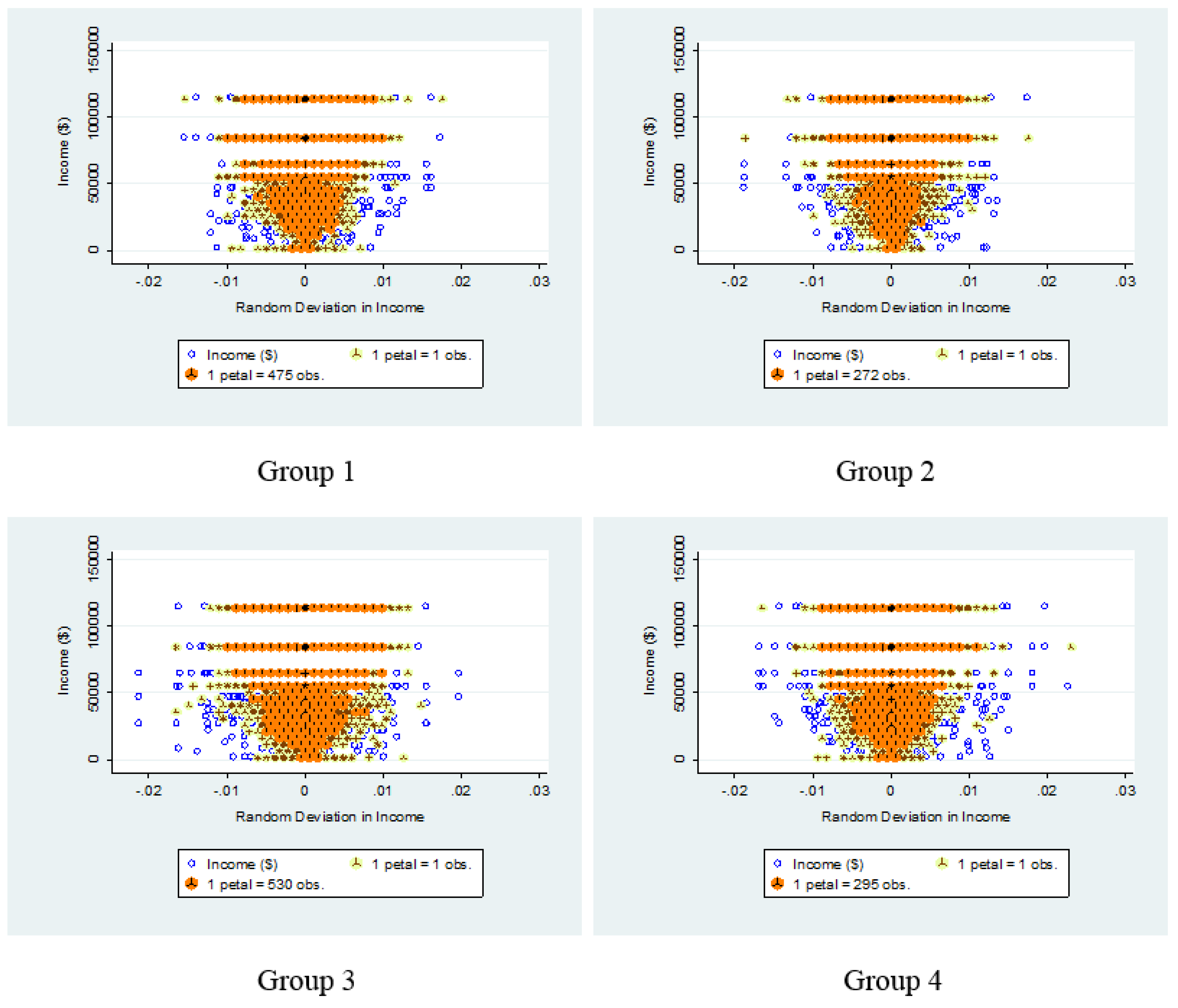
This paper conducts several robustness tests. First, we estimate different functional forms between log-linear and linear-linear, and we find that all estimated coefficients in our benchmark model, which is log-linear functional form, are robust with linear-linear functional form (Results with different functional forms are not provided but can be provided upon reviewer’s request.). Second, we divide our sample into four different subgroups based on state income levels and re-produce the sunflower distributions for the four different groups (Our sample is divided by following two steps. First, we split states of the U.S. based on the U.S. median household income during 2010–2014. Second, states above the U.S. median household income are divided above and below 50%. Similarly, states below the U.S. median household income are divided above and below 50% (see

Table A1. Income per Capita and Median Household Income by States (2010–2014).

Ranking	State	Income Per Capita	Median Household Income	Group
1	Maryland	36,338	73,971	1
2	Massachusetts	36,593	71,919	1
3	District of Columbia	45,877	71,648	1
4	Alaska	33,062	71,583	1
5	Connecticut	39,373	70,048	1
6	Hawaii	29,736	69,592	1
7	New Jersey	37,288	69,160	1
8	New Hampshire	34,691	66,532	1
9	Virginia	34,052	64,902	1
10	California	30,441	61,933	1
11	Minnesota	32,638	61,481	1
12	Washington	31,841	61,366	2
13	Colorado	32,357	61,303	2
14	Utah	24,877	60,922	2
15	Delaware	30,488	59,716	2
16	North Dakota	33,071	59,029	2
17	New York	33,095	58,878	2
18	Illinois	30,417	57,444	2
19	Wyoming	29,698	57,055	2
20	Rhode Island	30,830	54,891	2
21	Vermont	29,178	54,166	2
22	Iowa	28,361	53,712	2
23	Pennsylvania	29,220	53,234	3
24	Texas	27,125	53,035	3
25	Nebraska	27,446	52,686	3
26	Wisconsin	28,213	52,622	3
27	Kansas	27,870	52,504	3
28	Nevada	25,773	51,450	3
29	Oregon	27,646	51,075	3
30	South Dakota	26,959	50,979	3
31	Arizona	25,715	50,068	3
32	Michigan	26,613	49,847	3
33	Maine	27,978	49,462	3
34	Indiana	25,140	49,446	3
35	Georgia	25,615	49,321	3
36	Ohio	26,937	49,308	3
37	Missouri	26,126	48,363	3
38	Idaho	23,938	47,861	4
39	Oklahoma	25,229	47,529	4
40	Florida	26,582	47,463	4
41	North Carolina	25,774	46,556	4
42	Montana	25,989	46,328	4
43	South Carolina	24,596	45,238	4
44	New Mexico	23,683	44,803	4
45	Louisiana	24,800	44,555	4
46	Tennessee	24,922	44,361	4
47	Kentucky	23,684	42,958	4
48	Alabama	23,606	42,830	4
49	Arkansas	22,883	41,262	4
50	West Virginia	22,714	41,059	4
51	Mississippi	21,036	39,680	4
Median	United States	28,889	53,657

Source: 2010–2014 American Community Survey 1-Year Estimates.

). Figure 5 shows the sunflower distributions of four different groups, and we find that the shapes of the distributions in Figure 5 are similar with Figure 4, except group 2 in that the deviation of the income effect is lower in group 2 compared to other groups, especially income interval between $20,000 and $40,000. Furthermore, the deviations of income effect for the high-income households are not significantly different according to Figure 5.

Third, we estimate the multilevel model with mean centering for the four different subgroups separately based on state income levels.

Table 4. Robustness Test with Four Different Income Groups.

	Group 1		Group 2		Group 3		Group 4
Variable	Coef.		Coef.		Coef.		Coef.
Income	0.0005		0.0008		0.0010	**	0.0012	**
	(0.0005)		(0.0006)		(0.0005)		(0.0006)
Black	−0.2077	***	0.0241		−0.1343	***	−0.2042	***
	(0.0443)		(0.0564)		(0.0375)		(0.0413)
Asian	0.1002	**	0.2932	***	0.2374	***	0.3036	***
	(0.0435)		(0.0651)		(0.0573)		(0.0811)
Others	−0.0068		0.1017	**	−0.0022		0.0235
	(0.0373)		(0.0482)		(0.0360)		(0.0449)
Household Size	0.0290	***	0.0022		0.0080		−0.0083
	(0.0082)		(0.0091)		(0.0065)		(0.0087)
College	0.2538	***	0.2324	***	0.2593	***	0.2653	***
	(0.0283)		(0.0309)		(0.0206)		(0.0255)
Graduate	0.5368	***	0.5579	***	0.5280	***	0.4882	***
	(0.0289)		(0.0315)		(0.0214)		(0.0266)
Age30_49	−0.1171	**	−0.0034		−0.1072	**	−0.1456	**
	(0.0553)		(0.0622)		(0.0429)		(0.0572)
Age49_over	−0.2590	***	−0.1470	**	−0.2342	***	−0.2922	***
	(0.0566)		(0.0637)		(0.0440)		(0.0581)
Children6	0.2198	***	0.1765	***	0.2253	***	0.2836	***
	(0.0374)		(0.0438)		(0.0298)		(0.0411)
Married	−0.0037		0.0415		0.0691	**	−0.0006
	(0.0359)		(0.0414)		(0.0317)		(0.0410)
USDA	0.0476	***	0.0731	***	0.0564	***	0.0705	***
	(0.0122)		(0.0134)		(0.0096)		(0.0126)
Repurchase	0.7830	***	0.8038	***	0.8281	***	0.8747	***
	(0.0104)		(0.0118)		(0.0085)		(0.0116)
Constant	2.8581	***	2.5897	***	2.6130	***	2.8072	***
	(0.0742)		(0.1085)		(0.0926)		(0.0861)
Log-Likelihood	−40,264.576		−33,642.183		−70,179.851		−42,002.553
Observation	27,423		22,609		46,616		27,716

Notes: Significance levels are indicated by **, and *** for 10, 5, and 1 percent significance level, respectively. Standard errors are reported in parentheses.

shows the results of the multilevel model for four different subgroups with the mean centering. By comparing the four models with our benchmark model in Table 3, we find that the estimated signs and coefficients of our benchmark model are robust with the results of the four models. However, the primary variable, income, is only robust with the last two models. To be specific, the income variable is found insignificant in group 1 and 2 that state income levels are above the U.S. median income level, implying that consumers living in high-income states do not statistically influence total organic expenditure. This finding could be supported by the facts that the share of high-income households is very high in the high-income states compared to the low-income states. Furthermore, the insignificant income effect could be explained by a lack of accessibility. Even though households have a high income, total organic expenditure might not be significantly affected if they have a lack of accessibility to purchase organic food.

5. Conclusions

This paper investigates what factors and characteristics of organic consumers affect annual organic food expenditure by using Nielsen’s consumer panel dataset from 2010 to 2014. To be specific, this paper explores new marketing opportunities by investigating organic consumer heterogeneity in different income levels utilizing the multilevel model. Although there is abundant literature on consumers’ consumption of organic foods, our findings fill in a gap by providing implications and contributions to the existing literature on organic expenditures. First, our findings show that the organic consumers are more heterogeneous in the high-level of income groups (approximately above $60,000) due to the broader deviations of the household income effect. One possible marketing strategy for the high-income group of households is that retailers should open exclusive organic food outlets, such as Fresh Market. Another possible strategy could be developing diverse organic products since the desire for the number of organic offerings is increasing in the income level. For low-income customers (approximately between $35,000 and $45,000), we find that the deviations are narrower (i.e., households are less heterogeneous) than the high-income group but increasing along with the income level. Thus, we suggest that the possible marketing strategy for the low-income customers (approximately between $35,000 and $45,000) is to enlarge the existing organic food sections in the grocery stores regarding diversity. One possible marketing strategy for the low-income households is giving promotional information to the low-income households rather than high-income households. This is because low-income households are more sensitive to the price of organic products compared to the high-income households. Another possible strategy is to enroll more organic foods in the food stamp program, also known as Supplemental Nutrition Assistance Program (SNAP). Since SNAP provides a monthly supplement for buying nutritious food especially to low-income families, low-income consumers can access more the organic food by enrolling the food stamp. Second, the proxy variable of the consumer satisfaction for organic foods, repurchase, is positively associated with organic food expenditure. It is an important finding since the organic food market in the U.S. has matured. However, most of the previous studies have focused on the relationship between satisfaction and organic food purchase intention or between organic food attributes and organic food purchase intention. Thus, our results suggest that previous studies should be expanded to investigate the repurchase behavior rather than purchase behavior for organic food. It is because the relative importance of factors to repurchase intention for organic food may be different with factors to purchase intention. The positive effect of the repurchase variable, a proxy for the satisfaction of organic products, on organic expenditure implies the importance of consumer management. Considering the matured organic markets in the U.S., managers in grocery stores need to develop such a customer care program or sales/marketing management to manage the existing organic customers, as well as inducing new potential organic consumers. Third, we find that USDA organic labeling has a positive effect on annual organic expenditure compared to the organic labeling certified by private companies. This finding implies that the signaling effect from the different labeling results in a different impact on organic expenditure even though they provide the same information as organic products. Also, organic consumers might have a stronger perception of USDA labeling than third-party organic products due to the credibility. To compete with the USDA labeling, third-party auditors and food companies should address additional information about awareness and credibility, in addition to their basic food safety and nutrition concerns of the organic food products. For example, increasing portion of the package most likely to be seen by customers at the time of purchase by including ingredient state and other product information might help to increase organic sales.

This study can be extended in four different ways. First, the level of consumer satisfaction might vary based on different time dimension, which can be justified based on the subject of the researcher and the primary purpose of the research. Therefore, monthly or weekly data with a different methodology could be employed to investigate and capture the different level of the satisfaction in organic food for the future study. However, it will be challenging especially in the field experiment compared to survey method to match income data up with a disaggregated variable. Second, this study can be extended by dividing organic foods into specific categories because consumers might have a different level of satisfaction in different categories of organic food. Third, determinants of the significant deviations for income effect in low-income states compared to high-income states could be investigated to understand aspects of organic consumers. Forth, investigating the factors that explain the different effects of certification between USDA and third parties might expand organic market sizes or shares in the U.S.

References

- Chinnici, G.; D’Amico, M.; Pecorino, B. A Multivariate Statistical Analysis on the Consumers of Organic Products. Br. Food J. 2002, 104, 187–199. [Google Scholar] [CrossRef]
- Hughner, R.S.; McDonagh, P.; Prothero, A.; Shultz, C.J., II; Stanton, J. Who Are Organic Food Consumers? A Compilation and Review of Why People Purchase Organic Food. J. Consum. Behav. 2007, 6, 94–110. [Google Scholar] [CrossRef]
- Schifferstein, H.N.J.; Peter, A.M. Oude Ophuis. Health-Related Determinants of Organic Food Consumption in The Netherlands. Food Qual. Pref. 1998, 9, 119–133. [Google Scholar] [CrossRef]
- Zanoli, R.; Naspetti, S. Consumer Motivations in the Purchase of Organic Food: A Means-End Approach. Br. Food J. 2002, 104, 643–653. [Google Scholar] [CrossRef] [Green Version]
- Baker, S.; Thompson, K.E.; Engelken, J.; Huntley, K. Mapping the Values Driving Organic Food Choice: Germany vs the UK. Eur. J. Mark. 2004, 38, 995–1012. [Google Scholar] [CrossRef]
- Hill, H.; Lynchehaun, F. Organic Milk: Attitudes and Consumption Patterns. Br. Food J. 2002, 104, 526–542. [Google Scholar] [CrossRef]
- Lockie, S.; Lyons, K.; Lawrence, G.; Grice, J. Choosing Organics: A Path Analysis of Factors Underlying the Selection of Organic Food among Australian Consumers. Appetite 2004, 43, 135–146. [Google Scholar] [CrossRef] [PubMed]
- Rana, J.; Paul, J. Consumer Behavior and Purchase Intention for Organic Food: A Review and Research Agenda. J. Retailing Consum. Serv. 2017, 38, 157–165. [Google Scholar] [CrossRef]
- Baldi, I.; Filleul, L.; Mohammed-Brahim, B.; Fabrigoule, C.; Dartigues, J.; Schwall, S.; Drevet, J.; Salamon, R.; Brochard, P. Neuropsychologic Effects of Long-Term Exposure to Pesticides: Results from the French Phytoner Study. Environ. Health Perspect. 2001, 109, 839–844. [Google Scholar] [CrossRef] [PubMed] [Green Version]
- Boockmann, B.; Fries, J.; Göbel, C. Specific Measures for Older Employees and Late Career Employment. 2012. Available online: https://papers.ssrn.com/abstract=2159817 (accessed on 31 May 2017).[Green Version]
- Rivas, A.; Cerrillo, I.; Granada, A.; Mariscal-Arcas, M.; Olea-Serrano, F. Pesticide Exposure of Two Age Groups of Women and Its Relationship with Their Diet. Sci. Total Environ. 2007, 382, 14–21. [Google Scholar] [CrossRef] [PubMed]
- Bryła, P. Organic food consumption in Poland: Motives and barriers. Appetite 2016, 105, 737–746. [Google Scholar] [CrossRef] [PubMed]
- Chryssochoidis, G.M. Testing and Validating the LOV Scale of Values in an Organic-Food-Purchase-Context. In World Scientific Book Chapters; World Scientific Publishing Co. Pte. Ltd.: Singapore, 2004; pp. 291–301. Available online: https://ideas.repec.org/h/wsi/wschap/9789812796622_0018.html (accessed on 1 May 2018).
- Lea, E.; Worsley, T. Australians’ Organic Food Beliefs, Demographics and Values. Br. Food J. 2005, 107, 855–869. [Google Scholar] [CrossRef]
- Fillion, L.; Arazi, S. Does Organic Food Taste Better? A Claim Substantiation Approach. Nutr. Food Sci. 2002, 32, 153–157. [Google Scholar] [CrossRef]
- Bryła, P. The perception of EU quality signs for origin and organic food products among Polish consumers. Qual. Assur. Saf. Crops Foods 2017, 9, 345–355. [Google Scholar] [CrossRef]
- Lucas, M.R.; Röhrich, K.; Marreiros, C.; Fragoso, R.; Kabbert, R.; Clara, A.M.; Martins, I.; Böhm, S. Quality, Safety and Consumer Behaviour towards Organic Food; CEFAGE-UE Working Paper 5; CEFAGE-UE: Évora, Portugal, 2008. [Google Scholar]
- Beckmann, S.C.; Brokmose, S.; Lind, R.L. Danske Forbrugere og Økologiske Fødevarer: ØKO Foods II Projektet; Handelshøjskolens Forlag: Oslo, Norway, 2001. [Google Scholar]
- Durham, C. Organic Purchase Dedication: A Fractional Probit Model. Agric. Resour. Econ. Rev. 2007, 36, 304–320. [Google Scholar] [CrossRef]
- Grunert, S.C.; Kristensen, K. Den Danske Forbruger og Økologiske Fødevarer; Institut for Informationsbehandling, Handelshøjskolen i Århus: Aarhus, Denmark, 1992. [Google Scholar]
- Li, J.; Zepeda, L.; Gould, B.W. The Demand for Organic Food in the U.S.: An Empirical Assessment. J. Food Distrib. Res. 2007, 38, 1–16. [Google Scholar]
- Chen, B.; Saghaian, S.; Zheng, Y. Organic Labelling, Private Label, and US Household Demand for Fluid Milk. Appl. Econ. 2018, 50, 3039–3050. [Google Scholar] [CrossRef]
- Dimitri, C.; Dettmann, R.L. Organic Food Consumers: What Do We Really Know about Them? Br. Food J. 2012, 114, 1157–1183. [Google Scholar] [CrossRef]
- Jörgensen, C. Prisbildning Och Efterfrågan På Ekologiska Livsmedel; Livsmedelsekonomiska Institutet (SLI): Stockholm, Sweden, 2001. [Google Scholar]
- Menghi, A. Consumer Response to Ecological Milk in Sweden; Examensarbete-SLU; Institutionen Foer Ekonomi: Uppsala, Sweden, 1997. [Google Scholar]
- Cicia, G.; del Giudice, T.; Scarpa, R. Consumers’ Perception of Quality in Organic Food: A Random Utility Model under Preference Heterogeneity and Choice Correlation from Rank-Orderings. Br. Food J. 2002, 104, 200–213. [Google Scholar] [CrossRef]
- Thiele, S.; Weiss, C. Consumer Demand for Food Diversity: Evidence for Germany. Food Policy 2003, 28, 99–115. [Google Scholar] [CrossRef]
- Alviola, P.A.; Capps, O. Household Demand Analysis of Organic and Conventional Fluid Milk in the United States Based on the Nielsen Homescan Panel. Agribusiness 2010, 26, 369–388. [Google Scholar] [CrossRef]
- Smed, S. Information and consumer perception of the “organic” attribute in fresh fruits and vegetables. Agric. Econ. 2012, 43, 33–48. [Google Scholar] [CrossRef]
- Zhang, F.; Huang, C.L.; Lin, B.H.; Epperson, J.E. Modeling fresh organic produce consumption with scanner data: A generalized double hurdle model approach. Agribusiness 2008, 24, 510–522. [Google Scholar] [CrossRef]
- Gifford, K.; Bernard, J.C. The Impact of Message Framing on Organic Food Purchase Likelihood. J. Food Distrib. Res. 2004, 35, 19–28. [Google Scholar]
- Krystallis, A.; Chryssohoidis, G. Consumers’ Willingness to Pay for Organic Food: Factors That Affect It and Variation per Organic Product Type. Br. Food J. 2005, 107, 320–343. [Google Scholar] [CrossRef]
- Grunert, K.G. Current Issues in the Understanding of Consumer Food Choice. Trends Food Sci. Technol. 2002, 8, 275–285. [Google Scholar] [CrossRef]
- LaBarbera, P.A.; Mazursky, D. A Longitudinal Assessment of Consumer Satisfaction/Dissatisfaction: The Dynamic Aspect of the Cognitive Process. J. Mark. Res. 1983, 20, 393–404. [Google Scholar] [CrossRef]
- Von Meyer-Höfer, M.; Olea-Jaik, E.; Padilla-Bravo, C.A.; Spiller, A. Mature and Emerging Organic Markets: Modelling Consumer Attitude and Behaviour with Partial Least Square Approach. J. Food Prod. Mark. 2015, 21, 626–653. [Google Scholar] [CrossRef]
- Davies, A.; Titterington, A.J.; Cochrane, C. Who Buys Organic Food: A Profile of the Purchasers of Organic Food in Northern Ireland. Br. Food J. 1995, 97, 17–23. [Google Scholar] [CrossRef]
- Yiridoe, E.K.; Bonti-Ankomah, S.; Martin, R.C. Comparison of Consumer Perceptions and Preference toward Organic versus Conventionally Produced Foods: A Review and Update of the Literature. Renew. Agric. Food Syst. 2005, 20, 193–205. [Google Scholar] [CrossRef]
- Nasir, V.A.; Karakaya, F. Consumer Segments in Organic Foods Market. J. Consum. Mark. 2014, 31, 263–277. [Google Scholar] [CrossRef]
- Onyango, B.M.; Hallman, W.K.; Bellows, A.C. Purchasing Organic Food in US Food Systems: A Study of Attitudes and Practice. Br. Food J. 2007, 109, 399–411. [Google Scholar] [CrossRef]
- Roitner-Schobesberger, B.; Darnhofer, I.; Somsook, S.; Vogl, C.R. Consumer Perceptions of Organic Foods in Bangkok, Thailand. Food Policy 2008, 33, 112–121. [Google Scholar] [CrossRef]
- Zepeda, L.; Li, J. Characteristics of Organic Food Shoppers. J. Agric. Appl. Econ. 2007, 39, 17–28. [Google Scholar] [CrossRef]
- Thompson, G.D. Consumer Demand for Organic Foods: What We Know and What We Need to Know. Am. J. Agric. Econ. 1998, 80, 1113–1118. [Google Scholar] [CrossRef]
- Groff, A.J.; Kreider, C.R.; Toensmeyer, U.C. Analysis of the Delaware Market for Organically Grown Produce. J. Food Distrib. Res. 1993, 24, 118–126. [Google Scholar]
- Dynan, K.E. Habit Formation in Consumer Preferences: Evidence from Panel Data. Am. Econ. Rev. 2000, 90, 391–406. [Google Scholar] [CrossRef]
- Fuhrer, J.C. Habit Formation in Consumption and Its Implications for Monetary-Policy Models. Am. Econ. Rev. 2000, 90, 367–390. [Google Scholar] [CrossRef]
- Grilli, L.; Rampichini, C. Selection Bias in Linear Mixed Models. Metron Int. J. Stat. 2010, 68, 309–329. [Google Scholar] [CrossRef]
- Shieh, Y.-Y.; Fouladi, R.T. The Effect of Multicollinearity on Multilevel Modeling Parameter Estimates and Standard Errors. Educ. Psychol. Meas. 2003, 63, 951–985. [Google Scholar] [CrossRef]
- Kim, G.; Schieffer, J.; Mark, T. Do Superfund Sites Affect Local Property Values? Evidence from a Spatial Hedonic Approach; Agricultural and Applied Economics Association: Washington, DC, USA, 2016; Available online: http://ageconsearch.umn.edu/bitstream/235835/2/Revised%202016%20AAEA%20Paper%20(GwanSeon%20Kim).pdf (accessed on 1 March 2017).
- Steenbergen, M.R.; Jones, B.S. Modeling Multilevel Data Structures: EBSCOhost. Am. J. Political Sci. 2002, 46, 218–237. [Google Scholar] [CrossRef]
- Dupont, W.D.; Plummer, W.D., Jr. Density Distribution Sunflower Plots in Stata 8. In Proceedings of the 3rd North American Stata Users Group Meeting, Boston, MA, USA, 23–24 August 2004. [Google Scholar]
- Díaz, F.J.M.; Pleite, F.M.-C.; Paz, J.M.M.; García, P.G. Consumer Knowledge, Consumption, and Willingness to Pay for Organic Tomatoes. Br. Food J. 2012, 114, 318–334. [Google Scholar] [CrossRef]
- Dimitri, C.; Venezia, K.M. Retail and Consumer Aspects of the Organic Milk Market; USDA: Washington, DC, USA, 2007.
- Sandalidou, E.; Baourakis, G.; Siskos, Y. Customers’ Perspectives on the Quality of Organic Olive Oil in Greece: A Satisfaction Evaluation Approach. Br. Food J. 2002, 104, 391–406. [Google Scholar] [CrossRef]
- Yue, C.; Grebitus, C.; Bruhn, M.; Jensen, H.H. Potato Marketing–Factors Affecting Organic and Conventional Potato Consumption Patterns. In Proceedings of the 12th Congress of the European Association of Agricultural Economists–EAAE, Ghent, Belgium, 26–29 August 2008; Available online: http://ageconsearch.umn.edu/bitstream/43948/2/149.pdf (accessed on 1 August 2017).
- Detre, J.D.; Mark, T.B.; Clark, B.M. Understanding Why College-Educated Millennials Shop at Farmers’ Markets: An Analysis of Students at Louisiana State University. J. Food Distrib. Res. 2010, 41, 14–24. [Google Scholar]
- Govindasamy, R.; DeCongelio, M.; Italia, J.; Barbour, B.; Anderson, K. Empirically Evaluating Consumer Characteristics and Satisfaction with Organic Products. New Jersey Agricultural Experiment Station P-02139-1-01. 2001. Available online: http://ageconsearch.tind.io/record/36736/files/pa010101.pdf (accessed on 1 May 2017).
Figure 1.
Total U.S. Organic Sales and Growth, 2006–2015. Source: Organic Trade Association (https://www.ota.com/news/press-releases/19031).
Figure 2.
Compare between linear and log dependent variable based on Kernel Density Estimate.
Figure 3.
Comparison between Linear and Log Dependent Variable based on Box Plots.
Figure 4.
Sunflower Plots for Random Deviation in Income Coefficient.
Figure 5.
Sunflower Plots for Random Deviation from Income Coefficient by State Income Groups.