Investigations on the Coregistration of Sentinel-1 TOPS with the Conventional Cross-Correlation Technique

Abstract

In Sentinel-1 TOPS mode, the antenna sweeps in the azimuth direction for the purpose of illuminating the targets with the entire azimuth antenna pattern (AAP). This azimuth sweeping introduces an extra high-frequency Doppler term into the impulse response function (IRF), which poses a more strict coregistration accuracy for the interferometric purpose. A 1/1000 pixel coregistration accuracy is required for the interferometric phase error to be negligible, and the enhanced spectral diversity (ESD) method is applied for achieving such accuracy. However, since ESD derives miscoregistration from cross-interferometric phase, and phase is always wrapped to $[-\pi ,\pi )$, an initial coregistration method with enough accuracy is required to resolve the phase ambiguity in ESD. The mainstream for initial coregistration that meets this requirement is the geometrical approach, which accuracy mainly depends on the accuracy of orbits. In this article, the authors propose to investigate the feasibility of using the conventional coregistration approach, namely the cross-correlation-and-rigid-transformation, as the initial coregistration method. The aim is to quantify the coregistration accuracy for cross-correlation-and-rigid-transformation using the Cramér-Rao lower bound (CRLB) and determine whether this method could eventually help to resolve the phase ambiguities of ESD. In addition, we studied the feasibility and robustness of the cross-correlation plus ESD under different conditions. For validation, we checked whether the cross-correlation plus ESD approach could reach the same coregistration accuracy as geometrical plus ESD approach. In general, for large areas with enough coherence and little topography variance, the cross-correlation method could be used as an alternative to the geometrical approach. The interferogram from the two different approaches (with ESD applied afterward) shows a negligible difference under such circumstances.

1. Introduction

Coregistration is one of the important steps in SAR interferometry (InSAR). Coregistration means that the single look complex (SLC) images must be “aligned” well so that the they could be compared pixel-wise for differences, where the differences reveal ground information such as height or movement. The miscoregistration will cause coherence loss in the interferogram for stripmap mode [1]. Common stripmap product requires a coregistration accuracy of around 0.1 pixel to avoid non-negligible decorrelation [1].

Then, in 2006, De Zan [2] proposed the Terrain Observation by Progressive Scans (TOPS) mode as a successor to the ScanSAR as the new wide swath mode. Similar to the ScanSAR mode, the TOPS also operates in the burst mode for gaining a wider range scanning area. The difference between the ScanSAR and the TOPS mode is that, in the TOPS mode, the antenna “sweeps” in the azimuth direction in each subswath so that all targets are scanned by the entire azimuth antenna pattern (AAP), and the scalloping effect is minimized when comparing with the ScanSAR mode [2]. This new acquisition mode was firstly tested on the German satellite TerraSAR-X for validation [3,4,5]. Then in 2014, the Sentinel-1 (S1) mission made TOPS famous by setting it as the default acquisition mode and making the data free to the public. Every design aspects of S1 TOPS mode is aimed at doing interferometry and time series analysis [6,7]. For example, the twin satellites, S1A & S1B, have minimum six-day revisit time and a 200 m tube orbit control [8,9]. What’s more important, S1 has a routine acquisition that covers almost the whole earth, which means a rich archived dataset almost anywhere on earth. The popularity of S1 TOPS mode has drawn great attention to studying its interferometric capability.

However, coregistration for TOPS mode has a much stricter requirement than stripmap. In TOPS mode, the sweeping of antenna introduces a quadratic doppler frequency in azimuth that exceeds the pulse repetition frequency (PRF). For “aligning” this high-frequency quadratic phase term, a very high coregistration accuracy is required. A miscoregistration will not only cause decorrelation, but will also introduce a phase bias [3,10] into the interferometric product. To avoid introducing non-negligible phase error into the interferogram, a coregistration accuracy of 0.001 pixel is required [10]. For such reasons, it is important to exploit the suitable coregistration methods for TOPS that meets the 0.001 pixel accuracy requirement.

There are mainly three ways of doing coregistration: cross-correlation-and-rigid-transformation (from now on referred to as “cross-correlation method”) [11], geometrical approach [12] and (enhanced) spectral diversity [3,13]. Cross-correlation method firstly estimates shifts between master and slave image at different locations. Then a rigid transformation is performed for slave image based on the estimated shifts (or sometimes a non-linear transformation, but the discussion throughout this study will be limited to rigid transformation due to the small orbit crossing angle of TOPS. This will also be discussed in Section 2.1). Then, in recent years, with the improving quality of satellite orbital state vectors, the geometrical approach has been brought to the table. This approach could be seen as a mapping from SAR coordinates to Cartesian coordinates with the help of very precise orbits and digital elevation model (DEM). The coregistration accuracy for this approach mainly depends on the accuracy of orbital state vectors (it also depends on the topography, e.g., an available SRTM; but due to the very small orbital crossing angle of S1, the impact of topography to the final coregistration accuracy is very small and SRTM is already good enough for that [3,14]. Details are given in Section 2.2). With the availability of precise orbital state vectors for S1 with an accuracy of 5 cm [15], this approach is accepted by the current SAR community as the initial coregistration method. Meanwhile, neither of the two aforementioned methods could guarantee to reach the required 0.001 pixel coregistration accuracy in azimuth direction for TOPS [10]. Thus, after the initial coregistration, the enhanced spectral diversity (ESD) method [3,13] is applied to correct the residual coregistration error and achieve the coregistration requirement for TOPS. ESD has been proved to be quite robust in most of the stationary scenes [10].

ESD compares the phase differences of two images. The azimuth miscoregistration is derived from this differential phase. Since ESD operates on phase, one should always note the wrapped nature of phase. This means that an as-precise-as-possible initial coregistration should be performed so that the differential phase in ESD step is limited to $[-\pi ,\pi )$. Below, it is shown that the $[-\pi ,\pi )$ in ESD is equivalent to a 0.05 pixel accuracy for avoiding phase ambiguity. The current trend for TOPS is the geometrical coregistration followed by ESD (from now on referred to as “established approach”) when the precise orbits are available. On the other side, the cross-correlation method followed by ESD (from now on referred to as “proposed approach”) is rarely studied and discussed for S1 TOPS case. In this study, we want to explore the feasibility of using the proposed approach, to understand if there are some special processing steps related to the proposed approach, and to determine if and when the proposed approach could be used as an alternative to the established approach with a negligible discrepancy. In fact, the features of S1 system, such as the small temporal baseline (six days for S1A-S1B or twelve days for S1A-S1A and S1B-S1B), small spatial baseline (120∼200 m tube [8]) and small orbital crossing angle (<0.001° [14]), are all in favor of the cross-correlation method, as the quality of cross-correlation and estimation depends on good coherence and all the merits of S1 significantly reduce the temporal and geometrical decorrelation.

For a comprehensive understanding of the proposed approach, we carry out this study in two aspects: (1) to understand the coregistration accuracy of the cross-correlation method; and (2) to evaluate if the proposed approach (cross-correlation method followed by the ESD) could give identical interferogram with the established approach.

Specifically, for evaluating the theoretical coregistration accuracy of the cross-correlation method, we use Cramér-Rao lower bound (CRLB) to show the lower bound on the coregistration accuracy. For validating the accuracy of the cross-correlation method, we read the miscoregistration error from the cross-interferogram phase in the ESD step. For verifying the correctness of the proposed approach with respect to the established approach, we compare the interferograms from the two approaches, and check if there is a non-negligible phase difference.

This article is organized as follows. Section 2 discusses the theoretical coregistration accuracy of the two methods, the cross-correlation method and the geometrical method, using the idea of CRLB. Section 3 briefly describes the ESD method. Section 4 experiments on real data for a variety of different cases. There are two purposes for running experiments. The first one is to validate the coregistration accuracy of the cross-correlation method by looking at the cross-interferogram. The second purpose is to check for interferogram phase difference between the proposed approach and the established approach. In the last sections, we discuss a few points regarding the proposed approach, such as the topography, the orbital crossing angle and temporal baseline.

2. The Coregistration Accuracy of Cross-Correlation Method and Geometrical Method

2.1. Cross-Correlation and Rigid-Transformation

The problem of coregistration is very similar to the time delay estimation (TDE) problem in signal processing [16,17]. In sequence, the cross-correlation method does the following:

• Performs the cross-correlation between master and slave image using small windows at different locations;
• Performs the maximum likelihood estimation (MLE) on the cross-correlation between master and slave windows to estimate the offsets;
• Estimates the transformation matrix for the slave image based on the calculated offsets at different locations; and
• Performs the rigid transformation based on the estimated transformation matrix.

In the steps above, two estimations are performed. The first estimates the offsets for small windows between master and slave at different locations. The second estimates the transformation matrix. The two estimations accuracy will be discussed separately.

2.1.1. The Accuracy of Estimating Offsets

Several patches distributed uniformly on master and slave images are selected for estimating the offsets. A patch is usually a small square window of the size n. When $n=1$, the patch is a point. For each patch, the offset is estimated with MLE after cross-correlation. Now we express this process in a mathematical way. Suppose there is a mutual shift between the master and slave patch, denoted as the following:

$$\begin{array}{cc}\hfill u_1[n]& =s[n]+w_1[n],\hfill \end{array}$$

(1)

$$\begin{array}{cc}\hfill u_2[n]& =\alpha s[n-\Delta n]+w_2[n],n=1,\dots ,N\hfill \end{array}$$

(2)

$$\begin{array}{cc}\hfill \gamma & =\frac{E[u_1{u}_2^{\ast }]}{\sqrt{E[{|u_1|}^2]E[{|u_2|}^2]}}\hfill \end{array}$$

(3)

where $u_1[n]$ is the master signal, $u_2[n]$ is the slave signal with offset $\Delta n$, $\ast$ is the conjugation operator, $s[n]$ is the signal, $w[n]$ is the speckle noise in SAR imagery, $\alpha$ is the amplitude gain; $\gamma$ is the coherence which is also related to the signal clutter ratio (SCR), N is the size of the patch, and $\Delta n$ is the mutual shift for this patch that needs to be estimated. Note that in general $u_1$ and $u_2$ are complex signals and the cross-correlation is carried out in the complex domain [18]. In several studies $w[n]$ is assumed as the complex, zero mean stationary white noise, and then $u_i[n]$ is referred as the stationary circular Gaussian process [19,20]. In the following discussion, the analysis is carried out for the 1D signals as in Equations (1) and (2) but the conclusions could also be expanded to the 2D case.

The MLE of the cross-correlation between $u_1$ and $u_2$ gives an estimated mutual shift value denoted as $\Delta \widehat{n}$. The CRLB of $\Delta \widehat{n}$ is [19,21]:

$${\sigma }_{\Delta \widehat{n}}=\sqrt{\frac{3}{2N}}\frac{\sqrt{1-{\gamma }^2}}{\pi \gamma }$$

(4)

The reason for using the CRLB is because the MLE is asymptotically unbiased and efficient. Here, the CRLB could also be expressed as a function of SCR. It is assumed that the master and slave patches have close enough SCR, where the SCR is defined as:

$$\mathrm{SCR}=\frac{{\sigma }_s^2}{{\sigma }_w^2}$$

(5)

${\sigma }_s^2$ and ${\sigma }_w^2$ are the variances of signal and noise in Equations (1) and (2). Then, by the definition of coherence in Equation (3), supposing that $w_i[n]$ are uncorrelated zero mean complex Gaussian noise [19,20], and that $s[n]$ and $w[n]$ are also uncorrelated, then, by the definition of coherence, one would have the following [22,23]:

$$\gamma =\frac{{\sigma }_s^2}{{\sigma }_s^2+{\sigma }_w^2}=\frac{1}{1+1/\mathrm{SCR}}$$

(6)

Then Equation (4) becomes

$${\sigma }_{\Delta \widehat{n}}=\sqrt{\frac{3}{2N}}\frac{\sqrt{1+2\mathrm{SCR}}}{\pi \mathrm{SCR}}$$

(7)

When the estimation uses strong point scatterers (characterized by sufficiently high SCR values), the lower bound becomes [18,24]:

$${\sigma }_{\Delta \widehat{n},point}=\frac{\sqrt{3}}{\pi }\sqrt{\frac{1}{\mathrm{SCR}}}$$

(8)

Comparing with Equation (7), the $\sqrt{N}$ in the denominator is not there due to the central limit theorem. For strong point scatterers, $\mathrm{SCR}\gg 1$, so that $\sqrt{1+2\mathrm{SCR}}/\mathrm{SCR}\approx \sqrt{2}·\sqrt{1/\mathrm{SCR}}$.

It can be seen from both Equations (4) and (8) that, the key factor for estimation accuracy is the coherence/SCR. To obtain a higher accuracy in estimating the offsets, patches with higher SCR should be prioritized. The size of the patch is also important; however, it follows the reciprocal of square root, which means when N is large enough then increasing the patch size will not decrease CRLB significantly.

2.1.2. The Accuracy of Estimating Transformation Matrix

Now we evaluate the accuracy for the rigid transformation step. Suppose now the offsets for a number of points (or patches) have been calculated and denoted as $\Delta {\widehat{n}}_1,\dots ,\Delta {\widehat{n}}_m$. At this point, we could use again the MLE to estimate the coefficients of the rigid transformation for the slave image. The 2D slave image in vector form is ${\mathbf{S}}_{\mathbf{2}\times \mathbf{M}}$ where M is the number of points to be transformed; the linear transformation matrix is ${\mathbf{D}}_{\mathbf{2}\times \mathbf{2}}$; the translation matrix is ${\mathbf{t}}_{\mathbf{2}\times \mathbf{1}}$; and the resampled slave image is ${\tilde{\mathbf{S}}}_{\mathbf{2}\times \mathbf{M}}$. Then the rigid transform is expressed in the following way:

$${\tilde{\mathbf{S}}}_{\mathbf{2}\times \mathbf{M}}={\mathbf{D}}_{\mathbf{2}\times \mathbf{2}}·{\mathbf{S}}_{\mathbf{2}\times \mathbf{M}}+{\mathbf{t}}_{\mathbf{2}\times \mathbf{1}}\otimes {\mathbf{1}}_{\mathbf{2}\times \mathbf{M}}$$

(9)

where ${\tilde{\mathbf{S}}}_{\mathbf{2}\times \mathbf{M}}$ is the resampled slave image, ⊗ is the Kronecker product, and ${\mathbf{1}}_{\mathbf{2}\times \mathbf{M}}$ is a vector with all ones. A different way of writing the transformation function without using vectors is given in [11]. Equation 9 will have the following effects to the resampled slave image [11]:

• The Kronecker product term represents a mutual shift (on azimuth and range) between master and slave image. In InSAR, this shift is mainly due to orbital timing error (azimuth) and perpendicular baseline component (range);
• The transformation matrix D_2×2 could include a stretch in range and a rotation that skews both azimuth and range.

To understand the accuracy of the rigid transformation, we focus on the accuracy regarding the mutual shift and the rotation. The two cases could be representative for SAR image coregistration and are enough for understanding the rigid transformation accuracy in terms of CRLB. Detail regarding a more general case could be found in [25].

For the case of a mutual shift between master and slave image, suppose there are M points/patches used for the estimation, each has an estimated offset with variance ${\sigma }_{\Delta \widehat{n}}^2$. Since the M points/patches do not overlap, it is safe to assume that they are independent, and thus the estimated offsets $\Delta {\widehat{n}}_i$ are mutually independent. The CRLB for estimating the mutual shift is thus given by [25]:

$${\sigma }_{\tilde{\mathbf{S}},\mathrm{shift}}=\frac{1}{\sqrt{M}}{\sigma }_{\Delta \widehat{n}}$$

(10)

It can be seen from Equation (10) that the lower bound is independent of the locations of the points. In addition, Equation (10) applies to both range and azimuth direction.

Now we evaluate the CRLB for estimating the rotation matrix. Although in SAR coregistration, the rotation angle is very small [11], it is shown below that it does have non-negligible effects on TOPS coregistration. With the assumption that the variance for each point on the range and azimuth directions are the same, the following simplified CRLB could be derived [26]:

$${\sigma }_{\tilde{\mathbf{S}},\mathrm{rot}}=\frac{1}{\sqrt{{\sum }_{i=1}^M(s_{ix}^2+s_{iy}^2)}}{\sigma }_{\Delta \widehat{n}}$$

(11)

where $s_{ix}$ and $s_{iy}$ are the coordinates for the $i^{th}$ point in ${\mathbf{S}}_{\mathbf{2}\times \mathbf{M}}$. Note that by default the rotation matrix rotates the image by an angle $\alpha$ about the origin of the coordinate system. If the variances are different on the two dimensions, CRLB will dependent on the rotation angle $\alpha$ [25]. Unlike the mutual shift case, rotation estimate depends on the location of points. When $s_{ix}$ and $s_{iy}$ are larger, CRLB is smaller. The intuition is that points further from the rotation center will affect more in rotation estimation. For coregistration purpose, this requires points taken from the image to be as uniformly distributed as possible so that the estimated rotation matrix can be more precise.

2.1.3. Conclusion on Cross-Correlation and Resampling

In conclusion, the cross-correlation-and-rigid-transformation coregistration method mainly depends on three factors: coherence, number of patches, and the location of patches. The first two factors play more important roles in the process. First, it is desired to select patches/points with coherence/SCR as large as possible. Then, it is desired to select a sufficient number of patches, M. However, since the standard deviation is proportional to the inverse square root of M, at one certain point the increase of M will play a less important role to the final accuracy determination.

2.2. The Geometrical Method

Another widely-applied coregistration method is the geometrical coregistration [12]. The basic idea of geometrical coregistration is stated here. With the help of state vectors and external DEM, each pixel (in azimuth and range coordinate) on master and slave image could be mapped to the Cartesian reference system. We could consequentially calculate the range and azimuth shift based on the Cartesian coordinates offsets. There are two advantages of this method. First, while the accuracy of cross-correlation depends largely on the availability of coherent patches, geometrical coregistration does not depend on coherence at all. Second, in this approach, the relative coregistration pixel-to-pixel is very accurate, and the topography is being properly considered. The only residual error between master and slave after geometrical coregistration is a constant shift in range and azimuth that comes mainly from the orbit error [3]. This error depends on the orbit accuracy and should be estimated and removed with ESD or conventional cross-correlation. (In a more general case, there can be also a trend instead of a constant error in the range and azimuth [27], but in this study, the assumption of a constant coregistration error after the geometrical approach will be used.) In addition, the accuracy of this method also depends on DEM (e.g., SRTM), but the effect of DEM is only important when the orbital crossing angle is large [14].

The pixel offset for one point target between master and slave image in azimuth is given in the following form [12]:

$$\Delta j=\left(\frac{{\Delta }^{(\mathrm{az})}}{{\Delta }_s^{(\mathrm{az})}}{\mathbf{v}}_{\mathbf{s}}-\mathbf{v}\right)·\frac{\mathbf{P}}{{\Delta }^{(\mathrm{az})}}+\mathbf{v}·\frac{{\mathbf{S}}_{\mathbf{az}}}{{\Delta }^{(\mathrm{az})}}$$

(12)

where $\Delta j$ is the azimuth offset (in pixel) between master and slave; ${\Delta }^{(\mathrm{az})}$ and ${\Delta }_s^{(\mathrm{az})}$ are the azimuth sampling spacing (in meters) for master and slave; $\mathbf{v}$ and ${\mathbf{v}}_{\mathbf{s}}$ are the velocity unit vectors for master and slave; $\mathbf{P}$ is the coordinate of ground point (in Cartesian system); ${\mathbf{S}}_{\mathbf{az}}$ is the orbital along track offset between master and slave. It can be shown from Equation (12) that the azimuth offset $\Delta j$ is determined by two parts: the first term in the equation is related to the ground coordinates $\mathbf{P}$, or in other words, the external DEM. The second term in the equation, ${\mathbf{S}}_{\mathbf{az}}$, is derived from the orbital state vectors.

In the first term of Equation (12), $\alpha {\mathbf{v}}_{\mathbf{s}}-{\mathbf{v}}_{\mathbf{s}}$ is the orbital crossing angle. For the same ground target, the larger the crossing angle, the larger the azimuth offset. However, the orbital crossing angle is usually very small for TOPS (0.001° in the worst case [14]). To achieve a 0.001 pixel accuracy on the azimuth direction, DEM with accuracy less than 250m is good enough, which means SRTM is sufficiently accurate [14]. Thus, the accuracy of azimuth offset is mainly based on the second term. If one takes derivative in the second term to ${\mathbf{S}}_{\mathbf{az}}$ for Equation (12):

$$\delta (\Delta j)=\frac{\delta {\mathbf{S}}_{\mathrm{az}}}{{\Delta }^{(\mathrm{az})}}$$

(13)

where $\delta {\mathbf{S}}_{\mathrm{az}}$ is the orbital offset error along azimuth direction, and $\delta (\Delta j)$ is the azimuth offset error (or, the azimuth coregistration error) in pixel. It is worth noting that in [12] the author conducted a sensitivity analysis by considering state vectors deterministic value and taking derivative of Equation (12) with respect to ${\mathbf{S}}_{\mathrm{az}}$. On the other side, one could also consider ${\mathbf{S}}_{\mathrm{az}}$ a random variable and derive the uncertainty of $\Delta j$ (in fact, some people [28] treats the orbital as a random variable). The same conclusion could be derived.

Equation (13) says that the azimuth coregistration accuracy is proportional to the accuracy of orbits. The expected accuracy of precise orbit is 5 cm and restitute orbit is 10 cm [15]. A 5 cm along-track orbit error leads to an azimuth mis-coregistration of around 0.004 pixel.

3. TOPS Impulse Response Function and Enhanced Spectral Diversity

In this section, we briefly introduce the TOPS impulse response function (IRF) and the ESD method.

3.1. TOPS IRF

The IRF of TOPS system in the azimuth direction is [29,30]:

$$\begin{array}{cc}\hfill s(\eta )& =s_a(\eta )·exp\left\{-j·\frac{4\pi }{\lambda }·R_0\right\}\hfill \\ & ·exp\left\{j·2\pi ·f_{{\eta }_c}·(\eta -{\eta }_c)\right\}\hfill \\ & ·exp\left\{j·\pi ·K_t·{(\eta -{\eta }_c)}^2\right\}\hfill \end{array}$$

(14)

$\eta$ is the zero doppler azimuth time; ${\eta }_c$ is the beam center crossing time; $s_a$ is the azimuth envelop of compressed target and is typically a windowed $\mathrm{sinc}(·)$ function; $R_0$ is the slant range of closest approach to the target; $K_t$ is the doppler centroid rate in the focused TOPS SLC data; and $f_{{\eta }_c}$ is the doppler centroid frequency (without introducing the steering of antenna). Since TOPS is total zero doppler steered [8], $f_{{\eta }_c}$ is very close to zero (a measured 6.2 ± 19.494 Hz for S1).

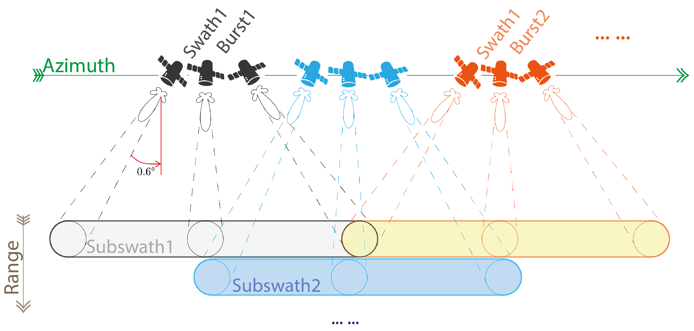
An illustration of TOPS working mode is shown in Figure 1. The squint angle in TOPS introduces the quadratic phase term $\pi K_t{(\eta -{\eta }_c)}^2$ in Equation (14). This term is responsible for the strict coregistration accuracy along azimuth direction. For example, in the presence of a miscoregistration time of $\Delta \eta$ in azimuth direction in the slave image, the interferometric phase error between master and slave would become $2\pi K_t\eta \Delta \eta$ and is a function of azimuth time $\eta$.

For completeness, the IRF as a function of range time $\tau$ is also given [31]:

$$\begin{array}{cc}\hfill s(\tau )& =s_r(\tau )·exp\left\{-j·\frac{4\pi }{\lambda }·R_0\right\}\hfill \\ & ·exp\left\{j·2\pi ·f_0·(cos\beta -1)·(\tau -{\tau }_0)\right\}\hfill \end{array}$$

(15)

$s_r$ is the range envelop of the compressed target and is also typically a $\mathrm{sinc}(·)$ function, $f_0$ is the carrier frequency, $\tau$ is range time, ${\tau }_0$ is the reference range position of the impulse response, and $\beta$ is the squint angle. Due to the presence of squint angle, there is a linear phase term in range direction with slope equal to $f_0(cos\beta -1)$. When $\beta$ is zero this phase ramp disappears; when $\beta$ is significant, the doppler centroid varies in the range direction. In the case of TOPS, the range phase ramp is very small due to the small squint angle in TOPS (±0.6°) and could be neglected [5] in general. Below, we show that a miscoregistration in range direction due to the squint angle $\beta$ together with a strong topology will add a negligible interferometric phase bias. In most cases, the IRF in range direction for TOPS could be treated as the same as the stripmap case.

3.2. Enhanced Spectral Diversity

3.2.1. Introduction to Enhanced Spectral Diversity

Suppose there is a target on the ground with a slight miscoregistration of azimuth time $\Delta \eta$ in the slave image. From Equation (14), the interferogram will be $exp\left\{j{\varphi }_{\mathrm{interf}}\right\}exp\{j2\pi K_t\eta \Delta \eta \}$ where ${\varphi }_{\mathrm{interf}}=4\pi /\lambda ·(R_0,\mathrm{master}-R_0,\mathrm{slave})$. Now, there are two unknown variables, ${\varphi }_{\mathrm{interf}}$ and $\Delta \eta$, but only one observation at time $\eta$. The equation is underdetermined and $\Delta \eta$ cannot be solved.

If there is another observation at time ${\eta }^{\prime }$, then we will have two observations at time $\eta$ and ${\eta }^{\prime }$. With two observations and two unknowns, the system is determined and there is a unique solution to the miscoregistration time $\Delta \eta$. If we write:

$$\begin{array}{cc}\hfill \mathrm{ifg}& =exp\left\{j{\varphi }_{\mathrm{interf}}\right\}exp\{j2\pi K_t\eta \Delta \eta \}\hfill \end{array}$$

(16)

$$\begin{array}{cc}\hfill {\mathrm{ifg}}^{\prime }& =exp\left\{j{\varphi }_{\mathrm{interf}}\right\}exp\{j2\pi K_t{\eta }^{\prime }\Delta \eta \}\hfill \end{array}$$

(17)

Then, the cross-interferogram ([32] uses this term. Meanwhile, some studies call this differential interferogram [3]) is:

$$\begin{array}{c}\hfill \mathrm{ifg}\ast {\mathrm{ifg}}^{\prime }\ast =exp\{j2\pi K_t(\eta -{\eta }^{\prime })\Delta \eta \}\end{array}$$

(18)

As shown in Figure 1, for the same subswath, there is always a small area that is illuminated in consecutive bursts. This means that the target inside this small area are illuminated twice, at time $\eta$ and ${\eta }^{\prime }$ separately. We could use pixels inside this “common area” to generate the cross-interferogram and derive the miscoregistration time $\Delta \eta$ using Equation (18).

3.2.2. 1/1000 Coregistration Accuracy

The common Doppler Centroid rate $K_t$ of focused TOPS is around 1750 Hz/s. Take $(\eta -{\eta }^{\prime })$ to be 2.75 s, suppose one requires a coregistration accuracy that limits the interferogram bias to 0.05 radians, the maximum allowed miscoregistration time $\Delta \eta$ should be 0.05/(2π × 1750 × 2.75) ≈ µs. Taking azimuth PRF of 486 Hz, the miscoregistration time would convert to 0.0008 pixel and round up to 1/1000 pixel. In conclusion, to achieve a coregistration accuracy of 0.05 radians, a 1/1000 pixel coregistration accuracy in azimuth is required.

3.2.3. Phase Ambiguity of ESD

In the ESD step, if the cross-interferogram phase is $\pi$, it corresponds to approximately 104 µs or 0.05 pixel miscoregistration in azimuth. This means that, to avoid the phase ambiguity, the initial coregistration should achieve at least a 0.05 pixel accuracy. Remember that for the stripmap mode, a convention of 1/8 pixel accuracy is desired [1].

4. Evaluation of the Proposed Approach with Test Sites

In this section, we evaluate the performance of the proposed approach with some test sites under different conditions. The focus is on two points:

• The first one is to evaluate the coregistration accuracy of the cross-correlation method by checking the cross-interferogram phase in the ESD step. If the cross-correlation method accuracy is low, then the cross-interferogram phase is away from zero. If the cross-correlation method accuracy is high then the cross interferogram phase is close to zero.
• The second point is to check the interferogram phase difference between the proposed approach and the established approach, and here we treat the established approach as the “reference result”. The aim is to test the correctness and robustness of the proposed approach and to understand the conditions for when the proposed approach could apply.

4.1. Introduction to Test Sites

For the experiment, three different test sites were used. In sequence, the three examples are representing an ideal testing case, a generic testing case, and a case with large topography:

• The first test site is located at the Atacama Desert in northern Chile. The desert is a plateau and is the driest desert in the world. From the InSAR point of view, the site is very coherent. Even interferograms with very long temporal baselines (for example, a few years) could show very high coherence. The idea is to select an ideal case as the first test;
• The second site is a more generic one. This is a pair of data taken in the early summer (April and May 2018) that covers Purdue University, the U.S.A. The surroundings of Purdue University is mostly farmlands and countrysides. There are a few towns inside the area of interest (AOI) connected by the highway. This dataset has 24 days temporal baseline and 60 m spatial baseline. The majority of ground features is distributed scatterers, where the coherence will decrease exponentially in time. In addition, in the Discussion Section, we will present another case in the California Central Valley that shows a very similar ground feature.
• The third site is Mt Etna in Italy. Mt Etna represents a case with large topography and a relatively large spatial baseline of 123 m (in the sense of S1). The highest point of Mt Etna reaches more than 3000 m whereas the lowest point is close to the sea level. The aim is to test the performance of the proposed approach when there is large height variation in the scene.

Meanwhile, when experimenting with the proposed approach, the default patch size as in Equations (1), (2) and (7) that is used for the cross-correlation is 16 by 16. Then the SCR threshold is selected as 7 dB. The selected patch size and SCR threshold value are more of an empirical value that balances between the robustness of the results and the computational power. In addition, the patches are selected to be as uniformly distributed on the image as possible, so that the estimation of the rotation angle as in Equation (11) will be as accurate as possible.

4.2. The Atacama Desert: A Long Swath with 17 Bursts

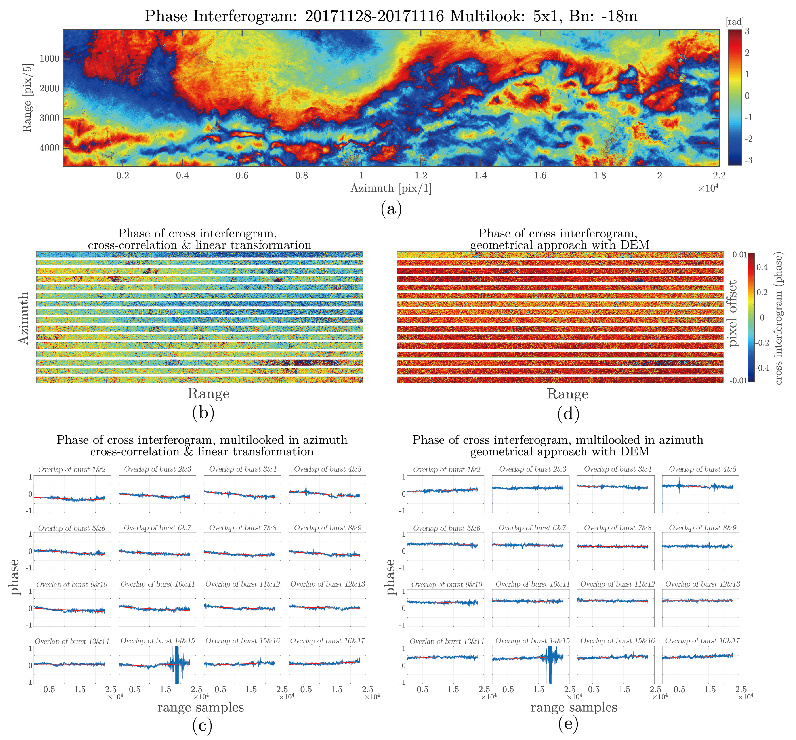
The first example came from Sentinel-1A track 149, subswath 2 on 16 November 2017 and 28 November 2017. The AOI is in the Atacama desert in the northern Chile (dataset used in this example: S1A_IW_SLC__1SDV_20171116T230610_20171116T230637_019296_020B1F_BC1A, S1A_IW_SLC__1SDV_20171116T230635_20171116T230700_019296_020B1F_FC0E, S1A_IW_SLC__1SDV_20171128T230610_20171128T230637_019471_0210A6_4730, S1A_IW_SLC__1SDV_20171128T230635_20171128T230700_019471_0210A6_D735). In the cross-correlation method, 40,295 points with SCR over 7 dB were selected for estimating the rigid transformation coefficients. The cross-interferogram after the cross-correlation method and geometrical method are plotted in Figure 2. Note that only the cross-interferogram at burst overlapping area has a none-zero value. Each burst overlapping area is typically around 100∼120 pixels in azimuth. The cross-interferogram is shown in Figure 2b,d. In addition, to observe the cross-interferogram phase variation in range direction, we multilooked the 100∼120 pixels in azimuth direction for each burst overlapping area and plotted out the cross-interferogram phase as a function of range. The results are shown in Figure 2c,e respectively.

First, using Equation (10), one could calculate that the coregistration accuracy with the cross-correlation method should be approximately 0.001 pixel, or, 0.07 radians in the cross-interferogram. In Figure 2b,c, the average cross-interferogram phase value is approximately 0.01 radians. This shows that the coregistration residual more or less corresponds to the theoretical value.

Second, regardless the initial coregistration method used, the cross-interferogram phases for different bursts overlapping areas are almost the same. This means that even for a very long track (the AOI spans approximately 300 km in azimuth) there is only mainly a mutual shift between the master and slave image after the initial coregistration. In fact, it has been shown that the cross-interferogram phase is consistent in azimuth for even much longer datasets [10,33]. However, the cross-interferogram phases in different bursts show a very small discrepancy in the magnitude of 0.1 radians. A number of reasons could contribute to such small discrepancy in different bursts. The typical contributing factors could be orbit inaccuracies, timing errors, or geophysical effects [5,34,35].

Finally, the cross-interferogram phase in the geometrical method does not vary much in range (Figure 2e). This has been reported by others [3,33,35] as well. On the other side, the cross-interferogram phase after rigid transformation is sometimes showing a linear trend in the range direction with a noticeable slope (Figure 2c). The reason is a small rotation angle estimation error. More details are presented in the Discussion Section.

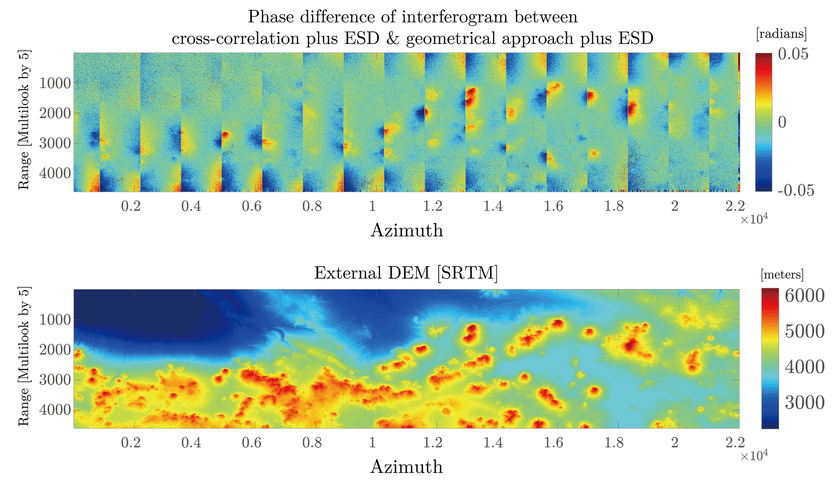
In Figure 3 the phase difference between the two interferograms from the proposed approach (cross-correlation followed by ESD) and the established approach (geometrical followed by ESD) is plotted. Overall, the phase difference is within 0.05 radians in most part of AOI, meaning that the difference between two approaches is within the error margin at most parts. Still, it could be seen that the phase difference at some places exceeds 0.05 radians. The places with large phase difference have the following common characteristics:

• They all have very large height values (comparing with the mean height of the AOI);
• They are all located at or near the the edges of bursts.

This non-negligible phase difference should mainly come from a miscoregistration in the azimuth direction due to the presence of the crossing angle and the fact that the topography is not considered during cross-correlation method [14]. Another similar case will be presented in the following subsection.

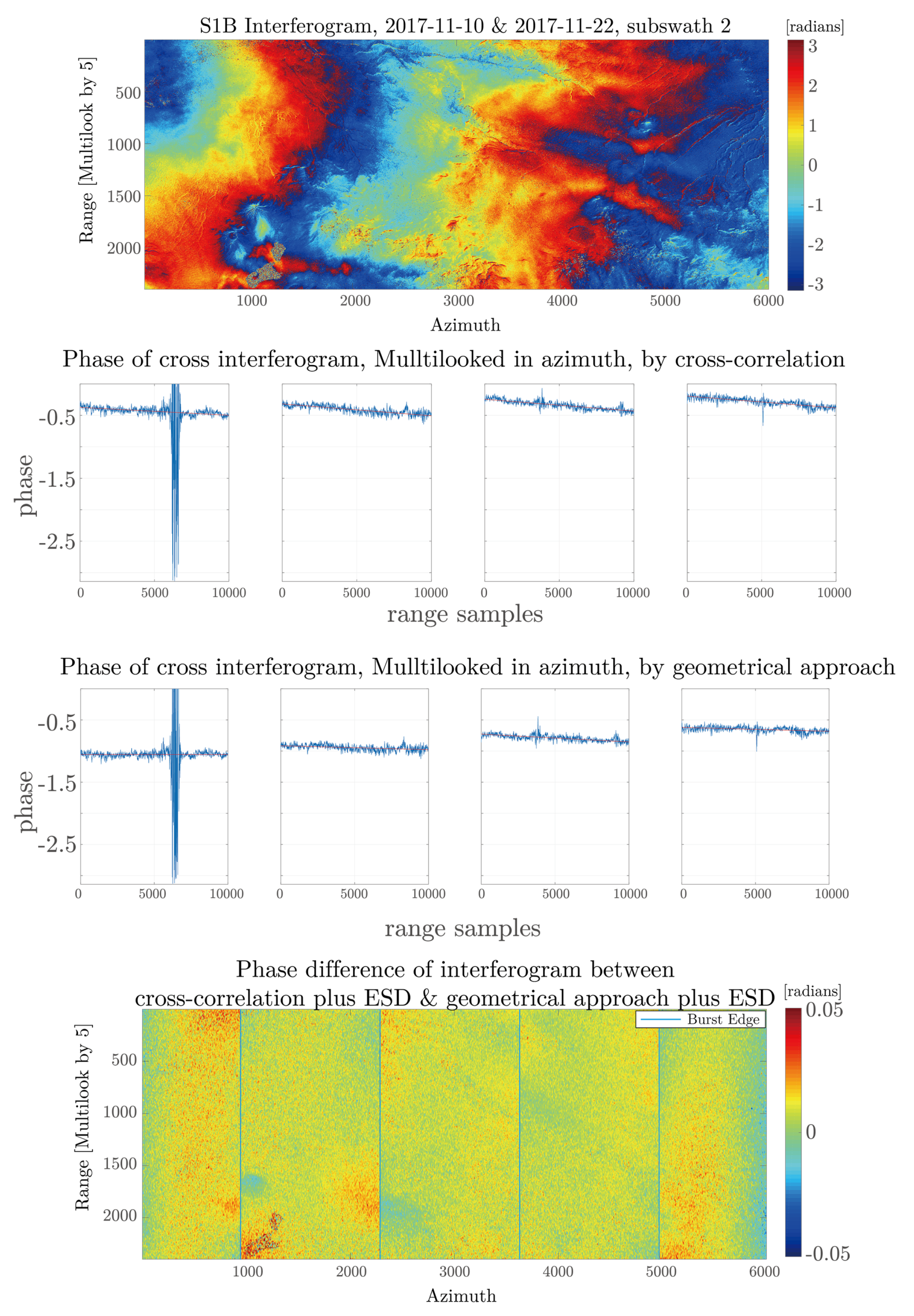
4.3. The Atacama Desert: A Short Swath With 4 Bursts

Examples of a smaller area (range 10,000 by azimuth 6000) is shown in Figure 4. The two SLCs come from Sentinel-1B track 149, subswath 2 on 10 November 2017 and 22 November 2017 in the same area (dataset used in this example: S1B_IW_SLC__1SDV_20171110T230533_20171110T230600_008225_00E8C3_1BA6, S1B_IW_SLC__1SDV_20171122T230533_20171122T230559_008400_00EE11_75CF). A total of 7795 patches with SCR greater than 7 dB are selected for the cross-correlation method. The theoretical coregistration accuracy should be on the scale of 0.15 radians on cross-interferogram. In Figure 4, the phase read from cross-interferogram is slightly larger than this theoretical value, but they are still more or less at the same level of magnitude. For showing the correctness of the proposed approach, one could see that the phase difference in interferograms is well limited to within −0.02 to 0.02 radians.

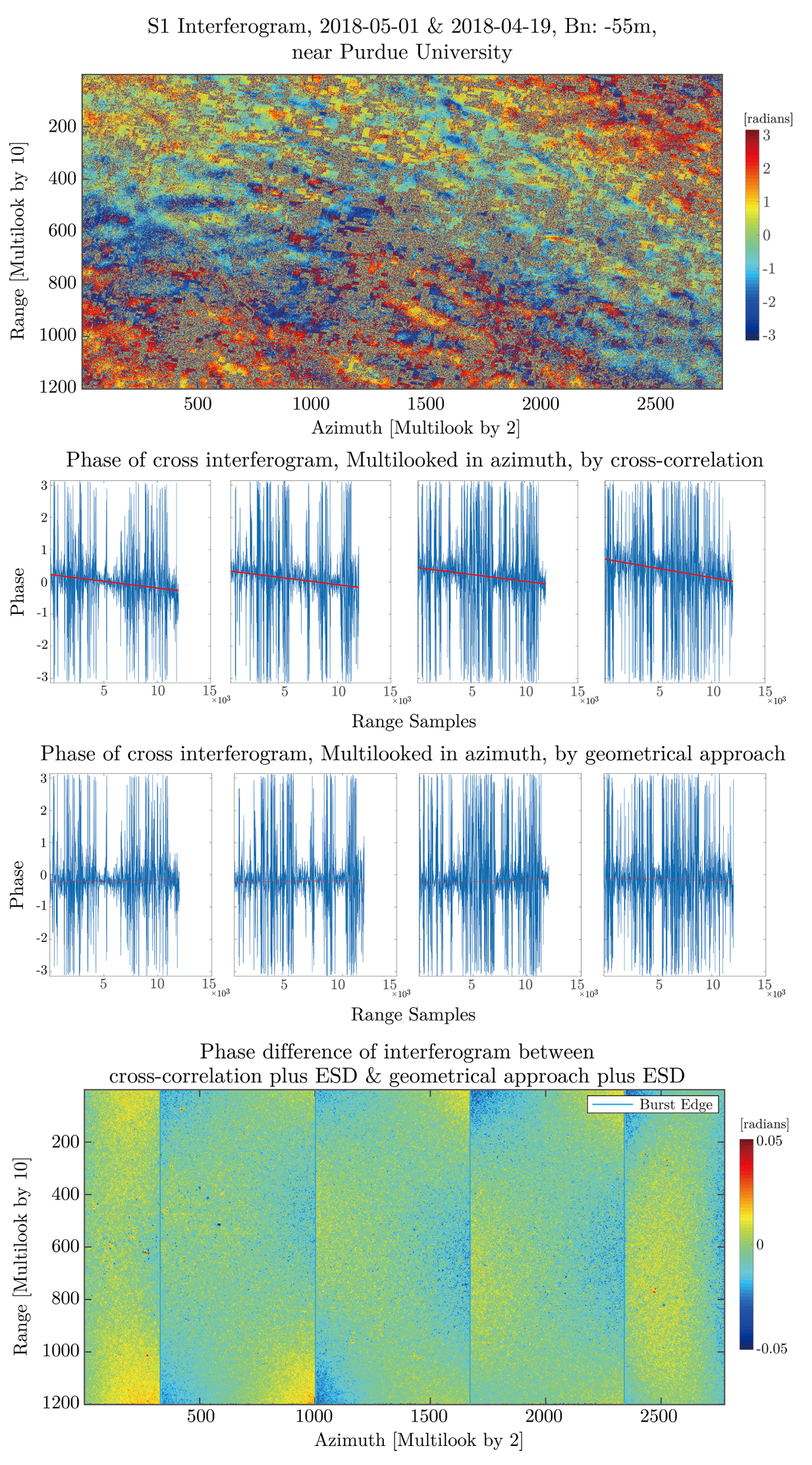
4.4. Purdue University: An Example with 24 Days Temporal Baseline in April

This example includes two S1A data in April and May with 24 days temporal baseline and 55 m spatial baseline (dataset used in this example: S1A_IW_SLC__1SDV_20180419T234016_20180419T234044_021543_0251FA_381A, S1A_IW_SLC__1SDV_20180501T234017_20180501T234045_021718_02577C_001E). Subswath 2 covers the entire Purdue University, and the area is typical farmland with scattered small towns (such as the university campus). From the interferogram in Figure 5, one can see the “blocks” that represent different types of crops. The noisy “blocks” should indicate the fast growth of some types of crops in April; while the coherent “blocks” could indicate no changes over the 24 days period.

The cropped area has 12,000 pixels in range and 5550 pixels in azimuth. The interferogram is multilooked by 10 × 2 with no filters applied. 1229 patches with SCR higher than 7 dB are selected for estimating the rigid transformation matrix. In theory (Equation (8) and (10)), this would correspond to around 0.05 pixel coregistration accuracy, or around 0.37 radians in the cross-interferogram. The average of the cross-interferogram phase read from the four burst overlaps is 0.42, which is pretty close to the theory.

Comparing with the previous case of the Atacama desert, the cross interferogram of this example looks less coherent due to the temporal decorrelation of distributed scatterers. However, the final interferogram phase between the proposed approach and the established approach shows a very small difference that is limited to within the 0.05 radians error margin. This example shows that the proposed approach could also work well in a more generic case.

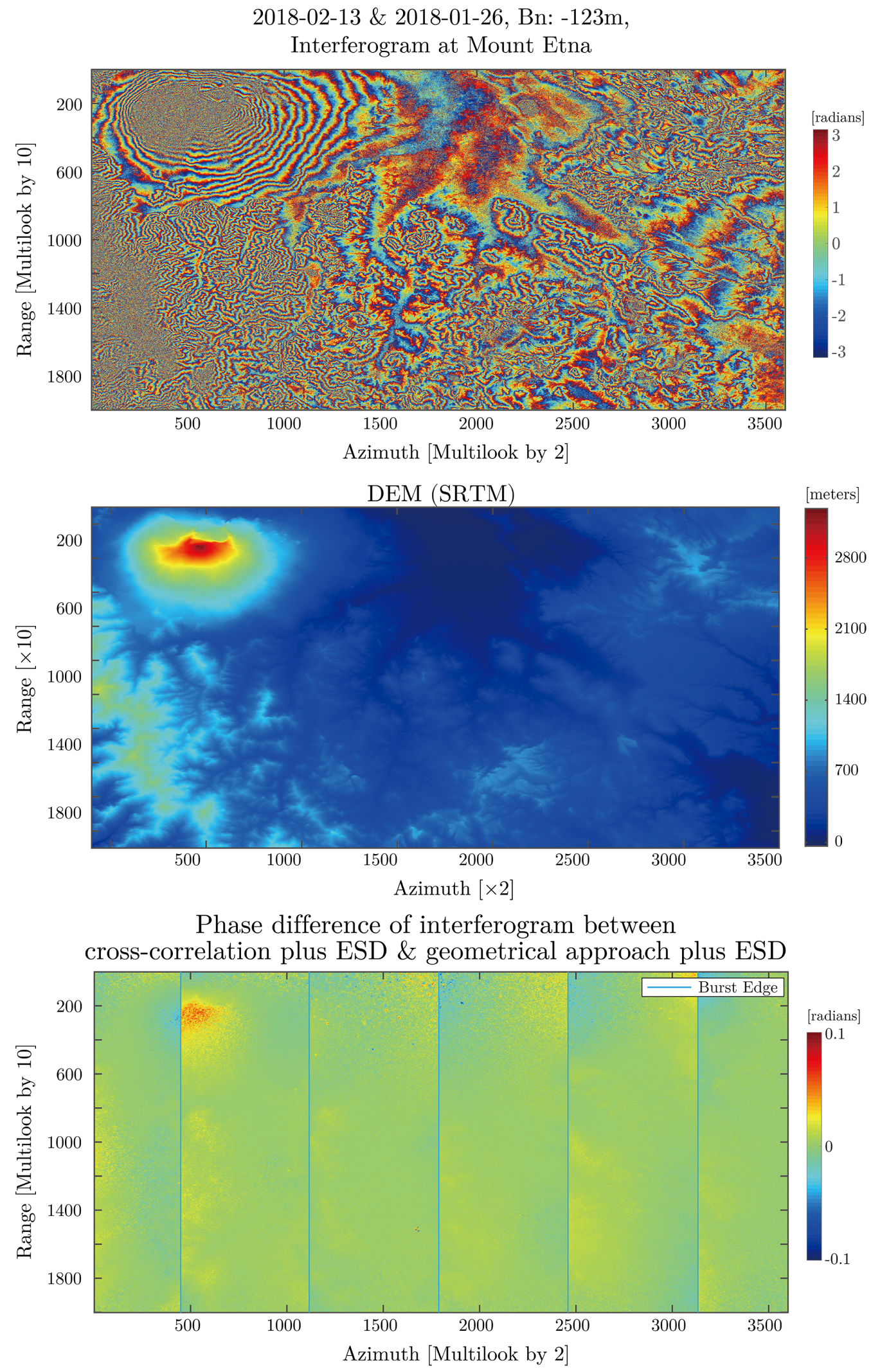
4.5. Mt Etna: An Example With Large Topography and 123 m Spatial Baseline

Mt Etna is an active volcano on the island of Sicily, Italy, and its height is 3329 m. The purpose of this testing site is to understand the effect of large topography to the proposed approach. To make this case more general, a relatively large spatial baseline (for Sentinel-1 case) of 123 m is selected. The temporal baseline is 18 days (dataset used in this example: S1A_IW_SLC__1SDV_20180126T050434_20180126T050501_020321_022B4C_48A0, S1B_IW_SLC__1SDV_20180213T050354_20180213T050428_009600_0114CD_9865).

The result is shown in Figure 7. The cropped area has 19,000 pixels in range and 7200 pixels in azimuth. The interferogram is multilooked by 10 × 2 with no filters applied. To highlight the location of the volcano, the topography phase is not removed from the interferogram. In the rigid transformation, 10054 patches with SCR higher than 7 dB are selected for estimating the rigid transformation matrix.

The interferogram phase difference between the proposed approach and the established approach shows a very similar pattern as in the case of the Atacama desert:

• (To use the established approach as the reference, then). The interferogram phase error correlates with the topography. The phase error is the largest at the top of the mountain.
• The interferogram phase correlates with the azimuth position inside the burst. The phase error is the largest at burst edges and tends toward zero at the center of the burst.

In this Mt Etna case, the phase discrepancy at the top of the mountain could reach 0.1 radians or more. Similar to the case in Section 4.2, this phase residual should mainly come from the miscoregistration in the azimuth direction due to the orbital crossing angle and the fact the cross-correlation method fails to consider the topography during coregistration. This effect was well analyzed in [14]. The conclusion is that for cases with very large height variation in the AOI, the proposed approach will introduce a non-negligible phase bias at or near burst edges by failing to consider the DEM during coregistration.

5. Further Discussion

5.1. The Rotation of Slave Image

In all the examples that are shown in the previous section, when using the proposed approach, it can be seen that linear slopes appears in the range direction on the cross-interferogram phase. The linear slope is caused by the residual rotation angle of slave image during the rigid transformation estimation process.

For the purpose of doing interferometry, it is desired to have perfect parallel repeat pass satellite orbits. However, due to the eccentricity of ellipsoid earth, one could never get a perfect parallel between the repeat pass. There will be a very small crossing angle [14]. The crossing angle, albeit small, could introduce some error to the TOPS interferogram. There are mainly three effects for the crossing angle: (1) It will introduce a small amount of burst mis-synchronization and spectrum decorrelation to TOPS [14]. The mis-synchronization could be corrected by the ESD and the decorrelation could be corrected by applying an azimuth common-bandwidth filter (or, since the burst mis-synchronization is usually very small for TOPS, mostly under 5% [34,36], one could just ignore the minor coherence loss there); (2) The small crossing-angle post an accuracy requirement to the availability of DEM when performing geometrical coregistration. Though the requirement is quite low, an accuracy of around 300 m in DEM is still needed to keep the interferometric phase error under 1.5° [14]. (3) The last one is for the proposed approach. Since there will be a small rotation between master and slave due to the small crossing angle, the rigid transformation will estimate this rotation angle. The residual between the true rotation angle and the estimated rotation angle will introduce this linear slope in the cross-interferogram.

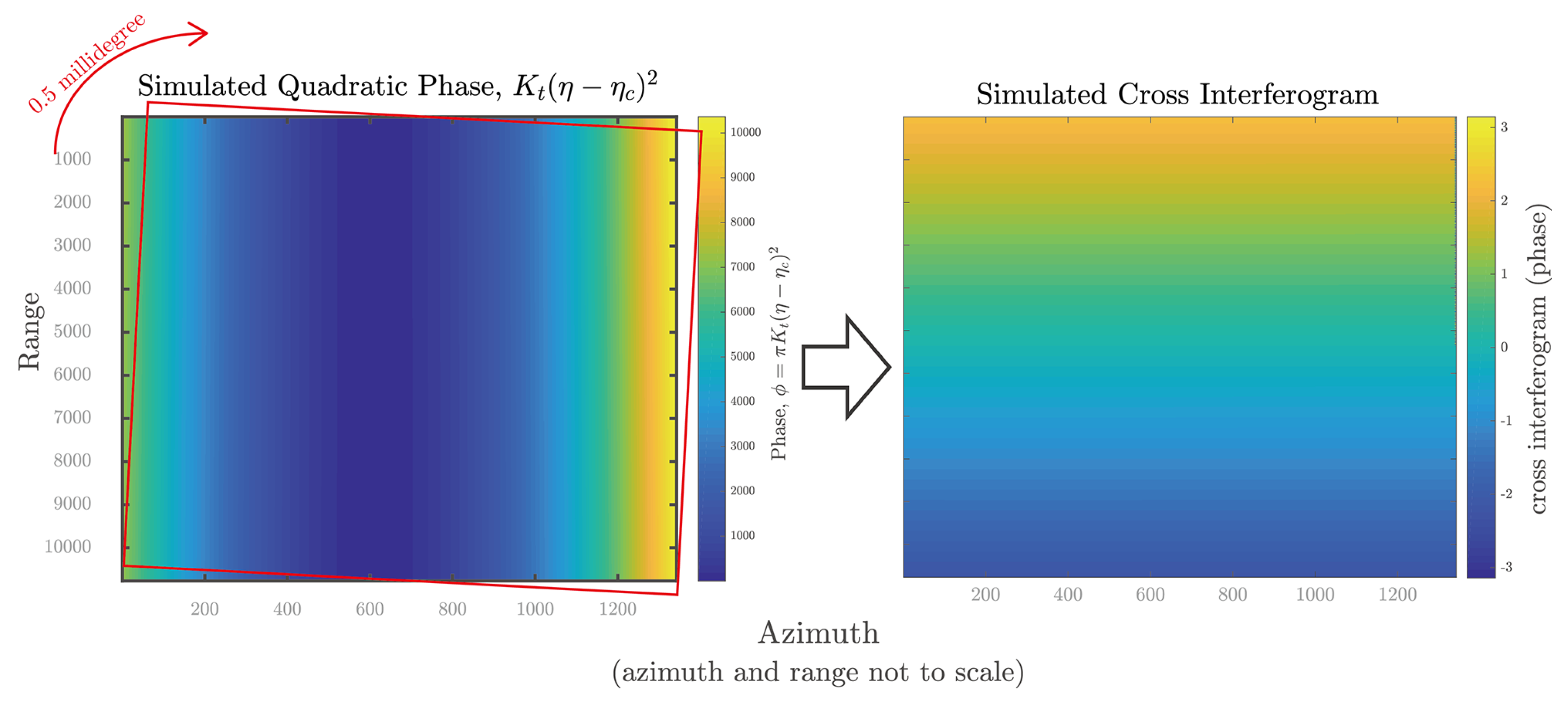
We start by simulating a small rotation between master and slave image using the real parameters from TOPS. The steps are: (1) read the quadratic phase parameters from a real sample dataset, specifically $K_t$ and ${(\eta -{\eta }_c)}^2$ [29]; (2) rotate the quadratic phase by a small angle in the counterclockwise direction around its center point; and (3) simulate the two looks from two difference squint angles and generate the cross-interferogram.

The simulation result is shown in Figure 6. A rotation angle error of 0.5 millidegree corresponds to a linear slope in range of approximately 4.1 × 10⁻⁴ radians/sample on the cross-interferogram. In our example, the phase changes 4.4 radians in range over the 10770 samples. To correct the rotation error, when performing the ESD one should estimate the range slope and compensate for the rotation angle error. Since the phase could be wrapped, the estimation of the slope could be done with the Fourier transform. Estimating the slope of cross interferogram phase is equivalent to finding the peak of shift after Fourier transform:

$$\begin{array}{c}\hfill x(\tau )exp\left\{-j2\pi f_{\mathrm{rot}}\tau \right\}\stackrel{\mathcal{F}}{\to }X(f-f_{\mathrm{rot}})\\ \hfill {\widehat{f}}_{\mathrm{rot}}=argmaxX(f-f_{\mathrm{rot}})\end{array}$$

(19)

where $f_{\mathrm{rot}}$ is the desired slope in range for the cross interferogram. The range slope in the cross-interferogram only depends on the residual rotation angle and does not depend on the mutual shift between master and slave. The bigger the rotation angle, the steeper the slope.

According to [14], at the initial stage of S1 mission, the crossing angle reaches one millidegree in the worst case. Later, ESA tightened the cross angle to less than 0.25 millidegree. However, as shown in the simulation, a 0.25 millidegree rotation error could indicate almost a full $2\pi$ phase variation along a full burst (usually around 24,000 samples in range). Even a very small estimation error in the rotation angle could be clearly observed on the cross interferogram as a slope in range. In conclusion, it is very necessary to estimate and correct this rotation angle estimation error when using the proposed approach.

At last, it can be inferred from the examples that the correctness of the final interferogram product from the proposed approach depends on how well one can estimate the phase and slope from the cross-interferogram in the presence of the noise. When interferogram coherence is low, the cross interferogram will be noisier, and the estimation of coregistration residuals from interferogram will be less accurate. This also means that, for a more robust ESD, it is desired to choose image pairs of shorter temporal baseline and hence less temporal decorrelation effect.

5.2. DEM Related Distortions in TOPS Interferogram

Finally, we discuss the impact of DEM in TOPS coregistration and interferometry. DEM/topography could influence the TOPS interferometric process in a number of different ways. In this section we discuss a few error sources when DEM is not available and how the absence of DEM would bias the interferogram.

The first impact of DEM is related to the crossing angle. As appears in Equation (12), the accuracy requirement of DEM increase with an increasing crossing angle [12]. Since the crossing angle for S1 is much smaller than the case of ERS or Envisat, the requirement on DEM is not so strict. For example, for a 0.001° crossing angle, one only needs DEM accuracy of around 300 m to fulfill the TOPS coregistration requirement [14]. In general, for flat areas with height deviation smaller than a couple of hundred meters, one could use the earth ellipsoid model instead of SRTM. In our example in Figure 3 and Figure 7 with large topography deviation, it is still important to have the SRTM when using the established approach. More details for TOPS case could be found in [4,14]. The general idea is that an available SRTM as the DEM is good enough for an accurate coregistration in the established approach. The second impact that DEM has is the azimuth positioning error due to a change of effective velocity and squinting angle. In general, since the baseline of S1 is usually very small, the difference between master and slave effective velocity is very small, thus the interferometric phase difference with or without using DEM due to this factor is negligible [37].

5.3. The Break down Point of Cross-Correlation Method

This section explores the breakdown point for correctly performing the proposed approach. From the previous discussion, we know that there should be two factors in general. The first factor is whether there are enough points with high SCR to estimate the rigid transformation matrix and avoiding the phase ambiguity in the ESD. The second factor is whether the cross-interferogram phase is too noisy to obtain a robust estimation of the phase and slope value in ESD.

5.3.1. Are There Enough Points for Rigid Transformation to Avoid ESD Phase Ambiguity?

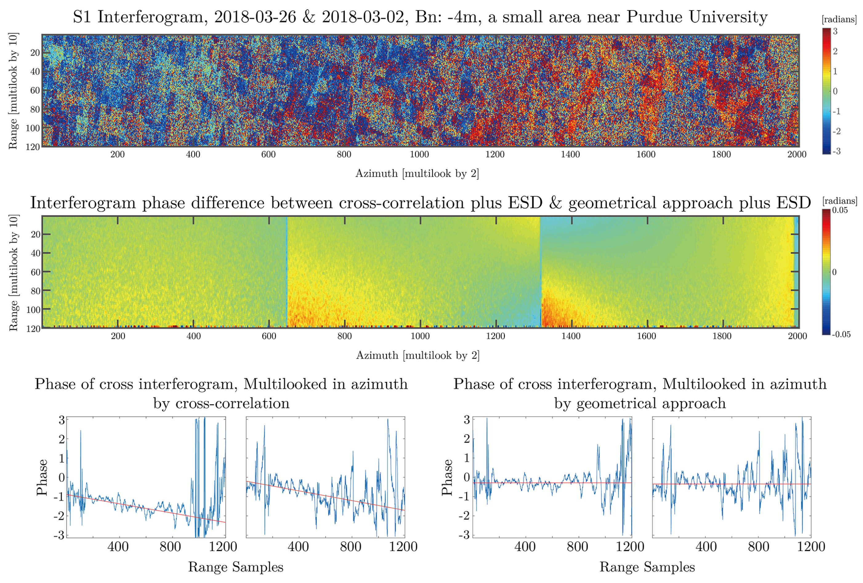
The previous calculation shows that a 0.05 pixel coregistration accuracy is enough for avoiding the ESD phase ambiguity. In theory, this is equivalent to around 10 strong scatterers with SCR over 10 dB. In most cases, this should be a relatively easy goal to reach, even when one’s processing area is small. Then, the ESD step is able to compensate for the coregistration residuals (assuming that the estimation of ESD phase and slope is correct).

Here, one interferogram near Purdue University with 24 days temporal baseline is given (dataset used in this example: S1A_IW_SLC__1SDV_20180302T234015_20180302T234043_020843_023BEE_CDC1,

S1A_IW_SLC__1SDV_20180326T234016_20180326T234044_021193_02470B_BE68). The AOI has 1200 range samples and 4000 azimuth lines, making it a relatively small area. Again, the majority of AOI consists of distributed scatterers. In the cross-correlation process, 120 points with SCR over 7 dB were selected for estimating and performing the rigid transformation. This corresponds to 0.02 pixel coregistration accuracy, or 1.2 radians in cross-interferogram phase. In Figure 8, the average phase from the cross-interferogram is more or less this value; however the rotation angle estimation error in this case is larger. However, the example shows that around 100 points is enough for the cross-correlation method to avoid the phase ambiguity in ESD. The difference in interferogram between the proposed approach and the established approach is mostly limited to within 0.05 radians. A few spots still show phase difference approaching 0.05 radians. This discrepancy should mainly come from the estimation error of the ESD phase and slope, which will be discussed in the next section.

5.3.2. Cross-Correlation Method with Long Temporal Baseline

As discussed in previous sections, for the established approach, the coregistration residual after the geometric approach is mainly a constant value, so that one could conveniently estimate one value for one burst overlapping area. However, in the cross-correlation method, there is the rotation angle estimation error, which will be reflected as a linear slope in the range direction on the cross interferogram. The slope needs to be estimated and removed. If the slope is wrongly estimated, the error will propagate to the interferogram.

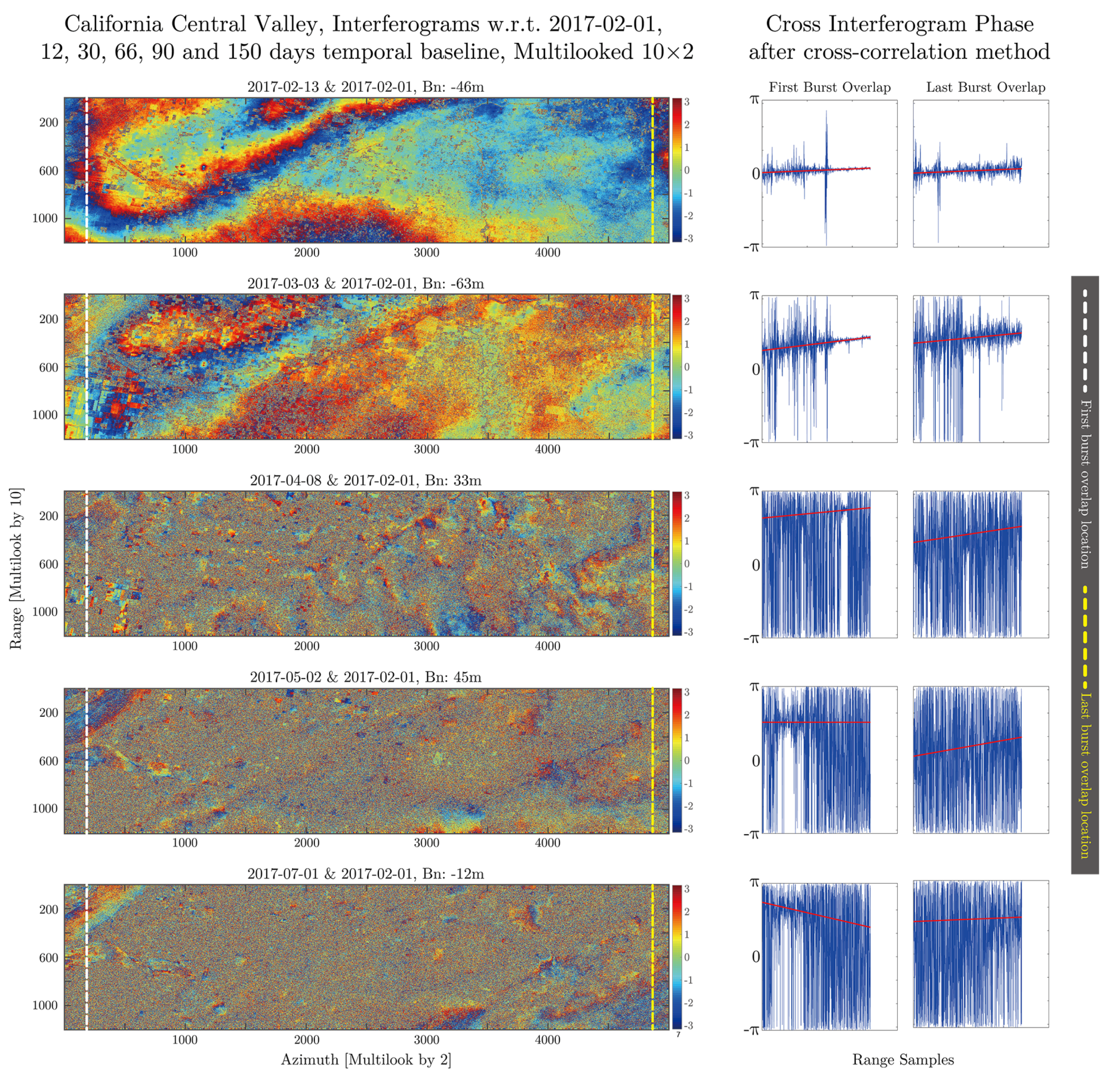
The accuracy of estimation depends on the SNR of the cross-interferogram phase, or equivalently, the coherence. It is already well known that the coherence decreases as spatial and temporal baseline increase. For Sentinel-1, the spatial baseline is well controlled to a small orbital tube, so that the spatial decorrelation is not the key factor here. In this experiment, we use the proposed approach for image pairs with from 12 days to 150 days temporal baseline. The test site is the California Central Valley. The California Central Valley is a flat valley in the center of California, and the majority of the valley is vegetated. The situation is very similar to the previous test case of Purdue University. For the experiment, the image on 1 February 2018 was set as the master and was paired up with images from 12 days to 150 days apart. Each image has 12000 range pixels and 10000 azimuth lines. Five interferograms with 12, 30, 66, 90 and 150 days temporal baseline are shown in Figure 9. The interferograms were multilooked by 10 × 2.

The interferogram decorrelates exponentially with temporal baseline. In this example, the 12-days-baseline and 30-days-baseline still shows a “clean” cross-interferogram, where the slope could be well estimated with a higher significance level. Then as the temporal baseline increase, the interferogram becomes noisier, and the estimation of ESD phase & slope will have much lower significance level. When the cross-interferogram is incoherent and the estimation is not precise, then the coregistration error will be carried into the interferogram as the phase error.

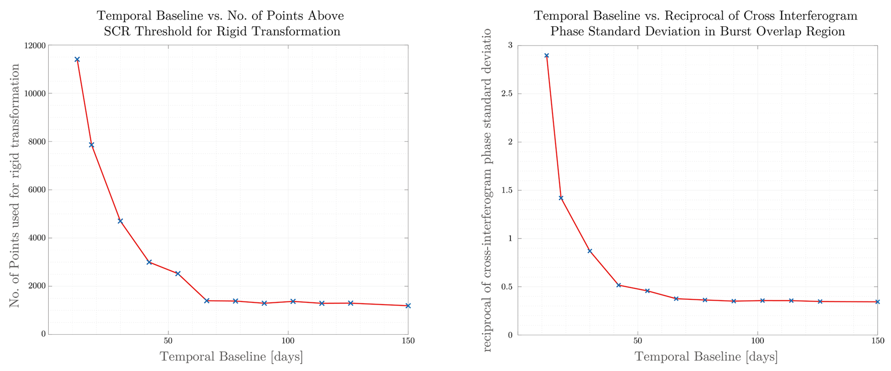
Figure 10 shows the cross-interferogram phase standard deviation as a function of temporal baseline. For each pair of images, the phase standard deviation is the average for all burst overlaps in the cross-interferogram. It could be observed that the reciprocal of phase standard deviation decays exponentially in time. At around 60 days, the value reaches approximately 0.35 and stays more or less the same afterward. Consider a scene with complete circular Gaussian noise, then the phase should be uniformly distributed and the phase standard deviation is ${\pi }^2/3$, roughly around 3.3, making the reciprocal value around 0.3. This means that at around 60 days the cross-interferogram becomes almost totally noisy and the estimated phase & slope might not be reliable.

On the other side, although the number of points with SCR higher than 7 dB also decreases exponentially in time, after 60 days, the value becomes quite stable at around 1000. As discussed in the previous section, this number is still enough for avoiding the ESD phase ambiguity. Thus, the key to a successful coregistration is to select pairs with short temporal baseline and coherent interferometric phase. This test dataset shows that it is possible to get a good estimation of phase and slope for temporal baseline shorter than 50 days. After that, the cross-interferogram might be too noisy, and the estimation will have a lower level of significance, possibly giving a non-negligible error to the interferogram.

It is worth noting that, for a time series analysis, with the aforementioned discussion, it is thus not recommended to use a single-master approach to perform the proposed approach. For retrieving coherent image pairs, one can either use the MST graph or a redundant graph approach [33,38]. The other improvement that could be done is to estimate the ESD phase and slope not with the full burst overlapping area, but only with strong and coherent scatterers (that are not affected by noise).

6. Conclusions

In this work, we studied the coregistration accuracy using the cross-correlation and rigid-transformation method (referred to as “cross-correlation method” throughout the article) and analyzed the feasibility, correctness, and robustness of coregistering Sentinel-1 TOPS images using the cross-correlation method followed by the enhanced spectral diversity (referred to as “proposed approach”). We used the idea of Cramér-Rao lower bound to study the accuracy of the two key steps in the cross-correlation method. Based on the analysis of CRLB, the coregistration accuracy mainly depends on the number and signal clutter ratio of points/patches that are available for the rigid transformation. For increasing the coregistration accuracy, it is desired to have more points with higher SCR.

In the proposed approach, the rigid transformation step estimates a rotation angle for the slave image. An estimation error of the rotation angle, albeit small, introduces a modulation in range to the cross interferogram and is reflected as a linear slope on the cross interferogram phase in range. For successfully performing the proposed approach, a key step is to estimate well the starting phase and the slope, thus to correct the rotation angle error.

To verify the correctness of the proposed approach, we compared the interferogram from the proposed approach with the established approach (geometrical plus ESD). The experiments show that the most important factor for success is the coherence of cross interferogram. For example, when the area is less coherent, the estimation of slope in ESD might not be precise, and the interferogram might be erroneous. The most likely contributing factor to a low coherence is the temporal decorrelation. However, in the two general cases (Purdue University and the California Central Valley), for a site that is dominated by vegetated land and has 24 or 30 days temporal baseline, the proposed approach could work well. Work well means that the interferogram difference between the proposed approach and the established approach is mostly within the 0.05 radians error margin.

To avoid the phase ambiguity in the ESD step, the experiments show that 100 points or more is already good enough, which is relatively easy to achieve. However, with smaller areas or less coherent areas, the question again becomes whether the estimation in the ESD step could be successfully performed with a high confidence level.

Finally, for areas with large topography variation, due to the presence of the orbital crossing angle, and the fact that the proposed approach failed to consider the topography during coregistration, there will be an azimuth miscoregistration and this will introduce a non-negligible phase error. For Mt Etna case with 123 m normal baseline and 3000 m height variation, this topographic miscoregistration will introduce at most 0.1 radians of interferometric error.

References

- Just, D.; Bamler, R. Phase statistics of interferograms with applications to synthetic aperture radar. Appl. Opt. 1994, 33, 4361–4368. [Google Scholar] [CrossRef] [PubMed]
- De Zan, F.; Monti Guarnieri, A. TOPSAR: Terrain Observation by Progressive Scans. IEEE Trans. Geosci. Remote Sens. 2006, 44, 2352–2360. [Google Scholar] [CrossRef]
- Prats-Iraola, P.; Scheiber, R.; Marotti, L.; Wollstadt, S.; Reigber, A. TOPS interferometry with TerraSAR-X. IEEE Trans. Geosci. Remote Sens. 2012, 50, 3179–3188. [Google Scholar] [CrossRef] [Green Version]
- Scheiber, R.; Jäger, M.; Prats-Iraola, P.; De Zan, F.; Geudtner, D. Speckle tracking and interferometric processing of TerraSAR-X TOPS data for mapping nonstationary scenarios. IEEE J. STARS 2015, 8, 1709–1720. [Google Scholar] [CrossRef]
- De Zan, F. Accuracy of Incoherent Speckle Tracking for Circular Gaussian Signals. IEEE Geosci. Remote Sens. Lett. 2014, 11, 264–267. [Google Scholar] [CrossRef] [Green Version]
- Wright, T.J.; Biggs, J.; Crippa, P.; Ebmeier, S.K.; Elliott, J.; Gonzalez, P.; Hooper, A.; Larsen, Y.; Li, Z.; Marinkovic, P.; et al. Towards Routine Monitoring of Tectonic and Volcanic Deformation with Sentinel-1. In Proceedings of the ESA FRINGE Workshop, Frascati, Italy, 23–27 March 2015. [Google Scholar]
- Geudtner, D.; Torres, R.; Snoeij, P.; Davidson, M. Sentinel-1 System Overview. In Proceedings of the ESA FRINGE Workshop, Frascati, Italy, 19–23 September 2011; pp. 1–6. [Google Scholar]
- Miranda, N.; Meadows, P.; Hajduch, G.; Pilgrim, A.; Piantanida, R.; Giudici, D.; Small, D.; Schubert, A.; Husson, R.; Vincent, P.; et al. The Sentinel-1A instrument and operational product performance status. In Proceedings of the 2015 IEEE International Geoscience and Remote Sensing Symposium (IGARSS), Milan, Italy, 26–31 July 2015; pp. 2824–2827. [Google Scholar]
- Potin, P.; Rosich, B.; Grimont, P.; Miranda, N.; Shurmer, I.; O’Connell, A.; Torres, R.; Krassenburg, M. Sentinel-1 mission status. In Proceedings of the 11th European Conference on Synthetic Aperture Radar, Hamburg, Germany, 6–9 June 2016; pp. 1–6. [Google Scholar]
- Yagüe-Martínez, N.; Prats-Iraola, P.; González, F.R.; Brcic, R.; Shau, R.; Geudtner, D.; Eineder, M.; Bamler, R. Interferometric Processing of Sentinel-1 TOPS Data. IEEE Trans. Geosci. Remote Sens. 2016, 54, 2220–2234. [Google Scholar] [CrossRef]
- Ferretti, A.; Monti Guarnieri, A.; Prati, C.; Rocca, F. InSAR processing: A practical approach. In InSAR Principles: Guidelines for SAR Interferometry Processing and Interpretation; ESA Publications: Paris, France, 2007. [Google Scholar]
- Sansosti, E.; Berardino, P.; Manunta, M.; Serafino, F.; Fornaro, G. Geometrical SAR image registration. IEEE Trans. Geosci. Remote Sens. 2006, 44, 2861–2870. [Google Scholar] [CrossRef]
- Scheiber, R.; Moreira, A. Coregistration of interferometric SAR images using spectral diversity. IEEE Trans. Geosci. Remote Sens. 2000, 38, 2179–2191. [Google Scholar] [CrossRef]
- Prats-Iraola, P.; Rodriguez-Cassola, M.; Lopez-Dekker, P.; Scheiber, R.; De Zan, F.; Barat, I.; Geudtner, D. Considerations of the Orbital Tube for Interferometric Applications. In Proceedings of the ESA FRINGE Workshop, Frascati, Italy, 23–27 March 2015. [Google Scholar]
- Mancon, S.; Monti Guarnieri, A.; Tebaldini, S. Sentinel-1 precise orbit calibration and validation. In Proceedings of the ESA FRINGE Workshop, Frascati, Italy, 23–27 March 2015. [Google Scholar]
- Knapp, C.; Carter, G. The generalized correlation method for estimation of time delay. IEEE Trans. Acoust. Speech Signal Process. 1976, 24, 320–327. [Google Scholar] [CrossRef]
- Stein, S. Algorithms for ambiguity function processing. IEEE Trans. Acoust. Speech Signal Process. 1981, 29, 588–599. [Google Scholar] [CrossRef]
- Bamler, R.; Eineder, M. Accuracy of Differential Shift Estimation by Correlation and Split-Bandwidth Interferometry for Wideband and Delta-k SAR Systems. IEEE Geosci. Remote Sens. Lett. 2005, 2, 151–155. [Google Scholar] [CrossRef]
- Bamler, R. Interferometric stereo radargrammetry: Absolute height determination from ERS-ENVISAT interferograms. In Proceedings of the 2000 IEEE International Geoscience and Remote Sensing Symposium (IGARSS), Honolulu, HI, USA, 24–28 July 2000; Volume 2, pp. 742–745. [Google Scholar]
- Hanssen, R.F. Stochastic model for radar interferometry. In Radar Interferometry: Data Interpretation and Error Analysis; Springer: Berlin, Germany, 2001; Volume 2. [Google Scholar]
- Carter, G.C. Coherence and time delay estimation. Proc. IEEE 1987, 75, 236–255. [Google Scholar] [CrossRef]
- Zebker, H.A.; Villasenor, J. Decorrelation in interferometric radar echoes. IEEE Trans. Geosci. Remote Sens. 1992, 30, 950–959. [Google Scholar] [CrossRef] [Green Version]
- Patri, C.; Rocca, F. Range Resolution Enhancement with Multiple Sar Surveys Combination. In Proceedings of the IGARSS ’92 International Geoscience and Remote Sensing Symposium, Houston, TX, USA, 26–29 May 1992; Volume 2, pp. 1576–1578. [Google Scholar]
- Serafino, F. SAR image coregistration based on isolated point scatterers. IEEE Geosci. Remote Sens. Lett. 2006, 3, 354–358. [Google Scholar] [CrossRef]
- Yetik, I.S.; Nehorai, A. Performance bounds on image registration. IEEE Trans. Signal Process. 2006, 54, 1737–1749. [Google Scholar] [CrossRef]
- Li, J.; Huang, P. A comment on “performance bounds on image registration”. IEEE Trans. Signal Process. 2009, 57, 2432–2433. [Google Scholar]
- Mancon, S.; Guarnieri, A.M.; Giudici, D.; Tebaldini, S. On the phase calibration by multisquint analysis in TOPSAR and stripmap interferometry. IEEE Trans. Geosci. Remote Sens. 2017, 55, 134–147. [Google Scholar] [CrossRef]
- Biggs, J.; Wright, T.; Lu, Z.; Parsons, B. Multi-interferogram method for measuring interseismic deformation: Denali Fault, Alaska. Geophys. J. Int. 2007, 170, 1165–1179. [Google Scholar] [CrossRef] [Green Version]
- Miranda, N. Definition of the TOPS SLC Deramping Function for Products Generated by the S-1 IPF; Techreport COPE-GSEG-EOPG-TN-14-0025; ESA Publications: Paris, France, 2015. [Google Scholar]
- Piantanida, R.; Hajduch, G.; Poullaouec, J. Sentinel-1 Level 1 Detailed Algorithm Definition; Techreport SEN-TN-52-7445; ESA Publications: Paris, France, 2016. [Google Scholar]
- Bara, M.; Scheiber, R.; Broquetas, A.; Moreira, A. Interferometric SAR signal analysis in the presence of squint. IEEE Trans. Geosci. Remote Sens. 2000, 38, 2164–2178. [Google Scholar] [CrossRef] [Green Version]
- Grandin, R. Interferometric processing of SLC Sentinel-1 TOPS data. In Proceedings of the ESA FRINGE Workshop, Frascati, Italy, 23–27 March 2015. [Google Scholar]
- Fattahi, H.; Agram, P.; Simons, M. A Network-Based Enhanced Spectral Diversity Approach for TOPS Time-Series Analysis. IEEE Trans. Geosci. Remote Sens. 2017, 55, 777–786. [Google Scholar] [CrossRef] [Green Version]
- Yagüe-Martínez, N.; González, F.R.; Brcic, R.; Shau, R. Interferometric Evaluation of Sentinel-1A TOPS data. In Proceedings of the ESA FRINGE Workshop, Frascati, Italy, 23–27 March 2015. [Google Scholar]
- Larsen, Y.; Marinkovic, P. Sentinel-1 TOPS data coregistration operational and practical considerations. In Proceedings of the ESA FRINGE Workshop, Frascati, Italy, 23–27 March 2015. [Google Scholar]
- Schwerdt, M.; Schmidt, K.; Tous Ramon, N.; Klenk, P.; Yague-Martinez, N.; Prats-Iraola, P.; Zink, M.; Geudtner, D. Independent system calibration of Sentinel-1B. Remote Sens. 2017, 9, 511. [Google Scholar] [CrossRef]
- Rodriguez-Cassola, M.; Prats-Iraola, P.; De Zan, F.; Scheiber, R.; Reigber, A.; Geudtner, D.; Moreira, A. Doppler-related distortions in TOPS SAR images. IEEE Trans. Geosci. Remote Sens. 2015, 53, 25–35. [Google Scholar] [CrossRef]
- Yagüe-Martínez, N.; De Zan, F.; Prats-Iraola, P. Coregistration of Interferometric Stacks of Sentinel-1 TOPS Data. IEEE Geosci. Remote Sens. Lett. 2017, 14, 1002–1006. [Google Scholar] [CrossRef]
Figure 1.
An illustration of TOPS working mode.
Figure 2.
Interferogram of two S1A images on 16 November 2017 and 28 November 2017 from subswath 2. This test site is located in the Atacama Desert. For each date, 17 bursts are stitched together. (a) the interferogram, multilooked by 5 in range, no multilooking in azimuth, no filter is used; (b) the cross-interferogram at only the burst overlapping area between two consecutive bursts, after the cross-correlation method. The color bar is from −0.5 to 0.5 radians, corresponds approximately from −0.01 to 0.01 pixel miscoregistration; (c) the cross-interferogram at the 16 burst overlapping areas in the 1D plot. The azimuth dimension is multilooked (summed) to get the 1D plot. The x-axis is range and y-axis is the cross-interferogram phase; (d) the cross-interferogram after the geometrical approach; (e) the 1D plot of cross-interferogram at 16 burst overlapping areas after the geometrical approach.
Figure 3.
The comparison between the proposed approach and the established approach in terms of interferogram for the same test site shown in Figure 2. (Top) the interferogram phase difference between the proposed approach and the established approach; (Bottom) the DEM from SRTM for the AOI.
Figure 4.
The Interferogram of two S1B images on 10 November 2017 and 12 November 2017 from subswath 2. (First row) the Interferogram, multilooked by 5 in range and no multilook in azimuth, no filter; (Second row) the cross-interferogram at burst overlapping area in the 1D plot after the cross-correlation method. (Third row) the 1-D cross-interferogram for each burst overlapping area after the geometrical approach; (Last row) the interferogram phase difference between the proposed approach and the established approach.
Figure 5.
An example of Purdue University as the test site with 24 days baseline. (First row) the interferogram mutlilooked by 10 × 2 with no filter applied; (Second row) the cross-interferogram after applying the cross-correlation method; (Third row) the cross-interferogram after applying the geometrical method; (Last row) the difference of interferogram phase between the proposed approach and the established approach.
Figure 6.
The effect of image rotation on the cross interferogram. A simulated rotation angle of 0.5 millidegree is reflected to the cross-interferogram as a linear slope. For a simulated dataset with 10,770 samples in range, the cross-interferogram phase goes approximately from 2.2 to −2.2 radians.
Figure 7.
An example with Mt. Etna as the test site with 18 days temporal baseline and 123 m spatial baseline. (Top) the interferogram mutlilooked by 10 × 2 with no filter applied and no topographic phase removed; (Middle) the DEM using SRTM; and (Bottom) the difference of interferogram phase between the proposed approach and the established approach. It could be seen that the phase difference is the largest (close to 0.1 radians) at the top of the mountain.
Figure 8.
An example near Purdue University as a small test site. The AOI is 1200 (range) × 4000 (azimuth). (Top) the interferogram mutlilooked by 10 × 2 with no filter applied; (Middle) the difference of interferogram phase between the proposed approach and the established approach; and (Bottom) the cross-interferogram phases after applying the cross-correlation method and after applying the geometrical method.
Figure 9.
The test case in the California Central Valley. The interferograms are from the proposed approach. From top to bottom, the temporal baselines are 12, 30, 60, 90 and 150 days. For each data, the first burst overlap area (location showed in white dash line) and the last burst overlap area (in yellow dash line) are shown as example. The test site has 12,000 range samples and 10,000 azimuth lines. The interferograms are multilooked 10 (range) by 2 (azimuth). No additional filter is applied.
Figure 10.
(Left) the number of available points with SCR greater than 7 dB used in the cross-correlation method as a function of temporal baseline. (Right) the average reciprocal of cross-interferogram phase standard deviation in burst overlap area as a function of temporal baseline. When the reciprocal value approaches 0.3, the scene will become totally noisy, meaning it is very unlikely to estimate correctly the ESD phase and slope from the data.
© 2018 by the authors. Licensee MDPI, Basel, Switzerland. This article is an open access article distributed under the terms and conditions of the Creative Commons Attribution (CC BY) license (http://creativecommons.org/licenses/by/4.0/).
Share and Cite
MDPI and ACS Style
Qin, Y.; Perissin, D.; Bai, J. Investigations on the Coregistration of Sentinel-1 TOPS with the Conventional Cross-Correlation Technique. Remote Sens. 2018, 10, 1405. https://doi.org/10.3390/rs10091405
AMA Style
Qin Y, Perissin D, Bai J. Investigations on the Coregistration of Sentinel-1 TOPS with the Conventional Cross-Correlation Technique. Remote Sensing. 2018; 10(9):1405. https://doi.org/10.3390/rs10091405
Chicago/Turabian StyleQin, Yuxiao, Daniele Perissin, and Jing Bai. 2018. "Investigations on the Coregistration of Sentinel-1 TOPS with the Conventional Cross-Correlation Technique" Remote Sensing 10, no. 9: 1405. https://doi.org/10.3390/rs10091405
Note that from the first issue of 2016, this journal uses article numbers instead of page numbers. See further details here.