A Comprehensive Comparative Analysis of the Basic Theory of the Short Term Bus Passenger Flow Prediction


1
Information Science and Technology School, Dalian Maritime University, Dalian 116026, China
2
Department of Information Science, University of Arkansas at Little Rock, Little Rock, AR 72204, USA
3
Public Security Information Department, Liaoning Police College, Dalian 116036, China
4
Information Science and Engineering School, Shenyang Ligong University, Shenyang 110168, China
*
Author to whom correspondence should be addressed.
Symmetry 2018, 10(9), 369; https://doi.org/10.3390/sym10090369
Submission received: 19 July 2018
/
Revised: 22 August 2018
/
Accepted: 28 August 2018
/
Published: 31 August 2018
Abstract
:In order to meet the real-time public travel demands, the bus operators need to adjust the timetables in time. Therefore, it is necessary to predict the variations of the short-term passenger flow. Under the help of the advanced public transportation systems, a large amount of real-time data about passenger flow is collected from the automatic passenger counters, automatic fare collection systems, etc. Using these data, different kinds of methods are proposed to predict future variations of the short-term bus passenger flow. Based on the properties and background knowledge, these methods are classified into three categories: linear, nonlinear and combined methods. Their performances are evaluated in detail in the major aspects of the prediction accuracy, the complexity of training data structure and modeling process. For comparison, some long-term prediction methods are also analyzed simply. At last, it points that, with the help of automatic technology, a large amount of data about passenger flow will be collected, and using the big data technology to speed up the data preprocessing and modeling process may be one of the directions worthy of study in the future.
1. Introduction
With the rapid expansion of urban population, the transportation problems in big cities become more and more serious [1]. Green and low-cost urban public transportation system [2] is the main choice of urban residents in some densely populated cities [3]. Urban bus transit system [2], which consists of a comprehensive route network and a reasonable departure frequency, is the main component of an urban public transportation system. Comparing with the urban rail transit system [2] in some metropolises of the world, such as London, Beijing, Hong Kong, Singapore, Taipei, New York, Madrid, Seoul, etc., except Tokyo and Osaka, the urban bus transit system provides the major public transit services [4].
Route network, timetable [5], vehicle schedule, and crew schedule [6] are the four core resources to maintain the normal bus services. A reasonable bus network covering the whole service area will facilitate the daily life of urban residents. The rationality of the timetable is that it needs to meet the passenger travel demands, while taking into account the operating costs. In addition, the timetable also determines the subsequent vehicle and crew schedules. Consequently, grasping an accurate variation of the passenger flow [7] provides the basis to offer quality bus services.
Normally, based on the long-term passenger flow prediction, the bus timetable is usually fixed. However, the weather conditions, traffic jam, or a sporting event [8] may lead to a sudden short-term change in passenger flow. There will be more passengers waiting for buses than usual. In order to reduce the waiting time and alleviate the overloaded carriage, it is necessary to develop flexible timetables based on the variation of the passenger flow. However, it is not easy to change a timetable in use. If the timetable is changed, a complex sequence of rescheduling problems should be solved quickly, which should be supported by more accurate real-time passenger flow information. However, the results about long-term passenger flow disruption are not accurate enough for real-time operation.
Completely different from the long-term passenger flow prediction, the short-term passenger flow forecasting methods play an important role in real-time monitoring [9], they need more accurate and detailed real-time information, such as passenger travel destination, departure time, etc., which have been difficult to collect until recently. Due to the advanced public transportation systems (APTS) [10], large amount of information about passenger journey and vehicle trace can be collected. APTS is the component of intelligent transportation system (ITS), and it includes automatic vehicle location (AVL), automatic passenger counters (APC), and automatic fare collection (AFC) systems [11]. Nowadays, a wide range of researches are using ITS information, such as passenger route choice, travel time, service reliability, etc.
In this paper, the literature about short-term bus passenger flow forecasting models or methods are mainly discussed. This literature is derived from, but not limited to, the Science Citation Index (SCI), Engineering Index (EI), ScienceDirect, IEEE Xplore Digital Library, China Knowledge Resource Integrated Database (CNKI). The languages of the papers are English or Chinese, and the literature retrieval keywords are short term, bus passenger (flow), ridership, predict, forecast. Although the urban rail transit system belongs to the public transportation system, it appears vastly different from public bus transit system, and the references of this paper do not include the literature about metro passenger flow prediction. Based on the constraints above, more than 20 journal articles or theses from the academic publications were selected. Up to the present, short-term passenger flow forecast models using ITS data can be categorized into three groups: linear model methods, nonlinear model methods, and combinatorial model methods [12]. Summarized from the selected literatures, the short-term forecasting horizon is identified from 5 min to half day, and the long-term is over half year.
Normally, the data collected from the APC or AFC, has the nature characteristics of time series. The linear methods of time series analysis and regression analysis, only concerned with the data itself, are easily used in short-term forecast. However, there are many factors, such as rain, snow, traffic accidents, etc., will affect the passenger flow. Some nonlinear methods, such as ANN (artificial neural network) and SVM (support vector machine), which take into account more additional factors, are proposed to predict short-term passenger flow. In order to cover the features as comprehensive as possible, linear and nonlinear methods are combined together by some researchers. To a certain extent, the combination method has more complex structure, and has stronger fitting ability and adaptability. However, it is difficult to say combination model methods are better than single model methods, especially in the stable public transit demand environment, the prediction results of the combination methods are usually not as good as expected, and due to the complex structure, the computation efficiency is not high enough.
Based on the selected literature, the methods or models used for short-term bus passenger flow prediction are introduced with corresponding background information. The remainder of this paper is structured as follows: In Section 2, the prediction objects and the approaches of collecting the useful data are introduced. In Section 3, Section 4 and Section 5, linear, nonlinear, and combined methods or models used for prediction are discussed respectively. Sequentially, in Section 6 the big data technology and deep learning used for processing the very large amount of passenger flow data is introduced particularly, which is considered as the kernel of the future study in short-term passenger flow prediction. Finally, the characteristics of the models or methods proposed by the references are categorized in two tables, and evaluated according to prediction accuracy, modeling complexity, and other indicators, as well as recommendations for future work are provided in Section 7.
2. Short-Term Bus Passenger Flow Prediction Objects and Data Source
Under the help of APTS, it is possible to collect the passenger flow data in time and predict its variation in the short-term. In this section, the types of passenger flow predicting objects, the data source, and data structure are introduced.
2.1. Short-Term Bus Passenger Flow Prediction Objects
According to the references mentioned below, the predicting objects may be classified into two categories: bus stop passenger flow and bus line passenger flow.
(1) Bus stop passenger flow prediction
Usually, the passenger flow at different stops of a bus line is not balanced, and the passenger amount at some stops is far more than other stops. The stops with high passenger volume are called key stops, for the reasons of traffic jam or bus overloaded, the phenomenon of passenger delay at key stops happens more frequently. Predicting the passenger flow at these key stops will reflect the situation of the whole line’s passenger volume, which may help the bus enterprises to develop a feasible scheduling or put on extra express buses to ease the passenger volume pressure.
(2) Bus line passenger flow prediction
Some other studies propose the bus line passenger flow prediction models by using the aggregated transaction records from the AFC. Passengers will get on or off at any stop of the bus line, and their distribution and trip length may affect the bus schedule, so it is useful to predict the whole line’s passenger flow variation. With the help of the APC, the relatively accurate passenger data will be collected and used for short-term passenger flow prediction.
2.2. Data Source
There are two approaches to obtain the counts of boarding and alighting passengers at stops or transit lines: direct method and indirect method. The former mainly uses APC devices to record boardings and alightings of passengers at a stop. While, the image recognition technology is another direct way to identify the boarding and alighting passengers through the video monitor systems equipped at the stop [13]. Indirect method acquires the real-time transaction records through the AFC. The number of transaction records represent the passenger amount using smart card. According to the proportion between the passengers using cash and smart card, the passenger number getting on the bus could be inferred. These technologies are used to obtain the passenger volume, but the two methods have their own defects. The direct method could obtain the counts of boarding and alighting passengers, but the records do not include the identification of the passengers, so that it is hard to get a certain passenger’s travel path. In the indirect method, the transaction record includes the unique ID of the smart card, which can be used to distinguish the different passengers. However, some lines using flat fare policy, the smart card is only swiped on the boarding step, and the records only contain the stop information about the boardings of passengers, without the alighting information. Lu [14] proposes a method to infer the alighting stops through the adjacent transaction records of the same smart card. It assumes the stop of the next record is where the passenger alighting on last trip. Based on this assumption, the round trip can be inferred, but it is not accurate enough and the inferred round trip is not real-time data, which cannot be used in short-term passenger flow prediction. In some cities, such as Beijing or Shanghai [15], the metered ticket fare policy needs the boarding and alighting passenger to swipe the smart card separately; under this situation, the real-time trip records could be easily obtained.
2.3. Data Formats
2.3.1. Data Format of AFC
The AFC system is widely implemented in buses all over the world. Passengers hold the smart card in front of the equipment of the AFC shortly, complete the payment process, and the transaction information will be recorded in a certain format. Based on international standards [16], the main properties of the sample data structure are listed in Table 1.
Flat fare, sectional fare or metered fare, and unlimited ride passes are three main fare policies used in majority worldwide cities, such as New York, Washington DC, Berlin, London, Beijing, Shanghai, Hong Kong, Singapore, Madrid, et al. [17]. Flat fare is when all riders pay for tickets before the trips. Sectional fare or metered fare means that fares will increase with the travel distance. Unlimited ride passes usually include one-day pass, three-day pass, or seven-day pass, etc., which means unlimited rides in a limited time.
The flat fare and unlimited ride pass policies need the passenger to swipe the smart card before the trip, while the sectional fare policy needs the rider to swipe the smart card both boarding and alighting. Through the AFC system, the passenger amount using the smart card can be obtained. According to the statistics, the proportion of riders using smart cards is over 60%, during the morning and evening peak hours the proportion may be over 90% [18], so that using the transaction records from the AFC system to predict the short-term passenger flow variation is feasible.
2.3.2. Data Format of the APC
The APC records the time and location of the passenger getting on or off the bus, and the statistics of the amount of passengers. Through pressure, infrared, or image recognition technologies, the APC can distinguish each passenger accurately. The main properties of the sample records from the APC [19] are listed in Table 2.
2.3.3. Data Format of the Vehicle Intelligent Terminal
The vehicle intelligent terminal system is composed of a Global Positioning System (GPS), wireless network communication system, vehicle running status collecting system, etc. Using the GPS, the information about real-time vehicle position, vehicle heading, speed, etc., will be recorded. Using vehicle running status collecting system, the information about fuel consumption, vehicle equipment status and vehicle CAN data will be collected. Through a wireless network communication system, all information collected by GPS, APC, and AFC can be uploaded to the data center. The main properties of sample records from the vehicle intelligent terminal system [20] are listed in Table 3.
3. Linear Methods for Short-Term Bus Passenger Flow Forecast
The data collected from AFC or APC, has the natural characteristics of spatial-time sequence concerning with linear relationship. The linear regression or time series analysis methods can be adapted directly to analysis the data. Some linear methods or models, such as the Kalman filter method, wavelet forecast method, and time series analysis methods, liking autoregressive (AR), autoregressive moving average (ARMA), or autoregressive integrated moving average (ARIMA), are proposed for short-term forecasting. In this section, the linear forecast methods, Kalman filter, and time series will be introduced in detail.
3.1. Kalman Filter-Based Method
3.1.1. Kalman Filter
The Kalman filter [21] is a famous recursive solution to the problem of discrete data linear filtering, and it provides an efficient computational method to estimate the future state of a process, by minimizing the mean of the squared error [22]. Recently, some researchers try to forecast short-term bus passenger flow by using this method. Zhang and Song [23] only uses a basic Kalman filter algorithm to estimate the future variation of short-term bus passenger flow at certain bus stops, and they believe that the prediction errors are acceptable. The Kalman filter algorithm is also used as a component of the combination model in some other studies, which will be discussed in Section 5.
The Kalman filter is a learning process, which uses a model that distinguishes between phenomena and noumena, and the state of knowledge about the noumena that can be deduced from the phenomena [24]. The recursive algorithm uses the history state to estimate the present priori state, uses the phenomena to revise the priori, and obtains the optimal posteriori based on the minimizing the mean of the squared error principle. In the following section, the concept of the Kalman filter is introduced briefly, while more details can be found in [25,26].
Try to estimate the state variable of a discrete time process, the relationship between the system states metastasis of the adjacent time-steps, which could be described by the linear stochastic difference equation, like Equation (1):
Define the observation state variable as:
In Equations (1) and (2), is the state vector of the system at time . The conversion matrix relates the state at the previous time step to the state at the current step . The matrix , called gain matrix, relates the optional control input l-dimensional vector to the state . The gain matrix relates the state variable to the measurement , Equation (2) is also called measurement equation. The random variable represents the process noise and represents the measurement noise. They are white noise, assumed independent of each other, with normal probability distributions, defined as Equations (3) and (4):
where and are called process noise covariance matrix.
According to Equation (1), the priori state estimate at time step is defined as Equation (5):
Equation (5) is a sample regression estimation equation, so there is no error term. Using Equations (1)–(5), the following equations can be proved [25,26]:
In Equation (6), the symbol is called filter gain matrix, also called Kalman gain:
where the symbol is the variance matrix of noise. The symbol is a variance matrix representing the error between the priori estimated value and truth, then:
In Equation (8), the symbol is the variance matrix of the noise.
Let be the best gain matrix, which will minimize the value of the mean square error matrix . Using the extremum principle, the can be deduced from (6), then:
The equation group, composed by Equations (2), (6)–(9), is called the Kalman filter group. Equations (2) and (8) are together called the time update or prediction equation group. Equations (6), (7), and (9) are together called the measurement update or correct equation group.
According to the derivation process above, setting initial value of and , Through continuous recursive calculation, the value of state estimation at any time step can be calculated finally.
3.1.2. Applications of the Kalman Filter Method in Short-Term Bus Passenger Flow Prediction
Methods or models based on the Kalman filter algorithm are widely used in traffic flow prediction. Almost all studies about bus passenger flow prediction refer to the researching achievements of traffic flow prediction.
Zhang and Song [23] only use the Kalman filter algorithm to predict the passenger flow of key bus stops. They count the passenger flow through the transaction records from AFC and video monitoring system equipped in the buses and stops. The service time of stop l is 12 h, which is divided into 30 min intervals, denoted by , and the number of passengers arriving at stop is aggregated in every interval. The literature sets the premise as that the passenger amount in the time interval associated with the passenger amount of the previous time intervals from to on the day and the time interval on the day. Based on the Kalman filter algorithm, the average passenger amount within time interval in the previous days is set as the observation measurement. The covariance matrix of the white noise is calculated from the history data, and the initial state is set as a zero vector. Based on these settings, the passenger amount in the time interval on the day at stop is estimated by the Kalman filter method. The literature also shows the comparative analysis with the Back Propagation Artificial Neural Network (BP-ANN). The comparative analysis results show that the prediction results from the Kalman filter method is better than the BP-ANN, through the four performance indices, including mean absolute deviation (MAD), mean square error (MSE), mean absolute percentage error (MAPE), and mean square percentage error (MSPE). The authors also point that the phenomenon of passenger-mass can be predicted by using the Kalman filter algorithm.
3.2. Time Series-Based Method for Short-Term Prediction
3.2.1. Time Series Theory
The time series is a collection of observations sequentially by time [27], the time series composed by a sequence of random variables can be defined as follows [28,29]:
A sequence of random variables ordered by time , represents a time series of a random event, noted as or . represents sequence observations of random event, which is also called observation sequence with length .
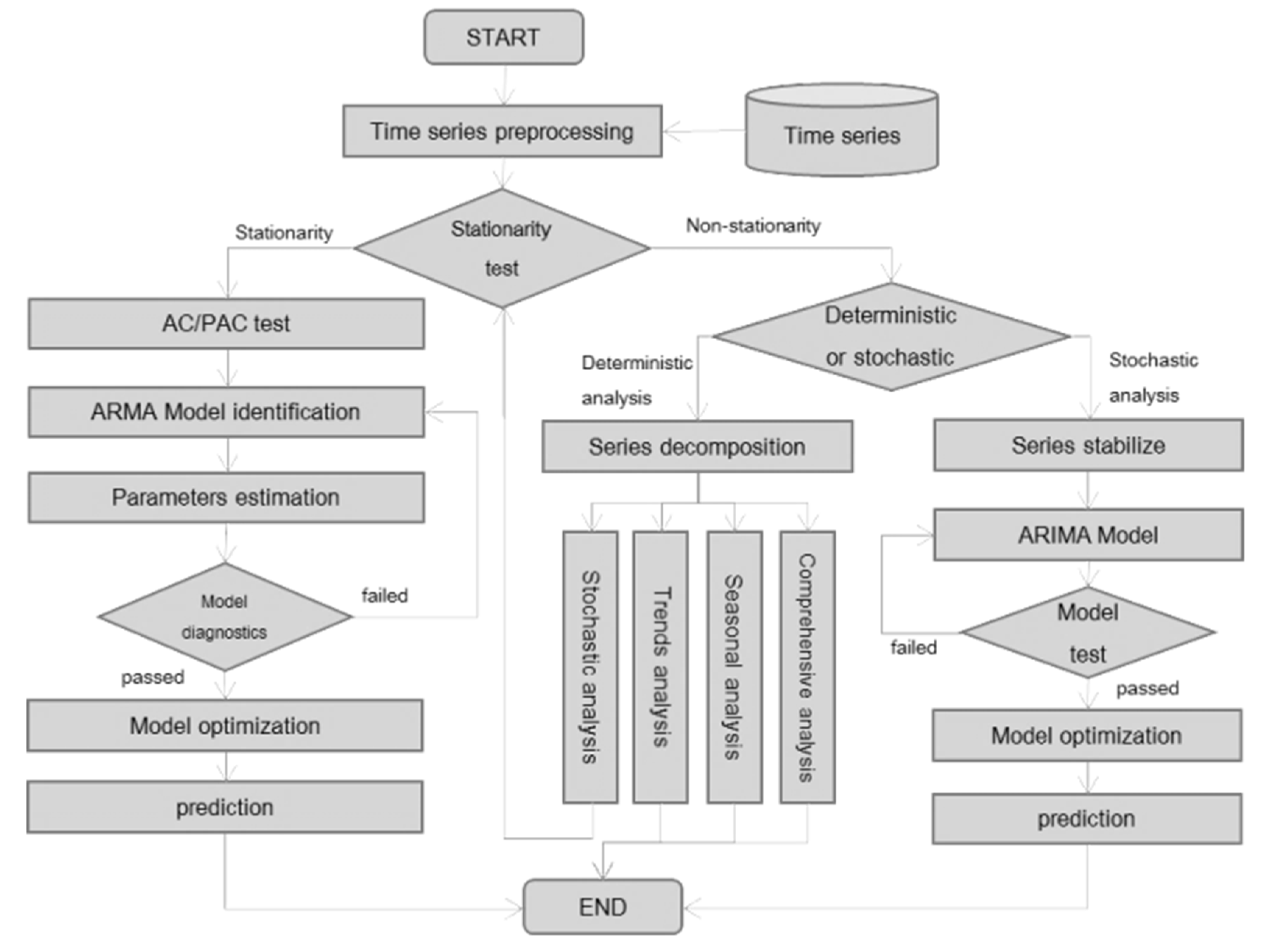
The widely used time series analysis methods can be categorized into two types: general descriptive time series analysis method and statistical time series analysis method [30]. Based on different data processing methods, the statistical time series analysis methods can be classified into the time domain and the frequency domain analysis methods [31]. The time-domain analysis methods are mainly used in short-term passenger flow prediction, and the main modeling steps are shown in Figure 1.
A stationary time series with autocorrelation characteristics can be analyzed by using time domain models, such as (autoregressive process with order ), (moving average process with order ), and (autoregressive moving average process with orders and ) [32].
Identifying a proper model to analyze a stationary time series is probably the most difficult task in practice. The orders of the autoregressive and moving average terms, need to be obtained before applying a model [33]. The autocorrelation coefficient functions and partial autocorrelation coefficient functions (ACF and PACF), used to examine the stationary data, will appear different features in figures of AR model, MA model and ARMA model, respectively, the general rules that are applied in interpreting these two functions are shown in Table 4 [33].
The next step is to estimate the parameters of the selected model. The most common methods are moment estimation, least squares estimation, maximum likelihood estimation, etc. The parameter estimation can be processed automatically by using R.
For the non-stationary time series, using differential operation, it can be transferred to a stationary one. The autoregressive integrated moving average (ARIMA) model can be used to analysis a non-stationary sequence.
The main purpose of using the time series method is to predict the values of the sequence in the future time.
For the time steps prediction, based on history data , the variable in the future time step would be predicted. The time is the forecast origin and is the lead time. The symbol denotes the predictive value of , also called estimation value.
Based on minimum mean square error forecasting, Equation (10) can be proved:
where the estimation of is equal to conditional expectation of .
3.2.2. Applications of Time Series Method in Short-Term Bus Passenger Flow Prediction
The statistical data of the bus passenger flow has the nature characteristics of time series, so that some researchers propose methods based on ARMA or ARIMA model to predict or analyze the passenger flow variation at the bus stop or lines using the observation data.
Gu [34] uses the ARMA model to forecast the passenger flow in the short-term at a transportation hub station of Shanghai, the largest city in China. In this paper, the bus hub station, located in one of the key areas of Shanghai named Wujiaochang, is set to be the observation point to carry out the passenger flow survey. The survey period is five weeks, and the sampling interval is 10 min. After eliminating weekends, a total of 2575 observations have been obtained. The time series composed of rough observations has cyclical and slow attenuation trend. Using variance analysis method (ANOVA) to eliminate cyclical and trend phenomenon appearing in different weekdays and different time of one day, the authors obtain a stationary sequence. By drawing ACF and PACF figures of the sequence, the model ARMA(2,1) is selected to predict the hub station passenger flow. Compared with the real data, the prediction accuracy of the hub station is proved to be over 80%, which meets the needs of disseminating the passenger flow forecasting information to the public and supporting the hub station management of the operators. However, the hub station is the passenger distribution center, which is the intersection of several lines, and it is difficult to distinguish the directions of the passenger flow. Therefore, the prediction results cannot provide useful information to optimize or coordinate different lines’ scheduling.
Ma [35] and Xue [36] propose an interactive multiple model (IMM) based approach combining with time series methods to predict short-term passengers of bus lines. The source data is the transaction records collected from AFC system in the both literatures. The data is aggregated in equal time interval (30 min [35] and 15 min [36]) to compose a time series according to different bus lines. After correlation, periodicity and stationarity analysis, three temporal relevant pattern time series are obtained. Here, three time series are introduced based on [35] briefly. The first is weekly relevant pattern time series , which consists of data weeks before with the same time interval at the same weekday, where is passenger count at time interval for day . The second is daily relevant pattern time series , which consists of data days before with the same time interval. The third is hourly relevant pattern time series , which consists of data time intervals before at the same day. After the ACF and PACF examination, Ma [35] selects AR(3) for weekly time series, SARIMA(1,0,0)(0,1,0)7 for daily time series, and ARIMA(2,1,0) for hourly time series. Xue [36] selects ARMA(2,2) for weekly time series, SARIMA(2,0,3)(1,0,0)24 for daily time series, and ARIMA(2,1,0) for hourly time series. The models selected by Ma [35] and Xue [36] fully prove that the weekly time series is a stationary sequence, from which it is speculated that the passenger variation is similar in the same time interval on the same weekday. The daily model reveals the cyclical variation of the passenger flow at the same time interval of different weekday during a cycle of week. The hourly model shows the obvious variation trend of the passenger flow in successive time intervals, such as the peak and off-peak period. Different time series model with different sampling interval will reveal different variation rules of passenger flow and, depending on different factors effecting the passenger flow variation, the predicted results will be different. Both studies propose an IMM-based algorithm, which combined different models prediction result together, and output final prediction in order to match the different situation. The details of the IMM algorithm will be discussed in Section 5.
However, the transaction records from the AFC system is the only data source in Ma [35] and Xue [36], which means the passenger using cash will not be counted, and the transactions are only generated in the bus dwell period, so that the data aggregation method used in these studies will generate more irregular data.
3.3. Other Linear Models for Short-Term Bus Passenger Flow Prediction
In addition to the Kalman filter and time series analysis methods, some researchers use general linear regression [37] and the wavelet model [38] to predict short-term passenger flow.
Yang [37] uses the general linear regression method to predict the short-term passenger flow. The source data are transaction records from the AFC system, and aggregated by hours. Using the clustering method, the data with a similar variation trend is clustered, and corresponding regression equations are selected to predict the passenger flow trend. Comparing with the survey data, the significance test indices are over 0.8, which meets the bus scheduling operation requirements.
4. Nonlinear Methods for Short-Term Bus Passenger Flow Prediction
Generally, the longer the sampling time interval is, the more detail information will be lost, and the more stable the sequence will be. Contrarily, the shorter the predicting period is, the greater the factors will affect the passenger flow, which will lead to be more obvious stochasticity, uncertainty, and non-linear [12], and it is difficult to use linear regression prediction methods. In order to improve the accuracy, some researchers try to construct complex and comprehensive models to describe bus passenger flow variation based on artificial neural networks (ANN), support vector machines (SVM), etc.
4.1. Support Vector Machine Regression-Based Methods for Short-Term Passenger Flow Prediction
4.1.1. Support Vector Machine Regression
Support vector machine regression (SVR or SVMR) [39] is a special application of a support vector machine (SVM) for regression. SVM is a supervised learning model, originally designed for classification, and it only needs a small amount of training data to fit the classification boundary or hyperplane and, finally, obtain very good classification effects. In order to keep the good properties of fitting an effective hyperplane, based on the structural risk minimization principle, minimizing the risk of quadratic -non loss function, Vapnik [40] proposed a SVM used for estimating the regression function, which could be called support vector regression. For solving different problems, the SVR can be categorized into linear regression and non-linear regression.
(1) Linear SVR
Dataset is N-dimensional with l groups patterns, described as:
Let a regression function , where , , to be estimated by using training dataset . Function is moved around to include training patterns inside -insensitive tube. By the structural risk minimization (SRM) principle, the generalization accuracy is optimized by the regression function flatness, which is guaranteed on small , and then fitting function is moved to minimize the norm [41]. In order to cover the data outside the -insensitive tube, the optimization problem of finding the best fitting function could be moved to a convex quadratic optimization problem described as:
subject to:
This regression optimization problem is constructed by optimization theory based on the characteristics of SVM, the detail proof procedure could be found in [39]. Ancona [42] interprets the SVR based on the ε-insensitive tube from the perspective of SVM classification theory.
(2) Non-linear SVR
Non-linear SVR has the similar idea with non-linear SVM classification, which uses the kernel function k(xi,xj) = ϕ(xi) · ϕ(xj) to change a non-linear regression problem in a low-dimensional space to a linear regression problem in a higher dimensional space. The detailed proof can be found in [39,42]. There are different kinds of kernel functions, such as linear kernel, polynomial kernel, radial base function (RBF), and sigmoid kernel function, etc., used for creating models. More information about the kernel function can be found in [43], which introduces the kernel functions used in the SVM application completely.
4.1.2. Applications of SVR in Short-Term Bus Passenger Flow Prediction
Yang [44] proposes a SVR method based on affinity propagation (AP) to predict the short-term passenger flow of bus stops. The sample data of passenger number is manually collected every 10-min and grouped by weekly cycle. The authors use an AP clustering algorithm to divide the passenger flow observations into different cluster subsets based on different principles, such as two groups of weekday and weekend, or six groups of each weekday and weekend. The basic idea of using the AP method is to group the similar data samples in order to reduce the volatility of the data sequence. Different SVR models are established to predict the future trend of each subset sequence. The authors prove that classifying the data sequence could improve the forecasting accuracy.
Guo [45] adopts Least Squares Support Vector Machine Regression (LS-SVMR) to establish a short-term passenger flow prediction model. The difference between the SVR and LS-SVMR is that the former uses the inequality constraints, the latter uses the equality constraints [46], and described as:
In the LS-SVMR algorithm, a QP problem is transformed to solve a linear equation, and easy to compute Lagrange multiplier. The convergence speed of LS-SVMR algorithm is higher than SVR, but the prediction accuracy is weaker than SVR. Guo [45] sets bus stop A as the observation site and the sampling interval to be 5 min, and then uses manual methods to count the arrival passenger of stop A together with upstream and downstream adjacent stops by every seven days for a cycle. The RBF is selected as the kernel function to construct the LS-SVMR based prediction model. The instance given by the authors show that the mentioned three factors, the passenger flow of upstream and downstream, waiting passenger amount, historical data at the same period, may affect forecasting accuracy. If setting adjacent time interval parameter , the performance of the prediction model will be the best.
Generally, selecting a proper kernel function needs several times testing in order to improve the normalization and adaptive capability, more detail information about the multiple kernel learning methods can be found in [47,48,49]. Based on multiple kernel LS-SVMR, Deng [12] uses linear, RBF and sigmoid, three kinds of kernel functions to construct the weighted summation [48] multiple kernel function (where is the total number of the kernel functions, is the balance weighted coefficient), to predict the short-term passenger flow. The data source are the transaction records from the AFC system, and aggregated every 10 min. The training dataset is constructed by the same time interval on the same weekday of weeks before, the same time interval of days before, and the successional time intervals before the time interval intended to be predicted. The authors illustrated an example to prove that the prediction accuracy by using the multiple kernel functions is higher than a single kernel function.
4.2. Artificial Neural Network-Based Methods for Short-Term Passenger Flow Prediction
4.2.1. Artificial Neural Network
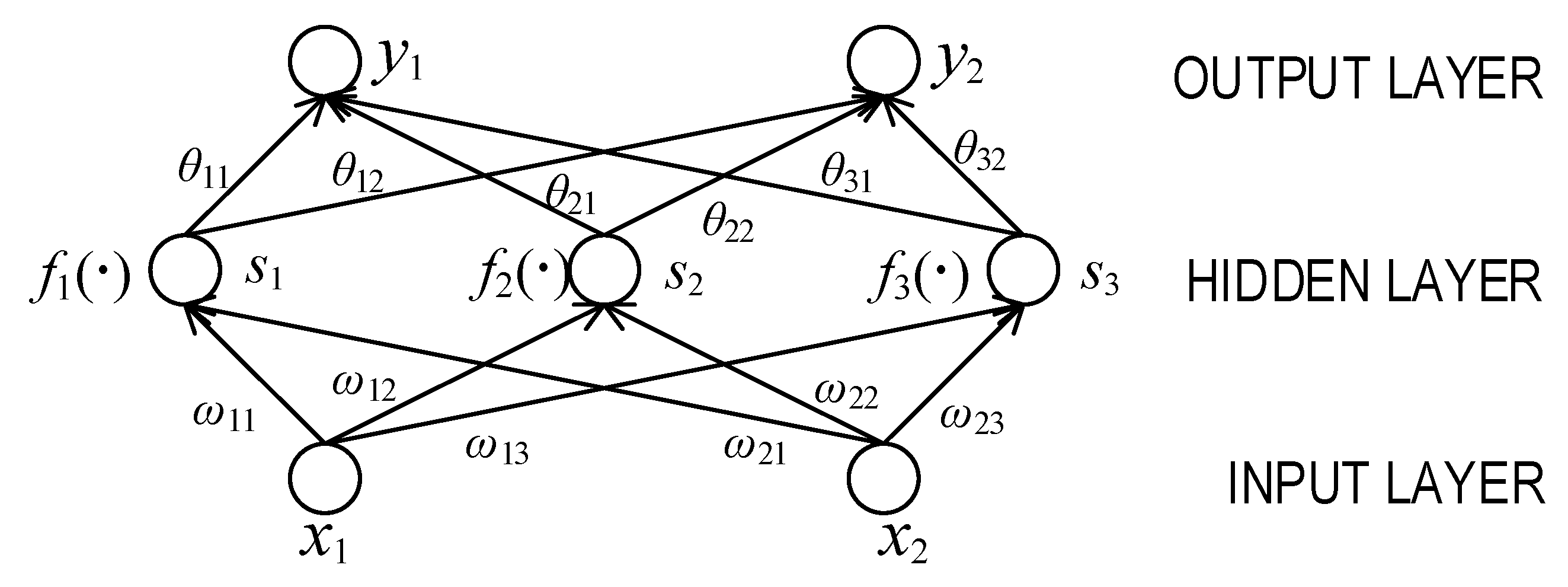
Artificial neural network (ANN) [50,51] is another non-linear regression method used in passenger flow prediction filed. The essential of ANN is a layered weighted directed graph [52], which can be divided into input layer, middle layer (or hidden layer) and output layer, and its structure is shown in Figure 2. The nodes in the directed graph are neurons, like , etc., and the directed edges are nerves.
In the ANN graph, the low layer nodes point to upper nodes by directed edges. The nodes in the same layer do not point to each other. The directed edge is usually assigned a weight, like , etc. The subscript of the weight represents the number of the neurons in different layer. Every neuron may have a linear or nonlinear function used for neuron transformation called neuron function. Take the neuron as an example, the value of may be described as . The input value is transferred upward layer by layer, and a more complex hyperplane could be constructed to forecast. Two components of the ANN need to be designed in the application, one is the network structure; the other is how to design the neuron functions . The categories of the ANN are generally classified by different network structures or neuron functions, such as BP-ANN [53], RBF-ANN [54], fuzzy ANN [55], etc.
4.2.2. Applications of ANN in Short-Term Bus Passenger Flow Prediction
In the earlier days, some researchers usually predicted the long-term passenger flow trend for days or years through ANN with manual survey data. For example, Yu [56] uses ANN to forecast the bus passenger trip flow between different city zones. Jiang [57] uses RBF-ANN and BP-ANN to predict the long-term passenger flow in one-year interval respectively, the results show the accuracy of RBF-ANN is better than BP-ANN. Yang [58] proposes a model based on the theory of adaptive neural fuzzy inference system to predict bus line passenger flow in day time interval. Compared with the AR and ARMA, the test results from the fuzzy ANN based model are better in accuracy. The time interval in days is not considered as short term anymore nowadays, but it plays an important guiding role in short-term bus passenger flow prediction, and the authors point out that the next step is to predict the passenger flow in hour interval based on the daytime interval prediction results.
Liu [59] proposes a model based on BP-ANN to predict passenger getting on and off flow at a bus stop. The authors select three layers BP-ANN to construct the predict model. The training data is divided into three groups as the model inputs. The first is the same period on the same weekday of the three weeks before the time prepared to be forecast. The second is the same period of the three days before the time prepared to be forecast. The last group is the three adjacent time intervals before the time prepared to be forecast. The total of 2608 samples are divided into three groups as BP-ANN inputs, compared with real data, the prediction accuracy is over 90%.
Lu [14] proposes a short-term passenger flow prediction model based on RBF-ANN. In this model, the data are transaction records from AFC system. The records with the same smart card ID ordered by transaction time are selected. The travel trace from origin to destination could be deduced according to the two adjacent records. From the travel trace information, the counts of boardings and alightings of passengers are obtained. Using the counts as the training data, the authors use RBF-ANN to predict the passenger flow at stops in one-hour interval. The literature does not describe the prediction process of RBF-ANN, but comparing with the real data, the absolute relative error of prediction results is less than 1.5%, which means the model has a certain value of practical application.
Wen [60] proposes a fuzzy ANN based real-time bus passenger flow forecast model. Different from other models, it uses similarity analysis to calculate the relationship between stop passenger flow distribution and line passenger flow distribution, and finds the key stops that affect the line passenger flow distribution. Based on the real-time passenger boarding counts from key stops, fuzzy ANN based model is used to forecast short-term passenger flow distribution of bus lines in one-hour intervals. The advantage of this model is to use similarity analysis to find key stops, which greatly reduces the cost of passenger flow survey, obtain better effective prediction results, and meet the precision requirements.
Dong [61] uses BP-ANN, improved BP-ANN and RBF-ANN to predict the passenger flow of the selected bus line by using the same transaction records from AFC system. The records are divided into three categories, the same as the input of the ANN in [59]. The results show that the accuracy of the improved BP-ANN and RBF-ANN are better than the traditional BP-ANN model.
4.3. Other Nonlinear Methods for Short-Term Passenger Flow Prediction
The grey model (GM) is widely used in bus passenger flow prediction filed. Liu [62] proposes a GM(1,1) model to predict short-term passenger flow of a bus line by using the transaction records from AFC system. The data are aggregated every 15 min and selected 10 consecutive Monday data in peak hour as training data. Compared with real data, the mean relative error of the prediction results is 3.343%, which means the accuracy of the prediction results is acceptable. Zhang [63] also uses GM(1,1) to predict the time-division passenger flow of a single line, and the relative residual of each group is less than 10%, which meet with the second order accuracy requirement. Shen [64] and Wang [65] declare that their research results are short-term prediction, but the prediction interval is over years, so that they are not considered as short-term prediction in this paper. However, the grey model deserves further study in the short-term bus passenger flow prediction field.
5. Combined Methods for Short-Term Bus Passenger Flow Prediction
Generally, the short-term passenger flow variation is more random and uncertain than the long-term passenger flow. It is hard to cover all characteristics of the short-term passenger flow by a single model. In order to make full use of the advantages of different models, researchers combine linear or nonlinear, different kinds of models together, to establish combination models. In this section, the combination models used for short-term passenger flow prediction are reviewed, and some combination models that deserve further study are simply introduced.
Gong [13] proposes a framework with three sequential stages, including a seasonal ARIMA-based method, an event-based algorithm and a Kalman filter-based algorithm, to predict the short-term passenger flow of bus stops. In the first stage, a time series method is used to predict the arrival passenger count (ArPC) and empty space count (ESC) of a bus. In the second stage, an event-based method is developed to predict the departure passenger counts (DPC) from the stop. In the third stage, a Kalman filter-based method is used to predict the waiting passenger count (WPC) according to the results from the first and second stages. The passenger boarding counts are collected from the APC or cameras installed in each bus. The WPC data is collected through cameras installed at each bus stop. The researchers suggest that the passenger flow of a bus stop is the waiting passenger at the bus stop, which is strongly related to bus arrival times and its current passenger capacity. Based on these principles, the WPC at a bus stop is represented mathematically as:
which means the count of passengers waiting at a bus stop at time relates to the count of passenger waiting at a bus stop at time , count of passenger arriving at the stop at time , and count of passenger departing from the stop at time . Based on the principle represented by (17), the ArPC and DPC need to be predicted before predicting WPC. The first stage is to predict the ArPC. The authors analyze the relation between the passenger boarding count data and arriving data, and proposed a passenger allocation approach to compute the historical ArPC. The boarding count can be collected through the APC. While the passenger arrival process is treated as a Poisson distribution with the probability density function . The ArPC at time can be presented as:
where is the time of ith bus arrival event and is history data of boarding count. Using (18), the historical ArPC data will be obtained, and the data repeat in a week-cycle pattern. According to the ACF and PACF experiments, ARIMA(1,0,0)(1,0,0)7 model is selected to predict ArPC and ESC. Compared with real data, the average relative errors of prediction results are 2.94% of ArPC and 3.02% of ESC. The second stage is to predict the DPC, which is triggered by the bus arrival events (BAEs) at a bus stop in each time interval. Under the author’s assumption, the boarding count of BAE is the minimum of the passengers waiting at the stop and the empty space available on the bus. The boarding count is collected from the APC, so the DPC is the sum of the boarding count of every BAE happened during the time interval . Therefore, predicting DPC is equivalent to predicting the BAEs at the corresponding stop. Using bus trajectory records from the AVL, an event-based algorithm is proposed to predict the bus arrival time, and combining with the predict results of ArPC and ESC in the first step, the DPC can be predicted. The third stage has been discussed in the previous section. At the end of the literature, a numerical experiments conducted at three typical bus stops are illustrated to demonstrate that the proposed framework is robust and accurate.
Ma [35] and Xue [36], discussed in Section 3.2.2, propose weekly, daily and hourly three temporal relevant pattern time series to predict passenger flow on the bus lines. The three patterns select AR (ARMA), SARMA and ARIMA separately to capture different characteristics of time series. In order to maximize the advantages of single models and optimize the interaction between them, the two literatures propose an IMM-based algorithm to combine the predictions of each single model. The output equation of the IMM is defined as:
where is the prediction result of model at time ; is the mixed probability. The IMM-based algorithm is a recursive approach, including four steps: re-initialization, model filtering, probability updating and hybrid output. The first step is to calculate the mixed state and covariance at time based on transition matrix with the updated estimations and probabilities from the last recursive. The second step is using Kalman filter algorithm to update the estimations for each model, and calculate the residual and covariance with the input of real-time measurement. The third step is updating the probability of each model at time based on likelihood function of each model. The fourth step is calculating the final estimation at time weighted by the updated probability [35]. The IMM algorithm combines the weekly, daily and hourly time series models to match different data states in order to reduce the errors of using one single model. Comparing with single models, the IMM-based hybrid model can provide more accurate prediction results.
Liu [38] proposes a short-term passenger flow forecasting method by combining the wavelet and time series. Its basic idea is to treat the observation sequences of the passenger flow as the timing signals. Using discrete Flourier transformation (DFT) converts the time domain of the original sequence to frequency domain. Using Mallat-based wavelet decomposition method divides the changed sequence into one low frequency main trend signal and five high frequency interference signals. Comparing with the original sequence, the single signal sequence is more stationary. The ARMA model is used to predict the future trend of each series. Finally, the wavelet reconstruction method is used to synthesize these single prediction results together as the final prediction result. From the authors’ view, the wavelet decomposition and reconstruction method reduce the volatility of the original signal. Therefore, the wavelet prediction method can improve the forecast accuracy effectively. However, the original sequence is not stationary, the conclusion of ARMA(4,4) model, used to prove the proposed wavelet method with higher forecast accuracy, needs to be confirmed by further research.
Zhou [66] proposes a sliding window ensemble framework to predict the short-term passenger flow. The framework includes three distinct predicting models. The first is the time varying Poisson model, which is used to predict the average number of passenger demand in a fixed time period. The second is the weighted time varying Poisson model, which is to predict the passenger flow with seasonal burst issues. The third one is using ARIMA model to predict the short-term passenger flow. The three models could use long, medium and short-term historical data as training data respectively, and be combined together to improve prediction result by:
where M = {M1, M2, … Mz} is the set of z models of interest to model a given time series and Mt = {M1t, M2t, … Mzt} is the set of prediction values of the next period in the time interval t by those models. PiH is the forecasting accuracy of the model Mi in the time window [t − H, t]. The prediction results show that the accuracy of the ensemble framework is around 79%, which is better than the single models. The ensemble framework in [66] is used to develop a prototype APP for mobile phone users to predict the crowdedness of the bus.
Liu [67] proposes a combined predicting model with BP-ANN and LS-SVM. The combined model includes two steps: firstly, the BP-ANN is adopted to do an initial prediction with the historical training data, and then the LS-SVM is used to refine the initial prediction. The result shows the combination model can improve the prediction accuracy by 1% more than single model. From the authors’ perspective, the proposed model combines the advantages of the nonlinear fitting ability of BP-ANN and using small amount training data of LS-SVM, which may improve the prediction accuracy.
Pekel [68] develops two hybrid model, parliamentary optimization algorithm-artificial neural network (POA-ANN) and intelligent water drops algorithm-artificial neural network (IWD-ANN), POA and IWD are utilized to optimize the number of the hidden layer neurons and weight of hidden layer neurons, so as to make global optimization of the model.
Some researchers propose different combined methods used to predict bus passenger flow, such as combining with different linear regression functions together, combining the grey model with ANN, the grey model with Markov, etc. However, these methods are used for predicting long-term, years’ or months’ interval, passenger flow. Here, these methods are introduced simply, the basic idea of which deserves further study. Gan [69] gives a combined method with three weighted linear regression to predict the bus line passenger flow. Ge [70] proposes a combined method based on genetic algorithm and ANN, and Cai [71] proposes a similar model by combing genetic algorithm and BP-ANN, which used genetic algorithm to define data weight of initial input. The grey model (GM) is widely used to construct combined models with others, such as Yang [72] and Shen [64], who propose a similar combination prediction method based on GM and Markov models. Wang [65] proposes a random grey ant colony neural network combined model with random grey model and recurrent neural network. Ling [73] uses the sum of the absolute values of the predicted sequence and residual sequence to construct a new sequence as the input of GM(1,1) to predict the passenger flow.
6. Big Data Technology and Deep Learning Used for Short-Term Bus Passenger Flow Prediction
The short term bus passenger flow prediction technology is urgently needed by the bus companies, but it develops very slowly. One of the reasons leading to slow its development is that it is hard to obtain the information about passenger flow. Traditional manual survey to collect data costs much time, and it does not suit for short-term passenger flow prediction. Until recent years, it is possible to collect the passenger flow data in real-time with the help of APTS. Since then, the literatures, proposed methods to predict short-term passenger flow, usually used the data from AFC or APC. Another problem is that too much data is collected in short term. Such as the AFC system used in Beijing, the transaction records are over 10 million per day, and the traditional methods hardly handle these data in time. Thanks to the big data technology, storing and accessing a very large amount data are no longer significant problems.
Li [74] uses the MapReduce to implement the BP-ANN parallel algorithm. There are two kinds of parallel approaches to implement the algorithm, one is the structure parallel, and the other is training data parallel. The second approach is very suitable for the big data technology, because the basic idea of the MapReduce technology is to divide the data file into small pieces, and used different machines to speed up the training data process. Li [74] uses data parallel approach to train the BP-ANN, and exchange the training results through a unified weight list table. Comparing with the traditional BP-ANN, the training time spent by the MapReduce-based algorithm is one-sixth of the traditional algorithm and the prediction accuracy is almost the same.
Deep learning, successfully applied in many fields and achieved amazing results, can deeply and abstractly extract the nonlinear features embedded in the dataset, that are attracting some researchers using deep learning to predict the short-term passenger flow variation.
Liu [75] proposes an unsupervised training model based on a stacked autoencoder (SAE) combined with a supervised training model based on deep neural network (DNN) to predict hourly passenger flow. Passenger flow data are collected from the AFC for four months. The authors explain why the hidden nodes can robustly extract and represent the valuable features embedded in the input data by visualizing the high-level features learned in different hidden layers. The experimental results show that the selections and combinations of the input features have a great impact on the accuracy of the prediction results. The highest average RMSE is 75% across all of scenarios, however, the authors believe that it is a universal and robust hourly passenger flow prediction model.
7. Conclusions
In this paper, more than 20 studies about bus passenger flow prediction are discussed. Twenty-two pieces of literature, listed in Table 5 and Table 6, about short-term bus passenger flow prediction are discussed briefly, and the rest about long-term bus passenger flow prediction deserving further study are introduced simply. In the two tables, the characteristics and the evaluation of the methods used by each paper are also listed.
Table 5 lists the single linear and nonlinear methods for short-term passenger flow prediction. From the column of “Accuracy”, the accuracy of nonlinear method is better than the linear method. For the modeling difficulty, time series and linear regression methods are easier than nonlinear models. The structures of training datasets or sample datasets used as the input of the model are relatively simple, most of which are original time sequence data or roughly processed data. Therefore, it is easy to use single models to predict the passenger flow, and obtain relatively satisfactory prediction results with low cost.
Table 6 lists the combination model used for short-term passenger flow prediction. The first four literatures propose methods by combining different types of time series methods together to handle different situation of the sample datasets, which are carefully designed and selected from the rough data sequence. Therefore, the complexity of the dataset structure and the modeling process is very high, which leads to weaken universality of the combined model. The accuracy of the combination models is better than the single model, but the cost is higher.
From the tables listed below, the nonlinear models and combination models are better in prediction accuracy, but the complex modeling process will make the computational complexity higher, and well-defined data structures will cost more time to preprocess rough data, so that if the time costs more than prediction period, the method will lose meaning. Liu [67] proposes the comparison of the computing speed between different methods. In the short-term prediction field, the speed will be more important than accuracy, especially for the APTS equipped in buses, which produced a very large amount of data needing to be treated in time. It is valuable to improve the traditional prediction models by using big data technology so as to accelerate the computing speed.
Since there is no complete experiment dataset given by the authors of the references in this paper, and the evaluating criteria is also not uniform, it is difficult to evaluate the methods or models objectively. In further study, all prediction methods mentioned in the references will be tested and comparatively analyzed, using a unified data source under the unified evaluating criteria,
The urban bus transit system plays an important role in the public transit services, and its service ability has been paid close, extensive attention. However, traffic jams, weather conditions, even irregular business activities, will cause sudden changes of the passenger flow. Overcrowded carriages or long waiting times will cause passengers to be dissatisfied with the quality of the bus service. As discussed earlier, passenger flow is the basis of public transport operation. Bus operators hope to improve the quality of bus services to increase corporate profits by developing flexible timetables based on short-term passenger flow changes. Due to the difficulties in obtaining real-time passenger flow statistics for a long time, related applications based on short-term passenger flow changes cannot be applied in practice. With the widespread use of APTS equipment, it is now possible to obtain passenger flow statistics in real-time, and application research based on short-term passenger flow changes has been rapidly developed. DiDi, the largest Chinese ride-sharing company, has launched a shared bus system based on real-time passenger flow demand, which comprehensively considers the number of passengers, travel demand, traffic conditions, and other factors to plan routes in real-time and dispatch buses to meet diverse public travel needs. In future work we will cooperate with a large-scale bus operation enterprise to develop a bus fleet intelligent dispatching operation platform based on short-term passenger flow changes, helping the enterprise to optimize the timetables and subsequent bus fleet and crew scheduling. At the same time, the bus fleet operation information release platform is provided, and the bus arrival information is pushed through the electronic station plate or mobile terminal APP, so as to help the travelers to reasonably arrange the travel plan and improve the bus service level.
Author Contributions
H.Z. conceived the research, proposed the original idea, and wrote most of the paper. L.C. and Y.N. proposed some original idea of the research and wrote some parts of the research. X.X. and W.Z. gave related guidance.
Acknowledgments
This work was supported by Fundamental Research Funds for the Central Universities (Grant No. 3132016308, 3132018197) and Liaoning Provincial Natural Science Foundation of China (Grant No. 20170520196).
Conflicts of Interest
The authors declare no conflict of interest.
References
- Rizzi, L.I.; De La Maza, C. The external costs of private versus public road transport in the metropolitan area of Santiago, Chile. Transp. Res. Part A Policy Pract. 2017, 98, 123–140. [Google Scholar] [CrossRef]
- Vuchic, V.R. Urban public transportation systems. In Transportation Engineering and Planning; EOLSS: Paris, France, 2002; Volume 1. [Google Scholar]
- Suman, H.K.; Bolia, N.B.; Tiwari, G. Comparing public bus transport service attributes in Delhi and Mumbai: Policy implications for improving bus services in Delhi. Transp. Policy 2017, 56, 63–74. [Google Scholar] [CrossRef]
- Land Transport Authority Academy. Passenger Transport Mode Shares in World Cities. Journeys 2011, 11, 54–64. [Google Scholar]
- Moretti, L.; Moretti, M.; Ricci, S. Upgrading of Florence public transport to incorporate new tramlines. Ing. Ferrov. 2017, 72, 568–584. [Google Scholar]
- Ceder, A. Public Transit Planning and Operation: Modeling, Practice and Behavior; CRC Press: Boca Raton, FL, USA, 2015. [Google Scholar]
- Vuchic, V.R. Urban Transit: Operations, Planning, and Economics; John Wiley & Sons: New York, NY, USA, 2017. [Google Scholar]
- Loprencipe, G.; Moretti, M.; Moretti, L.; Ricci, S. Rail accessibility to a planned new soccer stadium in Rome. Ing. Ferrov. 2017, 72, 287–305. [Google Scholar]
- Noekel, K.; Viti, F.; Rodriguez, A.; Hernandez, S. Modelling Public Transport Passenger Flows in the Era of Intelligent Transport Systems; Gentile, G., Noekel, K., Eds.; Springer Tracts on Transportation and Traffic; Springer International Publishing: Cham, Switzerland, 2016; Volume 1, ISBN 978-3-319-25080-9. [Google Scholar]
- Hwang, M.; Kemp, J.; Lerner-Lam, E.; Neuerburg, N.; Okunieff, P.; Schiavone, J. Advanced Public Transportation Systems: The State of the Art Update 2006; U.S. Federal Transit Administration: Washington, DC, USA, 2006.
- Lehman Center for Transportation Research. Florida Advanced Public Transit Systems Program; Lehman Center for Transportation Research: Miami, FL, USA, 2009. [Google Scholar]
- Deng, H.; Zhu, X.; Zhang, Q.; Zhao, J. Prediction of short-term public transportation flow based on multiple-kernel least square support vector machine. J. Transp. Eng. Inf. 2012, 10, 84–88. [Google Scholar]
- Gong, M.; Fei, X.; Wang, Z.; Qiu, Y. Sequential framework for short-term passenger flow prediction at bus stop. Transp. Res. Rec. J. Transp. Res. Board 2014, 2417, 58–66. [Google Scholar] [CrossRef]
- Lu, B.; Deng, J.; Ma, Q.; Liu, Q.; Zhang, K. A short-term public transit volume forecasting model based on IC Card and RBF neural network. J. Chongqing Jiaotong Univ. Sci. 2015, 34, 106–110. [Google Scholar]
- Ying, L.; Lijun, S.; Sui, T. A review of urban studies based on transit smart card data. Urban Plan. Forum 2015, 3, 70–77. [Google Scholar] [CrossRef]
- Pelletier, M.-P.; Trépanier, M.; Morency, C. Smart card data use in public transit: A literature review. Transp. Res. Part C Emerg. Technol. 2011, 19, 557–568. [Google Scholar] [CrossRef]
- Wade, R. Public Transportation Prices in 80 Worldwide Cities; Price of Travel: Los Angeles, CA, USA, 2017. [Google Scholar]
- Jiang, M. Analysis on the Subway with Bus Transfer Time Based on IC Card Data. Master’s Thesis, Southeast University, Nanjing, Jiangsu, China, 2015. [Google Scholar]
- Kotz, A.J.; Northrop, W.F.; Kittelson, D.B. Automated Passenger Counter Systems and Methods. US Patent 20170057316A1, 31 August 2015. [Google Scholar]
- Jose, D.; Prasad, S.; Sridhar, V.G. Intelligent vehicle monitoring using global positioning system and cloud computing. Procedia Comput. Sci. 2015, 50, 440–446. [Google Scholar] [CrossRef]
- Kalman, R.E. A new approach to linear filtering and prediction problems. J. Basic Eng. 1960, 82, 35. [Google Scholar] [CrossRef]
- Welch, G.; Bishop, G. An Introduction to the Kalman Filter; UNC: Chapel Hill, NC, USA, 2006; Volume 7, pp. 1–16. [Google Scholar]
- Zhang, C.; Song, R.; Sun, Y. Kalman filter-based short-term passenger flow forecasting on bus stop. J. Transp. Syst. Eng. Inf. Technol. 2011, 11, 154–159. [Google Scholar]
- Grewal, M.S. Kalman Filtering. In International Encyclopedia of Statistical Science; Lovric, M., Ed.; Springer: Berlin/Heidelberg, Germany, 2011; pp. 705–708. ISBN 978-3-642-04898-2. [Google Scholar]
- Grewal, M.S. Kalman Filtering Theory and Practice Using MATLAB; John Wiley & Sons, Inc.: Hoboken, NJ, USA, 2015; Volume 1, ISBN 978-8-578-11079-6. [Google Scholar]
- Chui, C.K.; Chen, G. Kalman Filtering: With Real-Time Applications; Springer Science and Business Media: Berlin, Germany, 2009; ISBN 978-3-540-87848-3. [Google Scholar]
- Chatfield, C. The Analysis of Time Series: An Introduction, 6th ed.; Chapman and Hall/CRC Press: Boca Raton, FL, USA, 2003; Volume 140, ISBN 1-58488-317-0. [Google Scholar]
- Brockwell, P.J.; Davis, R.A. Introduction to Time Series and Forecasting; Springer Science & Business Media: Berlin, Germany, 2006; ISBN 0-38721657X. [Google Scholar]
- Cochrane, J.H. Time Series for Macroeconomics and Finance; University of Chicago: Chicago, IL, USA, Unpublished Manuscript; pp. 1–136.
- Wang, Y. Applied Time Series Analysis, 4th ed.; China Renmin University Press: Beijing, China, 2015. [Google Scholar]
- Brandes, O.; Farley, J.; Hinich, M.; Zackrisson, U. The time domain and the frequency domain in time series analysis. Swedish J. Econ. 1968, 70, 25–42. [Google Scholar] [CrossRef]
- Kirchgässner, G.; Wolters, J. Introduction to Modern Time Series Analysis, 2nd ed.; Springer: Berlin/Heidelberg, Germany, 2013; ISBN 978-3-540-73290-7. [Google Scholar]
- Washington, S.P.; Karlaftis, M.G.; Mannering, F.L. Statistical and Econometric Methods for Transportation Data Analysis, 2nd ed.; Chapman and Hall/CRC Press: Boca Raton, FL, USA, 2011; ISBN 1584880309. [Google Scholar]
- Gu, Y.; Han, Y.; Fang, X. Method of hub station passenger flow forecasting based on ARMA model. J. Transp. Inf. Saf. 2011, 29, 5–9. [Google Scholar]
- Ma, Z.; Xing, J.; Mesbah, M.; Ferreira, L. Predicting short-term bus passenger demand using a pattern hybrid approach. Transp. Res. Part C Emerg. Technol. 2014, 39, 148–163. [Google Scholar] [CrossRef]
- Xue, R.; Sun, D.J.; Chen, S. Short-term bus passenger demand prediction based on time series model and interactive multiple model approach. Discret. Dyn. Nat. Soc. 2015, 2015. [Google Scholar] [CrossRef]
- Yang, Z.; Zhao, Q.; Zhao, S.; Jin, L.; Mao, Y. Passenger flow volume forecasting method based on public transit Intelligent Card (IC) survey data. Transp. Stand. 2009, 196, 115–118. [Google Scholar]
- Liu, K.; Li, W.; Zhao, J. Study on wavelet forecast method for short-term passenger flow. J. Transp. Eng. Inf. 2010, 8, 111–117. [Google Scholar]
- Smola, J.; Scholkopf, B. A tutorial on support vector regression. Stat. Comput. 2004, 14, 199–222. [Google Scholar] [CrossRef] [Green Version]
- Vapnik, V.N. The Nature of Statistical Learning Theory; Springer: Berlin/Heidelberg, Germany, 1995; Volume 8, ISBN 0387945598. [Google Scholar]
- Kim, D.; Cho, S. ε-Tube based pattern selection for support vector machines. In Proceedings of the Pacific-Asia Conference on Knowledge Discovery and Data Mining, Singapore, 9–12 April 2006; Springer: Berlin/Heidelberg, Germany, 2006; pp. 215–224. [Google Scholar]
- Ancona, N. Properties of Support Vector Machines for Regression; Technical Report; Center for Biological and Computational Learning, Massachusetts Institute of Technology: Cambridge, MA, USA, 1999. [Google Scholar]
- Scholkopf, B.; Smola, A.J. Learning with Kernels: Support Vector Machines, Regularization, Optimization, and Beyond; MIT Press: Cambridge, MA, USA, 2002; ISBN 0262194759. [Google Scholar]
- Yang, X.; Liu, L. Short-term passenger flow forecasting on bus station based on affinity propagation and support vector machine. J. Wuhan Univ. Technol. Sci. Eng. 2016, 40, 36–40. [Google Scholar]
- Guo, S.; Li, W.; Bai, W.; Zhang, D. Prediction of short-term passenger flow on a bus stop based on LSSVM. J. Wuhan Univ. Technol. Sci. Eng. 2013, 37, 603–607. [Google Scholar]
- Wang, H.; Hu, D. Comparison of SVM and LS-SVM for regression. In Proceedings of the International Conference on Neural Networks and Brain (ICNN), Beijing, China, 13–15 October 2005; Volume 1, pp. 279–283. [Google Scholar]
- Gönen, M.; Alpaydın, E. Multiple kernel learning algorithms. J. Mach. Learn. Res. 2011, 12, 2211–2268. [Google Scholar]
- Wang, H.-Q.; Sun, F.-C.; Cai, Y.-N.; Chen, N.; Ding, L.-G. On multiple kernel learning methods. Acta Autom. Sin. 2010, 36, 1037–1050. [Google Scholar] [CrossRef]
- Lanckriet, G.; Cristianini, N. Learning the kernel matrix with semidefinite programming. J. Mach. Learn. Res. 2004, 5, 27–72. [Google Scholar]
- Jain, A.K.; Mao, J.; Mohiuddin, K.M. Artificial neural networks: A tutorial. Computer 1996, 29, 31–44. [Google Scholar] [CrossRef]
- Haykin, S. Neural Networks and Learning Machines; Prentice Hall: Upper Saddle River, NJ, USA, 2008; Volume 3, ISBN 9780131471399. [Google Scholar]
- Wu, J. Beauty of Mathematics, 2nd ed.; Posts and Telecom Press: Beijing, China, 2012; Volume 1, ISBN 9787115282828. [Google Scholar]
- Hecht-Nielsen, R. Theory of the backpropagation neural network. In Proceedings of the International 1989 Joint Conference on Neural Networks, Washington, DC, USA, 18–22 June 1989; Volume 1, pp. 593–605. [Google Scholar] [CrossRef]
- Bishop, C.M. Improving the generalization properties of radial basis function neural networks. Neural Comput. 1991, 3, 579–588. [Google Scholar] [CrossRef]
- Buckley, J.J.; Hayashi, Y. Fuzzy neural networks: A survey. Fuzzy Sets Syst. 1994, 66, 1–13. [Google Scholar] [CrossRef]
- Yu, S.; Shang, C.; Yu, Y.; Zhang, S.; Yu, W. Prediction of bus passenger trip flow based on artificial neural network. Adv. Mech. Eng. 2016, 8. [Google Scholar] [CrossRef] [Green Version]
- Jiang, P.; Shi, Q.; Chen, W.; Zhang, W. Forecast of passenger volume based on neutral network. J. Wuhan Univ. Technol. Sci. Eng. 2009, 33, 414–417. [Google Scholar]
- Yang, X.; Wang, W.; Gu, W.; Zhou, M. Applying fuzzy neural network to predict bus line passenger flow. J. Highw. Transp. Res. Dev. 2000, 17, 38–40. [Google Scholar]
- Liu, C.; Zhang, Y.; Zhang, H. Transit station’s temporal getting on/off flow forecasting model based on BP neural network. Commun. Stand. 2008, 177, 186–189. [Google Scholar]
- Wen, H.; Wang, X.; Rong, L.; Chen, X. Real-time forecast for passenger flow of bus based on fuzzy neural network. Microcomput. Inf. 2009, 12, 225–226. [Google Scholar] [CrossRef]
- Dong, H. Real-time Analysis and Short-term Forecast of Bus Passenger Flow. Master’s Thesis, Dalian University of Technology, Dalian, Liaoning, China, 2013. [Google Scholar]
- Liu, Y. Grey Model Based Temporal Passenger Flow Prediction with IC Card Records. Master’s Thesis, Shandong University, Jinan, Shandong, China, 2011. [Google Scholar]
- Zhang, Z.; Xu, X.; Wang, Z. Application of grey prediction model to short-time passenger flow forecast. In AIP Conference Proceedings; American Institute of Physics: College Park, MD, USA, 2017; Volume 1839, p. 20136. [Google Scholar]
- Shen, J.; Wang, W.; Chen, J. Short-term urban public transit volume forecast based on gray-markov model. J. Highw. Transp. Res. Dev. 2007, 24, 120–123. [Google Scholar]
- Wang, Q.; Zhang, Q. Forecasting of short-term urban public transit volume based on random gray ant colony neural network. Appl. Res. Comput. 2012, 29, 2078–2080. [Google Scholar]
- Zhou, C.; Dai, P.; Li, R. The passenger demand prediction model on bus networks. In Proceedings of the IEEE 13th International Conference on Data Mining Workshops, ICDMW 2013, Dallas, TX, USA, 7–10 December 2013; pp. 1069–1076. [Google Scholar]
- Liu, J.; Heng, Y.; Zhao, H.; Gao, X.; Wang, P. A prediction model of short-term passenger flow for urban transit hubs. J. Transp. Inf. Saf. 2014, 32, 41–44. [Google Scholar]
- Pekel, E.; Kara, S.S. Passenger flow prediction based on newly adopted algorithms. Appl. Artif. Intell. 2017, 31, 64–79. [Google Scholar]
- Gan, W.; Kong, J. Study of combine-forecast method for passenger volume of urban public transit system. Sci. Mosaic 2011, 2, 106–108. [Google Scholar] [CrossRef]
- Ge, L.; Wang, W.; Deng, W.; Shan, X. Research on practical forecast method of passenger volume for urban public transport hub. J. Highw. Transp. Res. Dev. 2005, 22, 110–113. [Google Scholar]
- Cai, Z. Research on Prediction of Conventional Public Transit Passengers’ Volume in Small and Medium Sized Cities Based on Neural Networks. Master’s Thesis, Southwest Jiaotong University, Chengdu, Sichuan, China, 2013. [Google Scholar]
- Yang, Q.; Yang, Y.; Feng, Z.; Zhao, X. Prediction method of passenger volume of city public transit based on grey theory and markov model. China J. Highw. Transp. 2013, 26, 169–175. [Google Scholar]
- Ling, H.; Xi, E. Prediction model of public transport passenger volume based on random fluctuations. J. Chang. Univ. Natural Sci. Ed. 2012, 32, 85–88. [Google Scholar]
- Li, Z. Research of Bus Passenger Flow Analysis and Prediction Based on Hadoop. Master’s Thesis, Northeast Normal University, Changchun, Jilin, China, 2015. [Google Scholar]
- Liu, L.; Chen, R.-C. A novel passenger flow prediction model using deep learning methods. Transp. Res. Part C Emerg. Technol. 2017, 84, 74–91. [Google Scholar] [CrossRef]
Figure 1.
Time-domain series modeling steps.

Figure 2.
Artificial neural network (ANN) diagram.


Table 1.
The structure of the transaction record.
| Field Name | Illustration |
|---|---|
| Card ID | The unique number of the smart card |
| Type of smart card | Normal card, coupon card, etc. |
| Driver ID | The unique number of the current bus driver |
| Line ID | The unique number of the bus line |
| Vehicle ID | The unique number of the vehicle |
| Balance | The balance of the smart card after the last transaction |
| Transaction amount | The transaction amount of the last transaction |
| Transaction count | The total number of the transaction count with this smart card |
| Transaction time | The time of the last transaction |
Table 2.
The structure of the record from the automatic passenger counters (APC).
| Field Name | Illustration |
|---|---|
| Equipment ID | The unique number of the equipment |
| On/off | Denotes the passenger getting on or off the bus |
| Vehicle ID | The unique number of the vehicle |
| Line ID | The unique number of the bus line |
| Trip type | Denotes the current trip is up run or down run |
| Stop ID | The unique number of stops, where the bus stops at the current time |
| Count time | The time when the passenger scans through the AFC |
| Stop accumulation | The total number of the passengers getting on or off at a stop |
Table 3.
The structure of the record from the vehicle intelligent terminal system.
| Field Name | Illustration |
|---|---|
| Equipment ID | The unique number of the vehicle intelligent terminal system |
| Vehicle ID | The unique number of the vehicle |
| Driver ID | The unique number of the driver |
| Longitude | The longitude of the current vehicle position |
| Latitude | The latitude of the current vehicle position |
| Speed | The vehicle real-time speed |
| Heading | The vehicle heading direction at the current time |
| Line ID | The unique number of the bus line |
| Stop ID | The unique number of stop, where the bus stops at the current time |
| Distance | The relative distance from the current position to the last station |
| Cumulative distance | The total mileage of the vehicle |
| State | The state of the vehicle intelligent terminal system |
Table 4.
ACF and PACF behavior for the ARMA model.
| Categories | AR(p) | MA(q) | ARMA(p, q) |
|---|---|---|---|
| ACF | Tails off exponentially | Cuts off after lag q | Tails off exponentially |
| PACF | Cuts off after lag p | Tails off exponentially | Tails off exponentially |
Table 5.
Single models about short-term bus passenger flow prediction.
| Author(s) | Method | Contrast Method | Method Style | Predict Object | Data Source | Data Structure a | Modeling Difficulty b | Universality of Model c | Accuracy |
|---|---|---|---|---|---|---|---|---|---|
| Zhang (2011) [23] | Kalman filter | BP-ANN | Single | Stop | AFC Video | Simple | Complex | Weak | around 80% |
| Gu (2011) [34] | ARMA(2,1) | GM(1,1) | Single | Hub | Manual survey | Simple | Easy | Middle | around 80% |
| Yang(2009) [37] | Linear regression | Real data | Single | Line | AFC | Complex | Easy | Weak | NA |
| Yang (2016) [44] | AP(6) based SVM | AP(p) based SVM | Single | Stop | Manual survey | Complex | Low complexity | Middle | Over 85% |
| Guo (2013) [45] | LSSVM | LSSVM with different factors | Single | Stop | Manual survey | Low complexity | Low complexity | Weak | MAE 0.625 MSE 0.9145 |
| Deng (2012) [12] | Multiple kernel LSSVM | Single kernel LSSVM | Single | Stops | AFC | Simple | Low complexity | Middle | EC 0.9544 |
| Yang (2000) [58] | Fuzzy ANN | AR ARMA | Single | Line | Manual survey | Low complexity | Low complexity | Weak | ME 7.47% |
| Liu(2008) [59] | BP-ANN | Real data | Single | Stops | NA | Low complexity | Low complexity | Middle | EC 0.901 |
| Lu(2015) [14] | RBF-ANN | Real data | Single | Stops | AFC | Simple | Low complexity | High | ME/MSE less 1.5% |
| Wen(2009) [60] | Fuzzy ANN | Real data | Single | Line (key stops) | Manual survey | Simple | Low complexity | Middle | ME less 10% |
| Dong (2013) [61] | BP-ANN Improved BP-ANN RBF-ANN | Real data | Single | Line | AFC | Simple | Low complexity | Middle | EC 0.9697 EC 0.9758 EC 0.974 |
| Liu (2011) [62] | GM(1,1) | Real data | Single | Line | AFC | Simple | Low complexity | Weak | RE less 10% |
| Zhang(2017) [63] | GM(1,1) | Real data | Single | Line | Manual survey | Simple | Easy | Middle | RE Less 10% |
| Li (2015) [74] | BP-ANN with Hadoop | MA, ES, real data | Single | Lines | AFC | Complex | Complex | Middle | RMSE 21.61% |
a Complexity of data structure increased from simple, low complexity, complex, to highly complex; b Modeling difficulty increased by easy, low complexity, complex, to highly complex; c Universality of the model increased from weak, middle, to high.
Table 6.
Combination models about short-term bus passenger flow prediction.
| Author(s) | Method | Contrast Method | Method Style | Predict Object | Data Source | Data Structure | Modeling Difficulty | Universality of Model | Accuracy |
|---|---|---|---|---|---|---|---|---|---|
| Gong (2014) [13] | Kalman filter based ARIMA | Direct-addition | Combination | Stop | APC and video | Complex | Complex | Weak | RE around 3% |
| Ma (2014) [35] | IMMPH with AR, SARIMA, ARIMA | ANNPH | Combination | Line | AFC | Complex | Highly complex | Weak | MAPE 5.82% |
| Xue (2015) [36] | IMM with ARMA, SARIMA,ARIMA | Real data | Combination | Line | AFC | Complex | Highly complex | Weak | MAPE 9.084% |
| Liu (2010) [38] | Wavelet with ARMA | ARMA | Combination | Stop | Not available | Simple | Complex | Weak | MAPE 0.18 |
| Liu (2014) [67] | BP-ANN LSSVM | Real data | Combination | Hub | History statistics | Simple | Low complexity | Middle | 94.05% |
| Zhou (2013) [66] | Poisson model ARIMA | Real data | Combination | Stop | APTS | Complex | Complex | Weak | Around 79% |
| Pekel (2017) [68] | POA-ANN IWD-ANN | GA-ANN | Combination | Line | AFC | Simple | Low complexity | Middle | MSE less 0.1 |
| Liu (2017) [75] | SAE-DNN | Real data | combination | Stops | AFC | Complex | Complex | High | Best MAPE over 75% |
© 2018 by the authors. Licensee MDPI, Basel, Switzerland. This article is an open access article distributed under the terms and conditions of the Creative Commons Attribution (CC BY) license (http://creativecommons.org/licenses/by/4.0/).
Share and Cite
MDPI and ACS Style
Zhai, H.; Cui, L.; Nie, Y.; Xu, X.; Zhang, W. A Comprehensive Comparative Analysis of the Basic Theory of the Short Term Bus Passenger Flow Prediction. Symmetry 2018, 10, 369. https://doi.org/10.3390/sym10090369
AMA Style
Zhai H, Cui L, Nie Y, Xu X, Zhang W. A Comprehensive Comparative Analysis of the Basic Theory of the Short Term Bus Passenger Flow Prediction. Symmetry. 2018; 10(9):369. https://doi.org/10.3390/sym10090369
Chicago/Turabian StyleZhai, Huawei, Licheng Cui, Yu Nie, Xiaowei Xu, and Weishi Zhang. 2018. "A Comprehensive Comparative Analysis of the Basic Theory of the Short Term Bus Passenger Flow Prediction" Symmetry 10, no. 9: 369. https://doi.org/10.3390/sym10090369
Note that from the first issue of 2016, this journal uses article numbers instead of page numbers. See further details here.