Spatio-Temporal Variations of Soil Active Layer Thickness in Chinese Boreal Forests from 2000 to 2015

Abstract

The soil active layer in boreal forests is sensitive to climate warming. Climate-induced changes in the active layer may greatly affect the global carbon budget and planetary climatic system by releasing large quantities of greenhouse gases that currently are stored in permafrost. Ground surface temperature is an immediate driver of active layer thickness (ALT) dynamics. In this study, we mapped ALT distribution in Chinese boreal larch forests from 2000 to 2015 by integrating remote sensing data with the Stefan equation. We then examined the changes of the ALT in response to changes in ground surface temperature and identified drivers of the spatio-temporal patterns of ALT. Active layer thickness varied from 1.18 to 1.3 m in the study area. Areas of nonforested land and low elevation or with increased air temperature had a relatively high ALT, whereas ALT was lower at relatively high elevation and with decreased air temperatures. Interannual variations of ALT had no obvious trend, however, and the ALT changed at a rate of only −0.01 and 0.01 m year⁻¹. In a mega-fire patch of 79,000 ha burned in 2003, ΔALT (ALT_i − ALT₂₀₀₂, where 2003 ≤ i ≤ 2015) was significantly higher than in the unburned area, with the influence of the wildfire persisting 10 years. Under the high emission scenario (RCP8.5), an increase of 2.6–4.8 °C in mean air temperature would increase ALT into 1.46–1.55 m by 2100, which in turn would produce a significant positive feedback to climate warming.

1. Introduction

As a crucial component of the permafrost system, the soil active layer is subjected to freezing and thawing on an annual basis and thus plays an important role in regulating the energy, water, and carbon cycles [1,2,3]. An increase in the active layer thickness (ALT) is regarded as an initial response of permafrost to global warming [4,5]. Thickening of the active layer releases carbon dioxide and methane stored in the upper layer of permafrost, which then further contributes to warming the global climate [6]. In the context of global change, the thickness and distribution of the active layer may be significantly influenced by interactions among climate, topography, land cover, and land use at various spatial scales [7]. Meanwhile, active layer dynamics can have pronounced effects on the hydrology and hydrogeology of land surfaces and also can affect ecological and biogeochemical processes in ecosystems [6], such as vegetation growth [8] and greenhouse gas emissions [9,10]. Additionally, the active layer and permafrost beneath can be impacted by human activities and can influence the well-being of people and infrastructure [11,12]. For example, deforestation may reduce the permafrost table, while thickening of the active layer can degrade human habitats by destabilizing structures [2,13]. Knowledge of active layer dynamics is crucial to determining ecosystem stability and also its societal impacts at high-latitude locations of the northern hemisphere [4], making it a significant topic in cryosphere research.

Previous studies that have examined changes in the ALT during the contemporary period have mainly used soil temperature observations based on frost probing (e.g., [7,8,14,15,16]). Traditional station-based active layer mapping (e.g., [17,18]) is relatively simple and straightforward but fails to reflect the high spatial heterogeneity of the ALT. To mitigate this problem, a number of geophysical process models (e.g., the Geophysical Institute Permafrost Lab model [19], and the Northern Ecosystem Soil Temperature model [20]) have been developed. These models typically accurately depict the relationship between the active layer and its influencing factors. However, some key variables in these models are difficult to obtain at regional scales, such as the aerodynamic resistance between the canopy and overlying air (e.g., in the Northern Ecosystem Soil Temperature model), thus making it difficult to apply these modelling approaches across different regions.

Remote sensing has great potential for monitoring changes of the active layer and permafrost because it offers continuous land surface data sets (e.g., surface temperature and emissivity) and allows broad scale coverage (e.g., [21,22,23,24]). However, directly estimating thaw depth with remote sensing remains difficult because it is difficult to detect soil properties below the ground surface. Thick snow depth also makes remote sensing hard to detect soil thermal regimes in the winter. Thus, the integration of remote sensing and permafrost modeling provides an effective way to investigate changes in both the thickness and distribution of the active layer.

This study investigated the ALT by combining permafrost modeling and remote sensing imagery in Chinese boreal larch forests from 2000 to 2015. Chinese boreal larch forests play an important role in the regional carbon budget. This landscape has also undergone rapid development and experienced climatic warming in recent decades [25]. The main objectives of this study were as follows: (1) to estimate the distribution of active layer thickness; (2) to examine changes in ALT in response to climate change; and (3) to identify drivers of spatio-temporal patterns of ALT in the study area.

2. Materials and Methods

2.1. Study Area

The present study focused on the Chinese boreal larch forests (50°00′–53°33′N, 119°12′–127°00′E) of northeastern China (Figure 1), which is located in the southward extension of the Eurasian permafrost [25,26]. This area is characterized by a cool–temperate continental monsoon climate with long and severe winters, but short and warm summers [27]. Mean annual air temperature is approximately −2.6 °C with 80–110 frost-free days per year. The mean annual precipitation is 428–526 mm with more than 60% falling in summer [28]. Snowfall (snow water equivalent) is less than 20% of the total precipitation. Snow depth is typically less than 50 cm and snow melts completely in summer. Atmospheric temperature inversions caused by Siberian high pressure strongly influence the winter climate in the study area [25]. The dominant tree species in this region is Larix gmelinii (Figure S1), with a significant population of Pinus pumila growing on hilltops and shady slopes. Shrubs, grasses, and mosses grow interspersed among the trees [25] on primarily Umbri-Gelic Cambisol [29]. The presence of dense forests and understories facilitates the preservation and development of permafrost [30].

The entire study area is located within the discontinuous and sporadic permafrost zones (see Figure 1) [31]. Forests in the study area are prone to experiencing periodic wildfires, with fires return interval ranging from 30 to 120 years [32]. On 5 May 2003, a mega-fire occurred burning about 79,000 ha in the center of Genhe County (see Figure 1).

2.2. Remote Sensing Data

This study employed the level 3 MODIS eight-day tiled land surface temperature (LST) product. Previous studies have shown that MODIS LST exhibited a high correlation with the near-surface air temperature as recorded by weather stations (e.g., [33,34,35]). The period of the thaw was identified when mean daily LST was exceeded 0 °C. Although the LST data used in this study was the eight-day product, some null values were included due to poor weather conditions. These missing data were offset with a sliding window interpolation [36].

2.3. Modeling the Active Layer

In this study, we used the Stefan equation to estimate ALT. This equation has previously served as an analytical model that has been widely used in predicting thaw depth in soils when little site-specific information is available [37]. The model is expressed as [7]

$$Z=E\sqrt{DDT}$$

(1)

where $Z$ is the active layer thickness; $DDT$ is index of thawing (°C-day), which is the sum of the mean daily ground surface temperature (GST) above 0 °C; and $E$ is an edaphic term, which is given as

$$E=\sqrt{\frac{2\lambda ns}{Q}}$$

(2)

where $\lambda$ is the thermal conductivity of thawing soil (W m⁻¹ °C⁻¹); $s$ = 86,400 (s day⁻¹) is a time conversion factor; $Q$ is the volumetric latent heat of fusion (J m⁻³); and $n$ is the n-factor, which is equal to the ratio of degree–day sums of ground surface to air temperatures when both of them are above 0 °C. The n-factor not only characterizes the seasonal winter and summer surface energy balance [38], but also incorporates all microclimatic effects (radiation, convection, evapotranspiration, etc.) related to vegetation [39]. The n-factor is used to establish the thermal boundary condition at the ground surface and then improve the estimates of ALT [40].

2.4. Parameter Estimation and ALT Prediction

In the Stefan equation, $\lambda$ was calculated by an empirical model [41]. During the thaw period, $\lambda =0.1442\times \left(0.7\log w+0.4\right)\times {10}^{0.6423\times \rho }$ [41], in which $w$ is soil water content and calculated by weighing sampled soils after drying in the oven; $\rho$ is the soil bulk density (kg m⁻³), assumed to be 1.37 × 10³ kg m⁻³ in this study area [42]. $Q$ is the volumetric latent heat of fusion (J m⁻³); $Q=\rho L$, where $L$ is the latent heat of fusion for water, equaling to 334 kJ kg⁻¹ [43]. According to data from weather stations in the study area, the n factor was 1.22 during the thaw period from 2000 to 2014. To calculate DDT, we collected the GST data from eight meteorological stations (see Figure 1 and Table S1) and then calculated the mean eight-day GST from 2000 to 2015. Overall, the mean GST was above 0 °C from day 105th to 281st in most years. Thus, we created a linear equation of GST in response to MODIS LST in the thaw period from 2000 to 2015 and evaluated the linear model by adjusted R square. Using this linear model, we estimated the GST data of the entire study area and then calculated DDT for each year.

We predicted ALT for the high-emission scenario (RCP8.5), under which the air temperature is expected to increase by 2.6–4.8 °C by 2100 [44]. First, we created a linear equation between air temperature and GST based on data in the summer over 16 years. Second, using this equation, we predicted GST by 2100 and then calculated DDT. Third, we modelled ALT and validated the output by the method of replacing time with space. It was difficult to predict air temperature and GST during the thaw period. We made several assumptions to predict ALT by 2100: mean air temperature in the summer also increased 2.6–4.8 °C; the edaphic parameter and length of thaw period were not changed; and the linear equation between LST and GST could be used to estimate GST in the future.

2.5. Model Evaluation and Output Analyses

Model performance was evaluated against field-measured ALT. We selected 13 sites for validation (as shown in Figure 1) with each validation site having two to seven investigated points (Table S2). By drilling boreholes and using electronic thermometer, we measured ALT as the depth between the ground surface and the soil layer at 0 °C in late September 2015. Sensitivity analysis was used to determine which parameter contributed most to uncertainties in ALT estimation, and then to predict future changes in ALT. We used the one-at-a-time measures technique, which calculated the output by repeatedly varying one parameter at a time and holding the others fixed [45], to analyze the sensitivities of DDT and the n-factor to ALT. Mann–Kendall test and the Sen’s methods were used to determine the change trend in ALT (Figure S2). The data analysis was performed in R (R Development Core Team, 2009). Four R packages (sp, rdgal, raster, and trend) were used in this study.

To analyze the influence of wildfire on ALT, we selected the unburned area of Genhe County as a control. We used the GIS control site selection method described in Dilts et al. [46] to ensure that both burned and unburned areas had similar characteristics, such as land cover type (Figure 1) and elevation. We calculated ΔALT (ALT_i – ALT₂₀₀₂, where 2003 ≤ i ≤ 2015). By comparing ΔALT between the control and burned areas, we analyzed the influence of wildfire disturbance on ALT.

3. Results

3.1. Model Evaluation and Parameter Sensitivity

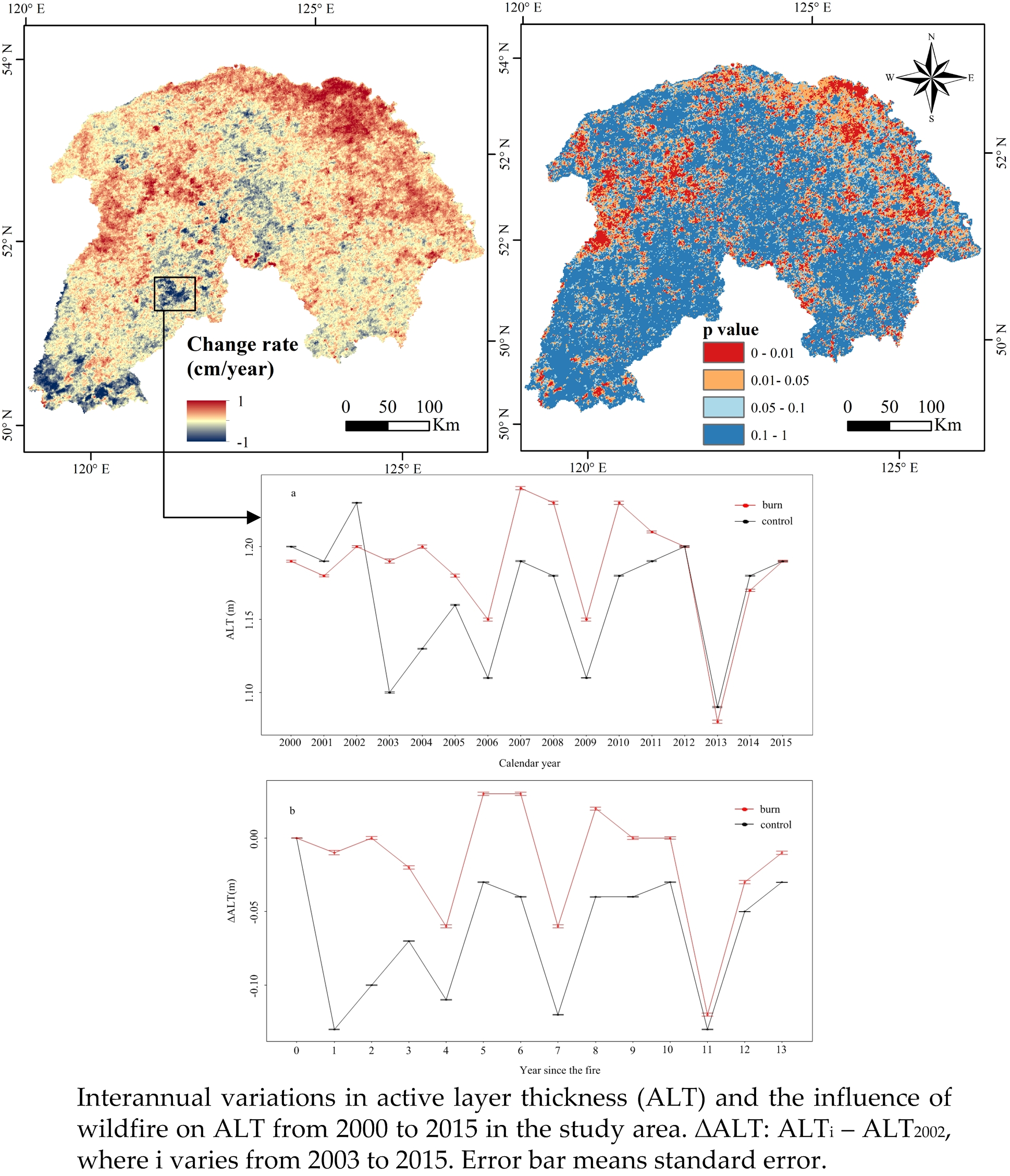
We found that GST can be robustly estimated with the MODIS LST during the thaw period (Figure 2). The relationship between LST and GST can be shown as GST = 1.0328 × LST + 0.9579 (R² = 0.71, p < 0.001). We calculated the number of degree days of thaw based on this equation and then modeled ALT using the Stefan equation. The observed and modelled mean ALT of the 13 validation sites were both 1.16 m. The mean relative error was 7%, while the root mean square error was 0.1 m, indicating an accurate representation of ALT in this study area with the Stefan equation. An increase of 50% in DDT would increase ALT by 22%, while a 50% decrease may decrease ALT by 29% (Figure 3a). Based on the data from six weather stations located in this region, the mean n-factor in the thaw period was 1.22 and its standard deviation was 0.24 over 16 years of observation, which would lead to a 10% variation in ALT (Figure 3b).

3.2. Active Layer Thickness

The mean ALT in Chinese boreal larch forests fluctuated between 1.18 and 1.3 m from 2000 to 2015 without exhibiting an obvious temporal trend. Results from the Stefan equation showed that mean ALT slightly increased in the first three years, and then decreased 0.11 m in the following seven years. After that, the mean ALT unchanged from 2010 to 2012, and then decreased by 0.08 m in 2013 while increasing 0.09 m through 2015. Interannual variations of ALT in discontinuous and sporadic permafrost areas (1.13–1.27 m and 1.22–1.33 m, respectively) were similar to the ALT of the entire study area.

Overall, ALT was low in the west-central part of the study area and high in the eastern and the southernmost parts. In most years, ALT was lower than 1.1 m in Genhe County and western Huma County, which featured the highest elevations of the study area. Active layer thickness was larger than 1.2 m in Xinlin County and eastern Huma County at relatively low elevations. The largest ALT occurred in southern Erguna County at the lowest latitude in the region. The regional-level spatial distribution pattern of ALT was similar across years of the study period.

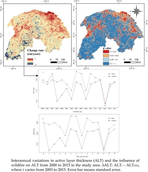
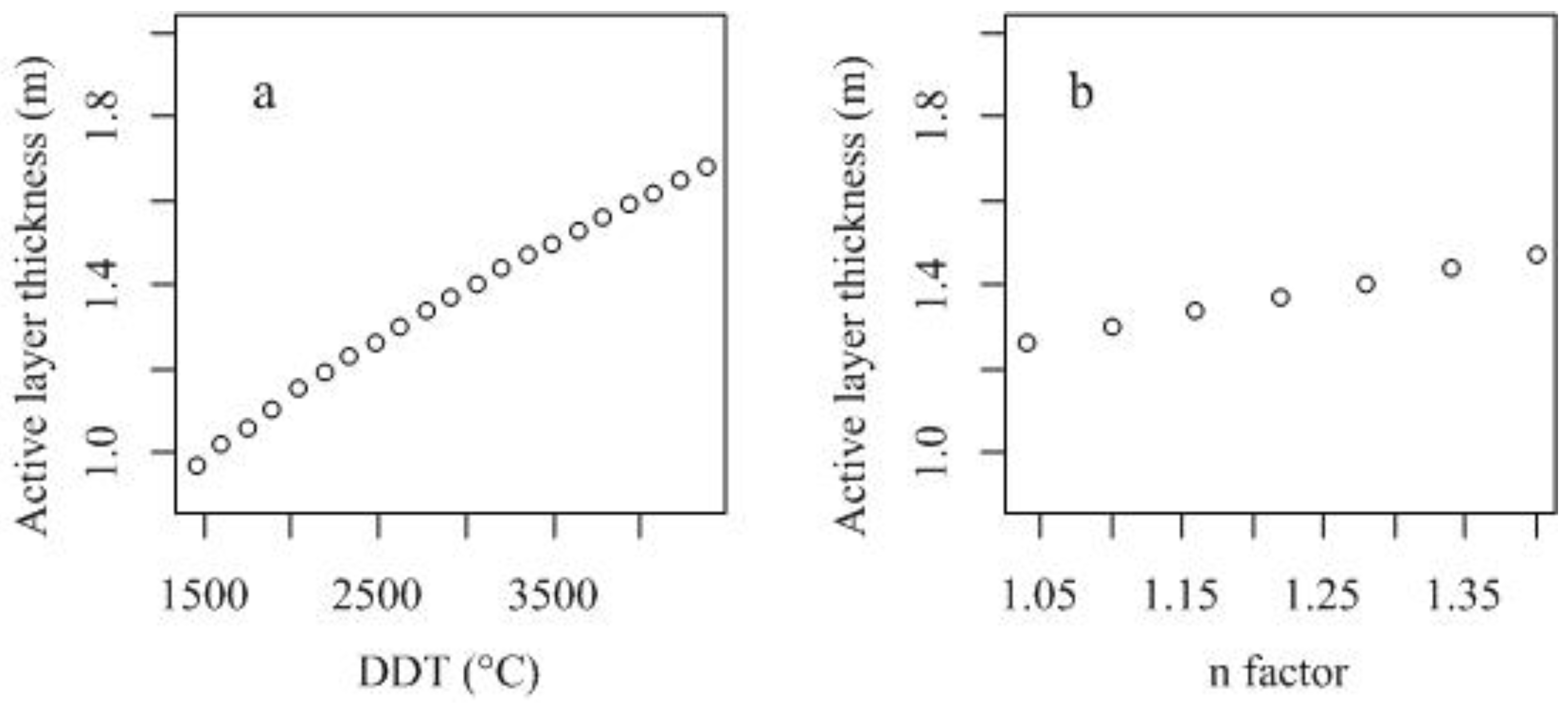
The active layer significantly deepened in northeastern Tahe, northern Mohe, eastern Huma, the center of Erguna, and the area along the border between Mohe and Genhe counties (Figure 4). Active layer depth significantly decreased in southern Erguna and some areas burned more than a decade ago. In most areas, ALT had not changed significantly. Overall, the change rate of regional-level ALT was less than 1 cm year⁻¹ (Figure 4).

3.3. Effects of Wildfire and Climatic Warming on the Active Layer

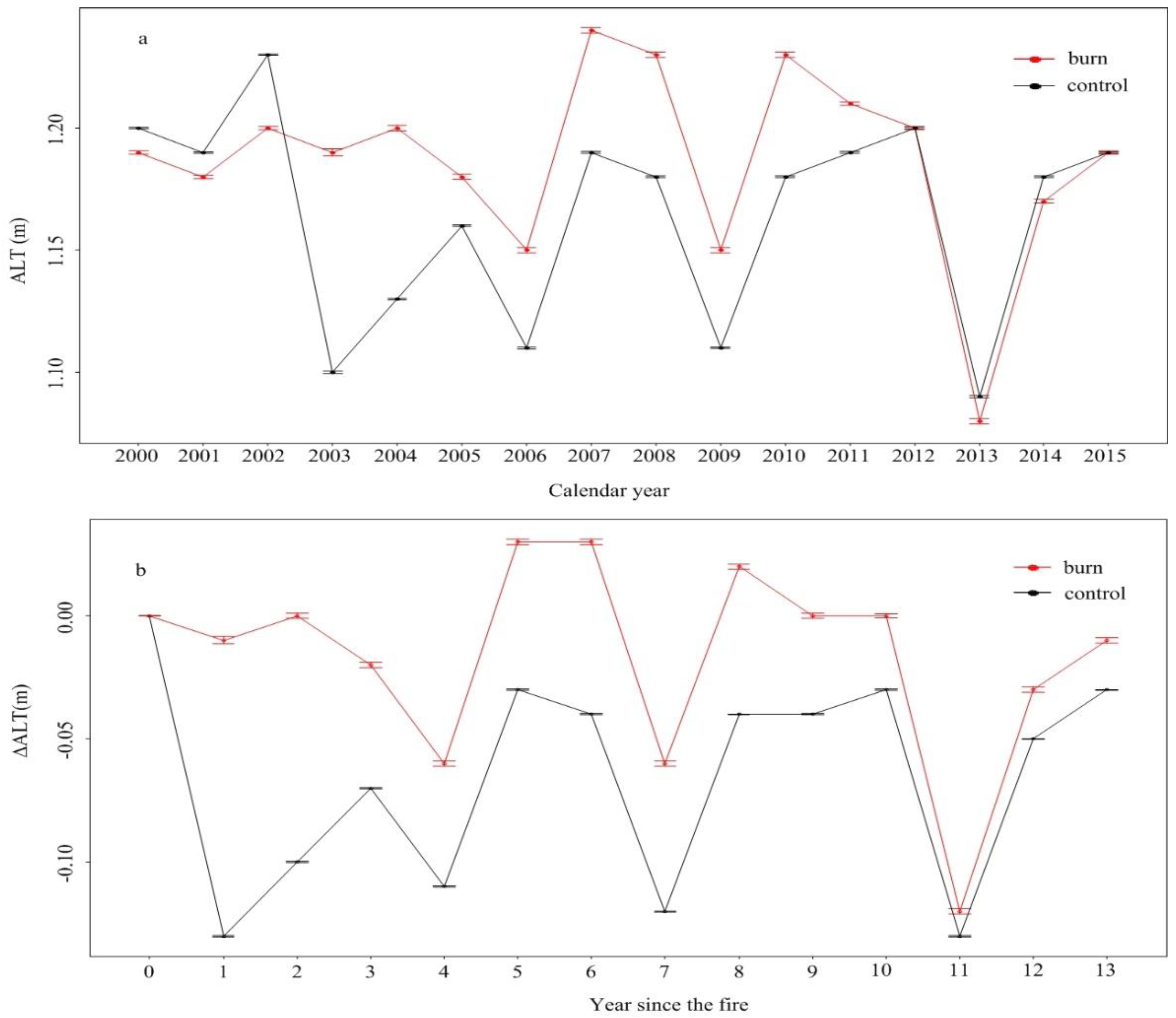
Results showed that the ALT in the burned area was greater than that in the control area from 2003 to 2012. In contrast, the ALT in the burned area was lower than in the control area before 2003 (Figure 5a). These results suggest that wildfire immediately increased the ALT with the difference in ΔALT varying significantly between the burned and control areas (p < 0.01), even though mean ΔALT in the burned area was only slightly larger than in the control area. From 2002 to 2015, ΔALT did not increase significantly in the burned area, while it increased 0.1 m in the control area (Figure 5b). In the burned area, however, ΔALT became negative in 2013. This result may imply that the effects of wildfire on ALT diminished over time, and then disappeared 10 years after the wildfire.

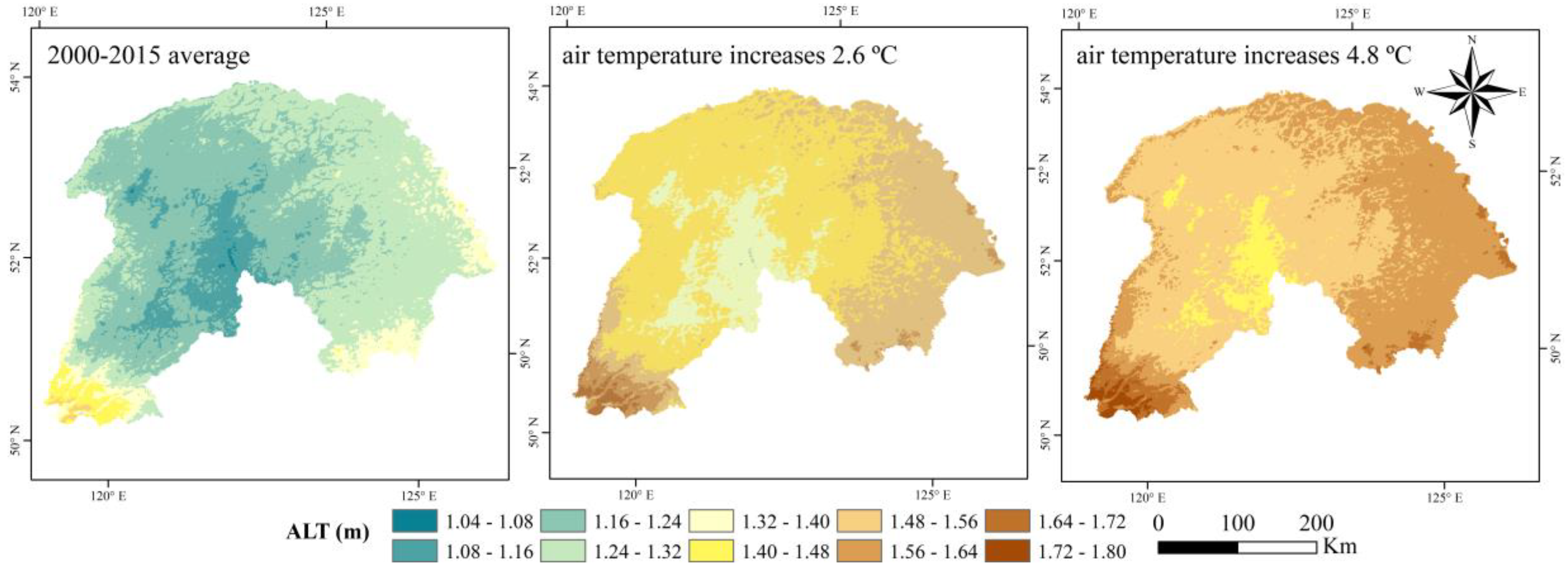
Under the RCP8.5 scenario, an increase in air temperature would increase GST by 5.22–7.69 °C, according to the regression relationship between air temperature and GST during the thaw period of the study area. Therefore, ALT would increase into 1.2–1.3 m (2.6 °C) or 1.4–1.5 m (4.8 °C) in Genhe and western Huma at high elevations. In addition, it would increase into 1.6–1.7 m (2.6 °C) or 1.7–1.8 m (4.8 °C) in the eastern and southernmost parts of the study area by 2100 where latitude and elevation are low (Figure 6). On average, ALT would increase into 1.46–1.55 m over the entire study area if the air temperature increased by 2.6–4.8 °C.

4. Discussion

4.1. Estimation of Active Layer Thickness

Our estimation results were consistent with the latitudinal temperature distribution when compared with data from Circumpolar Active Layer Monitoring program. In this program, Brown et al. [14] reported that ALT was low in northern Alaska (0.3–0.6 m) but higher in Svalbard, Norway (0.96–1.57 m). In our study area, ALT was previously measured at about 1.5–3 m by ground penetration radar near the downtown area of Mohe [47], larger than estimate in this study (1.2–1.3 m). ALT was estimated at between 1.1 and 1.2 m in Huzhong National Nature Reserve, one of the areas in western Huma. This depth was similar to the measurements from Lv et al. [48] that showed the ALT in this region was 0.4–1.4 m.

Our results differed from other studies (e.g., [25]) that suggested that permafrost was becoming degraded and the active layer had deepened as a result of global climate warming. The active layer was not only influenced by air temperature but also by topography and land cover. In comparison to estimating ALT with air temperature, LST, as the main data source of this study, provided more information on the spatial and temporal variations of the state of equilibrium at the surface [49].

4.2. Spatio-Temporal Variations in Active Layer Thickness

Although the regional-level spatial and temporal variations in ALT were largely affected by air temperature, other factors—such as vegetation, snow density and depth, slope, aspect, waterbodies, etc. [7]—also influenced the thickness and distribution of the active layer by regulating the temperature.

Mean summer air temperature increased in Mohe and Tahe counties but had no obvious trend in Xinlin and Huma counties over 16 years. Air temperature decreased in Erguna in the summer from 2011 to 2015 (Figure S3). An increase in air temperature will result in increased heat input into soil and accelerate the degradation of permafrost. Thus, the increasing trend of ALT in the northeastern part of the study area is considered to be caused by an increase in air temperature. The significant decrease of ALT in southern Erguna may have been caused by a decrease in air temperature.

Elevation was negatively correlated with ALT (p < 0.001, Figure S4) because the air temperature and GST decrease with an increase in elevation. In areas with elevations above 800 m, the mean DDT was 1898–2390 °C-day, about 261–377 °C-day lower than that in areas with elevations below 800 m. Additionally, the changes of land cover and land use will affect ALT by altering evapotranspiration and heat input into the soil. For instance, forest cover protects permafrost from degradation better than grassland because the former has a strong evapotranspiration and shading effect. Wildfire can remove the organic layers and vegetation, which will accelerate the exchange of energy between air and soil. Mean summer GST and ALT would increase after a wildfire, especially soon after a wildfire occurs. In control area of the Genhe mega-fire, the mean DDT decreased by 116–482 °C-day during 2003 to 2015 in comparison to 2002. However, the difference of DDT between pre- and post-fire was 56–423 °C-day larger in the burned area than in the control area since 2003. This result suggests that the effects of wildfire on ALT were partly offset by a decrease in DDT that presented in the control area. Vegetation restoration is expected to cause the effects of wildfire on ALT to diminish over time. Increased vegetation cover creates shading that reduces the amount of solar radiation reaching the ground and cools the surface by enhancing evapotranspiration [50]. Therefore, the change trend of ALT was negative in early burned areas. However, self-thinning becomes an active process when a young even-aged forest grows to maturity [51], resulting in a relatively open forest cover, which may increase the amount of solar radiation reaching the ground. The interannual variation of ALT is considered to be the result of the interaction between air temperature, wildfire, vegetation recovery, and self-thinning in early burned areas.

Land cover change such as building infrastructure may accelerate a deepening of the active layer. The ALT under natural surfaces is lower than under asphalt pavement because asphalt can absorb heat and reduce evaporation [52]. Logging in the study area has greatly disturbed forest environments; the present study area is one of the main sources of lumber in China. Original and secondary forests have partially disappeared because of an increase in the size of the human population in the region [25]. These anthropogenic disturbances could cause an increase in soil temperature and deepen the active layer. Brown et al. [53] found that the depth of thaw doubled after vegetation removal. Deforestation often destroys the moss and litter layers and weakens their insulating effect. This allows more insolation and wind to reach the ground surface and may increase the amount of sensible and latent heat released to the environment, especially in freezing seasons [25,54]. Human disturbance, however, has less of an effect on ALT in high elevation areas where wetlands and national nature reserves occupy a significant proportion of landscape and provide a level of environmental protection and stability.

4.3. Uncertainty Analysis

Although the Stefan equation performed well, we would like to acknowledge some uncertainties in the present study. First, we modeled ALT using 1-km MODIS data, which cannot detect the influence of microscale (<1 km) factors on ALT. Second, soil thermal conductivity was calculated by soil water content that was limited by the investigation and spatial heterogeneity. Third, the n-factor was a key parameter in the Stefan equation and impacted by soil conditions and other factors. It had spatio-temporal variability even though we analyzed parameter sensitivity. To analyze the related uncertainty, however, we found that ALT would increase about 9.5% if thermal conductivity increased by 20%; an increase of 20% in soil volumetric latent heat of fusion would result in a decrease in ALT by 8.8%. The maximum n-factor (1.48) was calculated in Tahe in 2008 while the minimum (1.09) was in Mohe in 2012. In comparison to the mean n-factor, the maximum n-factor increased ALT by 10% and the minimum decreased by 5%.

Although we modelled ALT in the future, the influence of winter air temperature and snow were not taken into account. Warming occurred in winter and spring is stronger than in summer [55], which suggests that the estimated ALT may be lower than values based on soil temperature measurements. A deep snow cover may protect soil from cold atmosphere and foster high soil moisture levels, leading to greater ALT. In contrast, some studies (e.g., [56]) indicated that snow cover had small effects on ALT. Zhang et al. [57] found that snow cover was either positively or negatively related with ALT. According to an investigation in Chinese boreal forest, snow cover with less than 15 cm has a little influence on the ground temperature, even a thickness of 15–30 cm snow thickness cannot protect ground surface temperature from the influence of the shortwave radiation reaching the snow–ground interface [58].

It is hard to predict air temperature and GST during the thaw period by 2100, resulting in uncertainty in our output. However, we used the method of replacing time with space to validate the modelled output. Mean air temperature during 2000 to 2015 was 0.15 °C in Huma and −3.59 °C in Mohe. We assumed that air temperature increased from −3.59 °C to 0.15 °C in the future, then compared GST and ALT between Huma and Mohe. Mean ALT over 16 years increased from 1.33 m to 1.43 m. Therefore, we considered that the predicted ALT by 2100 was seasonable. Using the same model, Woo et al. [59] predicted that the ALT may increase by 0.3 m by 2100 in the boreal forest of the Mackenzie Valley, which was favorably comparable with ours (increased from 1.18–1.3 m to 1.46–1.55 m).

5. Conclusions

The current research demonstrates a method for integrating modelling with remote sensing data for estimating the thickness and distribution of the active layer in Chinese boreal larch forests. Active layer thickness varied from 1.18 to 1.3 m from 2000 to 2015. Temporal variations in regional-level ALT were less than 0.1 m in most areas over 16 years, with a change trend of ±0.01 m year⁻¹. The areas of low ALT were in areas of high elevation and decreased air temperature, whereas the areas with high ALT were in areas of low elevation, nonforested land, human or natural disturbances, and increased air temperature. In the burned area of Genhe, the influence of wildfire on ALT appeared to last for 10 years. Under the high emission scenario (RCP8.5), mean ALT would increase to 1.46–1.55 m by 2100.

References

- Bonnaventure, P.P.; Lamoureux, S.F. The active layer: A conceptual review of monitoring, modelling techniques and changes in a warming climate. Prog. Phys. Geogr. 2013, 37, 352–376. [Google Scholar] [CrossRef]
- Anisimov, O.A.; Shiklomanov, N.I.; Nelson, F.E. Global warming and active-layer thickness: Results from transient general circulation models. Glob. Planet Chang. 1997, 15, 61–77. [Google Scholar] [CrossRef]
- Hinkel, K.M.; Paetzold, F.; Nelson, F.E.; Bockheim, J.G. Patterns of soil temperature and moisture in the active layer and upper permafrost at Barrow, Alaska 1993–1999. Glob. Planet Chang. 2001, 29, 293–309. [Google Scholar] [CrossRef]
- Shiklomanov, N.I.; Nelson, F.E. Analytic representation of the active layer thickness field, Kuparuk River Basin, Alaska. Ecol. Model. 1999, 123, 105–125. [Google Scholar] [CrossRef]
- Liu, L.; Schaefer, K.; Zhang, T.; Wahr, J. Estimating 1992–2000 average active layer thickness on the Alaskan North Slope from remotely sensed surface subsidence. J. Geophys. Res. Earth Surf. 2012, 117. [Google Scholar] [CrossRef]
- Romanovsky, V.E.; Osterkamp, T.E. Thawing of the active layer on the coastal plain of the Alaskan Arctic. Permafr. Periglac. Process. 1997, 8, 1–22. [Google Scholar] [CrossRef]
- Shiklomanov, N.I.; Nelson, F.E. Active-layer mapping at regional scales: A 13-year spatial time series for the Kuparuk region, north-central Alaska. Permafr. Periglac. Process. 2002, 13, 219–230. [Google Scholar] [CrossRef]
- Heggem, E.S.F.; Etzelmüller, B.; Anarmaa, S.; Sharkhuu, N.; Goulden, C.E.; Nandinsetseg, B. Spatial distribution of ground surface temperatures and active layer depths in the Hövsgöl area, northern Mongolia. Permafr. Periglac. Process. 2006, 17, 357–369. [Google Scholar] [CrossRef]
- Schuur, E.A.; Vogel, J.G.; Crummer, K.G.; Lee, H.; Sickman, J.O.; Osterkamp, T.E. The effect of permafrost thaw on old carbon release and net carbon exchange from tundra. Nature 2009, 459, 556–559. [Google Scholar] [CrossRef] [PubMed]
- Schuur, E.A.; Abbott, B. Climate change: High risk of permafrost thaw. Nature 2011, 480, 32–33. [Google Scholar] [CrossRef] [PubMed] [Green Version]
- Cannone, N.; Guglielmin, M.; Hauck, C.; Muhll, D.V. The impact of recent glacier fluctuation and human activities on permafrost distribution, Stelvio Pass (Italian Central-Eastern Alps). In Proceedings of the 8th International Conference on Permafrost, Zürich, Switzerland, 21–25 July 2003. [Google Scholar]
- Jin, H.; Yu, Q.; Wang, S.; Lü, L. Changes in permafrost environments along the Qinghai–Tibet engineering corridor induced by anthropogenic activities and climate warming. Cold Reg. Sci. Technol. 2008, 53, 317–333. [Google Scholar] [CrossRef]
- Péwé, T.L. Permafrost—And its effects on human activities in arctic and subarctic regions. GeoJournal 1979, 3, 333–344. [Google Scholar] [CrossRef]
- Brown, J.; Hinkel, K.M.; Nelson, F.E. The circumpolar active layer monitoring (calm) program: Research designs and initial results. Polar Geogr. 2000, 24, 166–258. [Google Scholar] [CrossRef]
- Hoelzle, M.; Gruber, S. Borehole and ground surface temperatures and their relationship to meteorological conditions in the Swiss Alps. In Proceedings of the Ninth International Conference on Permafrost, Fairbanks, Alaska, 25–29 June 2008. [Google Scholar]
- Beck, I.; Ludwig, R.; Bernier, M.; Lévesque, E.; Boike, J. Assessing Permafrost Degradation and Land Cover Changes (1986–2009) using Remote Sensing Data over Umiujaq, Sub-Arctic Québec. Permafr. Periglac. Process. 2015, 26, 129–141. [Google Scholar] [CrossRef] [Green Version]
- Farbrot, H.; Isaksen, K.; Etzelmüller, B.; Gisnås, K. Ground Thermal Regime and Permafrost Distribution under a Changing Climate in Northern Norway. Permafr. Periglac. Process. 2013, 24, 20–38. [Google Scholar] [CrossRef]
- Peng, X.; Frauenfeld, O.W.; Cao, B.; Wang, K.; Wang, H.; Su, H.; Huang, Z.; Yue, D.; Zhang, T. Response of changes in seasonal soil freeze/thaw state to climate change from 1950 to 2010 across china. J. Geophys. Res. Earth Surf. 2016, 121, 1984–2000. [Google Scholar] [CrossRef]
- Sazonova, T.S.; Romanovsky, V.E. A model for regional-scale estimation of temporal and spatial variability of active layer thickness and mean annual ground temperatures. Permafr. Periglac. Process. 2003, 14, 125–139. [Google Scholar] [CrossRef]
- Zhang, Y.; Olthof, I.; Fraser, R.; Wolfe, S.A. A new approach to mapping permafrost and change incorporating uncertainties in ground conditions and climate projections. Cryosphere 2014, 8, 2177–2194. [Google Scholar] [CrossRef] [Green Version]
- Leverington, D.W.; Duguay, C.R. A neural network method to determine the presence or absence of Permafrost near Mayo, Yukon Territory, Canada. Permafr. Periglac. Process. 1997, 8, 205–215. [Google Scholar] [CrossRef]
- Bartsch, A.; Kidd, R.A.; Wagner, W.; Bartalis, Z. Temporal and spatial variability of the beginning and end of daily spring freeze/thaw cycles derived from scatterometer data. Remote Sens. Environ. 2007, 106, 360–374. [Google Scholar] [CrossRef]
- Nguyen, T.N.; Burn, C.R.; King, D.J.; Smith, S.L. Estimating the extent of near-surface permafrost using remote sensing, Mackenzie Delta, Northwest Territories. Permafr. Periglac. Process. 2009, 20, 141–153. [Google Scholar] [CrossRef] [Green Version]
- Panda, S.K.; Prakash, A.; Solie, D.N.; Romanovsky, V.E.; Jorgenson, M.T. Remote sensing and field-based mapping of permafrost distribution along the Alaska Highway corridor, interior Alaska. Permafr. Periglac. Process. 2010, 21, 271–281. [Google Scholar] [CrossRef]
- Jin, H.; Yu, Q.; Lü, L.; Guo, D.; He, R.; Yu, S.; Sun, G.; Li, Y. Degradation of permafrost in the Xing’anling Mountains, northeastern China. Permafr. Periglac. Process. 2007, 18, 245–258. [Google Scholar] [CrossRef]
- Guo, D.; Li, Z. Geological evolution and age of formation of permafrost in northeastern China since the late Pleistocene. J. Glaciol. Geocryol. 1981, 3, 1–6. [Google Scholar]
- Cahoon, D.R.; Stocks, B.J.; Levine, J.S.; Cofer, W.R.; Pierson, J.M. Satellite analysis of the severe 1987 forest fires in northern China and southeastern Siberia. J. Geophys. Res. Atmos. 1994, 99, 18627–18638. [Google Scholar] [CrossRef]
- Liu, Z.; Yang, J.; Chang, Y.; Weisberg, P.J.; He, H. Spatial patterns and drivers of fire occurrence and its future trend under climate change in a boreal forest of Northeast China. Glob. Chang. Biol. 2012, 18, 2041–2056. [Google Scholar] [CrossRef]
- Cui, X.; Gao, F.; Song, J.; Sang, Y.; Sun, J.; Di, X. Changes in soil total organic carbon after an experimental fire in a cold temperate coniferous forest: A sequenced monitoring approach. Geoderma 2014, 226–227, 260–269. [Google Scholar] [CrossRef]
- Jorgenson, M.T.; Romanovsky, V.; Harden, J.; Shur, Y.; O’Donnell, J.; Schuur, E.A.G.; Kanevskiy, M.; Marchenko, S. Resilience and vulnerability of permafrost to climate change. Can. J. Earth Sci. 2010, 40, 1219–1236. [Google Scholar]
- Li, X.; Cheng, G.; Jin, H.; Kang, E.; Che, T.; Jin, R.; Wu, L.; Nan, Z.; Wang, J.; Shen, Y. Cryospheric change in China. Glob. Planet Chang. 2008, 62, 210–218. [Google Scholar] [CrossRef]
- Cai, W.; Yang, J.; Liu, Z.; Hu, Y.; Weisberg, P.J. Post-fire tree recruitment of a boreal larch forest in Northeast China. For. Ecol. Manag. 2013, 307, 20–29. [Google Scholar] [CrossRef]
- Hachem, S.; Duguay, C.R.; Allard, M. Comparison of MODIS-derived land surface temperatures with ground surface and air temperature measurements in continuous permafrost terrain. Cryosphere 2012, 6, 51–69. [Google Scholar] [CrossRef] [Green Version]
- Ran, Y.; Li, X.; Jin, R.; Guo, J. Remote Sensing of the Mean Annual Surface Temperature and Surface Frost Number for Mapping Permafrost in China. Arct. Antarct. Alp. Res. 2015, 47, 255–265. [Google Scholar] [CrossRef] [Green Version]
- Yang, Y.Z.; Cai, W.H.; Yang, J. Evaluation of MODIS Land Surface Temperature Data to Estimate Near-Surface Air Temperature in Northeast China. Remote Sens. 2017, 9, 410. [Google Scholar] [CrossRef]
- Choi, T.; Helder, D.L. Generic sensor modeling for modulation transfer function (MTF) estimation. In Proceedings of the Pecora 16 Global Priorities in Land Remote Sensing, Sioux Falls, South Dakota, 23–27 October 2005. [Google Scholar]
- Anisimov, O.A.; Shiklomanov, N.I.; Nelson, F.E. Variability of seasonal thaw depth in permafrost regions: A stochastic modeling approach. Ecol. Model. 2002, 153, 217–227. [Google Scholar] [CrossRef]
- Matyshak, G.V.; Goncharova, O.Y.; Moskalenko, N.G.; Walker, D.A.; Epstein, H.E.; Shur, Y. Contrasting Soil Thermal Regimes in the Forest-Tundra Transition Near Nadym, West Siberia, Russia. Permafr. Periglac. Process. 2015, 28, 108–118. [Google Scholar] [CrossRef] [Green Version]
- Smith, M.W.; Riseborough, D.W. Permafrost monitoring and detection of climate change. Permafr. Periglac. Process. 1996, 7, 301–309. [Google Scholar] [CrossRef]
- Smith, S.L.; Riseborough, D.W.; Bonnaventure, P.P. Eighteen Year Record of Forest Fire Effects on Ground Thermal Regimes and Permafrost in the Central Mackenzie Valley, NWT, Canada. Permafr. Periglac. Process. 2015, 26, 289–303. [Google Scholar] [CrossRef]
- Kersten, M.S. Laboratory Research for the Determination of Thermal Properties of Soils; ACFEL Tech Rep 23; University of Minnesota: Minneapolis, MN, USA, 1949. [Google Scholar]
- Zhang, Y.; Sun, M.; Liu, T. Effect of Forest Fire on Soil Physical and Chemical Properties of typical Forests in Daxing’an Mountains. J. Northeast For. Univ. 2012, 40, 41–43. (In Chinese) [Google Scholar]
- Wilhelm, K.R.; Bockheim, J.G.; Kung, S. Active Layer Thickness Prediction on the Western Antarctic Peninsula. Permafr. Periglac. Process. 2015, 26, 188–199. [Google Scholar] [CrossRef]
- IPCC. Climate Change 2014: Synthesis Report. Contribution of Working Groups I, II and III to the Fifth Assessment Report of the Intergovernmental Panel on Climate Change; Core Writing Team, Pachauri, R.K., Meyer, L.A., Eds.; IPCC: Geneva, Switzerland, 2014; p. 151. [Google Scholar]
- Hamby, D.M. A review of techniques for parameter sensitivity analysis of environmental models. Environ. Monit. Assess. 1994, 32, 135–154. [Google Scholar] [CrossRef] [PubMed] [Green Version]
- Dilts, T.E.; Yang, J.; Weisberg, P.J. The landscape similarity toolbox: New tools for optimizing the location of control sites in experimental studies. Ecography 2010, 33, 1097–1101. [Google Scholar] [CrossRef]
- Chen, L.; Yu, W.; Yi, X.; Wu, Y.; Ma, Y. Application of ground penetration radar to permafrost survey in Mohe County, Heilongjiang Province. J. Glaciol. Geocryol. 2015, 37, 723–730. [Google Scholar]
- Lv, J.; Li, X.; Hu, Y.; Wang, X.; Liu, H.; Bing, L. Factors affecting the thickness of permafrost’s active layer in Huzhong National Nature Reserve. Chin. J. Ecol. 2007, 26, 1369–1374. [Google Scholar]
- Li, Z.; Tang, B.; Wu, H.; Ren, H.; Yan, G.; Wan, Z.; Trigo, I.F.; Sobrino, J.A. Satellite-derived land surface temperature: Current status and perspectives. Remote Sens. Environ. 2013, 131, 14–37. [Google Scholar] [CrossRef] [Green Version]
- Zhou, L.; Dickinson, R.E.; Tian, Y.; Vose, R.S.; Dai, Y. Impact of vegetation removal and soil aridation on diurnal temperature range in a semiarid region: Application to the Sahel. Proc. Natl. Acad. Sci. USA 2007, 104, 17937–17942. [Google Scholar] [CrossRef] [PubMed] [Green Version]
- Aguirre, A.; del Río, M.; Condés, S. Intra-and inter-specific variation of the maximum size-density relationship along an aridity gradient in Iberian pinewoods. For. Ecol. Manag. 2018, 411, 90–100. [Google Scholar] [CrossRef]
- Wu, Q.; Shi, B.; Fang, H. Engineering geological characteristics and processes of permafrost along the Qinghai–Xizang (Tibet) Highway. Eng. Geol. 2003, 68, 387–396. [Google Scholar] [CrossRef]
- Brown, J.; Rickard, W.; Vietor, D. The effect of disturbance on permafrost terrain. Cold Reg. Res. Eng. Lab. Spec. Rep. 1969, 138, 1–13. [Google Scholar]
- Zhang, T.; Osterkamp, T.E.; Stamnes, K. Effects of Climate on the Active Layer and Permafrost on the North Slope of Alaska, U.S.A. Permafr. Periglac. Process. 1997, 8, 45–67. [Google Scholar] [CrossRef]
- Serreze, M.C.; Walsh, J.E.; Iii, F.S.C.; Osterkamp, T.; Dyurgerov, M.; Romanovsky, V.; Oechel, W.C.; Morison, J.; Zhang, T.; Barry, R.G. Observational Evidence of Recent Change in the Northern High-Latitude Environment. Clim. Chang. 2000, 46, 159–207. [Google Scholar] [CrossRef]
- Ling, F.; Zhang, T. Impact of the timing and duration of seasonal snow cover on the active layer and permafrost in the Alaskan Arctic. Permafr. Periglaci. Process. 2003, 14, 141–150. [Google Scholar] [CrossRef]
- Zhang, T.J.; Frauenfeld, O.W.; Serreze, M.C.; Etringer, A.; Oelke, C.; McCreight, J.; Barry, R.G.; Gilichinsky, D.; Yang, D.Q.; Ye, H.C.; et al. Spatial and temporal variability in active layer thickness over the Russian Arctic drainage basin. J. Geophys. Res. 2005, 110, 110. [Google Scholar] [CrossRef]
- Chang, X.; Jin, H.; Zhang, Y.; He, R.; Luo, D.; Wang, Y.; Lü, L.; Zhang, Q. Thermal Impacts of Boreal Forest Vegetation on Active Layer and Permafrost Soils in Northern da Xing’Anling (Hinggan) Mountains, Northeast China. Arct. Antarc. Alp. Res. 2015, 47, 267–279. [Google Scholar] [CrossRef]
- Woo, M.; Mollinga, M.; Smith, S.L. Climate warming and active layer thaw in the boreal and tundra environments of the Mackenzie Valley. Can. J. Earth Sci. 2007, 44, 733–743. [Google Scholar] [CrossRef]
Figure 1.
The geographic location of the study area showing county boundaries of the Inner Mongolia Autonomous Region (Erguna and Genhe) and Heilongjiang Province within the study area; the area of discontinuous permafrost; and locations of a mega-fire, validation points, and meteorological stations. An inset map shows the location of the study area within China. The study area is covered by discontinuous (pink area) and sporadic permafrost (outside of pink polygon).
Figure 2.
Regression analysis of the linear relationship between ground surface temperature (GST) and land surface temperature (LST) during the thaw period. The red and black lines show 1:1 ratio and the regression line, respectively.
Figure 3.
Active layer thickness in response to the sensitivity of parameters of (a) the degree-day of thaw (DDT) and (b) summer n-factor in the Stefan equation.
Figure 4.
The Mann–Kendall Sen’s slope of the four-year moving averaged active layer thickness (m year−1) and the corresponding confidences (p values) of the change trend from 2000 to 2015 in the study area.
Figure 5.
Interannual variations in (a) active layer thickness (ALT) and (b) ∆ALT (ALTi – ALT2002, where i varies from 2003 to 2015) in burned and control areas in Genhe County. Error bar means standard error.
Figure 6.
Active layer thickness (ALT) under the high-emission scenario RCP8.5 by 2100.
© 2018 by the authors. Licensee MDPI, Basel, Switzerland. This article is an open access article distributed under the terms and conditions of the Creative Commons Attribution (CC BY) license (http://creativecommons.org/licenses/by/4.0/).
Share and Cite
MDPI and ACS Style
Bai, X.; Yang, J.; Tao, B.; Ren, W. Spatio-Temporal Variations of Soil Active Layer Thickness in Chinese Boreal Forests from 2000 to 2015. Remote Sens. 2018, 10, 1225. https://doi.org/10.3390/rs10081225
AMA Style
Bai X, Yang J, Tao B, Ren W. Spatio-Temporal Variations of Soil Active Layer Thickness in Chinese Boreal Forests from 2000 to 2015. Remote Sensing. 2018; 10(8):1225. https://doi.org/10.3390/rs10081225
Chicago/Turabian StyleBai, Xiongxiong, Jian Yang, Bo Tao, and Wei Ren. 2018. "Spatio-Temporal Variations of Soil Active Layer Thickness in Chinese Boreal Forests from 2000 to 2015" Remote Sensing 10, no. 8: 1225. https://doi.org/10.3390/rs10081225
Note that from the first issue of 2016, this journal uses article numbers instead of page numbers. See further details here.