Long Time Behavior and Global Dynamics of Simplified Von Karman Plate Without Rotational Inertia Driven by White Noise

1
Division of Dynamics and Control, School of Astronautics, Harbin Institute of Technology, Harbin 150001, China
2
Division of Dynamics and Control, School of Mathematics and Statistics, Shandong University of Technology, Zibo 255000, China
3
School of Mathematics, Southwest Jiaotong University, Chengdu 610031, China
*
Authors to whom correspondence should be addressed.
Symmetry 2018, 10(8), 315; https://doi.org/10.3390/sym10080315
Submission received: 5 June 2018
/
Revised: 20 July 2018
/
Accepted: 22 July 2018
/
Published: 1 August 2018
(This article belongs to the Special Issue New Trends in Dynamics)
Abstract
:Without the assumption that the coefficient of weak damping is large enough, the existence of the global random attractors for simplified Von Karman plate without rotational inertia driven by either additive white noise or multiplicative white noise are proved. Instead of the classical splitting method, the techniques to verify the asymptotic compactness rely on stabilization estimation of the system. Furthermore, a clear relationship between in-plane components of the external force that act on the edge of the plate and the expectation of radius of the global random attractors can be obtained from the theoretical results. Based on the relationship between global random attractor and random probability invariant measure, the global dynamics of the plates are analyzed numerically. With increasing the in-plane components of the external force that act on the edge of the plate, global -bifurcation, secondary global -bifurcation and complex local dynamical behavior occur in motion of the system. Moreover, increasing the intensity of white noise leads to the dynamical behavior becoming simple. The results on global dynamics reveal that random snap-through which seems to be a complex dynamics intuitively is essentially a simple dynamical behavior.
1. Introduction
1.1. Background and Literatures Review
There exists an essential difference between full Von Karman plate without rotational inertia and simplified Von Karman plate without rotational inertia. From the view of physics, the former takes account into the acceleration in-plane and the latter neglects it [1,2]. In the mathematical standpoint, the governing equations of full Von Karman plates without rotational inertia comprise coupled plate equations and wave equations, while the coupled plate equation and elliptic equation compose the governing equations of Von Karman plate [3].
The definition of global random attractors for random dynamical system (RDS) established by Arnold [4] were proposed by Crauel and Flandoli [5] and Schmalfuss [6]. The former developed the theory of global random attractors in phase space, while the random attractor is seen as a subset in the space of probability measures by Schmalfuss. Afterwards, Crauel et al. [7] introduced a notion of global random attractors which is accessible to the researcher who are not familiar to the probabilistic language. Furthermore, the assertion that global random attractors are uniquely determined by attracting deterministic compact sets in phase space was attained by Crauel in [8]. Invoking these theories, the existence of global random attractors for RDS related to a plenty of mathematical physics problems have been studied by many researchers, (e.g., [9,10,11,12,13,14] and the references therein).
Von Karman plate equation is a well-known model that arise in nonlinear elastodynamics, which can be found in many engineering applications, for instance, wing skin in airplane, vertical fins of High-speed aircraft, etc. For more details, see the Introduction in Monograph [1]. There is an abundant achievements on Von Karman plate and the brief list given below is by no means exhaustive. Invoking the adjoint method, Pappalardo and Guida [15] considered the optimal control problem associated with the vibration of Von Karman plates. Utilizing the theory of plate theory, monohull ship was modelled by Fortuna and Muscato [16]; moreover, the problem of identification and adaptive control were also investigated. To compute the modal parameters of the plates, the system identification algorithm was proposed by Pappalardo and Guida [17]. A survey on computational methods for motion of multibody systems (include plates) was made by Pappalardo and Guida [18]. For the sake of computing the motion of large deformation of the plates, Pappalardo et al. [19,20,21] developed different kinds of plate/shell finite elements.
From the mathematical view, to address the long time behavior of the mathematical physics problems, it must be verified that they can generate a dynamical system, which can be accomplished by achieving the existence and uniqueness of the solution for the systems. Lasiecka [22] was concerned with weak, classical and intermediate solutions to full von Karman equations. With respect to the nonautonomous case, one can refer to Leiva and Sivoli [23] and Abels et al. [24]. According to the proof of a “sharp regularity” estimates of the Von Karman bracket, the consequence of global existence, uniqueness and regularity of solutions for simplified Von Karman plate with nonlinear boundary dissipation can be founded in Favini et al. [25]. For more detail, one can refer to the Monograph [26]. As for the long time behavior of the Von Karman plate equations, the global attractors as well as inertial manifolds for the system in autonomous situation were studied by Chueshov and Lasiecka [27] and Chueshov and Lasiecka [28], respectively. Lasiecka [29] studied the uniform decay rates for thermoelastic full von karman system. Dynamics of a thermoelastic von Karman plate in a subsonic gas flow was addressed by Ryzhkova [30]. For a von Karman plate equation with a boundary memory condition which can even be a fractional damping, Park and Sun [31] tackled the uniform decay of the solution. For more detail of the research status of long time behavior of the Von Karman plate before the year 2010, one can refer to Monograph [26]. The study of long-time dynamics of a von Karman equation with time delay is due to Park [32]. Chueshov [33] investigated questions related to global attractors for delayed, nonrotational von Karman plates without any damping in the status of flow–structure interactions. Eliminating flutter for clamped von Karman plates in subsonic flows was concerned by Lasiecka and Webster [34]. Without assuming large values for the coefficient of damping, Khanmamedov [35] proved the existence of the global random attractors for Von Karman plate equation. With a very strict assumption on the coefficient of the weakly damping, the existence of global random attractors for simplified Von Karman plate without rotational inertia driven by multiplicative white noise was studied by Chen et al. [36].
The study on dynamics of Von Karman plates can be divided into two parts: the investigation of local dynamics and investigation of global dynamics. There exists abundant studies on local dynamics for Von Karman plates. For instance, invoking the Bubnov–Galerkin approach, Awrejcewicz and Krysko [37] analyzed the complex parametric vibrations of plates and shells. Nonlinear vibration and dynamic response as well as Thermal post-buckling of functionally graded thermoelastic Von Karman plates was considered by Huang and Shen [38] and Park and Kim [39], respectively. Employing the Homotopy perturbation technique, Rashidi et al. [40] studied the nonlinear vibration of Von Karman rectangular plate. Ghayesh et al. [41] tackled the nonlinear dynamics of axially moving Von Karmam plates. Ghayesh and Farokhi [42] were devoted to handling the nonlinear dynamics of Von Karman plate in MEMS. The nonlinear vibrations of viscoelastic Von Karman plate was analyzed by Amabili [43]. The global dynamics of nonlinear systems which can reveal more dynamic information than local dynamics are important in engineering applications. Compared with the literature on local dynamics, the investigation related to global dynamics is insufficient. Global dynamics of four-dimensional perturbed Hamiltonian systems and parametrically forced mechanical systems were addressed by Wiggins [44] and Feng and Wiggins [45], respectively. The technique employed in those works is Melnikov method which was invoked by Zhang to tackle a parametrically Von Karman plate in [46]. Due to the lack of analytical tools, numerical method is the main approach to study the global dynamics of nonlinear systems. According to Cell to Cell mapping method proposed by Hsu [47], Xu et al. [48] addressed global stochastic bifurcation in Duffing system.
There exist two standpoints in study on dynamics of random dynamical system, which are equivalent in the deterministic case, the “static” standpoint and the “dynamical” standpoint. However, two views are very different in the stochastic status (see [4,49,50]). The investigation on dynamics of the RDS associated with vibration of Von Karman plates in this paper means study the of “dynamical” dynamics of the systems; alternatively, the global dynamics in this paper are understood as the change in the pattern of existing probability invariant measures of the RDS. There exist some results on global dynamics on RDS. Crauel and Flandoli [49] asserted that additive noise destroys pitchfork bifurcation in one dimensional system. The statement that parametric noise (even a multiplicative white noise) destroys Hopf bifurcation was duo to Arnold et al. [51]. Wang [52] focused on the bifurcation for stochastic parabolic equations. The investigation on stochastic bifurcation in Duffing system by the theory of random attractors was due to Schenk-Hoppé [53]. According to some invariant manifolds to derive the lower bounds on the dimension of global random attractors, Caraballo et al. [54] studied the stochastic pitchfork bifurcation of the reaction diffusion equation with multiplicative white noise.
1.2. Formulation and Contribution of This Investigation
In some circumstances, the Von Karman plate equation that epitomizes certain distinct features and mathematical difficulties which lead to the “splitting method” [55], a traditional approach in the study on the existence of global random attractors, for extensive mathematical problems becomes invalid, such as SAVKP and SMVKP (introduced in Section 2.1). The existence of global attractors for the system in deterministic case (such as Chueshov and Lasiecka [27]) and stochastic case (e.g., [36]) relies on large enough value of damping coefficient. To our best knowledge, there hardly exists results on global random attractors for SAVKP and SMVKP with arbitrary small coefficient of the weakly damping.
Recently, the study on dynamics of Von Karman plate equation mainly focused on the local dynamics, inspired by Crauel [49] and Schenk-Hoppé [53]. Based on the existence of global random attractors and the relationship between invariant measure and global random attractor summarized in Proposition 2 in Section 3.1, the dynamics of Von Karman plate can be accomplished by employing the stochastic subdivision algorithm method proposed by Keller and Ochs [56] to achieve the global random attractors numerically.
As far as we know, the consequence of investigation in this aspect also do not be published in any composition. The purpose of this paper is to investigate the existence of global random attractors for SAVKP and SMVKP and to derive the global dynamics by achieving the structure of their global random attractors.
1.3. Organization of the Paper
The rest of this paper is organized as follows. In Section 2, the mathematical description of model and main results main results are given. Section 3 is intended to provided preliminary results employed in accomplishing the main proof which are given in Section 4. Finally, based on the main results listed in Section 3, summary and conclusions is made in Section 5.
Finally, to express the results and their respective proofs succinctly, the following conventions are made. Unless otherwise stated, in the sequel, the letter , are positive constants; in addition, and , , are positive constants depended on .
2. The Mathematical Model and Main Results
Section 2.1 is used to make the mathematical description of the model considered in this paper. The main results of this paper are listed in Section 2.2.
2.1. Mathematical Description of the Model
Let be a bounded domain with boundary ; without loss of generality, assume the origin 0 belongs to . Suppose is an arbitrarily given point, while denotes the arc, oriented in the usual manner, joining the origin 0 to the point along the boundary of D. For more details, one can refer to Ciarlet [3]. The governing equation of simplified Von Karman plate without rotational inertia is:
with the clamped boundary
where U is transversal displacement of the plate. is Von Karman bracket [26] (also known as Monge-Ampère form [3]) with the form of
is the Airy function satisfies
in which the physical parameter can refer to [1]. is defined as
and
where are components of the in-plane force on boundary along the direction , which comply with
where are membrane forces in the plate; for more details, one can refer to [3]. Moreover, let , be the solution of the following system
satisfies
Thus, Equation (1) can be rewritten as:
In some cases, only is named Airy function, while is called the in-plane force, (see Chueshov and Lasiecka [26]). This convention is employed in this paper.
To formulate the system tackled in this paper, some spaces are introduced in the following. Let ,,,, where , , are the usual Sobolev Spaces. Let , then A is self-adjoint, positive, unbounded linear operators and is compact. Therefore, their eigenvalues satisfy and the corresponding eigenvalues forms an orthonormal basis in . Then, we can interpret the power of by the method developed by Temam [55]. Specifically, , however, it is mentioned here that . Nevertheless, it is emphasized here that with the boundary in Equation (2). In fact, the operator with the boundary condition in Equation (2) is a self-adjoint, positive, unbounded linear operators from to and is compact. Thus, the power of can be defined; furthermore, .
Suppose P is a stochastic pressure signified by white noise, then the dynamics equation of abstract dimensionless clamped simplified Von Karman plate without rotational inertia driven by white noise are as follow
with the clamped boundary condition
where is the dimensionless transversal displacement of the plate. are a given constant,
W is the one dimensional two-sided real-valued standard Wiener process, and is called white noise. is the coefficient of damping.
Equation (10a) describes abstract dimensionless clamped simplified Von Karman plate without rotational inertia driven by additive/multiplicative white noise, respectively. Furthermore, satisfies
and is in agreement with
where are derived from Equations (3) and (4). By the monograph of Lions and Magenes [57], , define
The system described by Equations (10a), (10c), and (10e)–(10h) is denoted by SAVKP. The system interpreted by Equations (10b), (10c), and (10e)–(10h) is represented by SMVKP.
Invoking the compactness of A, the Hilbert space with norm and can be defined as the mechanism in Temam [55], especially, . Moreover, for all , can be compact imbedding in and the following holds
Let equipped with Graph norm and the induced inner product, then they are all Hilbert spaces.
Let be a separable space with Borel algebra and be a probability space. is a family of measure preserving transformations such that is measurable, for all . Then, the flow together with the probability space is called a metric dynamical system. For the particular applications in this paper, the metric dynamical systems generated by a one dimensional two-sided standard Wiener process defined on a Probability space is introduced there. Let , is the algebra induced by the compact open topology for this set and is the Wiener measure on . Set
according to Arnold [4], we have is ergodic with respect to the flow . Thus, is the metric dynamical systems employed in this paper. Moreover, the Ornstein–Uhlenbeck process, which should be used in transforming a stochastic system to a random system, is introduced as follows
in which . The general form for the solution of Equation (13) is
Let
where is defined by Equation (12) in Section 2. Merging with integration by parts, is the solution for the system in Equation (13).
Although by no means always, it will be convenient to reduce Equations (10a) and (10b) to an evolution equation of the first order in time in the following manner. Let , then Equation (10a) can be transformed to the ensuing form
where
and
The system described by Equations (10c), (15) and (10e)–(10h) denoted by SAVKPT1. Obviously, SAVKP is equivalent to SAVKPT1.
To accomplish the stabilization estimation for the solution of SAVKPT1, the following systems is needed. Suppose are two solution of SAVKPT1, then
where .
Furthermore, let and
thus
where
here
Equation (18) is a partial differential equations with random coefficient which can be studied by . Let SAVKPT2 signify the system described by Equations (18), (10c) and (10e)–(10h). It is emphasized that SAVKPT2 is not equivalent to SAVKPT1.
Analogously, let and
define , the following system associated with SMVKP can be attained.
in which
and
where
SMVKPT1 represents the systems defined by Equations (20), (10c) and (10e)–(10f), then SMVKP and SMVKPT1 are equivalent. The system described by Equations (21), (10c) and (10e)–(10f) is denoted by SMVKPT2.
Furthermore, assume are two solutions of SAVKPT2, thus
in which
Equation (22) is used to obtain the stabilization estimation for SMVKPT1.
Remark 1.
For the sake of brevity, when no ambiguity is possible, the symbols used in SAVKPT and SMVKPT, SAVKPT1 and SMVKPT1, and SAVKPT2 and SMVKPT2 are the same or similar. Since each of the symbols has a clearl explanation, it is not confusing to express the main results in this paper. However, it must be kept in mind that they are not the same.
2.2. Main Results
Approved by the equivalent between SAVKPT and SAVKPT1, and SMVKPT and SMVKPT1, it is enough to only address the dynamical behavior of SAVKPT1 and SMVKPT1. This subsection is used to present the main results of this paper. Let
2.2.1. Random Attractors in Additive White Noise Case
This part is devoted to providing the main results for SAVKPT1. The following Theorem considers the existence and uniqueness of solution for SAVKPT2.
Theorem 1.
For any given initial value , there exists a uniqueness (mild) solution for SAVKPT2
Furthermore, let , which means that is the solution mapping of SAVKPT2. Then,
Let
by means of Theorem 1, is the RDS induced by SAVKPT2. Correspondingly, SAVKPT1 can also generate a RDS which is defined as
here is defined by Equation (17). Furthermore, the solution mapping determined by SAVKPT1 is denoted by , then
The following turns to the existence of global random attractors for SAVKPT1.
Let be any given positive constant, and
in which
are constants that satisfy Equation (45) in Section 3.2.1.
The next theorem considers the existence and expectation of radius of global random attractors for .
Theorem 2.
possesses the global random attractors in which satisfies -a.s.
where denotes the open ball centered at the origin with radius is , while M is given by Equation (A24) in Section 3.2.1.
2.2.2. Random Attractors in Multiplicative White Noise Case
The main results for SMVKPT1 is given in this part.
The form of following theorem is very similar to the Theorem 1.
Theorem 3.
For any given initial value , SMVKPT2 possesses uniqueness (mild) solution .
Furthermore, set , which indicates that is the solution mapping of SMVKPT2. Thus,
Therefore, set
then, the RDS induced by SMVKPT2 and RDS defined as follow
is the RDS generate by SMVKPT1, where is defined by Equation (19). In additive, let
Thus, is the solution mapping of SMVKPT1.
The following turns to the existence of global random attractors for SMVKPT1.
Suppose is any given positive constant, and
Set
where are constants satisfying Equation (45) in Section 3.2.2. Then, the existence and finite expectation of radius of global random attractors for can be asserted by the next theorem.
Theorem 4.
There exists global random attractors for in ; moreover,
where denotes the open ball centered at the origin with radius is , while M is given by Equation (A43) in Section 3.2.2.
Comparing Theorems 1 and 3, as well as Theorems 2 and 4, their forms are the same or similar, while there exists essential difference between them, which is expounded in Section 5.
2.2.3. Global Dynamics in Both Additive and Multiplicative White Noise Cases
Based on the theoretical results and the relationship between invariant measures and global attractors introduced in Proposition 2 in Section 3.1, the rest of this subsection is dedicated to studying the global dynamics of the stochastic Von Kaman plates, which is accomplished by deriving the components of global random attractor numerically, the main components are referred as global random point attractor and global random basic attractor. The modal equations associated with the stochastic Von Karman plates which are not display here (see Equation (A1) in Appendix A) can be obtained by employing inertial manifold with delay [58] and nonlinear gakerlin method [59].
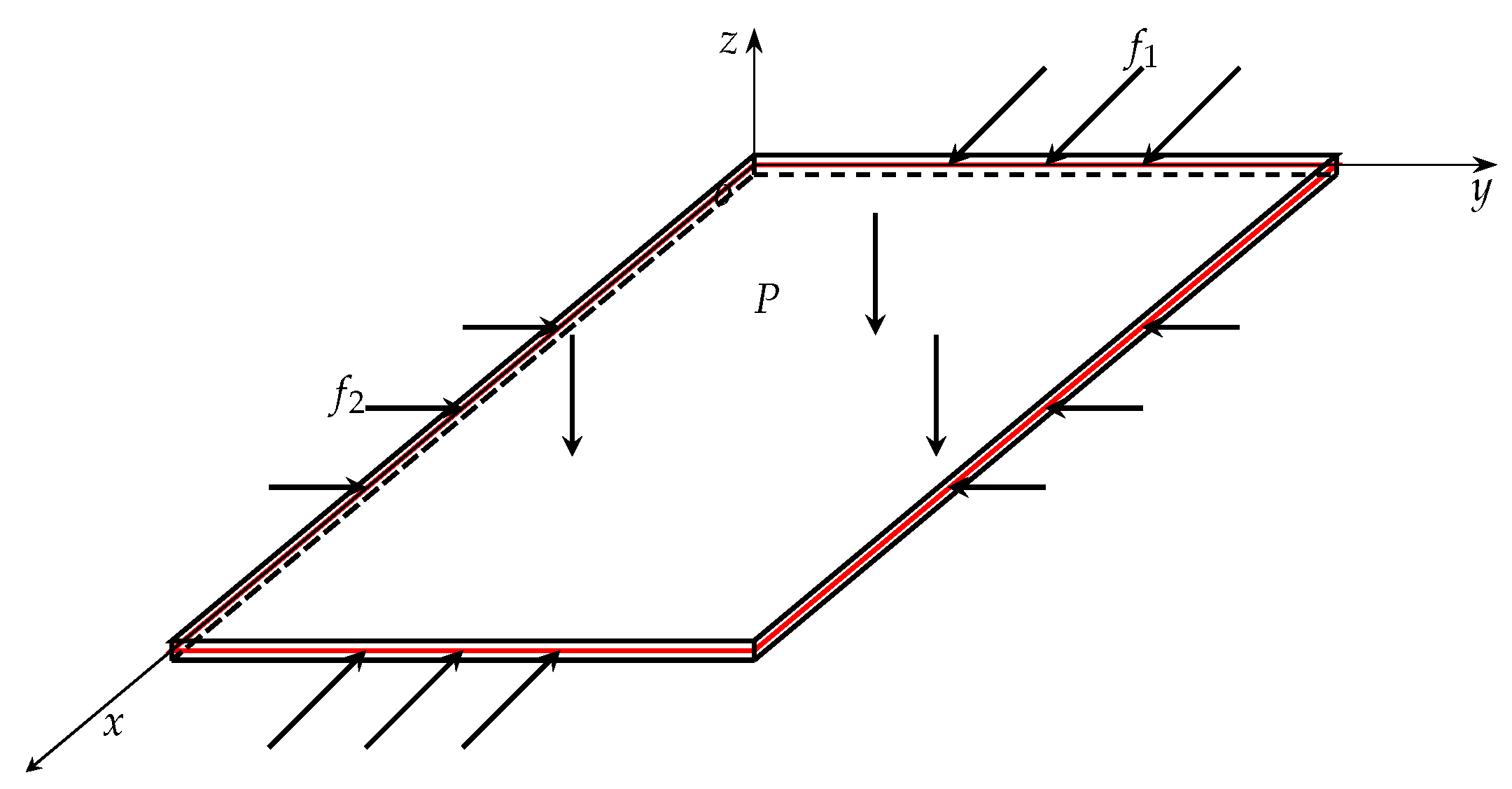
Let , in Appendix A, Figure 1 shows the model for vibration of Von Karman plate. The eigenvalues and eigenvectors of operator A and integration with respect to space variable in Equation (A2) listed in Appendix A can be performed by COMSOL with Matlab [60], and then the solution of model equations can be obtained by stochastic Runge–Kutta method [61].
The situation of additive white noise. In this case, the P in Figure 1 is equal to , let , , and are component of the in-plane force on boundary along the direction , thus the in Equation (10h) can be derived by Equations (3) and (4). Since D is rectangle, . Furthermore, let , the dynamics of simplified Von Karman plate without rotational inertia driven by additive white noise is signified by the motion of the position of the plate, which are studied in the following cases.
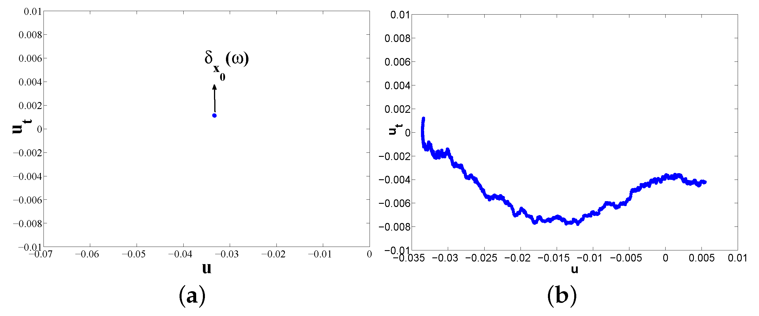
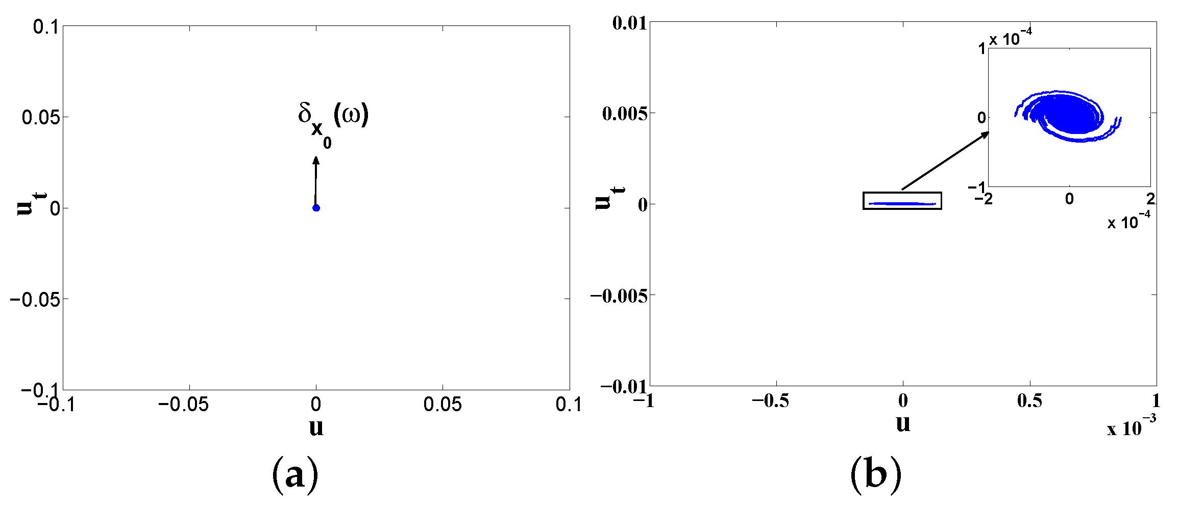
Case I. Let ,; the global random basic attractor, global random point attractor and global random attractors for SAVKP are the same. Figure 2 shows that global random basic attractor is a random fixed point which supports a invariant Markov measure . Furthermore, is almost surely global stability.
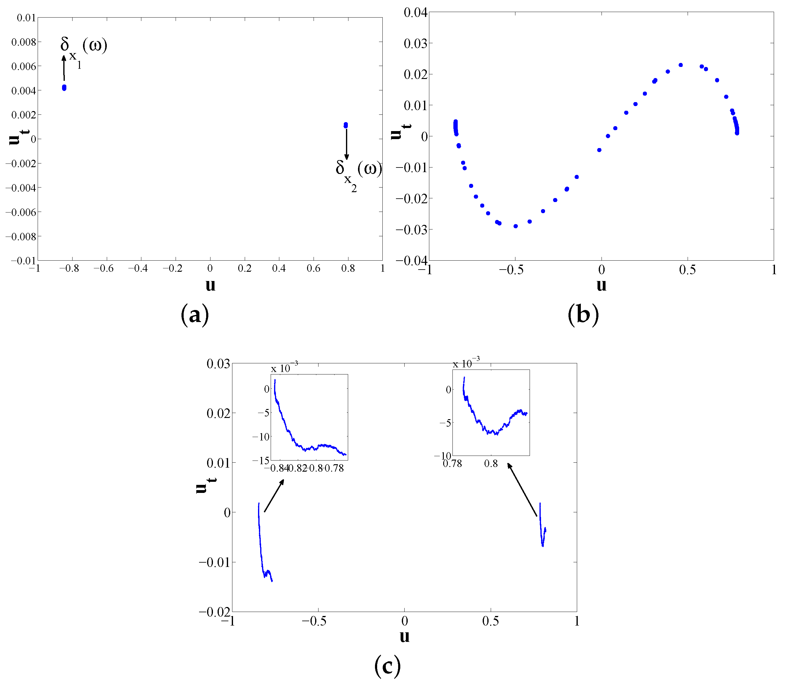
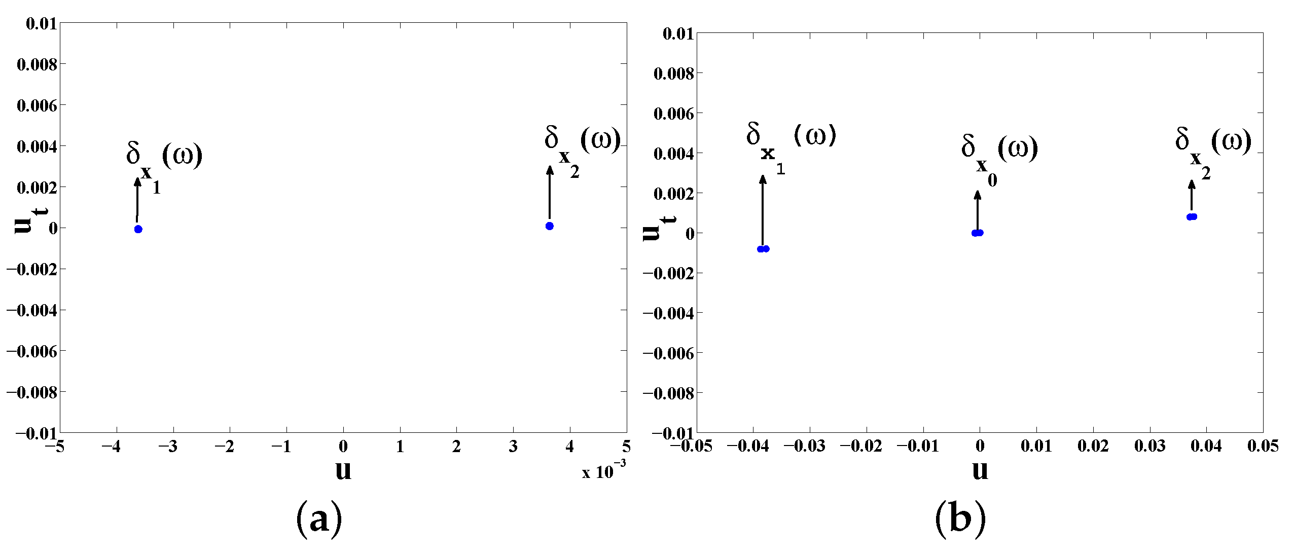
Case II. Set , in this situation, global random basic attractor is equivalent to global random point attractor. Global random basic attractor (see Figure 3c) and its section (see Figure 3a) indicate that the system possesses two invariant Markov measures which are supported by two fixed random points. Figure 3b illustrates the section of the global random attractor of SAVKP.
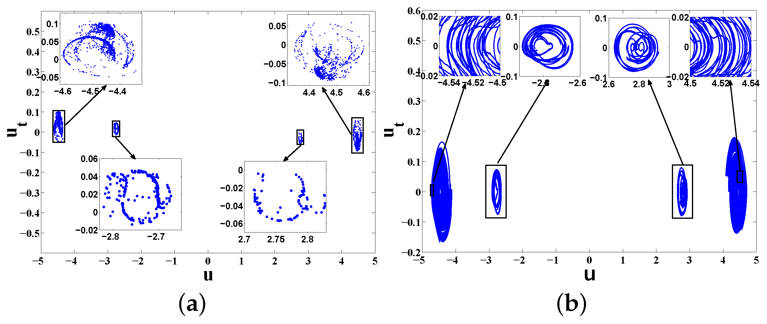
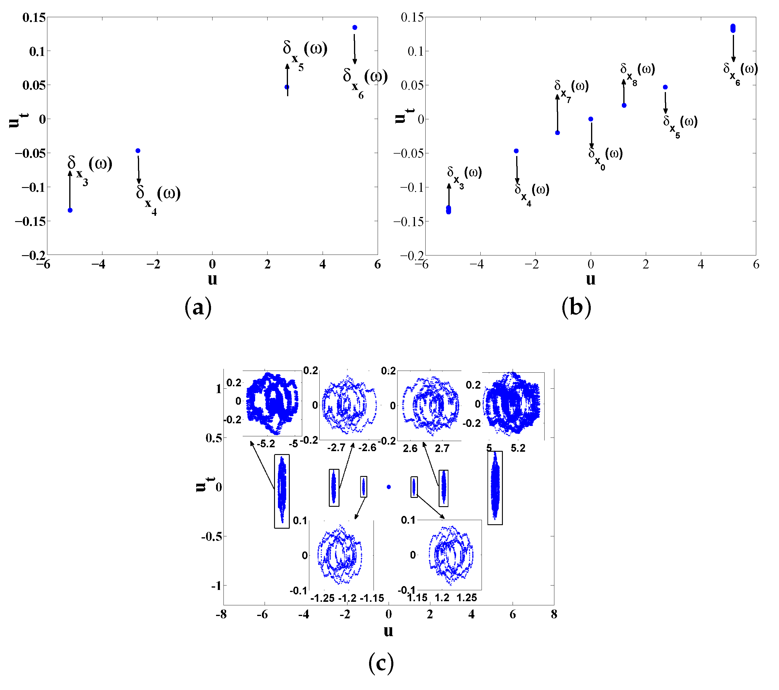
Case III. let , , Figure 4 describes the invariant measures and random attractors for SAVKP. Global random basic attractor is equivalent to global random point attractor in this status. Section of global random basic attractor demonstrated by Figure 4a reveals that the steady states of the system comprise four parts, which means that are least four stable invariant Markov measures for SAVKP exist. In addition, in Figure 4a, it can be obtained that the local dynamics of the system may be complex. The sketch of global random basic attractor is shown by Figure 4b,
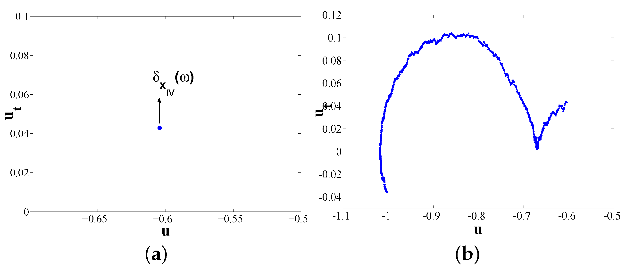
Case IV. when , , global random basic attractor is also equivalent to global random point attractor in this case. The numerical results on the invariant measures and random attractors for SAVKP (see Figure 5) expose the system has a almost surely global stability invariant Markov measure supported by a random fixed points.
The situation of multiplicative white noise. In this case, the P in Figure 1 is equal to , while the remaining parameters are chosen to be the same as in the situation of additive white noise. The the dynamics of SMVKP are studied in the following cases.
Case I. Let , , similar to the Case I in additive noise, global random basic attractor, global random point attractor and global random attractors for SAVKP are the same in this circumstance. The assertion that there exists an almost surely global stability invariant measure supported by a random fixed points for SMVKP can be attained by Figure 6.
Case II. When , , the numerical results on invariant measures and random attractors were described by Figure 7. Invoking the section of global random basic attractor (see Figure 7a), it can be obtained that the system possesses two local stable invariant Markov measures, which together with the numerical results of section global random point attractor described by Figure 7b give that another invariant measure exists, which could even be a unstable invariant Markov measure.
Case III. Set , , Figure 8 expresses the numerical results on global random attractors for SMVKP. The section of global random basic attractor shown by Figure 8a indicates that there exist four local stable invariant Markov measures. Furthermore, SMVKP has another three invariant measures which are interpreted by section of global random point attractor (see Figure 8b). The sketch of global random point attractor is illustrated by Figure 8c.
Case IV. Let , , the similar results in Case IV can be got, the Figure to describe the invariant measure and random attractor is not displayed here.
Some affirmations can be approved by the aforementioned numerical results. For the clamped irrotational inertia Von Karman driven by additive white noise, fixed , let vary from to , the global -bifurcation occurs in the motion of the system. Change the value of to be a big one, such , the dynamical behavior becomes much more interesting. From the view of global dynamics, there exits secondary -bifurcation. The local dynamics of the system is complex. On the other hand, let and change the from to 2, the phenomenon of global -bifurcation disappears. As for clamped irrotational inertia Von Karman driven by multiplicative white noise, fixed , the similar global dynamics of the system can be obtained with varying the from to . In addition, once the coefficient of the multiplicative white noise becomes big, global -bifurcation vanishes. Nevertheless, there exist differences between the two cases above. The multiplicative white noise is more likely to result in the appearance of global -bifurcation and secondary global -bifurcation in the motion of clamped Von Karman without rotational inertia than additive noises. when the secondary -bifurcation occurs, the local dynamics of the system driven by additive white noise is more complex than the situation of multiplicative white noise.
3. Preliminary Results
This section pays attention to give preliminaries and derive certain estimates for solution of SAVKPT1 and SMVKPT1, which are very important to prove main results provided in Section 2.2.
3.1. Basic Theory Related to Global Random Attractors
This subsection is devoted to introduce basic theory related to the theory of random attractors used in this paper.
Proposition 1.
defined by Equation (14) satisfies
and is a stationary Gauss Process and Markov Process, its probability-distribution function induce a Markov semigroup. Furthermore,
and
The sets is tempered with respect to . Moreover, if , then
When , the following holds
Moreover,
where is usual Γ function.
To give the notion of global random attractors, the definition of RDS inaugurated by Arnold [4] is needed to be given firstly.
Definition 1.
([4]) A RDS on Polish space with Borel σ-algebra over a metric dynamical system is a measurable mapping
such that, for , ,
- (i).
- on X.
- (ii).
- for all
A RDS is continuous or differential if is continuous or differential. Furthermore, can be understood as the solution start from to 0.
The coming definitions related to random attractors for RDS was established by Crauel et al. [5,63].
Definition 2.
A random set is said to absorb the set for a RDS if there exists such that
Definition 3.
where dist denotes the Hausdorff semidistance:
Let be a collection of subsets of X, then a closed random set is called -random attractor associated with the RDS ϕ, if
- (i).
- is a random compact set.
- (ii).
- is invariant i.e., for all
- (iii).
- For every ,
When is composed of all bounded set of X, then is the global random attractors for ϕ. If , is said to be global random point attractor.
The next theorem, dedicated to verifying the existence of random attractors for SEBT1 directly, can be derived from Theorem 3.11 in Crauel et al. [5].
Theorem 5.
Suppose ϕ is an RDS on connected Polish space , and suppose that ϕ possesses an absorbing set in X and for any nonrandom bounded set is relatively compact -a.s. Then, ϕ possesses uniqueness global random attractors defined by the following
where union is taken over all bounded , and given by
Furthermore, is measurable with respect to and connected. .
The following assertion provides the relationship between random attractors and invariant measures which is important to expound the global dynamics for RDS was stated in [4,8,63,64].
Proposition 2.
When the RDS ϕ possesses global random attractor comply with Definition 3, by the Corollary 4.4 in Crauel [8], this attractors supports every invariant measures. The random point attractor of ϕ given by Definition 3 always supports at lest one invariant measure which even is a invariant Markov measure (Crauel [63], P423; Arnold [4], Theorem 1.6.13 and Theorem 1.7.5). When ϕ is a white noise RDS or SDS, together with the Theorem 3.6 in Crauel [63] give that every invariant Markov measure is supported by the global point attractor. On the other hand, if the global random attractors for ϕ exists, then ϕ also has the global point attractor. For any fixed , taking advantage of pullback mechanism [4], follow the proof of Theorem 5.2 in Birnir [64], the global random attractor can be decomposed into two ingredients, one is random basic attractor which supports all stable invariant Markov measures of white noise RDS, the other is random remainder. For the definition of basic and remainder, we refer to Birnir [64].
With the assertion that the RDS possesses a global random attractors, in light of Proposition 2, the investigation on global dynamics of RDS can be accomplished by exploiting the numerical results on the structure of global random attractor.
The next proposition should be used in checking that the RDS satisfies condition “for any nonrandom bounded set , is relative compact -a.s.” in Theorem 5.
Proposition 3.
([26]) Suppose is any bounded set, let
then is known as the Kuratowski’s α-measure of non-compactness of B, in short, α-measure of B, which has the following properties.
- (i)
- if and only if B is pre-compact.
- (ii)
- .
- (iii)
- .
- (iv)
- , where is the closed convex hull of B.
- (v)
- If are nonempty closed sets in X such that as , then is nonempty and compact.
3.2. Main Estimates
This subsection presents the main estimates for the solutions of the systems and some lemmas that are momentous to derive the proof for main results.
Firstly, the following properties on Von Karman bracket were given by Proposition 1.4.2 in Chueshov and Lasiecka [26].
If either at least on of belongs to or all of them belong to , then
If , then
The next Lemma consider the sharp regularity Von Karman bracket.
Lemma 1.
The assertion that the condition “D is a bounded domain with regular boundary or a rectangle in ” can be relaxed to “D is a bounded domain satisfies cone property in ”, which can be derived using the property of continuation in Sobolev space [65].
The coming Lemma reveals a relationship between Airy function and in-plane force .
Lemma 2.
Proof.
See the Appendix B.1. ☐
According to Lemma 2, the following estimates which play a crucial role in obtaining the existence of global absorbing set for vibration of Von Karman with a arbitrarily small coefficient of weakly damping.
Let be the solution of SAVKPT2 or SMVKPT2, satisfies (23), define
Combining Lemma 2 with Equations (10e)–(10h), we have
then
where is any given positive, is a positive, which is inversely proportional to . In addition, invoking the trace theorem [57], we attain
In contrast to Inequality (9.1.17) provided by Lemma 9.1.7 in Chueshov and Lasiecka [26], the inequality in Equation (45) give a clear relationship between and the in-plane force , which along with Equation (46) indicates that is determined by the component of the in-plane force on boundary along the direction .
Since the form of damping is weak and the coefficient of it can be arbitrarily small, it is accomplished by verifying the condition in Theorem 5 that “for any nonrandom bounded set is relative compact -a.s.” relies on the stabilization estimation of the considered systems. The results listed in the next two Lemmas are very important to accomplish the stabilization estimation of SAVKPT1 and SMVKPT1.
Lemma 3.
Suppose , are two given bounded sequences, which are weakly star convergence to , respectively. Then, for , the following holds
Lemma 4.
Suppose , are two given bounded sequences, which are weakly star convergence to , respectively. Then, for , the following holds
Lemma 3 was proposed by Khanmamedov [35]. With a similar treatment, the results in Lemma 4 can be attained. Hence, it is omitted it here.
It is noticed that the in Equations (15) and (20) are the same, then the estimates given in the next Lemma, which can be obtained by simple computation, should be employed in both cases of additive white noise and multiplicative white noise.
Lemma 5.
The following Lemmas are used to prove the existence and uniqueness of solutions for SAVKP and SMVKP by semigroup theory.
Lemma 6.
Proof.
See Appendix B.2. ☐
Base on the Lemma 6, the ensuring results focus on eigenvalues of can be verified.
Lemma 7.
The eigenvalues of are as follows.
Proof.
See Appendix B.3. ☐
3.2.1. Main Estimates Only Be Valid in Situation of Additive White Noise
This subsubsection is to give main estimates that only be valid in additive white noise case.
For any given , for , by Reference [26], we have there exists constant , such that
along with Equation (50), we have
where is a constant.
Employing Young’s inequality, it can be obtained that
The next lemma shows possesses global random absorbing set in . In addition, the expectation of radius of this random set is bounded.
Lemma 8.
For any given non random bounded set , there exists , such that, for , the following holds -a.s.
and . In which and are formulated by Equations (26) and (27), respectively.
Proof.
See Appendix B.4. ☐
Let ; based on Lemma 8, it can be obtained that, for any non-random bounded set , there exists , such that, for , the following holds
The coming lemma plays a key role in verifying the condition in Theorem 5 that “for any nonrandom bounded set is relative compact -a.s.” which is significant to prove the existence of the global random attractors for SAVKPT1.
Lemma 9.
Suppose is any given bounded sequence in any given non-random bounded set , is a any given constant, . Then, for , there exist and such that
and
Proof.
See the Appendix B.5. ☐
3.2.2. Main Estimates Only Be Valid in Situation of Multiplicative White Noise
For any given , , , , is constant, take account into is continuous in , merging with Equation (50), we have that there exists a constant such that
which indicates that satisfies Lipschtiz condition.
The coming Lemma asserts that possesses global random absorbing set in .
Lemma 10.
Let be any given non-random bounded set, then there exists such that
and
where is formulated by Equations (30) and (32), respectively. M is given in Theorem 4.
Proof.
See Appendix B.6. ☐
Let , invoke Lemma 10, we have that for any given bounded set , there exists , such that for , the coming holds
Similar to the results presented in Lemma 9, the stabilization estimation of SMVKPT1 provided in the next Lemma can be derived.
Lemma 11.
Suppose is any given bounded sequence in any given non-random bounded set , is a any given constant, . Then, for , there exist and such that
and
Proof.
See Appendix B.7. ☐
4. Proofs for Main Results
4.1. Proof for Theorem 1
Along with Lemmas 5–7, we have can induce a linear semigroup of contractions denoted by . Invoking Equation (51), we get satisfies the Lipschtiz condition. is continuous in . Hence, according to Theorem 2.5.1 in Reference [66], we conclude that SAVKP possesses uniqueness (mild) solution with the form
where, . Thus,
Let , we have
Therefore,
Hence, is the value of a solution for Equation (10a) with initial value at time t. Then
Furthermore, the solution mapping satisfies
On the other hand, which means . Thus, the proof is completedf.
4.2. Proof for Theorem 2
It follows from Lemma 8 that the RDS possesses global absorbing set in . The estimation of expectation of radius of the global absorbing set is obtained in the proof for Lemma 8 if the condition that “for any nonrandom bounded set is relative compact -a.s.” can be satisfied, which is achieved in the following. Then, according the Theorem 5, we can complete the proof of this theorem.
Suppose is any bounded set, let and
From Reference [67], we have
and is nonempty closed set.
Let , then
In the following, we verify is relative compact. It is enough to prove
where denote the measure.
Taking advantage of the contradiction method, suppose Equation (70) is not true, then there exists , for and such that
Let , obviously, . Hence, which reveals that there exists sequence such that
which contradicts Equation (59). Thus, the supposed assumption is invalid which means Equation (70) holds. Then, which means , together with (69), by the Proposition 3, we have is compact. On the other hand, since
Let
then is compact.
According to Theorem 5, it can be found that the RDS possesses random attractors defined by
4.3. Proof for Theorem 3
By Equation (60), we have satisfies Lipschtiz condition, and the rest of proof is very similar to the Proof for Theorem 1 provided in Section 4.4. Thus, it is omitted here.
4.4. Proof for Theorem 4
5. Summary and Conclusions
The affirmation that expectation of radius of global random attractors for nonlinear stochastic plates considered in the paper is in direct proportion to the intensity of white noise and can be derived by Theorem 2 and Theorem 4. On the other hand, it follows from Theorem 4 and the assumption in Equation (28) that, for the clamped Von Karman plate without rotational inertia driven by multiplicative white noise, values for the coefficient of the noise that are too large might result in the non-existence of global random attractor for the system, the phenomenon of which cannot be obtained in the status of additive white noise. The estimate of Equation (45) is derived in Section 3.2 to achieve the existence of global absorbing set for the system, which can also accomplished by Inequality (9.1.17) provided by Lemma 9.1.7 in Chueshov and Lasiecka [26]. However, the inequality in Equation (45) gives a clear relationship between defined by Equation (44) in Section 3.2 and the in-plane force , which along with Equation (46) indicates that is determined by the component of the in-plane force on boundary along the direction . This assertion can expounds the bucking phenomenon from the theoretical results on global random attractors.
Compared with the results on global attractors provided by Chen et al. [36] in situation of multiplicative noise, the investigation on existence of global random attractors for the systems, which are carried out in this paper, do not need the assumption that coefficient of the damping is big enough. This statement can be achieved by the process of proving the existence of global random absorbing set for clamped Von Karman plate without rotational inertia driven by white noise (see Lemma 8 in Section 3.2.1 and Lemma 10 in Section 3.2.2) and attaining the stabilization estimation of the systems(see Lemma 9 in Section 3.2.1 and Lemma 11 in Section 3.2.2). It is noticed that the condition for the existence of global random attractors presented by Chen et al. [36] is so conservative that, once there does not exist a steady ingredient of the loading, which means in the governing equations of Von Karman plate considered in [36], then the global random attractors only comprise the random fixed points (even the trivial solution). It is led by the too big coefficient of damping. The results obtained in this paper indicate that there exists global random attractors for the systems with the small coefficient of weak damping. Moreover, the statement that global random attractors are composed of more than a fixed random point is illustrated by the numerical results on global dynamics. On the other hand, the conclusion that multiplicative white noise is more likely to result in the appearance of global -bifurcation and secondary global -bifurcation in the motion of clamped Von Karman without rotational inertia than additive noises can also be validated from the numerical results on global dynamics of the systems.
In engineering applications, are the in-plane components of the external force that act on the edge of the plate. In light of Equations (3) and (4) given in Section 2.1, with Equation (46) attained in Section 3.2.1, the boundary value of and are determined by . Thus, the aforementioned qualitative results on long time behavior for the two kinds of nonlinear stochastic Von Karman plates are demonstrated by the numerical results on global dynamics. Big enough value of external force that acts on the edge of the plate leads to the appearance of global -bifurcation in the motion of the simplified Von Karman plate without rotational inertia, which coincides with the phenomena named bucking [1]. Furthermore, the fact mentioned above together with assertion that global -bifurcation would disappear with increasing the value of intensity of the white noise can give a reasonable explanation of how the random snap-through [68] occurs in motion of the stochastic Von Karman plate and how to eliminate it in the following manner. When the global random attractor only comprise a fixed random point, then random snap-through occurs. Once the global -bifurcation appears in the motion of the Von Karman plate, the random snap-through will disappears. Alternatively, the large value of the intensity of the white noise results in the occurring of the random snap-through which can be eliminated by increasing the value of external force that act on the edge of the plate. As indicated above, it can be concluded that the random snap-through which seems to be a complex dynamics intuitively is essentially a simple dynamical behavior.
Author Contributions
Conceptualization, Investigation, Writing—Original Draft Preparation, and Writing—Review and Editing, H.C.; Investigation, Supervision, Project Administration, Funding Acquisition, and Writing—Review and Editing, D.C.; Investigation, Writing—Review and Editing, J.J.; Resources; and Writing—Review and Editing, X.F.
Funding
This work was supported by the Key Project of National Natural Science Foundation of China (No. 11732005) and the National Natural Science Foundation of China (No. 91216106, 11472089).
Conflicts of Interest
The authors declare no conflict of interest.
Abbreviations
| RDS | Random Dynamical System |
| SAVKP | The system described by Equations (10a), (10c), (10e)–(10h) |
| SAVKPT1 | The system described by Equations (10c), (15) and (10e)–(10h) |
| SAVAPT2 | The system described by Equations (18), (10c) and (10e)–(10h) |
| SMVKP | The system interpreted by Equations (10b), (10c), (10e)–(10h) |
| SMVKPT1 | The system interpreted by Equations (20), (10c) and (10e)–(10f) |
| SMVAPT2 | The system interpreted by Equations (21), (10c) and (10e)–(10f) |
Appendix A. The Model Equation
Suppose ,, where are eigenvectors related to eigenvalues of operator A. Taking the inner product of Equation (10e) by in , we have
then
Thus, the model equations associated with SAVKP have the following form
where represents the low-frequency modal and the other is high-frequency modal , is the value of at time i. . h is step size of numerical integration. is an undetermined constant.
and
in which
Furthermore, let
then, respectively, replacing in Equation (A1) by leads to the modal equations for SMVKP.
Appendix B. Proof of the Lemmas in Section 3
Appendix B.1. Proof of Lemma 2
Since
together with Equation (10f) gives
Taking into account Equation (10g), we have
Appendix B.2. Proof of Lemma 6
Let , define
where . By Cauchy inequality, there exists such that
From the Proofs of Lax–Milgram given by Temam [55], we have
where is the conjugate space of . Moreover, Equation (49) yields
Let
then . Since , then (A5) yields .
Furthermore, Invoking Equation (A6), this gives is injection. On the other hand, since , by applying (A5), we have is surjection. By open mapping theorem, we obtain that the inverse of exists and .
Appendix B.3. Proof of Lemma 7
Without loss of generality, suppose is eigenvector with respect to eigenvalues , then
Thus,
Equation (A8) yields ; substituting it into Equation (A9), we have
then
Since , we obtain
Hence,
Appendix B.4. Proof of Lemma 8
Taking the inner product of Equation (18) by in gives
According to Lemma 5, we find
It follows from Equations (57) and (58) that the third and fourth term on the right of the inequality sign in Equation (A11) can be controlled by
By means of Equation (52), we catch
It can be derived from Equation (54) that
Let
Invoking Equation (53), we have
which along with Equations (25) and (A11) gives
Setting and then employing Equation (A13), it can be asserted that, for any give ,, the next holds
which means that for any ,
Incorporating Equation (A12), we obtain
Since , , then
By Equation (34), we have that there exists , such that for , the following holds (-a.s.)
furthermore, according to Equation (24), we find , then
Since is tempered, we have
and
Merging with Equation (25), we attain
then defined by Equation (26) is bounded (-a.s.).
It follows from Equations (A15) to (A18) that there exists , such that, for , the following holds
On the other hand, since
let , then, for any non-random bounded set , there exists , such that, for , the following holds (-a.s.)
The rest is intended to estimate the expectation of . Invoking Equation (36), we have
on the other hand,
where is function, which together with Equation (A21) and Cauchy equality gives
Define
in which
Obviously, . In addition, merging with Equations (25) and (A21)–(A23), we have
Appendix B.5. Proof of Lemma 9
For , let
By Lemma 8, we find has a weakly star subsequence in , still denoted by .
Taking the inner product of Equation (16) by in , which, merging with Equation (5) and , gives
where
Since , then
Notice that , then . Let
thus, for , there exists
such that
Set
Since , along with Equation (A26), and Lemmas 3 and 4, we obtain
Appendix B.6. Proof of Lemma 10
Taking the inner product of Equation (21) by in , we have
Invoking Lemma 5, we find
Substituting Equations (A28)–(A29) into Equation (A27), we obtain
along with Equations (66) and (67), we have
Let
applying Equation (53), we attain
according to Equation (A30), we have
where is given by Equation (29) and K is denoted by Equation (31).
It follows form Equation (A32) that
which means that for any given , , the following holds
Since
then, there exits such that for any , the ensuing can be satisfied
which together with Equation (28) gives that ; hence, when ,
therefore
Combining Equation (31) with the fact that is tempered, we have that defined by Equation (29) is a bounded random variable (-a.s.). Furthermore, merging with Equation (A31), we find the random variable in Equation (30) is also bounded.
Incorporating Equation (A40), it can be derived that. for any initial value , there exists such that
Based on the relationship between v and u, we have that. for any initial value , the following holds
Let , ; along with Equation (32), it can be asserted that, for any given non-random bounded set , there exists such that for , the following holds -a.s.
Thus, possesses global random absorbing set in .
The remainder of this proof is intended to estimate the expectation of . It follows from Equations (35), (36) and (29) that
Merging with Equation (A21) and Cauchy inequality, we have
Let
in which
Together with Equations (30), (A41), (A42) and (A37)–(A39), we have
Appendix B.7. Proof of Lemma 11
For , let
By Lemma 10, we find that have weakly star convergence in , still denoted by . Obviously satisfies Equation (22). Taking the inner product of Equation (22) by in , we have
In light of Lemma 5, we have
In term of Equations (61)–(63), we find
Merging with Equation (29), we obtain
Since , then
where is denoted by Equation (A41)
Substituting Equations (A45) and (A46) into Equation (A44), it can be obtained
hence
By Equation (A35), we have that for any given , , the following holds
and
Hence, for any , let
then, it follows from Equations (A50) and (A51) that there exists
such that
where is defined in Lemma 10,
employ the relationship between and , we derive
Let
then
along with Equation (1), we have , which together with Lemmas 3 and 4 gives
References
- Amabili, M. Nonlinear Vibrations and Stability of Shells and Plates; Cambridge University Press: Cambridge, UK, 2008. [Google Scholar]
- Lagnese, J.E. Boundary Stabilization of Thin Plates; SIAM: Philadelphia, PA, USA, 1989. [Google Scholar]
- Ciarlet, P.G. Mathematical Elasticity: Theory of Plates; Elsevier: Amsterdam, The Netherlands, 1997. [Google Scholar]
- Arnold, L. Random Dynamical Systems; Springer: Berlin, Germany, 1998. [Google Scholar]
- Crauel, H.; Flandoli, F. Attractors for random dynamical systems. Probab. Theory Relat. Fields 1994, 100, 365–393. [Google Scholar] [CrossRef]
- Schmalfuss, B. Measure Attractors and Stochastic Attractors, Institut for Dynamische Systeme; Technical Report; Bermen University: Bermen, Germany, 1995. [Google Scholar]
- Crauel, H.; Debussche, A.; Flandoli, F. Random attractors. J. Dyn. Differ. Equ. 1997, 9, 307–341. [Google Scholar] [CrossRef]
- Crauel, H. Global random attractors are uniquely determined by attracting deterministic compact sets. Ann. Mat. Pura Appl. 1999, 176, 57–72. [Google Scholar] [CrossRef]
- Bates, P.W.; Lu, K.; Wang, B. Random attractors for stochastic reaction–diffusion equations on unbounded domains. J. Differ. Equ. 2009, 246, 845–869. [Google Scholar] [CrossRef]
- Caraballo, T.; Langa, J.A.; Robinson, J.C. Stability and random attractors for a reaction-diffusion equation with multiplicative noise. Discret. Contin. Dyn. Syst. 2000, 6, 875–892. [Google Scholar]
- Zhou, S.; Yin, F.; Ouyang, Z. Random attractor for damped nonlinear wave equations with white noise. SIAM J. Appl. Dyn. Syst. 2005, 4, 883–903. [Google Scholar] [CrossRef]
- Fan, X.; Chen, H. Attractors for the stochastic reaction–diffusion equation driven by linear multiplicative noise with a variable coefficient. J. Math. Anal. Appl. 2013, 398, 715–728. [Google Scholar] [CrossRef]
- Fan, X. Attractors for a damped stochastic wave equation of Sine–Gordon type with sublinear multiplicative noise. Stochastic Anal. Appl. 2006, 24, 767–793. [Google Scholar] [CrossRef]
- You, Y. Global Attractor for Nonlinear Wave Equations with Critical Exponent on Unbounded Domain. Appl. Math. Nonlinear Sci. 2016, 2, 581–602. [Google Scholar] [CrossRef]
- Pappalardo, C.M.; Guida, D. Use of the Adjoint Method for Controlling the Mechanical Vibrations of Nonlinear Systems. Machines 2018, 6, 19. [Google Scholar] [CrossRef]
- Fortuna, L.; Muscato, G. A roll stabilization system for a monohull ship: Modeling, identification, and adaptive control. IEEE Trans. Control Syst. Technol. 1996, 4, 18–28. [Google Scholar] [CrossRef]
- Pappalardo, C.M.; Guida, D. System Identification Algorithm for Computing the Modal Parameters of Linear Mechanical Systems. Machines 2018, 6, 12. [Google Scholar] [CrossRef]
- Pappalardo, C.M.; Guida, D. On the Computational Methods for Solving the Differential-Algebraic Equations of Motion of Multibody Systems. Machines 2018, 6, 20. [Google Scholar] [CrossRef]
- Pappalardo, C.M.; Zhang, Z.; Shabana, A.A. Use of independent volume parameters in the development of new large displacement ANCF triangular plate/shell elements. Nonlinear Dyn. 2018, 91, 2171–2202. [Google Scholar] [CrossRef]
- Pappalardo, C.M.; Wallin, M.; Shabana, A.A. A new ANCF/CRBF fully parameterized plate finite element. J. Comput. Nonlinear Dyn. 2017, 12, 031008. [Google Scholar] [CrossRef]
- Pappalardo, C.M.; Yu, Z.; Zhang, X.; Shabana, A.A. Rational ANCF thin plate finite element. J. Comput. Nonlinear Dyn. 2016, 11, 051009. [Google Scholar] [CrossRef]
- Lasiecka, I. Weak, classical and intermediate solutions to full von Kármán system of dynamic nonlinear elasticity. Appl. Anal. 1998, 68, 121–145. [Google Scholar]
- Leiva, H.; Sivoli, Z. Existence, stability and smoothness of a bounded solution for nonlinear time-varying thermoelastic plate equations. J. Math. Anal. Appl. 2003, 285, 191–211. [Google Scholar] [CrossRef]
- Abels, H.; Mora, M.G.; Müller, S. The time-dependent von Kármán plate equation as a limit of 3d nonlinear elasticity. Calc. Var. Partial Differ. Equ. 2011, 41, 241–259. [Google Scholar] [CrossRef]
- Favini, A.; Horn, M.A.; Lasiecka, I.; Tataru, D. Global existence, uniqueness and regularity of solutions to a von Karman system with nonlinear boundary dissipation. Differ. Integral Equ. 1996, 9, 267–294. [Google Scholar]
- Chueshov, I.; Lasiecka, I. Von Karman Evolution Equations: Well-Posedness and Long Time Dynamics; Springer Science & Business Media: Berlin/Heidelberg, Germany, 2010. [Google Scholar]
- Chueshov, I.; Lasiecka, I. Attractors for second-order evolution equations with a nonlinear damping. J. Dyn. Differ. Equ. 2004, 16, 469–512. [Google Scholar] [CrossRef]
- Chueshov, I.; Lasiecka, I. Inertial manifolds for von Kármán plate equations. Appl. Math. Optim. 2002, 46, 179–206. [Google Scholar]
- Lasiecka, I. Uniform decay rates for full von karman system of dynamic theromelasticity with free boundary conditions and partial boundary dissipation. Commun. Partial Differ. Equ. 1999, 24, 1801–1847. [Google Scholar] [CrossRef]
- Ryzhkova, I. Dynamics of a thermoelastic von Karman plate in a subsonic gas flow. Zeitschrift für angewandte Mathematik und Physik 2007, 58, 246–261. [Google Scholar] [CrossRef]
- Yeoul Park, J.; Hye Park, S. Uniform decay for a von Karman plate equation with a boundary memory condition. Math. Methods Appl. Sci. 2005, 28, 2225–2240. [Google Scholar] [CrossRef]
- Park, S.H. Long-time dynamics of a von Karman equation with time delay. Appl. Math. Lett. 2018, 75, 128–134. [Google Scholar] [CrossRef]
- Chueshov, I.; Lasiecka, I.; Webster, J.T. Attractors for delayed, nonrotational von Karman plates with applications to flow-structure interactions without any damping. Commun. Partial Differ. Equ. 2014, 39, 1965–1997. [Google Scholar] [CrossRef]
- Lasiecka, I.; Webster, J.T. Eliminating flutter for clamped von Karman plates immersed in subsonic flows. Commun. Pure Appl. Anal. 2014, 13, 1935–1969. [Google Scholar] [CrossRef] [Green Version]
- Khanmamedov, A.K. Global attractors for von Karman equations with nonlinear interior dissipation. J. Math. Anal. Appl. 2006, 318, 92–101. [Google Scholar] [CrossRef]
- Chen, H.; Cao, D.; Jiang, J. Random Attractors for Von Karman Plates Subjected to Multiplicative White Noise Loadings. In Dynamical Systems: Theoretical and Experimental Analysis; Springer: New York, NY, USA, 2016; pp. 59–70. [Google Scholar]
- Awrejcewicz, J.; Krysko, A. Analysis of complex parametric vibrations of plates and shells using Bubnov-Galerkin approach. Arch. Appl. Mech. 2003, 73, 495–504. [Google Scholar] [CrossRef]
- Alijani, F.; Bakhtiari-Nejad, F.; Amabili, M. Nonlinear vibrations of FGM rectangular plates in thermal environments. Nonlinear Dyn. 2011, 66, 251. [Google Scholar] [CrossRef]
- Park, J.S.; Kim, J.H. Thermal postbuckling and vibration analyses of functionally graded plates. J. Sound Vib. 2006, 289, 77–93. [Google Scholar] [CrossRef]
- Rashidi, M.; Shooshtari, A.; Bég, O.A. Homotopy perturbation study of nonlinear vibration of Von Karman rectangular plates. Comput. Struct. 2012, 106, 46–55. [Google Scholar] [CrossRef]
- Ghayesh, M.H.; Amabili, M.; Païdoussis, M.P. Nonlinear dynamics of axially moving plates. J. Sound Vib. 2013, 332, 391–406. [Google Scholar] [CrossRef]
- Ghayesh, M.H.; Farokhi, H. Nonlinear dynamics of microplates. Int. J. Eng. Sci. 2015, 86, 60–73. [Google Scholar] [CrossRef]
- Amabili, M. Nonlinear vibrations of viscoelastic rectangular plates. J. Sound Vib. 2016, 362, 142–156. [Google Scholar] [CrossRef]
- Wiggins, S. Global Bifurcations and Chaos: Analytical Methods; Springer Science & Business Media: Heidenburg, Germany, 2013; Volume 73. [Google Scholar]
- Feng, Z.; Wiggins, S. On the existence of chaos in a class of two-degree-of-freedom, damped, strongly parametrically forced mechanical systems with brokenO (2) symmetry. Zeitschrift für angewandte Mathematik und Physik ZAMP 1993, 44, 201–248. [Google Scholar] [CrossRef]
- Zhang, W. Global and chaotic dynamics for a parametrically excited thin plate. J. Sound Vib. 2001, 239, 1013–1036. [Google Scholar] [CrossRef]
- Hsu, C. A theory of cell-to-cell mapping dynamical systems. J. Appl. Mech. 1980, 47, 931–939. [Google Scholar] [CrossRef]
- Xu, W.; He, Q.; Fang, T.; Rong, H. Stochastic bifurcation in Duffing system subject to harmonic excitation and in presence of random noise. Int. J. Non-Linear Mech. 2004, 39, 1473–1479. [Google Scholar] [CrossRef]
- Crauel, H.; Flandoli, F. Additive noise destroys a pitchfork bifurcation. J. Dyn. Differ. Equ. 1998, 10, 259–274. [Google Scholar] [CrossRef]
- Esteban, M.; Núñez, E.P.; Torres, F. Bifurcation Analysis of Hysteretic Systems with Saddle Dynamics. Appl. Math. Nonlinear Sci. 2016, 2, 449–464. [Google Scholar]
- Arnold, L.; Bleckert, G.; Schenk-Hoppé, K.R. The Stochastic Brusselator: Parametric Noise Destroys Hoft Bifurcation. In Stochastic Dynamics; Springer: New York, NY, USA, 1999; pp. 71–92. [Google Scholar]
- Wang, B. Existence, stability and bifurcation of random complete and periodic solutions of stochastic parabolic equations. Nonlinear Anal. Theory Methods Appl. 2014, 103, 9–25. [Google Scholar] [CrossRef] [Green Version]
- Schenk-Hoppé, K.R. Random attractors—General properties, existence and applications to stochastic bifurcation theory. Discret. Contin. Dyn. Syst.-A 1998, 4, 99–130. [Google Scholar] [CrossRef]
- Caraballo, T.; Langa, J.A.; Robinson, J.C. A stochastic pitchfork bifurcation in a reaction-diffusion equation. In Proceedings of the Royal Society of London A: Mathematical, Physical and Engineering Sciences; The Royal Society: London, UK, 2001; Volume 457, pp. 2041–2061. [Google Scholar]
- Temam, R. Infinite-Dimensional Dynamical Systems in Mechanics And Physics; Springer: New York, NY, USA, 1997. [Google Scholar]
- Keller, H.; Ochs, G. Numerical approximation of random attractors. In Stochastic Dynamics; Springer: New York, NY, USA, 1999; pp. 93–115. [Google Scholar]
- Lions, J.L.; Magenes, E. Non-Homogeneous Boundary Value Problems and Applications; Springer Science & Business Media: Paris, France, 2012; pp. 7–8, 112–131, 275–276. [Google Scholar]
- Debussche, A.; Temam, R. Some new generalizations of inertial manifolds. Discret. Contin. Dyn. Syst.-A 1996, 2, 543–558. [Google Scholar]
- Marion, M.; Temam, R. Nonlinear galerkin methods. SIAM J. Numerical Anal. 1989, 26, 1139–1157. [Google Scholar] [CrossRef]
- Multiphysics, A. COMSOL Multiphysics 3.5 a Reference Manual, PDE Mode Equation Based Modeling; Multiphysics Ltd.: Stohkholm, Sweden, 2008. [Google Scholar]
- Kloeden, P.; Eckhard, P. Numerical Solution of Stochastic Differential Equations; Springer: Berlin, Germany, 1992. [Google Scholar]
- Schmalfuss, B. Measure attractors and random attractors for stochastic partial differential equations. Stochastic Anal. Appl. 1999, 17, 1075–1101. [Google Scholar] [CrossRef]
- Crauel, H. Random point attractors versus random set attractors. J. Lond. Math. Soc. 2001, 63, 413–427. [Google Scholar] [CrossRef]
- Birnir, B. Basic Attractors and Control; Springer: New York, NY, USA, 2015. [Google Scholar]
- Adams, R.A.; Fournier, J.J. Sobolev Spaces; Academic Press: Cambridge, MA, USA, 2003. [Google Scholar]
- Zheng, S. Nonlinear Evolution Equations; CRC Press: Boca Raton, FL, USA, 2004. [Google Scholar]
- Chepyzhov, V.; Vishik, M. A Hausdorff dimension estimate for kernel sections of non-autonomous evolution equations. Indiana Univ. Math. J. 1993, 42, 1057–1076. [Google Scholar] [CrossRef]
- Crisfield, M. A fast incremental/iterative solution procedure that handles “snap-through”. In Computational Methods in Nonlinear Structural and Solid Mechanics; Elsevier: New York, NY, USA, 1981; pp. 55–62. [Google Scholar]
Figure 1.
The model for vibration of Von Kaman plate under the random loading.

Figure 2.
Invariant measures and random attractors for SAVKP in Case I.: (a) invariant measure and section of global random basic attractor; and (b) global random basic attractor.
Figure 2.
Invariant measures and random attractors for SAVKP in Case I.: (a) invariant measure and section of global random basic attractor; and (b) global random basic attractor.

Figure 3.
Invariant measures and random attractors for SAVKP in Case II: (a) invariant measures and global random basic attractor; (b) section of global random attractor; and (c) global random basic attractor.
Figure 3.
Invariant measures and random attractors for SAVKP in Case II: (a) invariant measures and global random basic attractor; (b) section of global random attractor; and (c) global random basic attractor.

Figure 4.
Invariant measures and random attractors for SAVKP in Case III: (a) invariant measure and section of global random basic attractor; and (b) global random basic attractor.
Figure 4.
Invariant measures and random attractors for SAVKP in Case III: (a) invariant measure and section of global random basic attractor; and (b) global random basic attractor.

Figure 5.
Invariant measures and random attractors for SAVKP in Case IV: (a) invariant measure and section of global random basic attractor; and (b) global random basic attractor.
Figure 5.
Invariant measures and random attractors for SAVKP in Case IV: (a) invariant measure and section of global random basic attractor; and (b) global random basic attractor.

Figure 6.
Invariant measures and random attractors for SMVKP in Case I: (a) invariant measure and section of global random basic attractor; and (b) global random basic attractor.
Figure 6.
Invariant measures and random attractors for SMVKP in Case I: (a) invariant measure and section of global random basic attractor; and (b) global random basic attractor.

Figure 7.
Invariant measures and random attractors for SMVKP in Case II: (a) invariant measure and section of global random basic attractor; and (b) global random basic attractor.
Figure 7.
Invariant measures and random attractors for SMVKP in Case II: (a) invariant measure and section of global random basic attractor; and (b) global random basic attractor.

Figure 8.
Invariant measures and random attractors for SMVKP in Case III: (a) invariant measures and global random basic attractor; (b) section of global random point attractor; and (c) global random point attractor.
Figure 8.
Invariant measures and random attractors for SMVKP in Case III: (a) invariant measures and global random basic attractor; (b) section of global random point attractor; and (c) global random point attractor.

© 2018 by the authors. Licensee MDPI, Basel, Switzerland. This article is an open access article distributed under the terms and conditions of the Creative Commons Attribution (CC BY) license (http://creativecommons.org/licenses/by/4.0/).
Share and Cite
MDPI and ACS Style
Chen, H.; Cao, D.; Jiang, J.; Fan, X. Long Time Behavior and Global Dynamics of Simplified Von Karman Plate Without Rotational Inertia Driven by White Noise. Symmetry 2018, 10, 315. https://doi.org/10.3390/sym10080315
AMA Style
Chen H, Cao D, Jiang J, Fan X. Long Time Behavior and Global Dynamics of Simplified Von Karman Plate Without Rotational Inertia Driven by White Noise. Symmetry. 2018; 10(8):315. https://doi.org/10.3390/sym10080315
Chicago/Turabian StyleChen, Huatao, Dengqing Cao, Jingfei Jiang, and Xiaoming Fan. 2018. "Long Time Behavior and Global Dynamics of Simplified Von Karman Plate Without Rotational Inertia Driven by White Noise" Symmetry 10, no. 8: 315. https://doi.org/10.3390/sym10080315
Note that from the first issue of 2016, this journal uses article numbers instead of page numbers. See further details here.