Assessment and Performance Evaluation of a Wind Turbine Power Output


1
School of Energy and Environment, City University of Hong Kong, Hong Kong, China
2
Guy Carpenter Asia-Pacific Climate Impact Center, School of Energy and Environment, City University of Hong Kong, Hong Kong, China
*
Author to whom correspondence should be addressed.
Energies 2018, 11(8), 1992; https://doi.org/10.3390/en11081992
Submission received: 12 June 2018
/
Revised: 25 June 2018
/
Accepted: 26 June 2018
/
Published: 1 August 2018
(This article belongs to the Collection Wind Turbines)
Abstract
:Estimation errors have constantly been a technology bother for wind power management, often time with deviations of actual power curve (APC) from the turbine power curve (TPC). Power output dispersion for an operational 800 kW turbine was analyzed using three averaging tine steps of 1-min, 5-min, and 15-min. The error between the APC and TPC in kWh was about 25% on average, irrespective of the time of the day, although higher magnitudes of error were observed during low wind speeds and poor wind conditions. The 15-min averaged time series proved more suitable for grid management and energy load scheduling, but the error margin was still a major concern. An effective power curve (EPC) based on the polynomial parametric wind turbine power curve modeling technique was calibrated using turbine and site-specific performance data. The EPC reduced estimation error to about 3% in the aforementioned time series during very good wind conditions. By integrating statistical wind speed forecasting methods and site-specific EPCs, wind power forecasting and management can be significantly improved without compromising grid stability.
1. Introduction
Conventionally, energy from multiple sources, such as coal, natural gas, nuclear power, wind, and tides, goes from a power plant to an electrical grid or network for some form of storage, stabilization, and regulation before eventual transmission and distribution through substations to end users. For fossil fuels and non-renewable energy sources, the actual energy input into the grid per unit time is known hence “static”, while that of renewable sources is “dynamic”. Typically, the energy profile includes three major parts: base load, middle load, and peak load [1]. One major challenge of limiting wind power diffusion is that wind sources cannot serve as a base load due to intermittency [1,2,3,4,5]. Since the base load is that fraction of total energy demand that must be available constantly to avoid power outage, it must be static. In energy surplus conditions where supply exceeds demand, the challenge for wind energy is one of optimization. For energy deficit conditions when demand exceeds supply, maximizing wind power input into the grid and meeting energy demand are key.
The relationship between wind speed and wind power based on the wind power equation is described by a turbine specific non-linear transformation curve termed turbine power curve (TPC) and is turbine-specific. One method of wind resource assessment is to fit the wind speed characteristics of the select location into the Weibull distribution probability distribution function (PDF). The frequency of occurrence of different wind speed bins obtained from the PDF is then used to estimate the total power generated for the corresponding wind speed and time duration [5,6]. The sum of all the bins is the total estimate of wind energy output for such a study site. Another method is to use the wind power density (WPD), which does not consider the turbine characteristics, but rather gives an estimate of the available wind power based on wind speed only [7]. Both methods are capable of expressing long-term estimates, which has been shown to sometimes vary from actual field observations. For example, wind speed and power pairs collected from an observational 800 kW wind turbine show deviations of the measured power output (referred to as the actual power curve henceforth APC) from the TPC creating a dispersion belly [8]. Similar dispersion in other studies [3,5,6,9] suggest that if the time series were extracted, APC fluctuations would make estimations of wind energy source input into the electrical grid a technical problem for energy grid operators. Table 1 shows some reviewed studies that have identified fluctuations of the TPC from the APC. Specifically, the turbine model, location, time steps considered, and scope of studies are included in the table. Although there are marked differences in these deviations, the surveyed studies all point to occurrence of deviations occuring irrespective of turbine location, turbine type or specific climatic conditions.
Wind turbine control system operators require wind speed prediction times in the range of seconds ahead. Wind speed prediction can be via numerical weather prediction (NWP) methods as summarized in previous works [17,18,19] and [1] who developed an adaptive neural fuzzy inference system (ANFIS) for wind speed forecasting. Another approach is through statistical methods as described in Reference [3] and used in Reference [8] to develop a linear prediction model effective for wind speed forecasting or the fractionally-integrated Auto-Regressive Integral and Moving Average (f-ARIMA) method adopted in Reference [20]. Statistical methods are ideally suited for short-term predictions, and common forms include regression based methods such as auto-regressive (AR), auto-regressive and moving-average, (ARMA) [21], auto-regressive integral and moving-average (ARIMA) [22]; exponential smoothing (single or double); the persistence model; and neural network fitting (Artificial Neural Network). However, studies on wind speed prediction still continue because there does not seem to be any industry-wide accepted, short-term wind forecasting system for wind power. While studies on wind power and wind turbine performance exists (see Table 1), more recently the use of stochastic models for wind power related studies have increased. Wind turbine fatigue load estimation was conducted by Reference [23] using a stochastic model, especially in wind farms, a condition that is certain to affect turbine performance and power output. In Reference [24], actual measured data was used to construct a stochastic model to monitor wind turbine vibrations and could prove significant for understanding and monitoring turbine operations/maintenance. As regards to the operation and control of turbines, better modeling that incorporates wind uncertainty and accommodates deviations from “normal” turbine working conditions [25] are essential for performance characterization and fault diagnosis. Such better modeling is seen in Reference [26] where a stochastic approach was applied to model energy conversion and power production from a wind farm under various wind conditions including turbulent wind fluctuations. In another dimension, Reference [27] combined a computational fluid dynamic (CFD) approach with blade element momentum (BEM) theory to propose operating conditions for wind turbines during icing conditions.
When errors from wind power estimation occur, the base load may have to be increased [28], and large amounts of usable wind energy may have to be disposed of [29]. In addition, power outages may occur while financial losses in the energy market would be incurred [30]. Ultimately, grid systems may be jeopardized, thereby affecting energy quality and stability [3]. Thus, a combination of approaches from previous studies is adopted to analyze actual turbine performance and its impact on grid input. Measurements from a single turbine such as conducted by References [3,13] is used to investigate the occurrence of very short-term wind variation and turbine power output similar to the studies by References [15,16]. Three different time-steps and averaging times greater than 10 s intervals used by Reference [15], but less than 1 h used by Reference [5] was adopted. This was then extended to investigating estimation errors and possible methods for reducing these errors based on a form of polynomial curve belonging to the parametric modeling technique of wind power curves seen in Reference [31]. The results from this study will be of significant interest for electrical grid management, wind power optimization, and wind turbine controllers and operators, as well as the wind energy industry. First, insight into the time series of wind power estimation is provided for energy grid operators who play an essential role in ensuring an uninterrupted power supply and maintaining grid quality. Second, the analysis provides real-time information for wind turbine controllers to guide decision making in short-term time scales during turbine operation, as opposed to previous studies that provided such information in the range of 1 h, 6 h, or even daily. Third, by investigating estimation errors, the wind energy industry is able to overcome some of the marketing and policy challenges affecting wind power optimization and diffusion.
2. Data and Methodology
Wind speed and wind power pairs for an operational wind turbine were sourced in 15 s intervals for a period of 14 days each for 2 seasons. The first set of measurements were taken in August 2016, representative of the summer season, while the second set was collected in February 2017, representative of the winter season. The turbine is located on a hill approximately 440 m above mean sea level, a Nordex N-50 800 kW turbine with a hub height of 46 m. The coefficient of performance (Cp) ranged from 35% at low wind speed to about 45% at between 5 m/s and 10 m/s, before gradually reducing to about 21% at wind speed above 10 m/s (see Figure S1). The turbine serves mostly for educational and demonstration purposes with real time performance data available.
For the two periods considered, the dataset was initially divided into two parts (dataset A and dataset B) for both summer and winter measurements. The first dataset, comprising about 80% of the datasets, was used for aggregation into 1-min, 5-min, and 15-min time steps using the mathematical notation below.
Three case scenarios were established to typify possible variations of daily wind speed irrespective of time of day using 60 time steps per scenario.
- Scenario A–u > 3.0 from t1–t60:Wind speed range above cut-in speed for the 60 time steps
- Scenario B–u < 3.0 at t1:Wind speed startup lower than cut-in speed
- Scenario C–u > 3.0 between t1–tn, u < 3.0 at tn+1:A range of lower wind speed between higher values
where t1 = time step 1, tn = time step at arbitrary time n, and tn+1 = wind speed at the next time step after time tn; all scenarios were considered using 60 time steps.
The actual power curve (APC) is derived from the wind power values recorded from the corresponding speed for the time series by taking the instantaneous power output from the turbine. The turbine power curve (TPC) is obtained by using a nonlinear transformation function for wind power as stated in two below. It is important to state here that the TPC can actually be divided into three regimes, the non-linear (also cubic) transformation of wind speed to wind power when incident wind speed ranges between 3.0–15 m/s, the linear regime during which the power output is constant for a rated wind speed of 15–25 m/s, and the saturated regime where power output is negligible due to turbine shut-down for too high wind speeds greater than 25 m/s.
To minimize estimation errors, an effective power curve (EPC) was proposed for the performance evaluated using the following criteria: mean absolute error (MAE), mean square error (MSE), and root mean square error (RMSE) [32].
3. Results and Discussion
Power output based on the APC, which is the actual turbine output per time step, and the TPC, which is the power output estimated using the wind power expression were compared. The APC and TPC for each scenario previously defined were considered using 60 time steps t1–t60 for the winter and summer data, respectively, for 1-min, 5-min, and 15-min time intervals. Statistical details describing the wind speed distribution for each of the scenarios and time intervals are provided in Table 2.
3.1. Scenario A
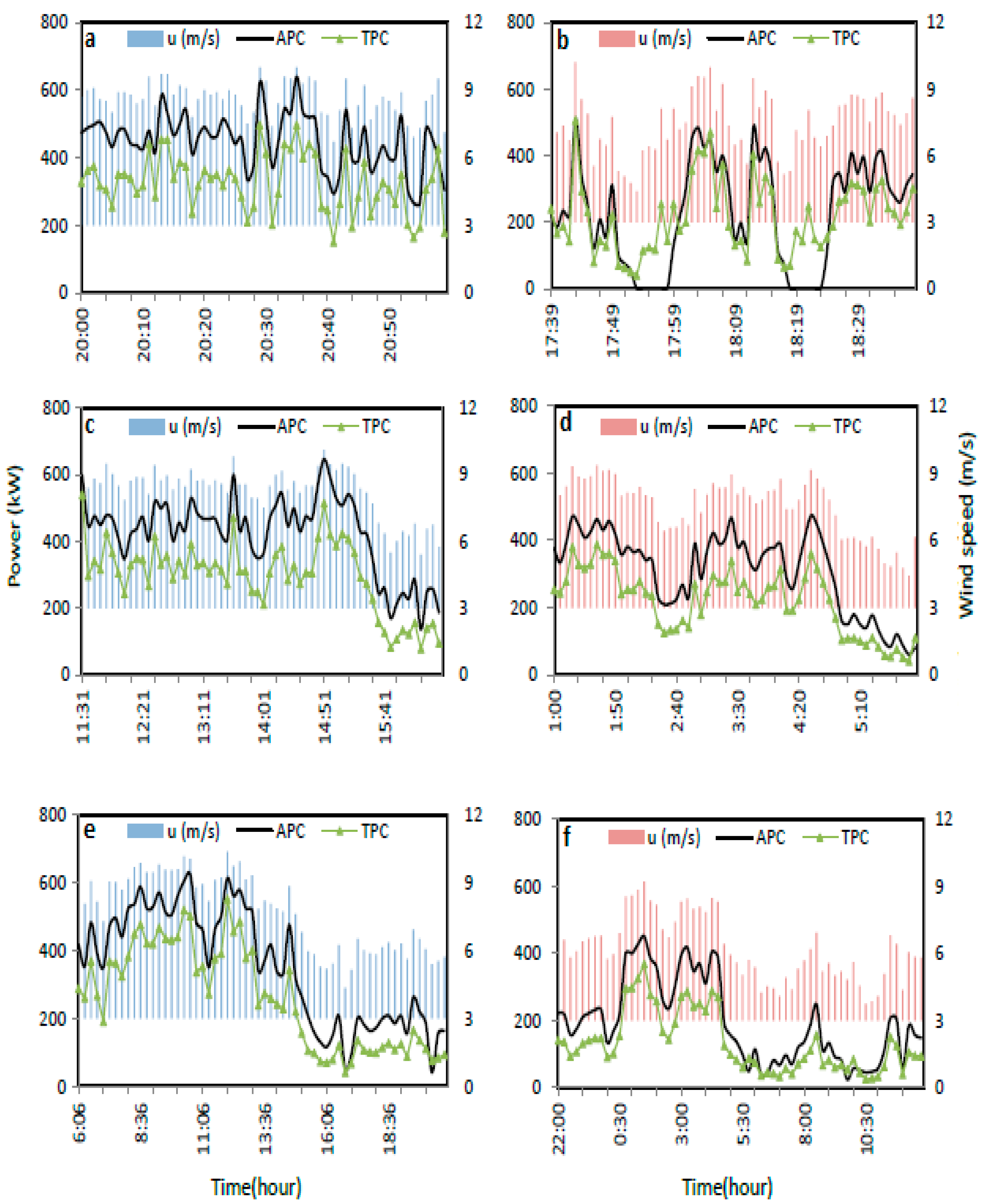
Figure 1a (upper left) shows the APC and TPC at 1-min time intervals during winter from 20:00 to 20:59 hours. The pattern of the APC is accurately captured by the TPC, although TPC underestimated the APC throughout the one hour duration. Compared to Figure 1b, the estimation errors observed in summer were of a lesser magnitude, with two occurrences of overestimation lasting for about 4–5 min each. In both cases the output from the turbine is negligible, almost equivalent to the output during a turbine downtime period. This occurred when instantaneous wind speed was greater than the cut-in speed of 3 m/s required for power generation. Relatively wind speed in winter appeared less dynamic than in summer, although they were measured at different hours of the day. The total energy yield at the end of the hour is 449.3 kWh and 227.5 kWh compared to the theoretical estimate of 324.4 kWh and 215.5 kWh for winter and summer, respectively.
For the 5-min time interval, a similar pattern is observed, with the TPC constantly below the APC for all time steps in winter, as illustrated in Figure 1c. The magnitude of the estimation errors for the individual time steps increased as wind speed reduced and vice versa, although this may be due to averaging rather than a performance issue. The delays in the response time of the wind turbine to fluctuations in wind speed were diminished in this time series, probably as an effect of the averaging. In Figure 1d (middle left) the APC is above the TPC at t60, thus an overestimation. Also, estimation errors appeared to be comparatively less at lower wind speeds and greater at higher wind speeds. For the span of 5 h, the total energy yield was 2125.1 kWh and 1095.9 kWh for winter and summer, respectively. These values are greater than the TPC estimations by 30% and 29%, respectively.
In the case of the 15-min time interval, the first observation was that for each time step estimation errors were less compared to the time series earlier discussed. From Figure 1e,f, it can also be observed that at the same average wind speed, the APC is slightly higher in winter than in summer. This suggests that turbine performance may be significantly affected by season. Mathematically, the wind power expression factors in air density, which is in turn affected by temperature. However, there is limited proof in studies attempting to quantify or measure this impact on wind resource assessments or yield which may form a probable hypothesis for future work. There are notable periods of overestimations of turbine yield by the TPC, although for only about 4–5 time steps. Winter values were from 6:00–19:00 hours to yield 5388.4 kWh, while summer values were from 22:00 hours to 11:00 hours (next day), yielding 2904.9 kWh of energy.
3.2. Scenario B
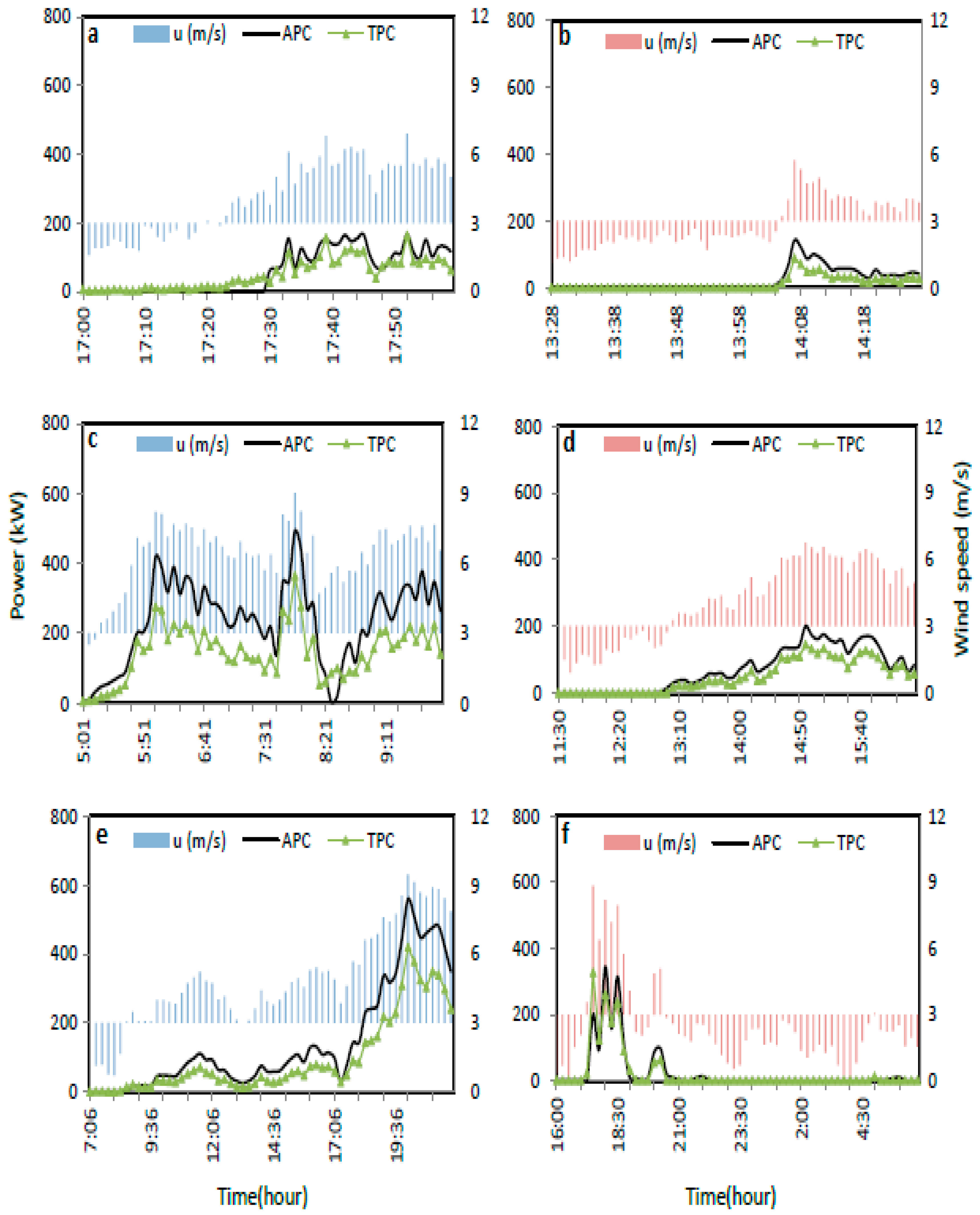
The 1-min time series are shown in Figure 2a,b for winter and summer, respectively. A similar underestimation of the power generated by the TPC is also observed. The estimation error is of lesser magnitude when wind speed is gradually rising, relative to when wind speed falls. The performance in winter is also slightly higher than in summer, although the hour of the day varied for both seasons. There is a noticeable delay of about 8–10 min in power production for the wind turbine in 2a despite wind speed being above the cut-in speed. This suggests that wind direction and/or turbine inertia may affect energy production, especially during poor wind conditions. Wind direction however is a stochastic property and technically challenging to predict in short time scales. Energy yield was underestimated at the end of the hour by 14% (43%) for winter (summer).
The 5-min interval time series shown in Figure 2c,d are quite similar to those of the 1-min interval. There was an overestimation by the TPC for about four time steps since in these instances the actual power generated was negligible. As highlighted earlier, less deviation of the TPC from the APC was observed when wind speed gradually increased, in contrast to when wind speed decreased or when there are abrupt changes in the magnitude of wind speed. There are minimized occurrences of lags and delays, perhaps due to the averaging of the series. Overall estimation error in this case was generally lower compared to scenario A because of a considerably lower turbine operation time. Total yield in winter was 1164.5 kWh, while that in summer was 353.0 kWh, compared to theoretical estimates of 733.0 kWh and 249.3 kWh, respectively.
In the 15-min interval time series shown in Figure 2e,f, the APC and TPC appeared to respond immediately to changes in wind speed and are less sensitive to abrupt variations. Also, delays and lags are completely eliminated due to the averaging. A period of poor wind speed was observed in summer (Figure 2f) which lasted for over 6 hours. This is undesirable for wind power production, as it would impact energy supply and grid quality, putting customers at risk of power outages. Also, this spell means that estimation error would be relatively lower, since again total turbine operational time was less. Energy yield for the 60 time steps was 2510.5 kWh and 390.6 kWh for winter and summer respectively, corresponding to an overestimation of summer wind power by 3%.
3.3. Scenario C
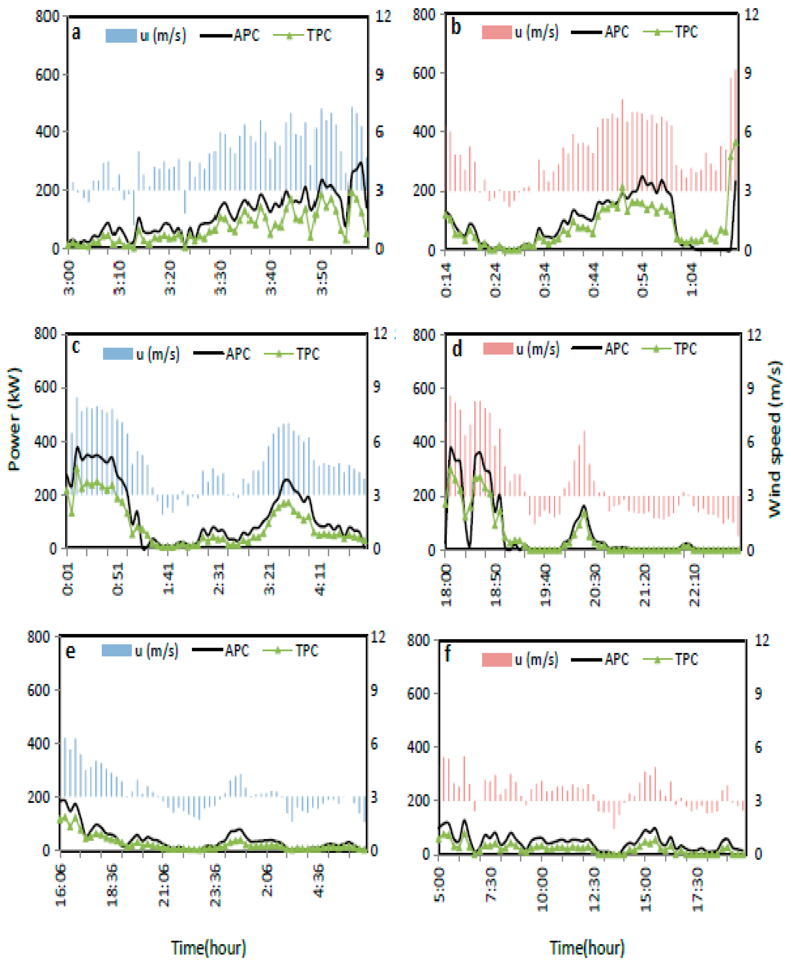
For times where wind speed varied between less than and greater than 3.0 m/s for a short time spans, turbine yield is sustained, as seen in winter in Figure 3a. From t2–t5 and from t11–t15, wind speed was less than 3.0 m/s although power was generated by the turbine. There was, however, a considerable reduction in power output in the latter case. Variation in wind speed is mirrored by the APC and TPC for most of the remaining time steps. The summer test in Figure 3b also shows a pattern similar to those of winter, except between t50 and t58 where the APC is negligible. This again suggested that wind direction and turbine inertia may affect turbine yield, especially during wind conditions. The TPC underestimated yield by 39% and 9% after the 1 h sampled for winter and summer, respectively.
For the winter 5-min interval time series seen in Figure 3c, the actual yield by the APC was considerably higher than the TPC for most of the initial time steps when wind speed was greater than 6.0 m/s. A sharp decline of power output was also observed in summer (see Figure 3d) despite average wind speed being slightly above the cut-in speed. For both seasons, there were instances of negligible power generated by the turbine, attributable to poor wind speed, changes in wind direction, or the effect of time-series averaging. The total yield from the APC (TPC) was 643.7 (438.2) kWh and 302.8 (257.4) kWh for winter and summer, respectively.
In this scenario for the 15-min time interval series, there was only one instance of negligible wind power production despite average wind speed of greater than 3.0 m/s in winter and summer seasons combined, as illustrated in Figure 3e,f. However, prolonged poor wind conditions again severely affect energy yield, as there is no power production for transmission into the grid. There were instances of sustained turbine yield despite the average wind speed being less than the cut-in speed. A possible explanation is that some actual wind speeds within the 15 time steps that were averaged to give this time series might have been greater than 3.0 m/s, enough to initiate turbine blade motion and power generation. Also, it might be that the momentum gained by the turbine blades sustained the continued rotation even when the wind speed was slightly lower than the cut-in speed but there was no major change in the angular direction of the wind. Since the time series are based on averaged values, these suggested dynamics are not exhaustive. Similar to the other series discussed, the APC underestimated actual yield by 38% and 48% in winter and summer, respectively.
The time series discussed above show turbine performances in three different scenarios, showing mostly underestimations of actual turbine yield by the theoretical power curve. These three scenarios are everyday occurrences due to the stochastic nature of wind, and turbine performance under such conditions bears great implications for wind turbine operators.
3.4. Estimations Using the Effective Power Curve
Potential wind power bears a cubic relationship with wind speed provided other factors in the wind power equation (Equation (2)) remain constant. This relationship is the basis for the power curve (TPC) used for wind power estimation [33,34,35,36]. Using this expression causes estimation errors, often an underestimation of the actual power produced, as seen in the time series in Figure 1, Figure 2 and Figure 3 above, and as documented in the other studies highlighted, especially when considering hourly averaged wind power. These errors have been attributed to some energy meteorology parameters such as shear [37], turbine age [11], atmospheric conditions [9], ambient turbulence [38], thermal effects and surface roughness [39], although there are limited scholarly articles to validate and quantify these impacts.
A polynomial relation referred to as the effective power curve of the form
Was then proposed for time-series estimation of turbine power production and input into the electrical grid based on the data pairs. The concept of an EPC based on actual turbine performance is not entirely new. For example, Reference [31] surmised that the shape of a wind turbine power curve can be estimated by using the power characteristics of the rotor, generator, and efficiency of component parts and/or gearbox ratio. Adopting a TPC developed from operational data is sure to overcome some of the limitations imposed by a manufacturer provided power curve, a strategy now explored in through wind turbine power curve modeling techniques. In a study, reference [40] reviewed a number of mathematical wind turbine power curve modeling methods from which a number of polynomial functions classified under parametric modeling techniques are listed, a conclusion corroborated in Reference [26]. Of the various forms of polynomial curves available (see also [41]), the EPC adopted here is the second degree polynomial order function similarly used in [42]. This selection is based on relatively lower number of coefficients required (compared to ninth degree polynomial), uses real time data (compared to the model based on Weibull parameter, and accommodates site-specific conditions (as against the cubic and approximate cubic power curves) which are various available alternatives in the polynomial parametric modeling techniques. Although the exponential curve is very similar to the EPC, it is essential to adopt the better-suited model which forms the best fit with the observed data from which the polynomial model is based.
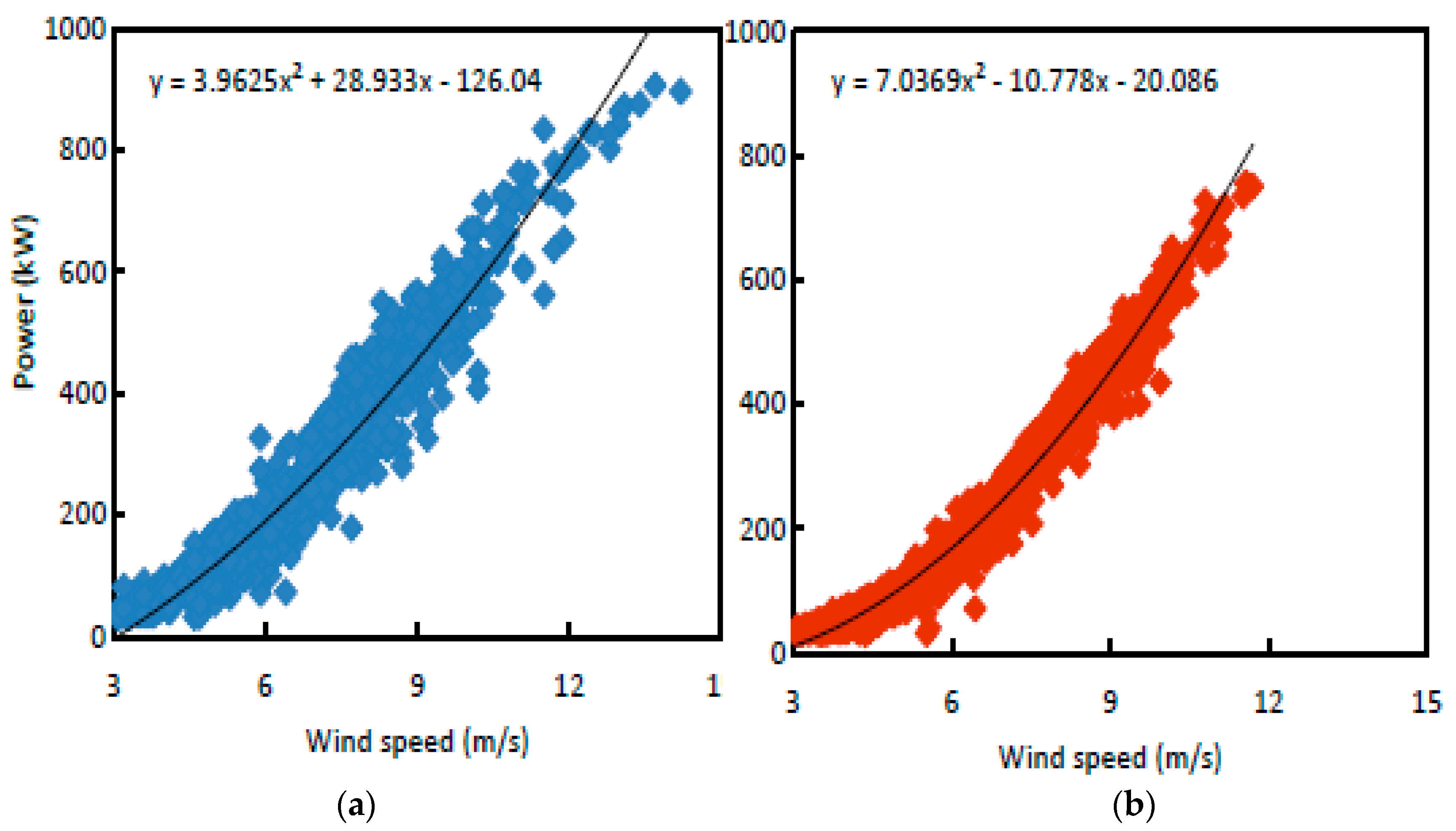
In this case however, coefficients a, b, and c are obtained from approximations of the curve of best fit for the 20% model development dataset using the method of least squares. By using two representative seasons, differences in atmospheric conditions are accounted for. In Figure 4, the wind turbine used in the study for both winter and summer seasons depict a near linear or polynomial relationship when filtered wind speed and power pairs were plotted. The filtered data is the 20% for model development with wind speed less than the cut-in speed and wind power less than 30 kW excluded.
Table 3 shows details of the constants, with correlation coefficients of the APC and the EPC of 0.94 and 0.98 for winter and summer, respectively. The dataset also corroborate earlier inferences that average wind speed is higher during winter than during summer.
In Figure 5, it is observed that the estimation error between the APC and EPC for each of the time steps in the 15-min interval time series reduces considerably when compared to its equivalent TPC. The high R values give credence to the fact that polynomial functions are valid for explaining the relationship between wind speed and wind power for time-series estimation. A limitation (quite similar to that of the TPC) is present, which requires that the EPC be “corrected” at the rated speed. This correction imposes constant wind power production (rated power of the turbine) when the wind speed is between 15 m/s and 25 m/s.
Table 4 provides a statistical summary of the performance of the EPC for the scenarios considered, comparing with that of the TPC with respect to actual power generated. The EPC performed best in Scenario A, with an approximately 3% underestimation of total yield in kWh in winter, while for summer there is an overestimation, also of 3%. The maximum error recorded is an overestimation of 35% during summer for scenario B. This illustrates the sensitivity of the wind turbine to poor weather conditions.
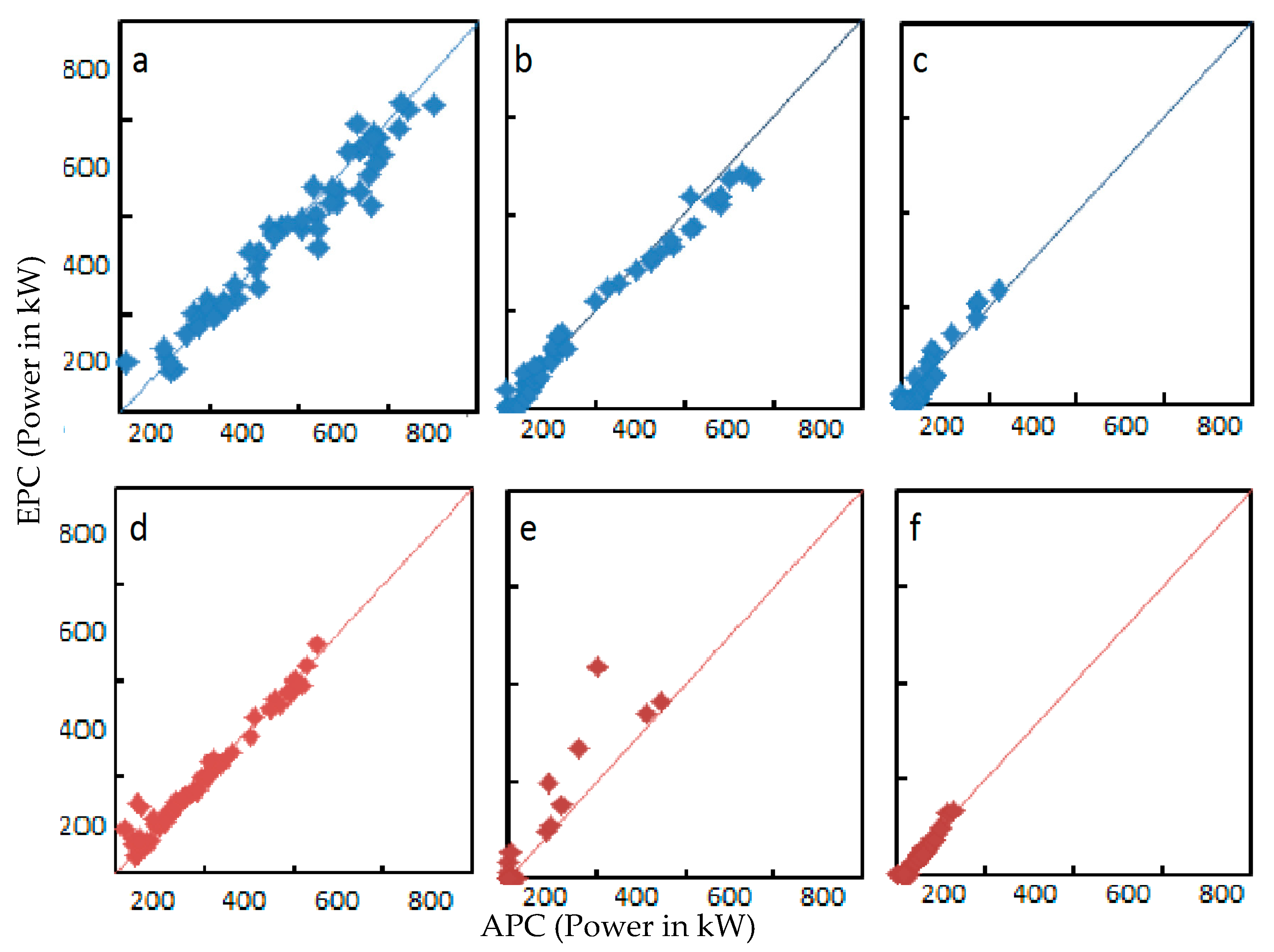
Figure 6 gives a diagrammatic representation of the accuracy and consistency of the EPC (predicted output) relative to the APC (actual values). The degree of alignment of points on the diagonal line indicates the accuracy of the predictions. The performance is satisfactory for all scenarios, although the most accurate predictions appear to be during scenario A, where wind conditions are highly favorable for continued wind turbine operation.
4. Conclusions
Time series of wind turbine performance and energy yield were examined under three different scenarios using two representative seasons (i.e., winter and summer). First, a 1-min interval time series comparison of actual turbine output (APC) and theoretical turbine output (TPC) was considered. The observed data show that wind direction may significantly impact turbine power output; likewise turbine momentum may sustain wind power production despite low wind speed. Knowledge of this effect and its dynamics is very useful for guiding the actions of wind turbine controllers and operators. The 5-min and 15-min interval time series appear more suited for addressing delays in turbine response, developing energy storage systems, energy scheduling, and load management, and bear greater significance in electrical grid quality and stability. All the cases and scenarios considered exhibit relatively large estimation errors both for each time step and for the total energy yield in kWh. These errors are major underestimations of actual power and could directly hinder wind power diffusion and optimization, especially in terms of acceptance, adoption, and commercialization.
An effective power curve (EPC) was proposed based on turbine performance over a given period. The EPC produces fewer estimation errors relative to the TPC when used for estimating power production in the 15-min interval time series. The EPC afforded an easier and more direct estimation of turbine power production, with an estimation error of less than 5% (average value) during “good” wind conditions. Better estimates during good wind conditions offer optimal value in terms of wind power exploitation and harnessing. Generated energy does not have to be disposed-off while energy from alternate sources (non-stochastic/intermittent) can be stored or reserved Energy Storage Systems (ESS). However, under poor wind conditions where the performance of the EPC is less remarkable other strategies may be required in addition. Typically, a change in turbine blade operating conditions such as turbine shut-down or sustaining a certain rotational speed may be more beneficial for accurate estimations. Another strategy can require operator changes to the turbine tip speed ratio (TSR), thus creating a better define estimate. These strategies are however best suited for defined environmental conditions and relatively higher wind speeds (higher mean value but less time-step fluctuations). Importantly, studies on turbine performance during poor wind and wind ramp events would be scaled up in the near future, requiring a combination of approaches (computational fluid dynamic modeling, machine learning, and or support vector mechanism) validated with field observations to increase estimation accuracy. This line of knowledge provides a great motivation for our future studies based on the foundation provided in this study.
Since estimation errors and fluctuations occur irrespective of turbine type, location, and size, an essential step by energy producers would be to create their turbine or wind farm EPC before grid connection. By combining the turbine EPC approach with accurate short-term wind prediction tools such as the ARMA, ARIMA, and exponential smoothing methods, wind power prediction and estimation for very very short term (>5 min) and very short term (10 min–6 h) can be done more accurately. This would foster wind power optimization, positively influence the wind energy market, and improve wind power diffusion. Also, by minimizing estimation errors, policy support for increasing wind power share in energy portfolios may be more easily achieved.
Supplementary Materials
The following are available online at https://www.mdpi.com/1996-1073/11/8/1992/s1, Figure S1: Coefficient of Performance curve profile for the Nordex-N50 wind turbine.
Author Contributions
The study idea, plan and design were conceived by W.Z. and A.T.A. Calculations, analysis and visualizations were carried out by A.T.A. and W.Z., who jointly prepared the manuscript, discussed the results and decided on the final version.
Funding
The first author is a recipient of a research studentship provided by the City University of Hong Kong.
Acknowledgments
The authors would like to thank the Energy Company whose wind turbine data were used for this study. We are also grateful to the anonymous reviewers for their insightful comments, which helped improve the overall quality of this publication.
Conflicts of Interest
The authors declare no conflict of interest.
References
- Negnevitsky, M.; Potter, C.W. Innovative short-term wind generation prediction techniques. In Proceedings of the Power Systems Conference and Exposition, Atlanta, GA, USA, 29 October–1 November 2006; pp. 60–65. [Google Scholar]
- Valentine, S.V. A STEP toward understanding wind power development policy barriers in advanced economies. Renew. Sustain. Energy Rev. 2010, 14, 2796–2807. [Google Scholar] [CrossRef]
- Renani, E.T.; Elias, M.F.M.; Rahim, N.A. Using data-driven approach for wind power prediction: A comparative study. Energy Convers. Manag. 2016, 118, 193–203. [Google Scholar] [CrossRef]
- Bludszuweit, H.; Domínguez-Navarro, J.A.; Llombart, A. Statistical analysis of wind power forecast error. IEEE Trans. Power Syst. 2008, 23, 983–991. [Google Scholar] [CrossRef]
- García-Bustamante, E.; González-Rouco, J.F.; Jiménez, P.A.; Navarro, J.; Montávez, J.P. A comparison of methodologies for monthly wind energy estimation. Wind Energy 2009, 12, 640–659. [Google Scholar] [CrossRef]
- García-Bustamante, E.; González-Rouco, J.F.; Jiménez, P.A.; Navarro, J.; Montávez, J.P. The influence of the Weibull assumption in monthly wind energy estimation. Wind Energy 2008, 11, 483–502. [Google Scholar] [CrossRef]
- Akinsanola, A.A.; Ogunjobi, K.O.; Abolude, A.T.; Sarris, S.C.; Ladipo, K.O. Assessment of wind energy potential for small communities in south-south Nigeria: Case study of Koluama, Bayelsa State. J. Fundam. Renew. Energy Appl. 2017, 7, 1–6. [Google Scholar] [CrossRef]
- Abolude, A.; Zhou, W. A preliminary analysis of wind turbine energy yield. Energy Procedia 2017, 138, 423–428. [Google Scholar] [CrossRef]
- Villanueva, D.; Feijóo, A. Normal-based model for true power curves of wind turbines. IEEE Trans. Sustain. Energy 2016, 7, 1005–1011. [Google Scholar] [CrossRef]
- Kusiak, A. Share data on wind energy. Nature 2016, 529, 19–21. [Google Scholar] [CrossRef] [PubMed]
- Staffell, I.; Green, R. How does wind farm performance decline with age? Renew. Energy 2014, 66, 775–786. [Google Scholar] [CrossRef]
- Li, S.; Wunsch, D.C.; O’Hair, E.A.; Giesselmann, M.G. Using neural networks to estimate wind turbine power generation. IEEE Trans. Energy Convers. 2001, 16, 276–282. [Google Scholar]
- Schlechtingen, M.; Santos, I.F.; Achiche, S. Using data-mining approaches for wind turbine power curve monitoring: A comparative study. IEEE Trans. Sustain. Energy 2013, 4, 671–679. [Google Scholar] [CrossRef]
- Shokrzadeh, S.; Jozani, M.J.; Bibeau, E. Wind turbine power curve modeling using advanced parametric and nonparametric methods. IEEE Trans. Sustain. Energy 2014, 5, 1262–1269. [Google Scholar] [CrossRef]
- Long, H.; Wang, L.; Zhang, Z.; Song, Z.; Xu, J. Data-driven wind turbine power generation performance monitoring. IEEE Trans. Ind. Electron. 2015, 62, 6627–6635. [Google Scholar] [CrossRef]
- Cooney, C.; Byrne, R.; Lyons, W.; O’Rourke, F. Performance characterisation of a commercial-scale wind turbine operating in an urban environment, using real data. Energy Sustain. Dev. 2017, 36, 44–54. [Google Scholar] [CrossRef]
- Lei, M.; Shiyan, L.; Chuanwen, J.; Hongling, L.; Yan, Z. A review on the forecasting of wind speed and generated power. Renew. Sustain. Energy Rev. 2009, 13, 915–920. [Google Scholar] [CrossRef]
- Foley, A.M.; Leahy, P.G.; Marvuglia, A.; McKeogh, E.J. Current methods and advances in forecasting of wind power generation. Renew. Energy 2012, 37, 1–8. [Google Scholar] [CrossRef] [Green Version]
- Riahy, G.H.; Abedi, M. Short term wind speed forecasting for wind turbine applications using linear prediction method. Renew. Energy 2008, 33, 35–41. [Google Scholar] [CrossRef]
- Kavasseri, R.G.; Seetharaman, K. Day-ahead wind speed forecasting using f-ARIMA models. Renew. Energy 2009, 34, 1388–1393. [Google Scholar] [CrossRef]
- Erdem, E.; Shi, J. ARMA based approaches for forecasting the tuple of wind speed and direction. Appl. Energy 2011, 88, 1405–1414. [Google Scholar] [CrossRef]
- Chen, P.; Pedersen, T.; Bak-Jensen, B.; Chen, Z. ARIMA-based time series model of stochastic wind power generation. IEEE Trans. Power Syst. 2010, 25, 667–676. [Google Scholar] [CrossRef]
- Lind, P.G.; Herráez, I.; Wächter, M.; Peinke, J. Fatigue load estimation through a simple stochastic model. Energies 2014, 7, 8279–8293. [Google Scholar] [CrossRef]
- Lind, P.G.; Vera-Tudela, L.; Wächter, M.; Kühn, M.; Peinke, J. Normal Behaviour Models for Wind Turbine Vibrations: Comparison of Neural Networks and a Stochastic Approach. Energies 2017, 10, 1944. [Google Scholar] [CrossRef]
- Simani, S.; Farsoni, S. Fault Diagnosis and Sustainable Control of Wind Turbines: Robust Data-Driven and Model-Based Strategies; Butterworth-Heinemann: Oxford, UK, 2018. [Google Scholar]
- Milan, P.; Wächter, M.; Peinke, J. Stochastic modeling and performance monitoring of wind farm power production. J. Renew. Sustain. Energy 2014, 6, 033119. [Google Scholar] [CrossRef] [Green Version]
- Zanon, A.; De Gennaro, M.; Kühnelt, H. Wind energy harnessing of the NREL 5 MW reference wind turbine in icing conditions under different operational strategies. Renew. Energy 2018, 115, 760–772. [Google Scholar] [CrossRef]
- Doherty, R.; O’Malley, M. A new approach to quantify reserve demand in systems with significant installed wind capacity. IEEE Trans. Power Syst. 2005, 20, 587–595. [Google Scholar] [CrossRef]
- Kaldellis, J.K.; Kavadias, K.A.; Filios, A.E.; Garofallakis, S. Income loss due to wind energy rejected by the Crete island electrical network—The present situation. Appl. Energy 2004, 79, 127–144. [Google Scholar] [CrossRef]
- Fabbri, A.; Roman, T.G.S.; Abbad, J.R.; Quezada, V.M. Assessment of the cost associated with wind generation prediction errors in a liberalized electricity market. IEEE Trans. Power Syst. 2005, 20, 1440–1446. [Google Scholar] [CrossRef]
- Lydia, M.; Kumar, S.S.; Selvakumar, A.I.; Kumar, G.E.P. A comprehensive review on wind turbine power curve modeling techniques. Renew. Sustain. Energy Rev. 2014, 30, 452–460. [Google Scholar] [CrossRef]
- Azad, A.K.; Rasul, M.G.; Yusaf, T. Statistical diagnosis of the Best Weibull methods for wind power assessment for agricultural applications. Energies 2014, 7, 3056–3085. [Google Scholar] [CrossRef]
- Lu, L.; Yang, H.; Burnett, J. Investigation on wind power potential on Hong Kong islands—An analysis of wind power and wind turbine characteristics. Renew. Energy 2002, 27, 1–12. [Google Scholar] [CrossRef]
- Lynn, P.A. Onshore and Offshore Wind Energy: An Introduction; John Wiley & Sons: New York, NY, USA, 2012; 233p, ISBN 9780470976081. [Google Scholar]
- Gao, X.; Yang, H.; Lu, L. Study on offshore wind power potential and wind farm optimization in Hong Kong. Appl. Energy 2014, 130, 519–531. [Google Scholar] [CrossRef]
- Ashtine, M.; Bello, R.; Higuchi, K. Assessment of wind energy potential over Ontario and Great Lakes using the NARR data: 1980–2012. Renew. Sustain. Energy Rev. 2016, 56, 272–282. [Google Scholar] [CrossRef]
- Hansen, K.S.; Barthelmie, R.J.; Jensen, L.E.; Sommer, A. The impact of turbulence intensity and atmospheric stability on power deficits due to wind turbine wakes at Horns Rev wind farm. Wind Energy 2012, 15, 183–196. [Google Scholar] [CrossRef] [Green Version]
- Lubitz, W.D. Impact of ambient turbulence on performance of a small wind turbine. Renew. Energy 2014, 61, 69–73. [Google Scholar] [CrossRef]
- Emeis, S. Current issues in wind energy meteorology. Meteorol. Appl. 2014, 21, 803–819. [Google Scholar] [CrossRef] [Green Version]
- Thapar, V.; Agnihotri, G.; Sethi, V.K. Critical analysis of methods for mathematical modelling of wind turbines. Renew. Energy 2011, 36, 3166–3177. [Google Scholar] [CrossRef]
- Jafarian, M.; Ranjbar, A.M. Fuzzy modeling techniques and artificial neural networks to estimate annual energy output of a wind turbine. Renew. Energy 2010, 35, 2008–2014. [Google Scholar] [CrossRef]
- Carrillo, C.; Montaño, A.O.; Cidrás, J.; Díaz-Dorado, E. Review of power curve modelling for wind turbines. Renew. Sustain. Energy Rev. 2013, 21, 572–581. [Google Scholar] [CrossRef]
Figure 1.
Turbine actual and theoretical power output during scenario A for: 1-min time intervals in (a) winter and (b) summer; 5-min time intervals in (c) winter and (d) summer; and 15-min time intervals in (e) winter and (f) summer, with average wind speed bars inset.
Figure 1.
Turbine actual and theoretical power output during scenario A for: 1-min time intervals in (a) winter and (b) summer; 5-min time intervals in (c) winter and (d) summer; and 15-min time intervals in (e) winter and (f) summer, with average wind speed bars inset.

Figure 2.
Turbine actual and theoretical power output during scenario B for: 1-min time intervals in (a) winter and (b) summer; 5-min time intervals in (c) winter and (d) summer; and 15-min time intervals in (e) winter and (f) summer, with average wind speed bars inset.
Figure 2.
Turbine actual and theoretical power output during scenario B for: 1-min time intervals in (a) winter and (b) summer; 5-min time intervals in (c) winter and (d) summer; and 15-min time intervals in (e) winter and (f) summer, with average wind speed bars inset.

Figure 3.
Turbine actual and theoretical power output during scenario C for: 1-min time intervals in (a) winter and (b) summer; 5-min time intervals in (c) winter and (d) summer; and 15-min time intervals in (e) winter and (f) summer, with average wind speed bars inset.
Figure 3.
Turbine actual and theoretical power output during scenario C for: 1-min time intervals in (a) winter and (b) summer; 5-min time intervals in (c) winter and (d) summer; and 15-min time intervals in (e) winter and (f) summer, with average wind speed bars inset.

Figure 4.
Dataset B observed wind speed and wind power pairs (after filtering) for Nordex N50-800 kW wind turbine in (a) winter and (b) summer.
Figure 4.
Dataset B observed wind speed and wind power pairs (after filtering) for Nordex N50-800 kW wind turbine in (a) winter and (b) summer.

Figure 5.
15-min interval time series turbine APC (actual output) and EPC (predicted output) for: scenario A in (a) winter and (b) summer; scenario B in (c) winter and (d) summer; and scenario C in (e) winter and (f) summer, with average wind speed bars inset.
Figure 5.
15-min interval time series turbine APC (actual output) and EPC (predicted output) for: scenario A in (a) winter and (b) summer; scenario B in (c) winter and (d) summer; and scenario C in (e) winter and (f) summer, with average wind speed bars inset.

Figure 6.
Comparison of 15-min actual output in kW (APC) and modelled output (EPC) in kW for: scenario A in (a) winter and (d) summer; scenario B in (b) winter and (e) summer; and scenario C in (c) winter and (f) summer.
Figure 6.
Comparison of 15-min actual output in kW (APC) and modelled output (EPC) in kW for: scenario A in (a) winter and (d) summer; scenario B in (b) winter and (e) summer; and scenario C in (c) winter and (f) summer.


Table 1.
Literature with evidence of dispersion of actual power curve from the theoretical power curve.
Table 1.
Literature with evidence of dispersion of actual power curve from the theoretical power curve.
| Author | Study Context/Focus | WT 1 Model | Location | Time Interval |
|---|---|---|---|---|
| [9] | WT true power curves | Made AE-61 Bonus 1.3 MW | Galicia, Spain | 10-min |
| [10] | Sharing wind energy data | N.A 2 | N.A | 10-min |
| [11] | Wind farm performance decline with aging | N.A (wind farm) | UK | Hourly |
| [12] | Wind turbine power estimation using Neural network | N.A–500 kW | Texas, US | 10-min |
| [13] | Data-mining for WTPCs 3 | N.A–2 MW | Germany | 10-min |
| [14] | WT power curve modeling | Vestas V82–1650 kW | Canada | Hourly |
| [15] | WT power generation performance | N.A (Wind farm) | US | 10 s |
| [16] | Wind turbine performance in urban environment | Vestas V52–850 kW | Ireland | 10-min |
1 WT: Wind Turbine; 2 N.A: Not Available; 3 WTPC: Wind Turbine Power Curve.
Table 2.
Descriptive statistics of observed wind speed distribution (units in m/s).
| Scenario | Winter | Summer | ||||
|---|---|---|---|---|---|---|
| Scenario A | 1-min | 5-min | 15-min | 1-min | 5-min | 15-min |
| Mean | 8.61 | 8.29 | 7.73 | 7.46 | 7.54 | 6.22 |
| Std. dev. | 0.78 | 1.13 | 1.69 | 1.36 | 1.28 | 1.44 |
| Range | 3.30 | 4.88 | 6.00 | 5.83 | 4.94 | 5.47 |
| Scenario B | ||||||
| Mean | 4.15 | 6.37 | 4.87 | 2.87 | 4.14 | 2.46 |
| Std. dev. | 1.57 | 1.46 | 2.25 | 1.10 | 1.77 | 1.95 |
| Range | 5.30 | 6.78 | 9.20 | 4.65 | 5.82 | 8.74 |
| Scenario C | ||||||
| Mean | 4.78 | 5.04 | 3.27 | 5.30 | 3.66 | 3.50 |
| Std. dev. | 1.46 | 1.79 | 1.16 | 1.63 | 2.24 | 0.87 |
| Range | 6.10 | 6.52 | 4.70 | 7.00 | 5.82 | 4.05 |
Table 3.
Details of constants and correlation coefficients for the effective power curve.
| Constant | Winter | Summer |
|---|---|---|
| a | 3.96 | 7.04 |
| b | 28.94 | −10.78 |
| c | −126.04 | −20.09 |
| R | 0.9713 | 0.9880 |
Table 4.
Statistical performance of the effective power curve.
| Error | Winter | Summer | |||||
|---|---|---|---|---|---|---|---|
| Scenario A | Scenario B | Scenario C | Scenario A | Scenario B | Scenario C | ||
| MAE | EPC | 31.10 | 19.80 | 19.01 | 13.14 | 22.44 | 11.00 |
| - | TPC | 103.62 | 76.95 | 20.87 | 64.88 | 9.90 | 24.92 |
| MSE | EPC | 6.45 | 5.05 | 4.68 | 3.49 | 6.13 | 2.79 |
| - | TPC | 10.84 | 10.63 | 5.53 | 8.54 | 4.95 | 5.20 |
| RMSE | EPC | 41.56 | 25.55 | 21.86 | 12.10 | 37.55 | 7.80 |
| - | TPC | 117.54 | 113.00 | 30.56 | 72.91 | 24.55 | 27.02 |
© 2018 by the authors. Licensee MDPI, Basel, Switzerland. This article is an open access article distributed under the terms and conditions of the Creative Commons Attribution (CC BY) license (http://creativecommons.org/licenses/by/4.0/).
Share and Cite
MDPI and ACS Style
Abolude, A.T.; Zhou, W. Assessment and Performance Evaluation of a Wind Turbine Power Output. Energies 2018, 11, 1992. https://doi.org/10.3390/en11081992
AMA Style
Abolude AT, Zhou W. Assessment and Performance Evaluation of a Wind Turbine Power Output. Energies. 2018; 11(8):1992. https://doi.org/10.3390/en11081992
Chicago/Turabian StyleAbolude, Akintayo Temiloluwa, and Wen Zhou. 2018. "Assessment and Performance Evaluation of a Wind Turbine Power Output" Energies 11, no. 8: 1992. https://doi.org/10.3390/en11081992
Note that from the first issue of 2016, this journal uses article numbers instead of page numbers. See further details here.