Quantifying Drought Propagation from Soil Moisture to Vegetation Dynamics Using a Newly Developed Ecohydrological Land Reanalysis

Meteorological Research Institute, Japan Meteorological Agency, Tsukuba 305-0052, Japan
Remote Sens. 2018, 10(8), 1197; https://doi.org/10.3390/rs10081197
Submission received: 23 June 2018
/
Revised: 19 July 2018
/
Accepted: 27 July 2018
/
Published: 30 July 2018
(This article belongs to the Special Issue Assimilation of Remote Sensing Data into Earth System Models)
Abstract
:Despite the importance of the interaction between soil moisture and vegetation dynamics to understand the complex nature of drought, few land reanalyses explicitly simulate vegetation growth and senescence. In this study, I provide a new land reanalysis which explicitly simulates the interaction between sub-surface soil moisture and vegetation dynamics by the sequential assimilation of satellite microwave brightness temperature observations into a land surface model (LSM). Assimilating satellite microwave brightness temperature observations improves the skill of a LSM to simultaneously simulate soil moisture and the seasonal cycle of leaf area index (LAI). By analyzing soil moisture and LAI simulated by this new land reanalysis, I identify the drought events which significantly damage LAI on the climatological day-of-year of the LAI’s seasonal peak and quantify drought propagation from soil moisture to LAI in the global snow-free region. On average, soil moisture in the shallow soil layers (0–0.45 m) quickly recovers from the drought condition before the climatological day-of-year of the LAI’s seasonal peak while soil moisture in the deeper soil layer (1.05–2.05 m) and LAI recover from the drought condition approximately 100 days after the climatological day-of-year of the LAI’s seasonal peak.

1. Introduction
Drought is one of the costliest natural disasters in the world [1], so mitigating negative impacts of catastrophic drought events on society is a grand challenge for hydrological researchers and practitioners. Drought monitoring and prediction capabilities contribute to building resilience against severe drought events. Many previous studies have provided the important contributions to drought monitoring [2,3,4], and drought prediction [5,6,7]. In those literatures, precipitation, soil moisture, and vegetation condition were recognized as the key variables to be observed and/or simulated for drought monitoring and prediction.
Understanding the complex nature of drought from historical drought events is strongly needed to improve drought monitoring and early warning and help decision makers consider the adaptation plan against severe drought events. Drought is a complicated multi-spatiotemporal phenomenon and an integrated process which has meteorological, hydrological, and ecological aspects. According to the conceptual model proposed by Wilhite and Glantz [8], extreme climate conditions such as precipitation deficiency and high temperature induce soil water deficiency which causes plant water stress and agricultural drought. Then, streamflow and groundwater level respond to soil water deficiency, which causes hydrological drought. Soil moisture has an important role in this drought propagation since it controls both agricultural and hydrological aspects of drought. Quantifying the drought propagation is important to deliver the effective information of the drought progress to decision makers in a wide variety of sectors and has been intensively investigated. Sawada et al. [9] found that hydrological drought quantified by river discharge and groundwater level lasted longer than agricultural drought quantified by vegetation dynamics in Medjerda river basin, Tunisia. Sepulcre-Canto et al. [10] developed a drought indicator in Europe considering the drought propagation from soil moisture deficits to crop failures. Akarsh and Mishra [11] analyzed the drought propagation from soil moisture in shallow soil layers to vegetation condition in India. These previous studies indicated that the interaction between soil moisture and vegetation dynamics is important to understand the drought propagation. However, published knowledge is limited to regional applications and the holistic view of the drought propagation from soil moisture to vegetation dynamics has yet to be obtained.
To identify and quantify the drought propagation, land reanalysis is useful since it provides spatially and temporally homogeneous terrestrial water cycle data. Land reanalysis is generated by driving a land surface model (LSM) with meteorological forcings from atmospheric reanalysis with adjustments using in situ observation networks. For example, the Global Land Data Assimilation System (GLDAS) [12] provides land surface variables such as soil moisture globally from 1948 to present by driving multiple LSMs. MERRA-Land [13] provides global estimates of soil moisture, heat fluxes, snow, and runoff from 1979 to present as a part of the Modern-Era Retrospective Analysis for Research and Applications (MERRA) reanalysis. ERA-Interim/Land [14] is generated by a single 32-year (1979–2010) simulation of the European Centre for the Medium Range Weather Forecasts (ECMWF) land surface model driven by meteorological forcings from the ERA-Interim atmospheric reanalysis. These land reanalysis datasets were widely used for drought identification and quantification [11,15,16,17,18,19,20].
However, there are limitations in the existing land reanalysis datasets for the quantification of the drought propagation. First, few land reanalyses explicitly simulate vegetation growth and senescence. The interaction between soil moisture and vegetation dynamics is not currently considered by the LSMs which are used to generate global land reanalysis datasets. The decline of vegetation activity due to drought cannot be identified and quantified by the existing global land reanalysis datasets although the ecohydrological process is important in the drought propagation.
Second, few satellite observations are assimilated into LSMs in the current global land reanalyses. There are important satellite observations which can improve the simulation of a LSM. For example, passive and active microwave remote sensing provides the all-sky observation of land surface soil moisture, temperature, and vegetation water content [21,22,23,24,25,26,27]. Although many previous studies have developed Land Data Assimilation Systems (LDASs) to assimilate these satellite microwave observations into a LSM [28,29,30,31,32,33,34,35] and some previous studies have successfully monitored regional drought events using LDASs [7,36], they have yet to be fully applied to generate land reanalysis for the quantification of the drought propagation.
There are several LDASs which can accurately simulate both soil moisture and vegetation dynamics. Barbu et al. [37] assimilated satellite-observed surface soil moisture and leaf area index (LAI) jointly into a LSM which can simultaneously calculate soil moisture and vegetation dynamics. Liu et al. [38] assimilated both active and passive microwave observations into a LSM and demonstrated that data assimilation can improve the simulation of soil moisture and biomass. Sawada and Koike [39] and Sawada et al. [40] developed the Coupled Land and Vegetation Data Assimilation System (CLVDAS) which can improve the skill of a LSM to simulate both soil moisture and vegetation dynamics by assimilating satellite microwave brightness temperature observations. These ecohydrological LDASs are the promising tools to monitor the drought propagation considering the interaction between soil moisture and vegetation dynamics. However, the skill of the ecohydrological LDASs to simultaneously estimate surface soil moisture, sub-surface soil moisture, and vegetation dynamics has yet to be fully validated on continental and global scales.
This study aims to quantify the drought propagation from soil moisture to vegetation dynamics in the global snow-free region. First, I develop a verified land reanalysis, which includes both soil moisture and vegetation condition, by driving CLVDAS. Then, I obtain the holistic view of the integrated drought propagation from soil moisture deficits to vegetation degradation using soil moisture and LAI simulated by the new land reanalysis.
2. Materials and Methods
2.1. Data and Study Area
As observed meteorological forcings, the GLDAS v2.1 data [12,41] were used. GLDAS provides the complete set of meteorological forcings which are needed to run LSMs. The meteorological forcings used in this study were surface pressure, precipitation, surface air temperature, relative humidity, incoming solar radiation, incoming longwave radiation, and wind speed. The horizontal resolution is 0.25 degree. The temporal resolution is 3-hourly and the data were linearly interpolated into hourly data since the time step of the LSM used in this study is set to 1 h.
As microwave brightness temperature observation, the Advanced Microwave Scanning Radiometer for Earth Observing System (AMSR-E) L3 product [42] was used. Brightness temperature observations at 6.925 and 10.25 GHz were used for data assimilation. Both horizontally and vertically polarized observations were used. I used only night scene data since the effect of surface temperature errors on the estimation of microwave brightness temperature is small at night [43]. The native horizontal resolution of the L3 product is 0.1 degree and the data were resampled to 0.25 degree by box averaging to match them to the resolution of the GLDAS meteorological forcings and the LSM. The temporal resolution is approximately 2-daily.
The International Satellite Land Surface Climatology Project 2 soil data [44] were used to derive soil texture. The Food and Agricultural Organization global dataset [45] was used to obtain the parameters for the water retention curve.
The Global Land Surface Satellite LAI (GLASS LAI) product [46] was used to evaluate the skill of the land reanalysis to simulate phenology. The GLASS LAI was generated from MODerate resolution Imaging Spectroradiometer (MODIS) visible and infrared observations [47]. Xiao et al. [46] reported that GLASS LAI could reproduce field-measured LAI with the accuracy of R2 = 0.87 and RMSE = 0.64 [m2/m2]. The native horizontal resolution of the GLASS LAI product is 1 km and I resampled it into 0.25 degree by box averaging. The temporal resolution is 8-daily and I generated the monthly data.
The European Space Agency Climate Change Initiative Soil Moisture (ESA CCI SM) v3.2 product [48,49,50] was used to evaluate the skill of the land reanalysis to simulate surface soil moisture. This product was generated by blending many existing satellite-observed soil moisture products. The combined passive and active microwave products were used. Although Dorigo et al. [48] reported that the correlation coefficient between this product and in situ surface soil moisture observations is approximately 0.6 on average, significantly low correlations are also reported in some in situ observation sites. The horizontal resolution of the ESA CCI SM is 0.25 degree and the temporal resolution is approximately 2-daily.
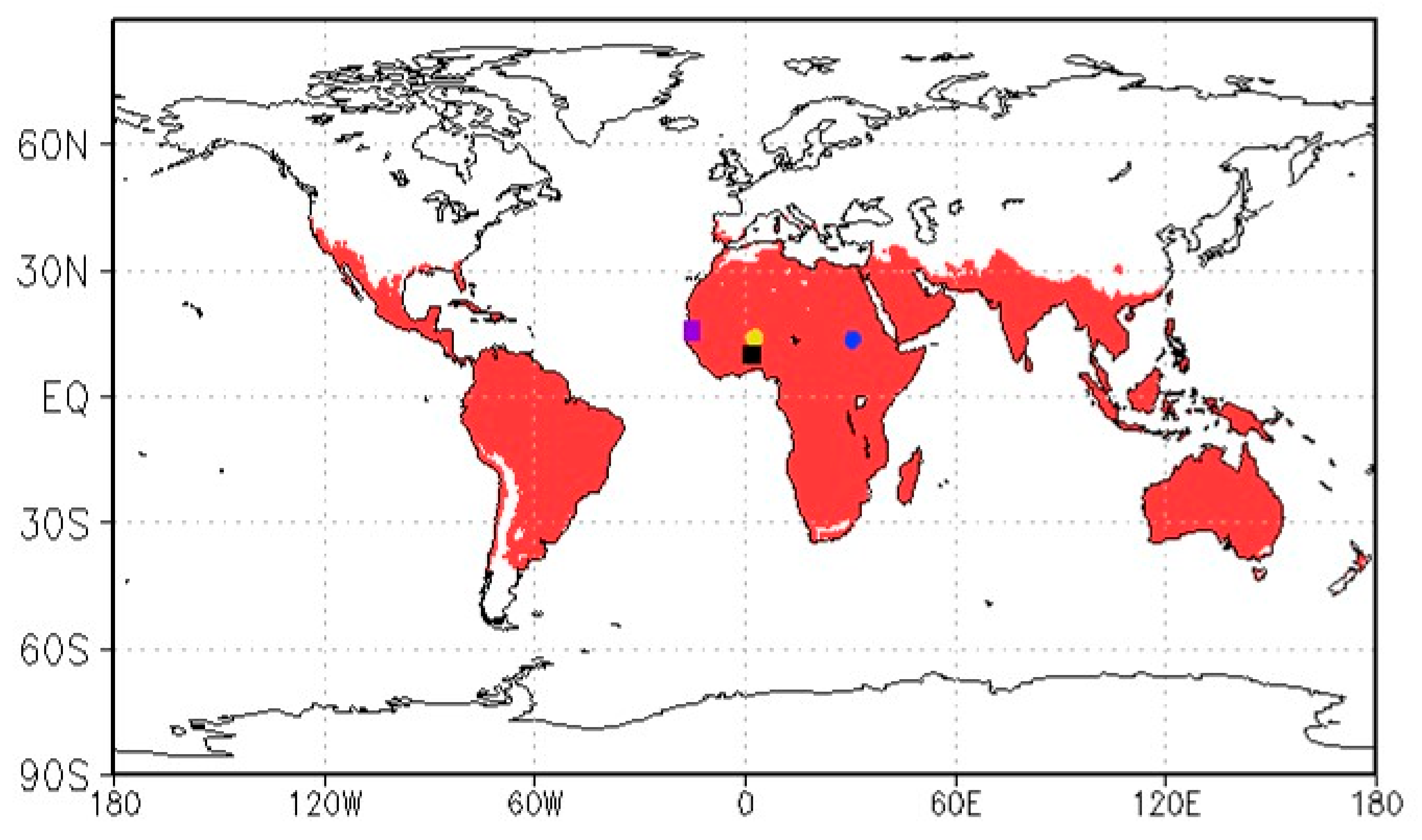
To evaluate the skill of the land reanalysis to simulate soil moisture from surface to 2m depth, I used the in situ soil moisture observations archived at International Soil Moisture Network (ISMN) [51]. I used the network of the African Monsoon Multidisciplinary Analysis—Coupling the Tropical Atmosphere and the Hydrological Cycle (AMMA-CATCH) [52], CARBOAFRICA [53], and Dahra [54]. The land cover of the AMMA-CATCH Belefoungou site is crop and the land cover of the other sites is semi-arid savanna. The annual maximum LAIs in Dahra, CARBOAFRICA, AMMA-CATCH Belefoungou and Tondikiboro are approximately 1.5, 0.6, 2.5, and 0.6, respectively. Figure 1 shows the locations of the in situ soil moisture observation sites. I chose these sites because they provided both surface and subsurface (more than 1 m depth) in situ soil moisture observations with the sufficient observation periods. In addition, as mentioned below, I did not provide the land reanalysis in the pixels in which there is snowfall from 2003 to 2010. These criteria excluded many in situ soil moisture observations in ISMN. The native temporal resolutions of the point-scale observations were resampled to daily. Although the in situ soil moisture observations provide hourly data, here I focused on the daily-scale soil moisture dynamics since soil moisture dynamics in an hourly scale is not important for the application to drought analysis. In addition, the skill to simulate the hourly-scale soil moisture dynamics may be strongly degraded by the bias of the timing of precipitation in the GLDAS data, which cannot be corrected by the LDAS used in this study.
The Emergency Events Database (EM-DAT: http://www.emdat.de) was used as reference data of historical drought events. The EM-DAT provides information on historic natural and technological disasters reported by different institutions across the world. Please note that the database may not include all disasters and the reported damages may sometimes be biased.
The study area was the global snow-free region (Figure 1). I identified the snow-free region using the GLDAS snowfall data. There are two reasons why I focused only on the snow-free region. First, snowmelt may have an important role in the drought propagation in some regions. The drought propagation may be more complicated in snowfall regions than in snow-free regions. In snow-free regions, I can focus only on the interaction between soil moisture and vegetation dynamics to quantify the drought propagation. Second, the performance of my LDAS (see Section 2.2) may be degraded by snow because snow accumulation makes it difficult to simulate microwave radiative transfer. The tau-omega model of the radiative transfer model (RTM) (Equation (9) in Section S2 of the Supplementary Materials) does not currently consider the effect of snow accumulation on microwave radiative transfer. Considering the effect of snow accumulation in the RTM may bring additional errors in the land reanalysis, which was avoided in this study. Please note that the study area includes the arid and semi-arid area in which the effects of vegetation on microwave signals are small so that I can evaluate the impact of the data assimilation on the simulation of surface soil moisture.
2.2. Coupled Land and Vegetation Data Assimilation System (CLVDAS)
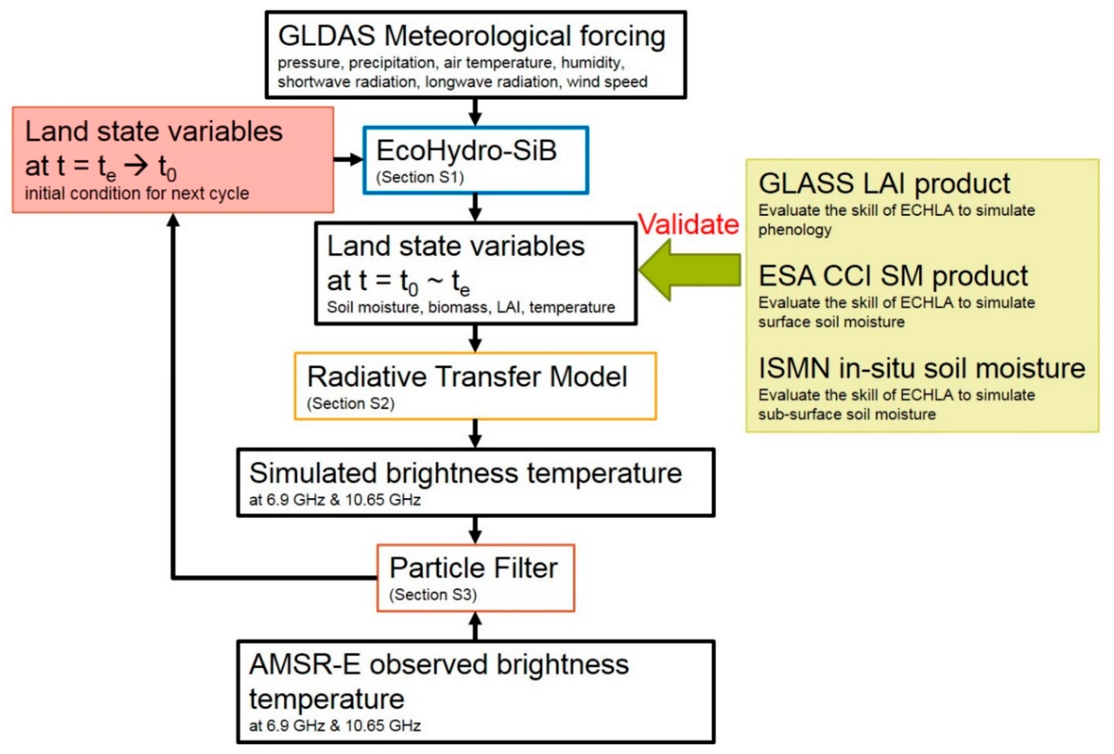
CLVDAS [39,40] has been developed to improve the skill of a LSM to simultaneously simulate soil moisture and vegetation dynamics. The modules of CLVDAS include a LSM, a microwave Radiative Transfer Model (RTM), and a particle filtering (PF) data assimilation system. The LSM of CLVDAS is EcoHydro-SiB, which can simultaneously simulate surface soil moisture, sub-surface soil moisture, and vegetation dynamics (see Section S1 of the Supplementary Materials). EcoHydro-SiB can explicitly simulate vegetation growth and senescence. The RTM of CLVDAS can estimate microwave emissivity on land (see Section S2 of the Supplementary Materials). Microwave brightness temperature at C- and X-bands is sensitive to both surface soil moisture and vegetation water content [23] and insensitive to atmospheric condition. Therefore, the RTM can estimate satellite level microwave brightness temperature from surface soil moisture, surface soil temperature, and vegetation water content simulated by EcoHydro-SiB. The PF can assimilate satellite microwave brightness temperature observations into the LSM and improve the skill of the LSM to simulate their state variables (see Section S3 of the Supplementary Materials). The detailed description of the CLVDAS is not included in this main manuscript and can be found in the Supplementary Materials since the description of all CLVDAS’s modules has already been published. Please refer to previous papers [9,39,40] for the complete description of CLVDAS (i.e., the LSM, the RTM, and the PF data assimilation system) and its parameter variables. References of the Supplementary Materials are also useful to understand the LSM, the RTM, and the PF data assimilation system.
2.3. ECoHydrological Land reAnalysis (ECHLA)
I generated a new land reanalysis dataset, called the ECoHydrological Land reAnalysis (ECHLA), by driving CLVDAS. First, I run EcoHydro-SiB without data assimilation (the open loop (OL) experiment). Initial conditions are 80-year spun-up results of the OL experiment. Second, comparing simulated brightness temperature at 6.9 GHz and 10.65 GHz by the RTM with observed brightness temperature by AMSR-E from 2004 to 2006, I optimized the surface soil roughness parameter of the RTM (rms height: see a previous paper [55]) in each pixel. Although there is another soil roughness parameter, correlation length, in the RTM, I did not optimize it in this study. This is because the combination of large rms height and large correlation length has a similar effect to the combination of small rms height and small correlation length so that it is practically difficult to optimize both of soil roughness parameters simultaneously [39]. The optimization was implemented using the Shuffled Complex Evolution method (SCE-UA) [56]. The parameter optimization method in CLVDAS was described previously [39]. Third, I run EcoHydro-SiB with the assimilation of the AMSR-E observed brightness temperature observations by the PF (the DA experiment). The output of the DA experiment is the dataset of ECHLA.
The horizontal resolution of ECHLA was set to 0.25 degree. The depth of the first soil layer was set to 0.05 m and the depths of the other soil layers were set to 0.1 m. The total soil depth was set to 2.05 m since the previous studies revealed that most of root biomass was distributed from 0 to 2 m depth soil [57]. The temporal resolution of EcoHydro-SiB was set to hourly and I analyzed the daily data.
The observation errors for , , , and are set to 9.9 K, 14 K, 8.3 K, and 13 K, respectively ( is the vertically polarized brightness temperature at 6.9 GHz, for instance). It is generally difficult to objectively determine the observation errors especially for satellite brightness temperature observations [58]. In this study, these variables are set to the mean root-mean-square differences between observed brightness temperature and simulated brightness temperature by the OL experiment averaged in all pixels of the study area. I assumed that the observation errors are uncorrelated. The duration of the data assimilation window was set to 5 days so that past 5 days’ and present observations were assimilated to adjust the model state at the present time. The ensemble size was set to 100 and the ensemble mean was used for the drought identification and quantification.
Figure 2 summarizes production steps of ECHLA. The LSM, EcoHydro-SiB, estimated land state variables for 5 days (from t0 to te in Figure 2) using GLDAS meteorological forcing data. Using the simulated land state variables, such as surface soil moisture, LAI, and temperature, the RTM estimated brightness temperatures at 6.9 GHz and 10.65 GHz from t0 to te. Then, the PF adjusted the land state variables at the end of the data assimilation window (te) by comparing simulated and AMSR-E observed brightness temperatures from t0 to te. The PF assimilated all available observations in the assimilation window. All state variables (i.e., soil moisture in all soil columns, biomass pools, and temperature) were adjusted. The adjusted biomass pools included the leaf, stem, and root biomass and LAI was also updated by calculating it from the adjusted leaf biomass (see also the Supplementary Materials). Since all state variables raised above are included in particles, they are updated by the PF process although they are not directly observed. The adjusted land state variables were used for the initial condition of the next data assimilation cycle.
The study period was set to 2003–2010, which is nearly identical to the period of the AMSR-E operational observation. Although the study period was set to the short duration in this first trial of generating the new land reanalysis, CLVDAS and the existing satellite observation missions have a potential to extend the period (see Section 4.2).
2.4. Drought Identification and Quantification
I identified and quantified the drought propagation using soil moisture and LAI of ECHLA. The drought index used in this study was the Standardized Anomaly (SA) [9,59]:
where is the SA at time t, x(t) is soil moisture or LAI, is the temporal mean of x, and is the standard deviation of x. To calculate (1), I used daily data. For instance, SA of LAI on 1 January 2004 is calculated by the mean and standard deviation of LAI on January 1 in each year (i.e., from 2003 to 2010).
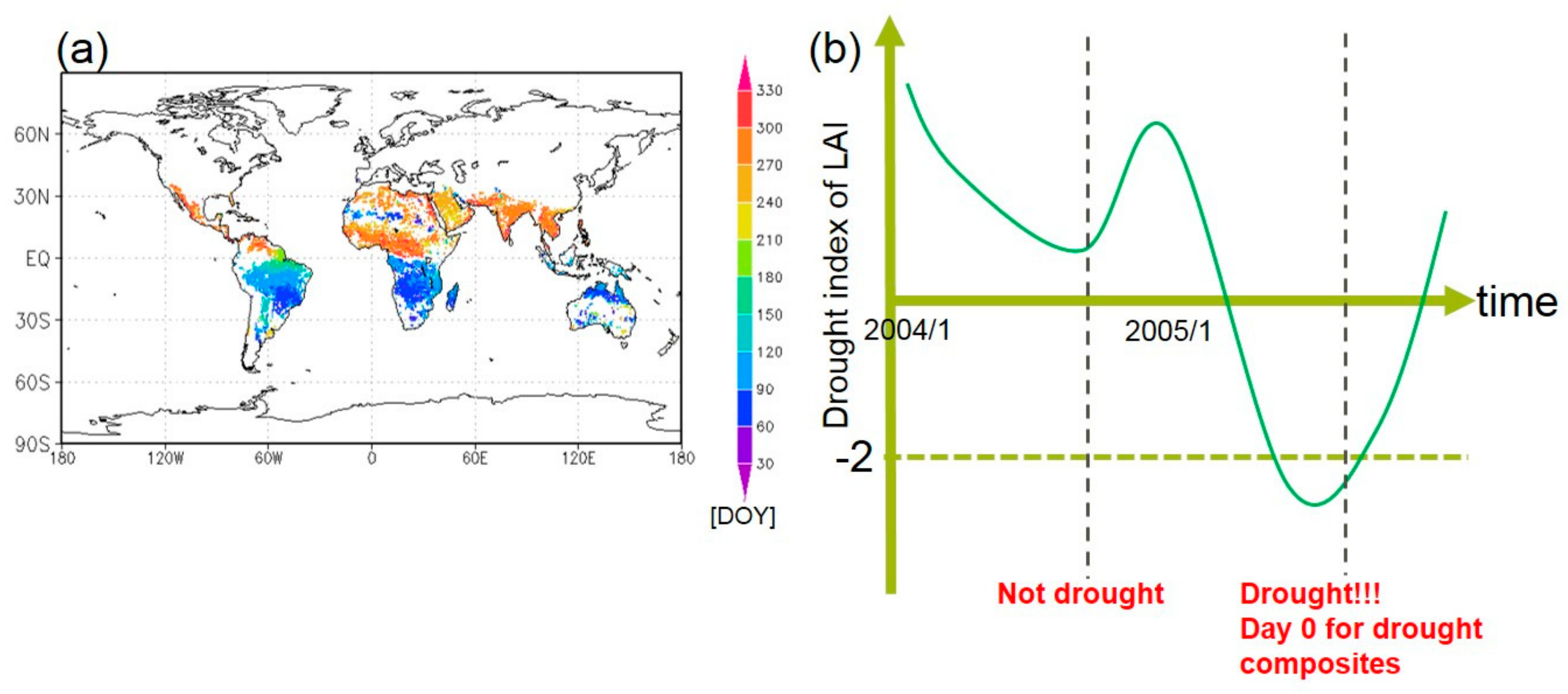
In this paper, I identified drought events using the time series of the SA of LAI. I focused on the vegetation degradation on the day of the seasonal peak as an indicator of drought because it is strongly related to the degradation of the agricultural activities. First, I analyzed the time series of LAI in each pixel using the TIMESAT software [60] and calculated the timing of the LAI’s seasonal peak. TIMESAT can fit the time series of LAI to a polynomial and analytically obtain the timing of the peak of a fitted polynomial. I obtained the climatological day-of-year of the LAI’s seasonal peak averaged from 2003 to 2010 (Figure 3a).
Then, I evaluated the SA of LAI on the climatological day-of-year of the LAI’s seasonal peak every year in each pixel to identify drought events. The threshold of the LAI SA to identify drought events was set to −2.0. This threshold of SA is often used as “extremely dry” in the literature (e.g., [59]). If the LAI SA is less than −2.0 on the climatological day-of-year of the LAI’s seasonal peak, I considered that the drought event occurred (Figure 3b). The 2-year time series of the SAs of LAI, surface soil moisture at 0–0.05 [m] depth (called surface), soil moisture averaged from 0.05 to 0.45 [m] (root 1), soil moisture averaged from 0.45 to 1.05 [m] (root2), and soil moisture averaged from 1.05 to 2.05 [m] (deep) in the identified drought events were extracted. For instance, in the pixel whose climatological day-of-year of the LAI’s seasonal peak is 1 September, I evaluated the SA of LAI on 1 September every year. I found that the SA of LAI was less than −2 on 1 September 2005 (Figure 3b) so that I extract the time series from 1 September 2004 to 1 September 2006 in order to calculate the statistics of the drought event (see below). Please note that I did not assume that the drought event lasted whole two years. I calculated intensity as a minimum value of the SA in each drought event, duration as a length of each drought event when the SA is less than −1.0 and start and end dates of each drought event as timing when the SA goes below and above −1.0, respectively. This threshold of SA (−1.0) is often used as “moderately dry” in the literature (e.g., [59]). If there are multiple drought events when the SA is less than −1.0 during the extracted 2-year period, I used the event which has the longest duration.
3. Results
3.1. Validation of ECHLA
In this subsection, I evaluated the performance of ECHLA to accurately reproduce soil moisture and LAI in the global snow-free region. The correlation coefficient, root-mean-square-error (RMSE), and unbiased RMSE (ubRMSE) were used as metrics.
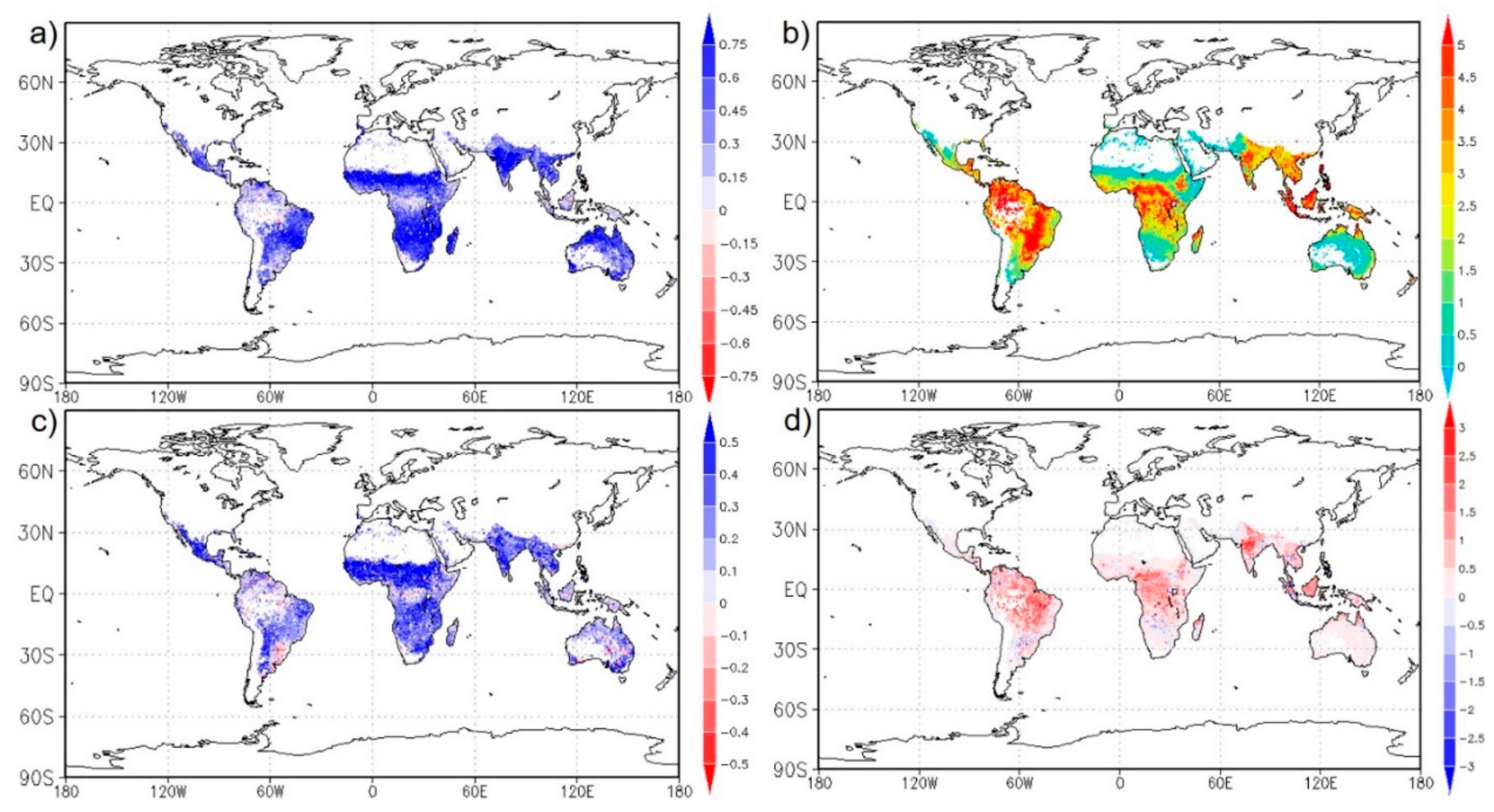
Figure 4 shows the performance of ECHLA to reproduce the optically observed LAI product (GLASS LAI). Both GLASS LAI and ECHLA LAI are temporally resampled to the monthly data. The correlation coefficients between ECHLA LAI and GLASS LAI in most pixels are higher than 0.6 (Figure 4a) so that ECHLA can accurately reproduce the seasonal cycle of LAI. The small correlations can be found in the rainforest regions. Data assimilation greatly contributes to the high performance of ECHLA to reproduce phenology. Figure 4c shows the difference of correlation coefficients against GLASS LAI between the DA experiment and the OL experiment (see Section 3.2). Assimilating microwave brightness temperature observations significantly increases correlation coefficients. However, ECHLA has large RMSEs against GLASS LAI in many regions (Figure 4b) and data assimilation increases them (Figure 4d). Although the absolute value of the optically observed LAI cannot be reliable and directly compared with the model estimation [61] (see also Section 4.1), there may be limitations in the parameterizations to relate LAI to microwave signals.
Figure 5 shows the performance of ECHLA to reproduce the satellite observed surface soil moisture product (ESA CCI). ECHLA surface soil moisture is positively correlated with ESA CCI surface soil moisture in most pixels (Figure 5a). Data assimilation has no significant impacts on correlation coefficients (Figure 5c). Although ECHLA has large RMSEs (≥0.1 m3/m3) against ESA CCI in many regions (Figure 5b), data assimilation generally decreases RMSEs in many pixels (Figure 5d). The improvement of simulating surface soil moisture by data assimilation can be found in Sahel, South Africa, and North Australia. The performance is degraded by data assimilation in the moderately and densely vegetated area such as Ethiopia, South East Asia, and south Amazon (see also Section 4.1).
Table 1, Table 2, Table 3 and Table 4 show the performance of ECHLA to reproduce the in-situ observed soil moisture at the depths of 0–2 m. In all four in situ observation sites, data assimilation improves RMSE and ubRMSE of the surface soil moisture simulation. In the DAHRA site of West Africa, data assimilation decreases RMSEs and increases correlation coefficients against in situ sub-surface soil moisture observations (Table 1). In this site, data assimilation successfully improves the simulation of sub-surface soil moisture, which is not directly observed by the satellite, by inversely estimating sub-surface soil moisture from surface soil moisture and vegetation dynamics (see Section S3 and [40]). The simulation of sub-surface soil moisture is improved only by removing biases so that no significant improvement of ubRMSE can be found. The improvement of the sub-surface soil moisture simulation by data assimilation can also be found in the CARBO AFRICA site of East Africa (Table 2) although the skill of simulating deep-zone (≥1.5 m) soil moisture is degraded when the correlation coefficient is evaluated. The improvement of the skill to simulate sub-surface soil moisture cannot be found in the AMMA-CATCH sites of the Sahel region although data assimilation reduces RMSE and ubRMSE for surface soil moisture (Table 3 and Table 4; see also Section 4.1)
3.2. Identification and Quantification of the Drought Propagation
In this subsection, I identified and quantified the drought propagation using simulated soil moisture and LAI by ECHLA. By the method described in Section 2.4, I identified the drought events. By analyzing the time series of the soil moisture SAs and the LAI SAs in all identified drought events, I present the holistic view of the integrated drought propagation from soil moisture deficits to vegetation degradation.
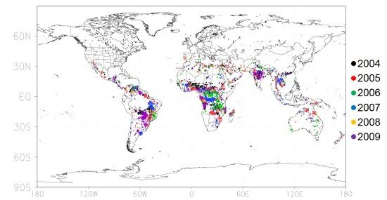
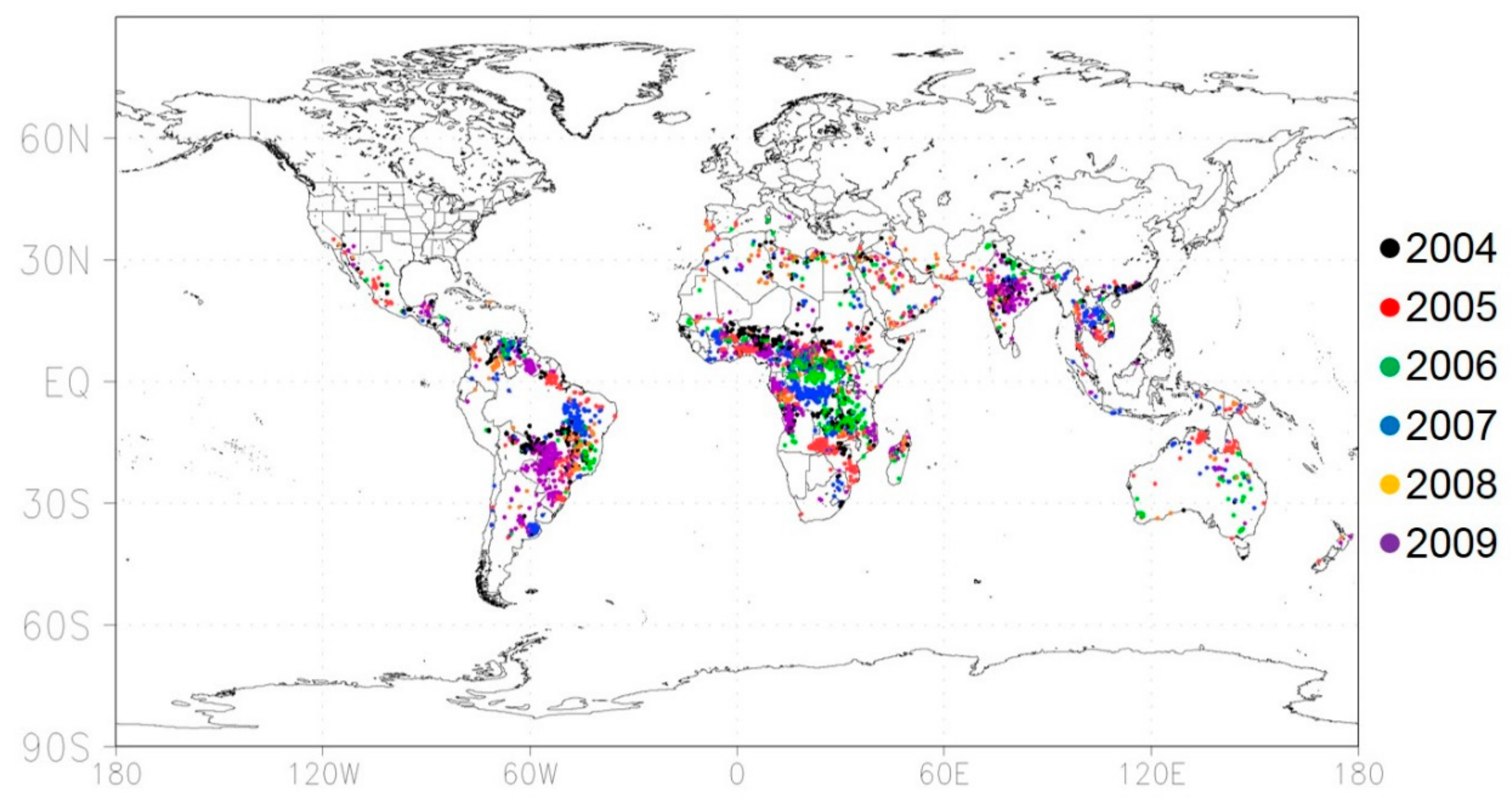
In Figure 6, each dot shows the location of the identified drought event. The color of dots shows the year when the identified drought event occurred. In each dot, the LAI SA is less than −2.0 on the climatological day-of-year of the LAI’s seasonal peak (Figure 3a) in the year shown by the color of the dot. The 3499 drought events (pixels) from 2004 to 2009 are identified.
The identified drought events include the several major droughts listed in EM-DAT such as Brazil in 2005 and 2007, Paraguay in 2009, Zambia in 2005, Ethiopia in 2005, India in 2009, and Thailand in 2005 (Figure 6). ECHLA has the potential to provide the catalog of the historical drought events. However, Figure 6 shows many drought events which are not listed in EM-DAT. For example, there are many dots in the Sahel region although few droughts are reported in EM-DAT there from 2004 to 2009. This is mainly because the study period is too short to obtain enough data to identify the extreme drought events and I incorrectly recognize the relatively small declines of LAI as extremely dry events. In addition, there are many droughts which are listed in EM-DAT but not included in my drought catalog based on ECHLA because the criteria of the drought identification (i.e., the LAI SA is less than −2.0 on the climatological day-of-year of the LAI’s seasonal peak) are strict.
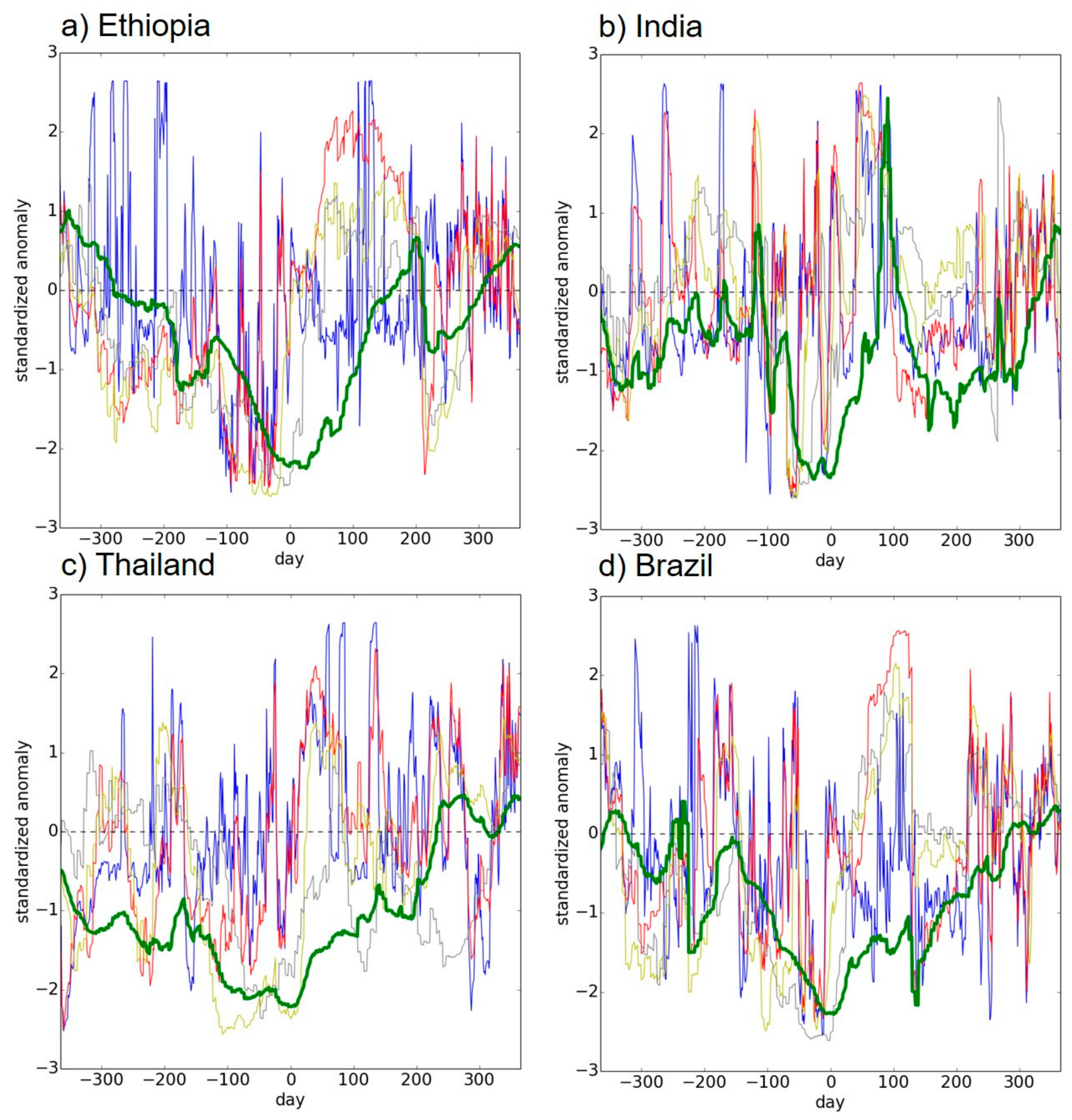
Figure 7 shows the time series of the SAs of LAI, surface soil moisture at 0–0.05 m depth (called surface), soil moisture averaged from 0.05 to 0.45 m depth (root 1), soil moisture averaged from 0.45 to 1.05 m depth (root 2), and soil moisture averaged from 1.05 to 2.05 m depth (deep) in the selected drought events. In each drought event, I set the climatological day-of-year of the LAI’s seasonal peak to day 0 and show the time series of the SAs over 2 years (from day −365 to day +365; see also Figure 3b). In all four drought events shown in Figure 7, the LAI SA has its minimum value on around day 0, which is less than −2.0, due to the criteria to identify the drought events. However, the processes of the decline and recovery of the LAI SA are different in the different drought events. In addition, there is the diversity of the progress of the soil moisture SAs among drought events.
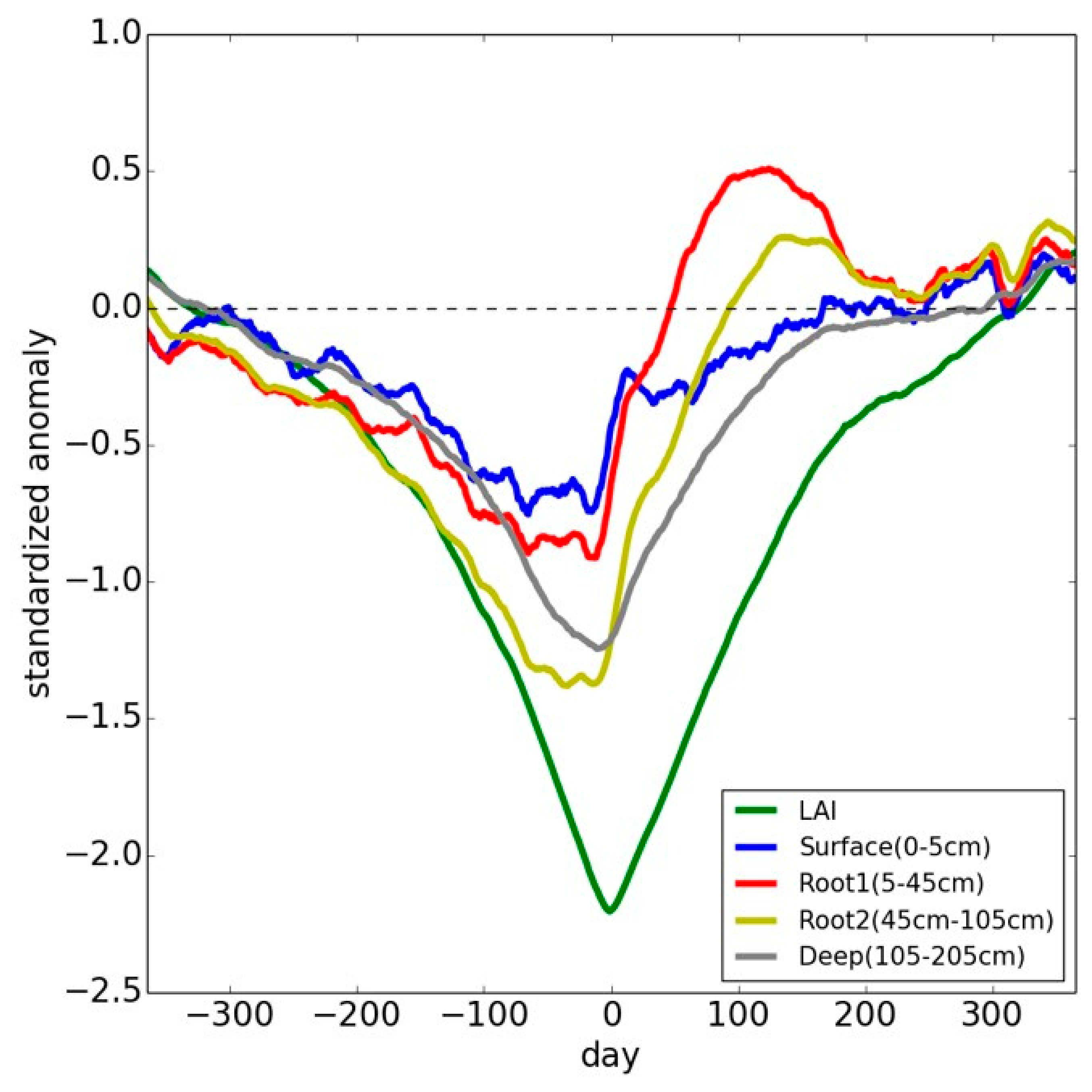
The spatiotemporally homogeneous land reanalysis dataset enables us to calculate a composite of the dynamics of soil moisture and vegetation in the extreme drought events. Figure 8 shows the composite of the LAI SA and the soil moisture SAs by averaging the SA time series of the 3499 identified drought events. Soil moisture in the shallow soil layers (i.e., surface, root 1, and root 2) has the quicker responses to rainfall deficits than soil moisture in the deep soil layer and LAI. Soil moisture in the depth of 0.05−1.05 m recovers from the drought condition quickly after day 0 and then becomes the wetter condition due to the reduction of transpiration caused by vegetation degradation.
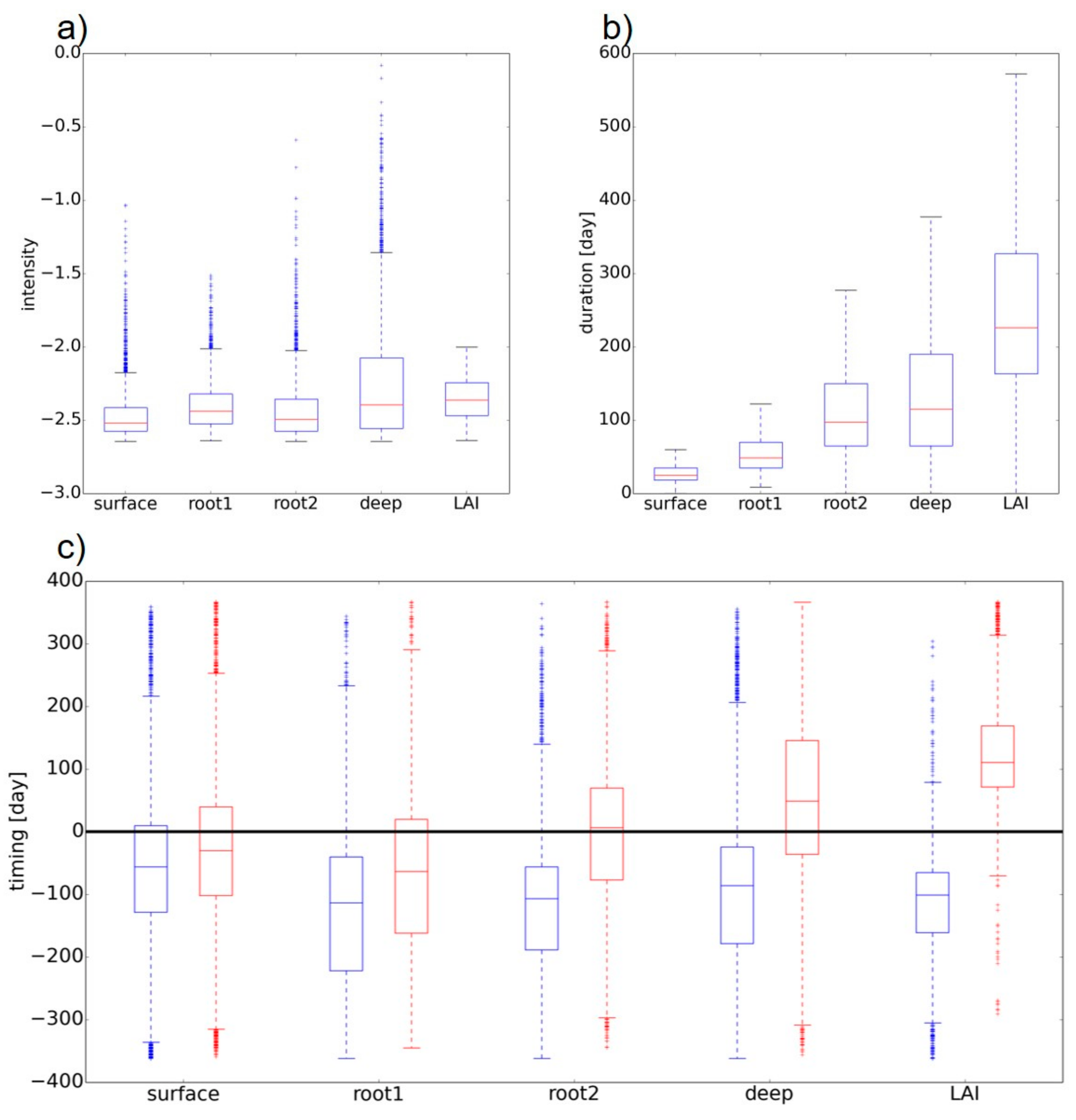
Figure 9 shows the boxplots of intensity, duration, and start and end date in the 3499 identified drought events (see Section 2.4). In most of the identified drought events with the LAI SA less than −2.0, the soil moisture SAs for all soil layers are also less than −2.0, which indicates that soil moisture in all soil layers is significantly degraded in the identified drought events (Figure 9a). The duration of the degradation of LAI and soil moisture in the deeper soil layers is longer than that of the soil moisture’s degradation in the shallower soil layers (Figure 9b). Figure 9c quantifies the drought propagation in the 3499 identified drought events. Soil moisture in the shallow layers (surface and root1) recovers from the drought condition before the climatological day-of-year of the LAI’s seasonal peak (i.e., day 0) in many drought events. On the other hand, soil moisture in the deeper soil layer (deep) recovers from the drought condition after the climatological day-of-year of the LAI’s seasonal peak on average. LAI has a much slower response to the rainfall deficit than soil moisture. In the median values of the days when the SAs have their minimum values, soil moisture in surface, root1, root2, and deep soil layers proceeds LAI by 63 days, 64 days, 47 days, and 19 days, respectively.
4. Discussions
4.1. Performance of ECHLA
I provided the new land reanalysis which explicitly simulates vegetation dynamics and evaluated its performance. It should be noted that there are three sources of errors, which need to be considered to interpret my verification study.
- Errors in meteorological forcings: The input of the LSM may be biased. The GLDAS meteorological forcings used in this study may have large biases especially in the poorly gauged regions.
- Errors in observations used for verification: The observations used for verification may be biased. The quality of the satellite products strongly depends on the skill of the algorithms to retrieve soil moisture and LAI from brightness temperature. Although in situ soil moisture observations may have relatively small instrument errors, they may not represent soil moisture in the coarse model grids.
- Errors in the data assimilation system: It includes the errors in the LSM, the RTM, and the data assimilation method.
Although I aim to quantify the third type of errors, it is generally difficult to decompose the bulk errors quantified by the metrics into the different types of errors.
Although there are high correlations between simulated LAI by ECHLA and satellite optically observed LAI, the absolute value of simulated LAI has the large deviation from that of satellite-observed LAI. Jarlan et al. [61] showed that simulated LAI by the ECMWF’s CTESSEL LSM deviates from MODIS LAI by a factor of 2. It is difficult to directly compare the absolute value of LSM-simulated LAI with that of satellite-observed LAI. It may be caused partly by the uncertainties in the satellite-observed LAI products [62].
There are two possible reasons why the data assimilation cannot improve the simulation of the absolute value of LAI. First, to solve the radiative transfer in the canopy, the information of vegetation water content and other parameters related to optical properties of plants is needed although the LSM directly solves carbon cycle. Therefore, I need to rely on some empirical equations to convert the LSM’s output to the RTM’s input (see Equations (8)–(11) in the Supplementary Materials), which induces uncertainties in the LDAS. Second, as Sawada et al. [55] indicated, the sensitivity of C- and X-band brightness temperature to vegetation becomes small when LAI becomes larger than 4 so that it is difficult to quantitatively constrain LAI in the forested area by assimilating the microwave signals.
It should be noted that the improvement of the representation of phenology by data assimilation positively impacts the identification and quantification of the drought propagation since I focused on the seasonal cycle of vegetation activity to identify the drought events (see Section 2.4). The increase of correlation coefficients between simulated and satellite-observed LAI improves the skill to estimate the timing of the beginning, end, and peak of seasons. It brings the accurate retrievals of the climatological day-of-year of the LAI’s seasonal peak, which positively impacts the identification and quantification of drought events based on the LAI’s time series.
The significant improvement of the surface soil moisture simulation by data assimilation can be found in the sparsely vegetated area when I compared the ECHLA simulation with both satellite and in situ observations. However, the impact of data assimilation on the simulation of sub-surface soil moisture was marginal in this study. The performance of ECHLA to simulate surface soil moisture is compatible to the other land reanalysis studies [14,36]. Assimilating satellite microwave brightness temperature observations reduces RMSEs against satellite surface soil moisture observations and in-situ surface soil moisture observations. The degradation of the skill to reproduce the satellite-observed surface soil moisture data can be found in the moderately and densely vegetated area. In the moderately and densely vegetated area, the uncertainty in the parameterization of the vegetation effect on microwave radiative transfer may degrade the skill to simulate the contribution of surface soil moisture to microwave brightness temperature. It should be noted that the accuracy of the satellite surface soil moisture observation product used for verification may also be low in the moderately and densely vegetated area [55,63]. Data assimilation has marginal impacts on correlation coefficients. This may be because the seasonal cycle of surface soil moisture is largely driven by the meteorological forcings and I did not consider the errors in the meteorological forcings in the data assimilation system. It may be beneficial to use multiple meteorological forcing datasets to consider their errors.
Few previous studies have evaluated the skill of LDASs to simulate sub-surface soil moisture. Sawada et al. [40] have found that CLVDAS can improve sub-surface soil moisture by solving the inversion problem to estimate root-zone soil moisture from vegetation growth on land surface. While Sawada et al. [40] evaluated the performance of CLVDAS in a single meteorological observation site using accurate in situ meteorological forcings’ observation, I found an improvement of the sub-surface soil moisture simulation in two of the four in situ observation sites in the semi-global application of this study. The improvement of the sub-surface soil moisture simulation contributes to the drought analysis since sub-surface soil moisture has an important role in the drought propagation. It should be noted that the errors in in situ sub-surface soil moisture observations may be larger than those in in situ surface soil moisture observations. When installing observation probes in deep soil, soil structure may be somewhat disturbed so that it is unclear if the in situ observation represents sub-surface soil moisture in the coarse model grid. In addition, there are uncertainties in the depths of soil moisture measurements. The degradation of correlation coefficients in the AMMA-CATCH Tondikiboro site by data assimilation may be caused partly by these representation errors in the in-situ observations.
To improve the skill of ECHLA to simulate soil moisture and LAI, the parameter optimization of the LSM should be implemented although I optimized only the parameter of the RTM in this paper. Sawada and Koike [39] optimized the unknown hydrological and ecological parameters of the LSM (e.g., hydraulic conductivity), by assimilating microwave brightness temperature observations and improved the skill of the LSM to simulate both surface soil moisture and LAI. Optimizing unknown parameters of LSMs by data assimilation has been intensively investigated [28,29,30]. Although the parameter optimization module is included in the current version of CLVDAS used in this study, I did not apply it to optimize the unknown parameters of the LSM in the semi-global application of this study because it is computationally demanding. I should explore the computationally efficient parameter optimization method, which can be applied globally, in the future
4.2. Conceptual Model of the Ecohydrological Drought Propagation
On average, the drought events identified in this study significantly damage both vegetation activity and soil water storage from the surface to deep soil layers. The degradation of vegetation dynamics lasts 150–350 days while the duration of soil moisture deficits is shorter than that of vegetation degradation. The identified drought events start approximately 100 days before the climatological day-of-year of the LAI’s seasonal peak. Soil moisture in the shallow soil layers quickly recovers from the drought condition before the climatological day-of-year of the LAI’s seasonal peak while soil moisture in the deep soil layers and vegetation dynamics recover from the drought condition approximately 100 days after the climatological day-of-year of the LAI’s seasonal peak.
This drought propagation from soil moisture to vegetation has been found by previous studies. Sepulcre-Canto et al. [10] found that a soil moisture index calculated by a precipitation-runoff model is significantly correlated with the anomaly of the satellite-observed fraction of absorbed photosynthetically active radiation (fAPAR) when soil moisture proceeds fAPAR by 10–20 days in Europe. Akarsh and Mishra [11] showed that the root-zone (top 60 cm) soil moisture anomaly calculated by GLDAS is strongly correlated with the anomaly of satellite-observed normalized difference vegetation index (NDVI) when soil moisture proceeds NDVI by 1 month in India. I support these regional findings using a composite of soil moisture and LAI in the global snow-free region, which are simulated by the new land reanalysis.
It should be noted that the farmer’s strategy of planting and harvesting was not considered in the LSM. Ignoring the farmer’s adaptation strategy against severe drought events may overestimate the negative impact of water deficits in this study. In addition, I focused only on the effect of water deficits on agricultural activities and many other factors which harm agricultural activities were not considered. For instance, crops are greatly affected by floods and associated inundation. Any political and economic effects on agriculture are not considered in the drought identification and quantification method used in this study.
The major limitation of this study is that the study period is short to identify the extreme drought events. To obtain an inclusive drought catalog using ECHLA, I need to extend the study period which is currently identical to the AMSR-E operational period. Since I directly assimilate satellite-observed brightness temperature observations instead of derived products, it is straightforward to assimilate observations from the other satellites such as AMSR2, Soil Moisture, Ocean Salinity (SMOS), and Soil Moisture Active Passive (SMAP). However, it should be noted that changes in observing systems used for data assimilation may cause temporal inhomogeneity in the reanalysis dataset [64,65]. The period of ECHLA will be extended to obtain an inclusive drought catalog.
5. Conclusions
I provided a semi-global land reanalysis which explicitly calculates vegetation growth and senescence and is constrained by satellite microwave observations. I revealed that the new land reanalysis had the reasonable skill to simulate surface soil moisture, sub-surface soil moisture, and LAI and was useful to identify and quantify the drought propagation. By analyzing the SAs of soil moisture and LAI in the land reanalysis, I identified the severe drought events and quantified the drought propagation from surface soil moisture to sub-surface soil moisture and the corresponding vegetation dynamics. On average, the drought events identified in this study significantly damage both vegetation activity and soil water storage from the surface to deep soil layers. Soil moisture in the shallow soil layers quickly recovers from the drought condition while the deficits of soil moisture in the deep soil layers and vegetation dynamics lasted until approximately 100 days after the climatological day-of-year of the LAI’s seasonal peak.
Supplementary Materials
The following are available online at https://www.mdpi.com/2072-4292/10/8/1197/s1, Text S1: Formulations of Coupled Land and Vegetation Data Assimilation System (CLVDAS).
Funding
This research was funded by the JSPS KAKENHI Grant Number JP17K18352, Data Integration and Analysis System (DIAS), JAXA, and the FLAGSHIP2020 project of the Ministry of Education, Culture, Sports, Science, and Technology.
Acknowledgments
The GLDAS data products were provided by the National Aeronautics and Space Administration (NASA) and can be downloaded at http://disc.sci.gsfc.nasa.gov/hydrology/data-holdings. The AMSR-E brightness temperature observation data products were provided by the Japan Aerospace Exploration Agency (JAXA) and can be downloaded at https://gcom-w1.jaxa.jp/auth.html. The GLASS LAI data products were provided by Global Land Cover Facility (GLCF) and can be downloaded at http://www.glcf.umd.edu/data/lai/. The ESA CCI surface soil moisture product was provided by ESA and can be downloaded at http://www.esa-soilmoisture-cci.org/. The in situ soil moisture observations were archived at International Soil Moisture Network (ISMN) https://ismn.geo.tuwien.ac.at/. The numerical experiments were implemented using the Oakleaf-FX supercomputer furnished by Supercomputing Division, Information Technology Center, the University of Tokyo. I thank three anonymous reviewers for their helpful comments.
Conflicts of Interest
The author declares no conflicts of interest.
References
- Wilhite, D.A. Drought: A Global Assessment; Routledge: London, UK, 2000. [Google Scholar]
- Svoboda, M.; LeComte, D.; Hayes, M.; Heim, R.; Gleason, K.; Angel, J.; Rippey, B.; Tinker, R.; Palecki, M.; Stooksbury, D.; et al. The drought monitor. Bull. Am. Meteorol. Soc. 2002, 83, 1181–1190. [Google Scholar] [CrossRef]
- Anderson, W.; Zaitchik, B.F.; Hain, C.R.; Anderson, M.C.; Yilmaz, M.T.; Mecikalski, J.; Schultz, L. Towards an integrated soil moisture drought monitor for East Africa. Hydrol. Earth Syst. Sci. 2012, 16, 2893–2913. [Google Scholar] [CrossRef] [Green Version]
- McNally, A.; Arsenault, K.; Kumar, S.; Shukla, S.; Peterson, P.; Wang, S.; Funk, C.; Peters-Lidard, C.D.; Verdin, J.P. A land data assimilation system for sub-Saharan Africa food and water security applications. Sci. Data 2017, 4. [Google Scholar] [CrossRef] [PubMed]
- Yuan, X.; Wood, E.F. Multimodel seasonal forecasting of global drought onset. Geophys. Res. Lett. 2013, 40, 4900–4905. [Google Scholar] [CrossRef] [Green Version]
- Pan, M.; Yuan, X.; Wood, E.F. A probabilistic framework for assessing drought recovery. Geophys. Res. Lett. 2013, 14, 3637–3642. [Google Scholar] [CrossRef]
- Sawada, Y.; Koike, T. Towards ecohydrological drought monitoring and prediction using a land data assimilation system: A case study on the Horn of Africa drought (2010–2011). J. Geophys. Res. Atmos. 2016, 121, 8229–8242. [Google Scholar] [CrossRef]
- Wilhite, D.A.; Glantz, M.H. Understanding: The Drought Phenomenon: The Role of Definitions. Water Int. 1985, 10. [Google Scholar] [CrossRef]
- Sawada, Y.; Koike, T.; Jaranilla-Sanchez, P.A. Modeling hydrologic and ecologic responses using a new eco-hydrological model for identification of droughts. Water Resour. Res. 2014, 50. [Google Scholar] [CrossRef]
- Sepulcre-Canto, G.; Horion, S.; Singleton, A.; Carrao, H.; Vogt, J. Development of a Combined Drought Indicator to detect agricultural drought in Europe. Nat. Harzards Earth Syst. Sci. 2012, 12, 3519–3531. [Google Scholar] [CrossRef] [Green Version]
- Akarsh, A.; Mishra, V. Prediction of vegetation anomalies to improve food security and water management in India. Geophys. Res. Lett. 2015, 42, 5290–5298. [Google Scholar] [CrossRef] [Green Version]
- Rodell, M.; Houser, P.R.; Jambor, U.; Gottschalck, J.; Mitchell, K.; Meng, C.-J.; Arsenault, K.; Cosgrove, B.; Radakovich, J.; Bosilovich, M.; et al. The global land data assimilation system. Bull. Am. Meteorol. Soc. 2004, 85, 381–394. [Google Scholar] [CrossRef]
- Reichle, R.H.; Koster, R.D.; De Lannoy, G.J.M.; Forman, B.M.; Liu, Q.; Mahanama, S.P.P.; Touré, A. Assessment and Enhancement of MERRA Land Surface Hydrology Estimates. J. Clim. 2011, 24, 6322–6338. [Google Scholar] [CrossRef] [Green Version]
- Balsamo, G.; Albergel, C.; Beljaars, A.; Boussetta, S.; Brun, E.; Cloke, H.; Dee, D.; Dutra, E.; Muñoz-Sabater, J.; Pappenberger, F.; et al. ERA-Interim/Land: A global land surface reanalysis data set. Hydrol. Earth Syst. Sci. 2015, 19, 389–407. [Google Scholar] [CrossRef]
- Tang, J.; Cheng, H.; Liu, L. Assessing the recent droughts in Southwestern China using satellite gravimetry. Water Resour. Res. 2014, 50, 3030–3038. [Google Scholar] [CrossRef] [Green Version]
- Leblanc, M.; Tregoning, J.P.; Ramillien, G.; Tweed, S.O.; Fakes, A. Basin-scale, integrated observations of the early 21st century multiyear drought in Southeast Australia. Water Resour. Res. 2009, 45, W04408. [Google Scholar] [CrossRef]
- Asoka, A.; Glesson, T.; Wada, Y.; Mishra, V. Relative contribution of monsoon precipitation and pumping to changes in groundwater storage in India. Nat. Geosci. 2017, 10, 109–117. [Google Scholar] [CrossRef] [Green Version]
- Yuan, X.; Ma, Z.; Pan, M.; Shi, C. Microwave remote sensing of short-term droughts during crop growing seasons. Geophys. Res. Lett. 2015, 42, 4394–4401. [Google Scholar] [CrossRef] [Green Version]
- Hao, Z.; Aghakouchak, A. A Nonparametric Multivariate Multi-Index Drought Monitoring Framework. J. Hydrometeorol. 2014, 15, 89–101. [Google Scholar] [CrossRef]
- Madadgar, S.; AghaKouchak, A.; Farahmand, A.; Davis, S.J. Probabilistic estimates of drought impacts on agricultural production. Geophys. Res. Lett. 2017, 44. [Google Scholar] [CrossRef]
- Ulaby, F.; Moore, R.K.; Fung, A. (Eds.) Microwave Remote Sensing: Active and Passive—Volume Scattering and Emission Theory; Artech House: Dedham, MA, USA, 1986; Volume 3. [Google Scholar]
- Paloscia, S.; Pampaloni, P. Microwave polarization index for monitoring vegetation growth. IEEE Trans. Geosci. Remote 1988, 26, 617–621. [Google Scholar] [CrossRef]
- Owe, M.; de Jeu, R.; Walker, J. A methodology for surface soil moisture and vegetation optical depth retrieval using the microwave polarization difference index. IEEE Trans. Geosci. Remote 2001, 39, 1643–1654. [Google Scholar] [CrossRef] [Green Version]
- Fujii, H.; Koike, T.; Imaoka, K. Improvement of the AMSR-E Algorithm for Soil Moisture Estimation by Introducing a Fractional Vegetation Coverage Dataset Derived from MODIS Data. J. Remote Sens. Soc. Jpn. 2009, 29, 282–292. [Google Scholar]
- Holmes, T.R.H.; De Jeu, R.A.M.; Owe, M.; Dolman, A.J. Land surface temperature from Ka band (37 GHz) passive microwave observations. J. Geophys. Res. 2009, 114, D04113. [Google Scholar] [CrossRef]
- Kerr, Y.H.; Font, J.; Martin-Neira, M.; Mecklenburg, S. Introduction to the Special Issue on the ESA’s Soil Moisture and Ocean Salinity Mission (SMOS)—Instrument performance and first results. IEEE Trans. Geosci. Remote Sens. 2012, 50, 1351–1353. [Google Scholar] [CrossRef] [Green Version]
- Chan, S.K.; Bindlish, R.; O’Neill, P.; Jackson, T.; Njoku, E.; Dunbar, S.; Chaubell, J.; Piepmeier, J.; Yueh, S.; Entekhabi, D.; et al. Development and assessment of the SMAP enhanced passive soil moisture product. Remote Sens. Environ. 2016, 204, 931–941. [Google Scholar] [CrossRef]
- Yang, K.; Watanabe, T.; Koike, T.; Li, X.; Fujii, H.; Tamagawa, K.; Ma, Y.; Ishikawa, H. Auto-calibration System Developed to Assimilate AMSR-E Data into a Land Surface Model for Estimating Soil Moisture and the Surface Energy Budget. J. Meteorol. Soc. Jpn. 2007, 85A, 229–242. [Google Scholar] [CrossRef]
- Tian, X.; Xie, Z.; Dai, A.; Shi, C.; Jia, B.; Chen, F.; Yang, K. A dual-pass variational data assimilation framework for estimating soil moisture profiles from AMSR-E microwave brightness temperature. J. Geophys. Res. 2009, 114, D16102. [Google Scholar] [CrossRef]
- Yang, K.; Koike, T.; Kaihotsu, I.; Qin, J. Validation of a Dual-Pass Microwave Land Data Assimilation System for Estimating Surface Soil Moisture in Semiarid Regions. J. Hydrometeorol. 2009, 10, 780–793. [Google Scholar] [CrossRef]
- Qin, J.; Liang, S.; Yang, K.; Kaihotsu, I.; Liu, R.; Koike, T. Simultaneous estimation of both soil moisture and model parameters using particle filtering method through the assimilation of microwave signal. J. Geophys. Res. 2009, 114, D15103. [Google Scholar] [CrossRef]
- Kumar, S.; Reichle, V.R.H.; Koster, R.D.; Crow, W.T.; Peters-Lidard, C.D. Role of Subsurface Physics in the Assimilation of Surface Soil Moisture Observations. J. Hydrometeorol. 2009, 10, 1534–1547. [Google Scholar] [CrossRef] [Green Version]
- Li, B.; Toll, D.; Zhan, X.; Cosgrove, B. Improving estimated soil moisture fields through assimilation of AMSR-E soil moisture retrievals with an ensemble Kalman filter and a mass conservation constraint. Hydrol. Earth Syst. Sci. 2012, 16, 105–119. [Google Scholar] [CrossRef] [Green Version]
- Su, Z.; de Rosnay, P.; Wen, J.; Wang, L.; Zeng, Y. Evaluation of ECMWF’s soil moisture analyses using observations on the Tibetan Plateau. J. Geophys. Res. Atmos. 2013, 118, 5304–5318. [Google Scholar] [CrossRef]
- He, L.; Chen, J.M.; Liu, J.; Belair, S.; Luo, X. Assessment of SMAP soil moisture for global simulation of gross primary production. J. Geophys. Res. Biogeosci. 2017, 122, 1549–1563. [Google Scholar] [CrossRef]
- Kumar, S.V.; Peters-Lidard, C.D.; Mocko, D.; Reichle, R.H.; Liu, Y.; Arsenault, K.R.; Xia, Y.; Ek, M.; Riggs, G.; Livneh, B.; et al. Assimilation of Remotely Sensed Soil Moisture and Snow Depth Retrievals for Drought Estimation. J. Hydrometeorol. 2014, 15, 2446–2469. [Google Scholar] [CrossRef]
- Bardu, A.L.; Calvet, J.-C.; Mahfouf, J.-F.; Albergel, C.; Lafont, S. Assimilation of Soil Wetness Index and Leaf Area Index into the ISBA-A-gs land surface model: Grassland case study. Biogeosciences 2011, 8, 1971–1986. [Google Scholar] [CrossRef] [Green Version]
- Liu, P.-W.; Bongiovanni, T.; Monsivais-Huertero, A.; Judge, J.; Steele-Dunne, S.; Bindlish, R.; Jackson, T.J. Assimilation of Active and Passive Microwave Observations for Improved Estimates of Soil Moisture and Crop Growth. IEEE J. Sel. Top. Appl. Earth Observ. Remote Sens. 2016, 9, 1357–1369. [Google Scholar] [CrossRef]
- Sawada, Y.; Koike, T. Simultaneous estimation of both hydrological and ecological parameters in an ecohydrological model by assimilating microwave signal. J. Geophys. Res. Atmos. 2014, 119. [Google Scholar] [CrossRef]
- Sawada, Y.; Koike, T.; Walker, J.P. A land data assimilation system for simultaneous simulation of soil moisture and vegetation dynamics. J. Geophys. Res. Atmos. 2015, 120. [Google Scholar] [CrossRef]
- Sheffield, J.; Goteti, G.; Wood, E.F. Development of a 50-Year High-Resolution Global Dataset of Meteorological Forcings for Land Surface Modeling. J. Clim. 2006, 19, 3088–3111. [Google Scholar] [CrossRef]
- Kachi, M.; Naoki, K.; Hori, M.; Imaoka, K. AMSR2 validation results. In Proceedings of the 2013 IEEE International Geoscience and Remote Sensing Symposium (IGARSS), Melbourne, VIC, Australia, 21–26 July 2013; pp. 831–834. [Google Scholar] [CrossRef]
- Liu, Y.Y.; de Jeu, R.A.M.; McCabe, M.F.; Evans, J.P.; van Dijk, A.I.J.M. Global long-term passive microwave satellite-based retrievals of vegetation optical depth. Geophys. Res. Lett. 2011, 38, L18402. [Google Scholar] [CrossRef]
- Global Soil Data Task Group, Global Gridded Surfaces of Selected Soil Characteristics (IGBPDIS). 2000. Available online: https://daac.ornl.gov (accessed on 13 February 2018).
- Food and Agricultural Organization, Digital Soil Map of the World and Derived Soil Properties, Land Water Digital Media Ser. 1 [CR-ROM], Rome. 2003. Available online: http://www.fao.org/ag/agl/lwdms.stm (accessed on 13 February 2018).
- Xiao, Z.; Liang, S.; Wang, J.; Chen, P.; Yin, X.; Zhang, L.; Song, J. Use of General Regression Neural Networks for Generating the GLASS Leaf Area Index Product from Time Series MODIS Surface Reflectance. IEEE Trans. Geosci. Remote Sens. 2013, 52, 209–223. [Google Scholar] [CrossRef]
- Huang, D.; Knyazikhin, Y.; Wang, W.; Deering, D.W.; Stenberg, P.; Shabanov, N.V.; Tan, B.; Myneni, R.B. Stochastic transport theory for investigating the three-dimensional canopy structure from space measurements. Remote Sens. Environ. 2008, 112, 35–50. [Google Scholar] [CrossRef]
- Dorigo, W.A.; Wagner, W.; Albergel, C.; Albrecht, F.; Balsamo, G.; Brocca, L.; Chung, D.; Ertl, M.; Forkel, M.; Gruber, A.; et al. ESA CCI Soil Moisture for improved Earth system understanding: State-of-the art and future directions. Remote Sens. Environ. 2017, 15, 185–215. [Google Scholar] [CrossRef]
- Gruber, A.; Dorigo, W.A.; Crow, W.; Wagner, W. Triple Collocation-Based Merging of Satellite Soil Moisture Retrievals. IEEE Trans. Geosci. Remote 2017, 55, 6780–6792. [Google Scholar] [CrossRef]
- Liu, Y.Y.; Dorigo, W.A.; Parinussa, R.M.; de Jeu, R.; Wagner, W.; McCabe, M.F.; Evans, J.P.; van Dijk, A.I.J.M. Trend-preserving blending of passive and active microwave soil moisture retrievals. Remote Sens. Environ. 2012, 123, 280–297. [Google Scholar] [CrossRef]
- Dorigo, W.A.; Wagner, W.; Hohensinn, R.; Hahn, S.; Paulik, C.; Drusch, M.; Mecklenburg, S.; van Oevelen, P.; Robock, A.; Jackson, T. The International Soil Moisture Network: A data hosting facility for global in situ soil moisture measurements. Hydrol. Earth Syst. Sci. 2011, 15, 1675–1698. [Google Scholar] [CrossRef]
- Lebel, T.; Cappelaere, B.; Galle, S.; Hanan, N.; Kergoat, L.; Levis, S.; Vieux, B.; Descroix, L.; Gosset, M.; Mougin, E.; et al. AMMA-CATCH studies in the Sahelian region of West-Africa: An overview. J. Hydrol. 2009, 375, 3–13. [Google Scholar] [CrossRef] [Green Version]
- Ardö, J. A 10-Year Dataset of Basic Meteorology and Soil Properties in Central Sudan. Dataset Pap. Geosci. 2013, 2013, 297973. [Google Scholar] [CrossRef]
- Tagesson, T.; Fensholt, R.; Guiro, I.; Rasmussen, M.O.; Huber, S.; Mbow, C.; Garcia, M.; Horion, S.; Sandholt, I.; Holm-Rasmussen, B.; et al. Ecosystem properties of semiarid savanna grassland in West Africa and its relationship with environmental variability. Glob. Chang. Biol. 2015, 21, 250–264. [Google Scholar] [CrossRef] [PubMed]
- Sawada, Y.; Tsutsui, H.; Koike, T. Ground Truth of Passive Microwave Radiative Transfer on Vegetated Land Surfaces. Remote Sens. 2017, 9, 655. [Google Scholar] [CrossRef]
- Duan, Q.; Sorooshian, S.; Gupta, V. Effective and Efficient Global Optimization for Conceptual Rainfall-Runoff Models. Water Resour. Res. 1992, 28, 1015–1031. [Google Scholar] [CrossRef]
- Jackson, R.B.; Canadell, J.G.; Ehleringer, J.R.; Mooney, H.A.; Sala, O.E.; Schulze, E.D. A global analysis of root distributions for terrestrial biomes. Oecologia 1996, 108, 389–411. [Google Scholar] [CrossRef] [PubMed]
- Minamide, M.; Zhang, F. Adaptive Observation Error Inflation for Assimilating All-Sky Satellite Radiance. Mon. Weather Rev. 2017, 145, 1063–1081. [Google Scholar] [CrossRef]
- Jaranilla-Sanchez, P.A.; Wang, L.; Koike, T. Modeling the hydrological responses of the Pampanga River basin, Philippines: A quantitative approach for identifying droughts. Water Resour. Res. 2011, 47, W03514. [Google Scholar] [CrossRef]
- Jonsson, P.; Eklundh, L. TIMESAT—A program for analysing time-series of satellite sensor data. Comput. Geosci. 2004, 30, 833–845. [Google Scholar] [CrossRef]
- Jarlan, L.; Balsamo, G.; Lafont, S.; Beljaars, A.; Calvet, J.-C.; Mougin, E. Analysis of leaf area index in the ECMWF land surface model and impact on latent heat and carbon fluxes: Application to West Africa. J. Geophys. Res. 2008, 113, D24117. [Google Scholar] [CrossRef]
- Liu, Y.; Xiao, J.; Ju, W.; Zhu, G.; Wu, X.; Fan, W.; Li, D.; Zhou, Y. Satellite-derived LAI products exhibit large discrepancies and can lead to substantial uncertainty in simulated carbon and water fluxes. Remote Sens. Environ. 2018, 206, 174–188. [Google Scholar] [CrossRef]
- Crow, W.T.; Chan, S.; Entekhabi, D.; Hsu, A.; Jackson, T.J.; Njoku, E.; O’Neill, P.; Shi, J. An observing system simulation experiment for hydros radiometer-only soil moisture and freeze-thaw products. IEEE Trans. Geosci. Remote 2005, 43, 1289–1303. [Google Scholar] [CrossRef]
- Kobayashi, C.; Endo, H.; Ota, Y.; Kobayashi, S.; Onoda, H.; Harada, Y.; Onogi, K.; Kamahori, H. Preliminary Results of the JRA-55C, an Atmospheric Reanalysis Assimilating Conventional Observations Only. SOLA 2014, 10, 78–82. [Google Scholar] [CrossRef] [Green Version]
- Kobayashi, S.; Ota, Y.; Harada, Y.; Ebita, A.; Moriya, M.; Onoda, H.; Onogi, K.; Kamahori, H.; Kobayashi, C.; Endo, H.; et al. The JRA-55 Reanalysis: General Specifications and Basic Characteristics. J. Meteorol. Soc. Jpn. 2015, 93, 5–48. [Google Scholar] [CrossRef] [Green Version]
Figure 1.
Study area (red) and the locations of the in situ observation sites of the DAHRA (purple rectangle), CARBOAFRICA (blue circle), AMMA-CATCH Belefoungou in Benin (black rectangle), and AMMA-CATCH Tondikiboro in Niger (yellow circle) networks.
Figure 1.
Study area (red) and the locations of the in situ observation sites of the DAHRA (purple rectangle), CARBOAFRICA (blue circle), AMMA-CATCH Belefoungou in Benin (black rectangle), and AMMA-CATCH Tondikiboro in Niger (yellow circle) networks.

Figure 2.
Schematic of production steps of ECHLA. See Section 2.2 and Section 2.3, and the Supplementary Materials for details.
Figure 2.
Schematic of production steps of ECHLA. See Section 2.2 and Section 2.3, and the Supplementary Materials for details.

Figure 3.
(a) The climatological day-of-year (DOY) of the ECoHydrological Land reAnalysis (ECHLA)-simulated leaf area index’s (LAI’s) seasonal peak averaged from 2003 to 2010. (b) Schematic of the drought detection method. Black dashed line shows the timing of the climatological LAI’s seasonal peak. See Section 2.4 for details.

Figure 4.
Performance of ECHLA to reproduce satellite-observed LAI (GLASS LAI). (a) Correlation coefficient and (b) RMSE [m2/m2] of simulated LAI by the DA experiment. The differences of (c) correlation coefficient and (d) RMSE between the DA experiment and the OL experiment.
Figure 4.
Performance of ECHLA to reproduce satellite-observed LAI (GLASS LAI). (a) Correlation coefficient and (b) RMSE [m2/m2] of simulated LAI by the DA experiment. The differences of (c) correlation coefficient and (d) RMSE between the DA experiment and the OL experiment.

Figure 5.
Performance of ECHLA to reproduce satellite-observed surface soil moisture (ESA CCI SM). (a) Correlation coefficient and (b) RMSE [m3/m3] of simulated surface soil moisture by the DA experiment. The differences of (c) correlation coefficient and (d) RMSE between the DA experiment and the OL experiment. ESA CCI SM does not provide surface soil moisture retrievals in the dense vegetated area and the performance of ECHLA was not evaluated there.

Figure 6.
The locations of the identified drought events. Each dot shows the location of the identified drought event. The color of dots shows the year when the identified drought event occurred. The identified droughts shown by black, red, green, blue, yellow, and purple occurred in 2004, 2005, 2006, 2007, 2008, and 2009, respectively.

Figure 7.
Time series of SAs of soil moisture in surface (0–0.05 m) (blue), root1 (0.05–0.45 m) (red), root2 (0.45–1.05 m) (yellow), and deep (1.05–2.05 m) (grey) soil layers, and LAI (green) for the identified drought events of (a) Ethiopia in 2005 (36.375E; 10.25N), (b) India in 2009 (81.125E; 22.75N), (c) Thailand in 2005 (99.875E; 14.25N), and (d) Brazil in 2007 (46.125W; 9S). The climatological day-of-year of the LAI’s seasonal peak is set to day 0.

Figure 8.
Composite of the identified drought events’ SAs of LAI (green), surface (0–0.05 m) (blue), root1 (0.05–0.45 m) (red), root2 (0.45–1.05 m) (yellow), and deep (1.05–2.05 m) (grey) soil layers in the global snow-free region. The climatological day-of-year of the LAI’s seasonal peak is set to day 0.

Figure 9.
(a) Boxplot of intensity of SAs in the 3499 identified drought events. (b) Same as (a) but for duration. (c) Same as (a) but for the start date (blue) and the end date (red). Outliers are larger (smaller) than Q3 + interquartile range (Q1—interquartile range). See Section 2.4 for the definitions of intensity, duration, and the start and end date of droughts used in this study.


Table 1.
RMSE, ubRMSE, and correlation coefficient of soil moisture simulated by the DA experiment and the OL experiment compared to the in situ observation data in the DAHRA site.
Table 1.
RMSE, ubRMSE, and correlation coefficient of soil moisture simulated by the DA experiment and the OL experiment compared to the in situ observation data in the DAHRA site.
| Depth [m] | RMSE [m3/m3] | ubRMSE [m3/m3] | R | |
|---|---|---|---|---|
| 0.05 | DA | 0.079 | 0.057 | 0.42 |
| OL | 0.091 | 0.075 | 0.45 | |
| 0.10 | DA | 0.13 | 0.022 | 0.61 |
| OL | 0.16 | 0.023 | 0.42 | |
| 0.30 | DA | 0.13 | 0.021 | 0.61 |
| OL | 0.16 | 0.019 | 0.53 | |
| 0.50 | DA | 0.13 | 0.019 | 0.66 |
| OL | 0.16 | 0.018 | 0.54 | |
| 1.00 | DA | 0.13 | 0.021 | 0.54 |
| OL | 0.16 | 0.023 | 0.46 |
Table 2.
Same as Table 1 but for the in situ observation data in the CARBO AFRICA site.
Table 2.
Same as Table 1 but for the in situ observation data in the CARBO AFRICA site.
| Depth [m] | RMSE [m3/m3] | ubRMSE [m3/m3] | R | |
|---|---|---|---|---|
| 0.05 | DA | 0.086 | 0.035 | 0.67 |
| OL | 0.092 | 0.039 | 0.72 | |
| 0.15 | DA | 0.12 | 0.026 | 0.68 |
| OL | 0.15 | 0.022 | 0.56 | |
| 0.30 | DA | 0.092 | 0.023 | 0.66 |
| OL | 0.12 | 0.017 | 0.65 | |
| 0.60 | DA | 0.082 | 0.022 | 0.56 |
| OL | 0.12 | 0.018 | 0.56 | |
| 1.00 | DA | 0.12 | 0.020 | 0.41 |
| OL | 0.16 | 0.020 | 0.45 | |
| 1.50 | DA | 0.12 | 0.024 | 0.20 |
| OL | 0.17 | 0.021 | 0.39 | |
| 2.00 | DA | 0.12 | 0.027 | −0.03 |
| OL | 0.17 | 0.024 | 0.30 |
Table 3.
Same as Table 1 but for the in situ observation data in the AMMA-CATCH Belefoungou site.
Table 3.
Same as Table 1 but for the in situ observation data in the AMMA-CATCH Belefoungou site.
| Depth [m] | RMSE [m3/m3] | ubRMSE [m3/m3] | R | |
|---|---|---|---|---|
| 0.05 | DA | 0.064 | 0.051 | 0.86 |
| OL | 0.068 | 0.064 | 0.86 | |
| 0.10 | DA | 0.082 | 0.049 | 0.86 |
| OL | 0.086 | 0.051 | 0.85 | |
| 0.20 | DA | 0.072 | 0.049 | 0.84 |
| OL | 0.075 | 0.049 | 0.86 | |
| 0.40 | DA | 0.063 | 0.051 | 0.83 |
| OL | 0.059 | 0.049 | 0.88 | |
| 0.60 | DA | 0.053 | 0.046 | 0.85 |
| OL | 0.050 | 0.044 | 0.89 | |
| 1.00 | DA | 0.058 | 0.031 | 0.81 |
| OL | 0.049 | 0.024 | 0.91 |
Table 4.
Same as Table 1 but for the in situ observation data in the AMMA-CATCH Tondikiboro site.
Table 4.
Same as Table 1 but for the in situ observation data in the AMMA-CATCH Tondikiboro site.
| Depth [m] | RMSE [m3/m3] | ubRMSE [m3/m3] | R | |
|---|---|---|---|---|
| 0.05 | DA | 0.078 | 0.044 | 0.65 |
| OL | 0.067 | 0.062 | 0.75 | |
| 0.10 | DA | 0.15 | 0.025 | 0.54 |
| OL | 0.15 | 0.020 | 0.66 | |
| 0.4–0.7 | DA | 0.16 | 0.021 | 0.53 |
| OL | 0.16 | 0.016 | 0.68 | |
| 0.7–1.0 | DA | 0.16 | 0.021 | 0.44 |
| OL | 0.17 | 0.016 | 0.61 | |
| 1.05–1.35 | DA | 0.19 | 0.018 | 0.34 |
| OL | 0.19 | 0.014 | 0.55 |
© 2018 by the author. Licensee MDPI, Basel, Switzerland. This article is an open access article distributed under the terms and conditions of the Creative Commons Attribution (CC BY) license (http://creativecommons.org/licenses/by/4.0/).
Share and Cite
MDPI and ACS Style
Sawada, Y. Quantifying Drought Propagation from Soil Moisture to Vegetation Dynamics Using a Newly Developed Ecohydrological Land Reanalysis. Remote Sens. 2018, 10, 1197. https://doi.org/10.3390/rs10081197
AMA Style
Sawada Y. Quantifying Drought Propagation from Soil Moisture to Vegetation Dynamics Using a Newly Developed Ecohydrological Land Reanalysis. Remote Sensing. 2018; 10(8):1197. https://doi.org/10.3390/rs10081197
Chicago/Turabian StyleSawada, Yohei. 2018. "Quantifying Drought Propagation from Soil Moisture to Vegetation Dynamics Using a Newly Developed Ecohydrological Land Reanalysis" Remote Sensing 10, no. 8: 1197. https://doi.org/10.3390/rs10081197
Note that from the first issue of 2016, this journal uses article numbers instead of page numbers. See further details here.