Experimental Study of Flow-Induced Whistling in Pipe Systems Including a Corrugated Section

Abstract

When air flows through pipe systems that include a corrugated segment, a whistling tone is generated and increases in intensity with increasing flow velocity. This whistling sound is related to the particular geometry of corrugated pipes, which is in the form of alternating cavities. This whistling is an environmental noise problem as well as a possible structural danger because of the resulting induced vibration. This paper studies the whistling behavior of various pipe systems with a combination of smooth and corrugated pipes through a series of experiments. The considered pipe systems consist of two smooth pipes attached at the upstream and downstream ends of a corrugated segment. Experiments with smooth and corrugated pipes, which had inner diameters of 15.25 and 16.5 mm, respectively, and various lengths, were performed for flow velocities of up to approximately 30 m/s. The minimum and maximum Strouhal numbers ($St$) obtained during our experiments were 0.25 and 0.38, respectively. For all pipe configurations investigated in this study, the lowest Mach number at which whistling was observed was 0.017, and the maximum was 0.093. The lowest frequency at which whistling was detected in our experiments was 650 Hz, and the highest was 3080 Hz. The results presented in the form of different variables and dimensionless parameters, including the frequency, Mach number, Strouhal number, and Helmholtz number. The average mode gap and number of excited acoustic modes were also taken into account for all considered configurations. The pipe systems with longer corrugated segments had broader whistling ranges than did configurations with shorter segments, indicating that the number of cavities inside the corrugated pipe has a direct effect on whistling. Increasing the smooth pipe length (either upstream or downstream) resulted in a decrease in the average mode gap between successive modes. The number of excited acoustic modes was primarily related to the corrugated segment length, but the smooth pipe length also had a pronounced effect on the excited modes for a constant corrugation length. The highest number of excited modes (13) was seen in the case of corrugated length 450 mm and smooth pipe length (either upstream or downstream) 400 mm while the lowest number of excited modes (1) was observed for corrugated length 250 mm and smooth pipe length (downstream) 300 mm and 400 mm.

1. Introduction

A pipe with a periodic variation in its diameter is called a corrugated pipe. Due to the particular geometry of corrugated pipes, they possess the unique characteristic of being locally rigid while at the same time globally flexible [1]. The corrugations are basically alternating cavities and flat regions that are symmetric about the axis of the pipe [2]. Corrugated pipes have the tendency to generate strong whistling noise as a result of fluid or gas flow through the pipe. The acoustic field produced, in addition to noise pollution, can pose a threat to the structural stability in the systems they exist, as a result of strong vibrations. Corrugated pipes are extensively used industrially in heat exchangers, offshore natural gas production systems, and vacuum cleaners [3,4,5].

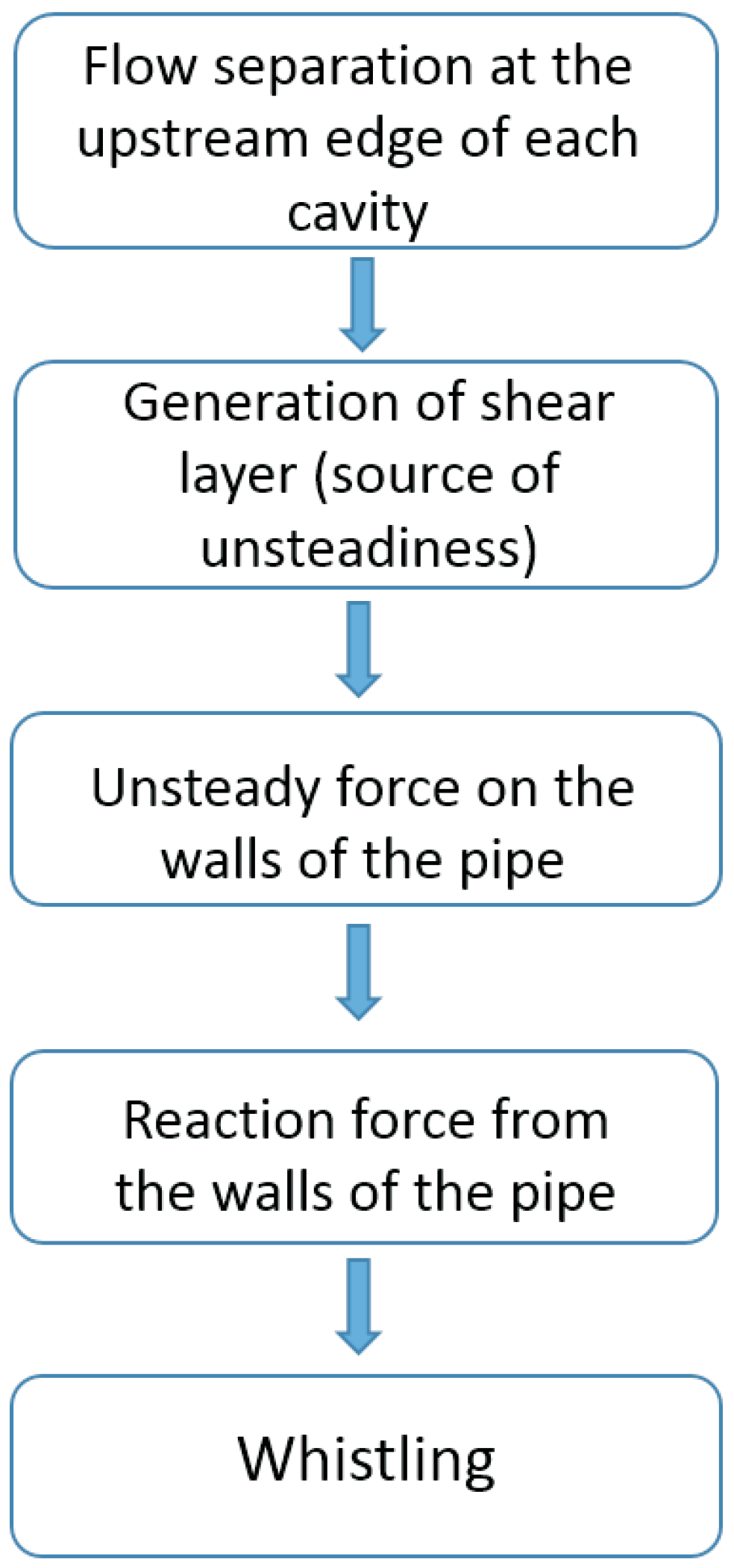
Sound generation in corrugated pipes is a result of an oscillation produced through a flow-acoustic interaction [6,7]. The generation of a shear layer is the result of flow separation taking place at the upstream edge of each cavity. This shear layer serves as a source of unsteadiness in the flow. Due to this unsteadiness, an unsteady force is being exerted on the walls. In response to this hydrodynamic force, the walls of the pipe exert a force that is basically considered as a source of sound, as shown in Figure 1 [8]. The flexibility of these pipes is not a prerequisite condition for generation of sound in them. However, the unsteady forces on the walls of the pipe thereby induce some mechanical vibrations that may have a significant effect [9]. The coupling of the shear layers with longitudinal acoustic waves in the pipe is the most commonly observed phenomenon [9,10,11,12]. The vortex shedding is controlled by the resulting high-amplitude oscillations [13,14]. These types of flow pulsations are referred to as self-sustained oscillations and result in high-amplitude sound generation, which is also called whistling. This whistling can consist of hydrodynamic and acoustic subsystems [9,15]. The instability of the shear layer, which is acting as an amplifier, is basically the hydrodynamic subsystem, and provides the system with acoustic energy. Acting as the acoustic subsystem are the longitudinal standing waves that act as a band-pass filter, which, in turn, is responsible for maintaining synchronization in this feedback mechanism. Because of this band-pass filter, there is a stepwise increment in the whistling frequency corresponding to certain flow velocities, as observed during various experimental studies [3,4,11,12,16,17,18].

In comparatively shorter whistling pipes displaying very strong acoustical reflections at their ends, the vortex shedding taking place at the upstream edge of the cavities is activated as a result of the oscillating velocity, which is associated with resonant longitudinal acoustical standing waves inside the pipe. The values of the acoustic passive resonance frequency of the pipe and the oscillating frequency will often be in close proximity to each other resulting in an acoustic pipe mode [19]. The combination of the vortex shedding occurring locally at the cavities and the longitudinal acoustic waves that travel along the pipe results in whistling inside corrugated pipes [2,15,17,20,21,22,23,24,25,26,27]. When the acoustic oscillations and the source of sound are synchronized with each other, this synchronization can be described in terms of a ratio of a convection time due to the vorticity perturbations across the cavity to the oscillation time period of the acoustic field. This ratio is most commonly regarded as the Strouhal number [19] and is given as

$$St=\frac{fW}{U_{corr}}$$

(1)

where f is the oscillation frequency, W is the cavity width, and $U_{corr}$ is the steady flow velocity in the corrugated pipe.

Tonon et al. [15] presented an experimental study comparing the whistling behavior of a pipe system with multiple side branches and a system consisted of corrugated pipes. They suggested that the multiple side branch system is an acceptable model for corrugated pipes. A captivating aspect of their study was that the system was found to whistle at the second hydrodynamic mode of the cavities rather than at the first. They proposed a prediction model for the whistling behavior that consisted of an energy balance, formulated on the basis of vortex sound theory.

Nakiboglu et al. [25] performed an investigative work regarding the whistling behaviors of two geometrically periodic systems, i.e., corrugated pipes and a multiple side branch system. In both systems, they observed a non-monotonic behavior in the whistling amplitude as a function of flow velocity, with local maxima corresponding to lock-in frequencies. In their effort to quantify the Strouhal number, they considered a variety of characteristic lengths. In their study, the shape of the upstream edge of the cavity also exhibited a significant effect on pressure fluctuation amplitudes for both corrugated pipes and the multiple side branch system [25]. They reported that the round upstream edges of the cavities increased the amplitude of the pressure fluctuation by up to five times in comparison to the sharp edges. Moreover, they found that the radius of the downstream edge did not have any considerable effect on the sound production. Using the same experimental setup, Nakiboglu et al. [26] studied the effects of the variation of different parameters on the whistling of corrugated pipes. They performed this study on corrugated pipe segments with different lengths and cavity geometries, and demonstrated that the peak-whistling Strouhal number, which is based on a characteristic length of the sum of the cavity width, and the upstream edge radius, was independent of the pipe length. They also indicated that the peak-whistling Strouhal number decreased with increasing confinement ratio, which was defined as the ratio of the pipe diameter to the sum of the cavity width and the upstream edge radius $D_p/(W+r_{up})$.

Nakiboglu et al. [27] conducted a study related to the aeroacoustics of a swinging corrugated tube. The main idea behind the work was that, when a short corrugated pipe segment is swung around one’s head, it tends to produce a musically intriguing whistling sound; this system was named the “Hummer”. Their experiments indicated that the Hummer could remain silent even when there was turbulence in the flow. Thus, they concluded that the absence of whistling was not in relation to a lack of turbulence. They anticipated that the reason for the absence of the fundamental mode in short corrugated pipes was the inability of the acoustic sources at the inlet and the outlet of the pipe to cooperate with each other, as a result of difference in their mean velocity profile.

Rudenko et al. [19] proposed a linear model for plane-wave propagation along a corrugated pipe. They considered an experiment in which a corrugated segment was placed between two smooth pipe segments, creating a system called a composite pipe. Their experiments assessed a quasi-steady model for convective acoustic losses which was dependent upon the pipe inlet geometry. Their model predicted some whistling modes that were not observed in the experiments. They reported that in various cases, they encountered a large overlap between the whistling ranges of successive modes, implying the domination of one mode and the suppression of the neighboring ones.

This paper discusses the results obtained through an experimental study performed using a combination of smooth and corrugated pipes. The pipe system under consideration consists of two smooth pipe segments attached to either end of a corrugated pipe segment. We performed experiments on different combinations of such pipe systems using various smooth and corrugated pipe lengths. The objective of this study is to analyze the effect of the variation in the lengths of corrugated and smooth pipe segments, while maintaining the same geometric specifications. For each pipe configuration, there exists a critical Mach number, $M_{cr}$, at which the system starts whistling. In our experiments, the Reynolds number, Re, was defined within the range of $6500\le$ Re $\le \mathrm{32,000}$, while the inner diameter of the smooth pipe (15.25 mm) was considered to be the characteristic length, and the kinematic viscosity of the working fluid (air) was $\nu =1.5\times {10}^{-5}$ m${}^2$/s.

In Section 2, we briefly describe vortex sound theory and explain the dimensionless parameters used. In Section 3, we describe the experimental set-up and procedure. We define the geometric specifications of the smooth and corrugated pipes used in our study and the considered pipe configurations. In Section 4, Section 5 and Section 6, we discuss the experimental results, and Section 7 provides the conclusion of this work.

2. Theoretical Background

2.1. Vortex Sound Theory

Vorticity as a source of sound can be demonstrated by considering the analogy provided by Howe [28,29,30], according to which an acoustical flow is basically the unsteady irrotational component of the total flow. Howe [29] used the decomposition of Helmholtz to divide the flow into rotational and irrotational parts for a given flow field $\mathbf{u}$:

$$\mathbf{u}=\nabla \varphi +\nabla \times \mathit{\psi }$$

(2)

where $\varphi$ is a scalar potential and $\mathit{\psi }$ is a vector stream function. Because the acoustical field should be a compressible and unsteady flow, the acoustical flow velocity ${\mathbf{u}}^{\prime }$ is defined as

$${\mathbf{u}}^{\prime }=\nabla {\varphi }^{\prime }$$

(3)

where ${\varphi }^{\prime }=\varphi -{\varphi }_0$ is the deviation of $\varphi$ from the steady component ${\varphi }_0$ of the potential. Since the flows with low Mach numbers and high Reynolds numbers are being dealt with here, heat transfer and friction can be neglected. Thus, for a homentropic flow, an explicit relation between vorticity and sound production is obtained using Crocco’s formulation for the momentum equation [15]:

$$\frac{\overline{\partial \mathbf{u}}}{\partial t}+\nabla B=-\mathit{\omega }\times \mathbf{u}$$

(4)

where $B=\frac{1}{2}\left|{\mathbf{u}}^2\right|+\int \frac{dp}{\rho }$ is the total enthalpy and $\mathit{\omega }=\nabla \times \mathbf{u}$ is the vorticity. At low Mach numbers, the convective effects on sound wave propagation can be neglected, which results in the following relation [15],

$$\frac{1}{c_0^2}\frac{{\partial }^{2}B}{\partial t^2}-{\nabla }^{2}B=\nabla ·(\mathit{\omega }\times \mathbf{u})$$

(5)

In Equation (5), the right-hand side corresponds to the assumption that the Coriolis force density ${\mathbf{f}}_{coriolis}=-{\rho }_0(\mathit{\omega }\times \mathbf{u})$, where ${\rho }_0$ is the fluid density, acts as the source of sound.

According to Howe [29], the time-averaged acoustic source power $<P_{source}>$ can be estimated as

$$<P_{source}>=-{\rho }_0<{\int }_V(\mathit{\omega }\times \mathbf{u})·{\mathbf{u}}^{\prime }dV>,$$

(6)

where V is the volume in which $\mathit{\omega }$ is not vanishing and the brackets $<\cdots >$ indicate time averaging.

2.2. Dimensional Parameters

The centre-line velocity $U_{cl}$ relates the average velocity inside a smooth pipe $U_{sp}$ by the empirical relation [31]

$$U_{sp}\simeq U_{cl}/(1+1.33\sqrt{F}),$$

(7)

where the friction factor F for a smooth pipe is given by the formula of Blasius [31]:

$$F\simeq 0.316R{e}^{-0.25}.$$

(8)

For the Reynolds number considered in our experiments, we approximate the smooth pipe velocity as $U_{sp}\simeq U_{cl}/1.22$. Because of the slight difference between the smooth and corrugated pipe diameters, the average velocity inside the corrugated pipe is

$$U_{corr}=\frac{U_{sp}{D}_{sp}}{D_{corr}},$$

(9)

where $U_{corr}$ is the average velocity in corrugated segment, $D_{sp}$ is the smooth pipe diameter, and $D_{corr}$ is the corrugated pipe diameter. Thus,

$$U_{corr}\simeq U_{cl}/\alpha ,\alpha =1.32.$$

(10)

Therefore, the steady cross-sectional average velocity inside the corrugated pipe is approximately 1.32 times lower than the centre-line velocity at the end of the downstream smooth pipe.

The Mach number (M) was calculated as

$$M=\frac{U_{cl}}{c_0},$$

(11)

where $c_0$ is the speed of sound in air at room temperature, which is equal to 340 m/s. Moreover, the Helmholtz Number was calculated as

$$He=\frac{Lf}{c_0}=\frac{LS{t}_{cr}}{\alpha W}M,$$

(12)

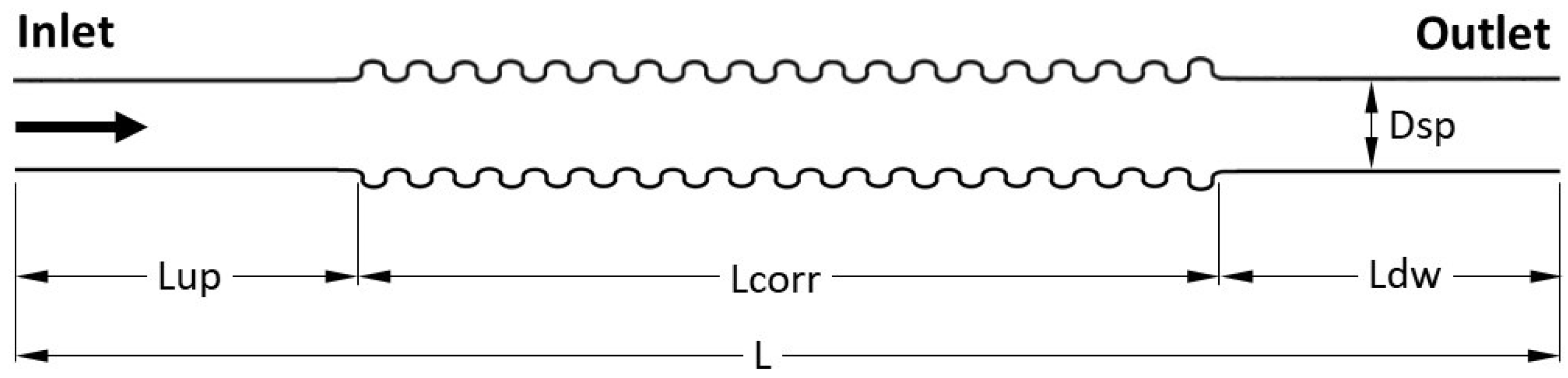
where $L=L_{up}+L_{corr}+L_{dw}$ is the sum of the lengths of all three pipes considered in each configuration, as can be seen in Figure 2; f is the whistling frequency in Hz; $S{t}_{cr}$ is the critical Strouhal number at which the whistling begins; and W is the cavity width.

3. Design of Model Experiment (Set-Up and Procedure)

3.1. Test Model and Corrugated Pipe System Configurations

The pipe system consists of three pipe segments, as shown in Figure 2. The first segment is the upstream smooth pipe segment $L_{up}$ and is followed by the corrugated tube $L_{corr}$ and the downstream smooth segment $L_{dw}$. The smooth pipe segments are made of aluminium. The inner diameter of the smooth pipes is 15.25 mm, and their thickness is 4.75 mm. The corrugated pipe segment is made of plastic.

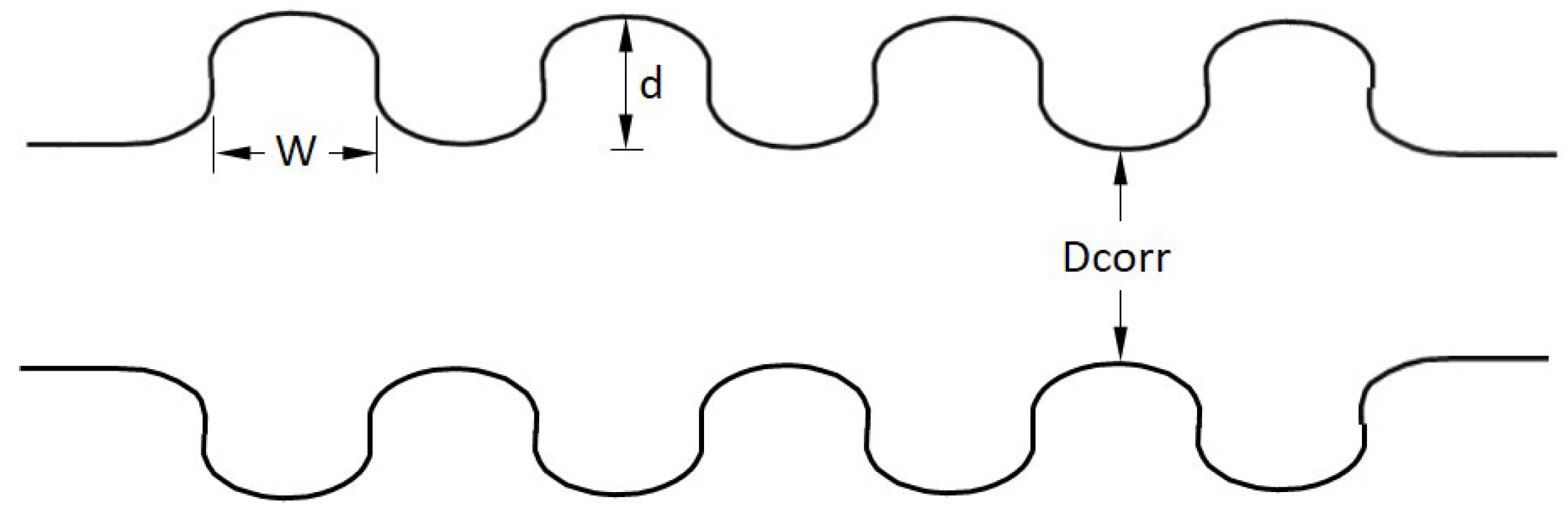
Figure 3 shows the corrugated pipe geometry (drawn not to scale). The inner diameter $D_{corr}$ is 16.5 mm, the depth d of the cavities is estimated to be 1.3 mm, and the width W is 2.3 mm. Three different lengths of corrugated pipes, 250, 350, and 450 mm, were used. The smooth pipes used in the experiment had lengths of 100, 200, 300, and 400 mm.

Table 1. Various combinations of smooth and corrugated pipes categorized into two cases. Case a refers to the three different $L_{corr}$ values (250, 350, and 450 mm) for one $L_{up}$ value (100 mm) and four $L_{dw}$ values (100, 200, 300 and 400 mm). Case b corresponds to the same three $L_{corr}$ values for one $L_{dw}$ value (100 mm) and four $L_{up}$ values (100, 200, 300 and 400 mm).

Case a	${\mathit{L}}_{\mathit{up}}$ (mm)	${\mathit{L}}_{\mathit{corr}}$ (mm)	${\mathit{L}}_{\mathit{dw}}$ (mm)	Case b	${\mathit{L}}_{\mathit{up}}$ (mm)	${\mathit{L}}_{\mathit{corr}}$ (mm)	${\mathit{L}}_{\mathit{dw}}$ (mm)
I	100	250	100–400	I	100–400	250	100
II		350		II		350
III		450		III		450

shows the details of all pipe system configurations considered in this study.

Experiments were performed with various combinations of smooth and corrugated pipe segments in an on-coming inlet flow, which is considered to be a uniform flow because the inlet end pipe is directly connected to the wind tunnel contraction area. Each corrugated pipe was tested with all four lengths of smooth pipes first at the downstream and then at the upstream end. The pipe configurations were divided into two cases, which are described as follows.

• Case a: $L_{dw}\ge L_{up}$. The length of the downstream smooth pipe was equal to or greater than the length of the upstream smooth pipe.
• Case b: $L_{dw}\le L_{up}$. The length of the downstream smooth pipe was equal to or less than the length of the upstream smooth pipe.

3.2. Test Equipment and Measurement Procedure

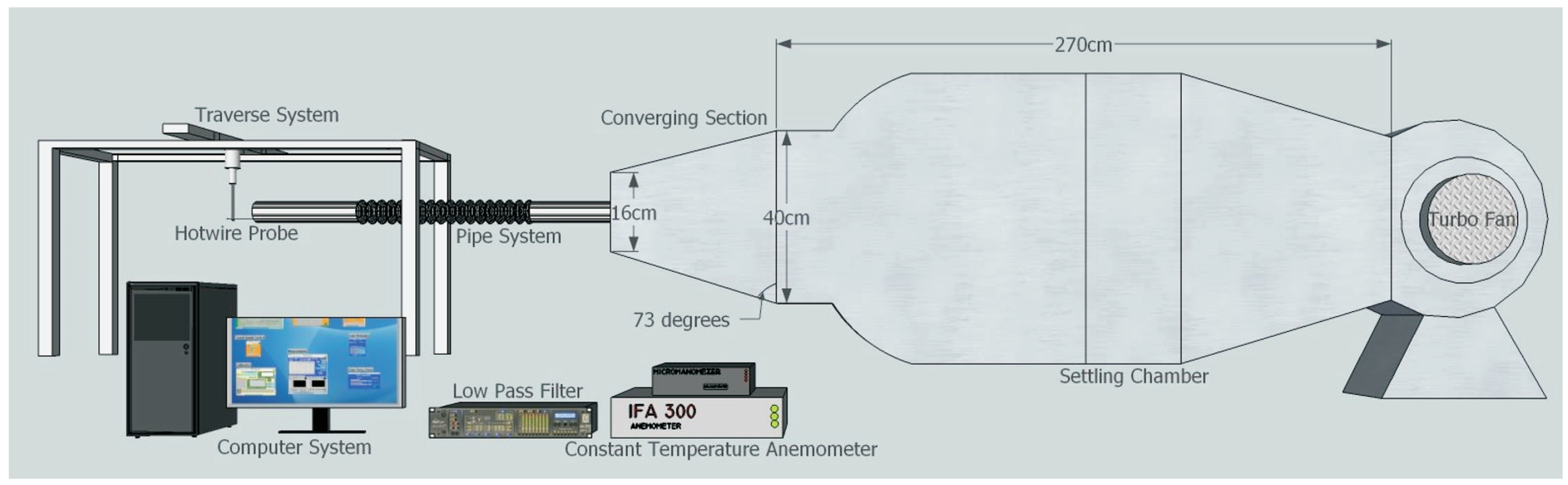
Figure 4 shows a three-dimensional (3D) sketch of our experimental set-up. The set-up consists of a wind tunnel as the primary source of high-velocity air with a settling chamber installed. A 5-cm-thick layer of acoustic absorbing material was attached to the side walls of the settling chamber to avoid acoustic resonance in the settling chamber. The length of the wind tunnel is 270 cm, and the discharge flange has an outer cross section of 50 cm × 50 cm and an inner cross section of 40 cm × 40 cm. The air is generated by a Turbo Fan with a volumetric air flow of 250 m${}^3$/min, a total pressure of 800 mmAq, and a rated power of 7.5 kW, thus ensuring a uniform inflow condition at the upstream end of the pipe system. The air from the wind tunnel is passed through the pipe system by connecting a converging section at the end of the tunnel. The dimensions of the section are such that the upstream end had a cross section of 40 cm × 40 cm, whereas the downstream end cross section was 16 cm × 16 cm. A straight miniature wire probe (55P11) was fixed inside the pipe on the pipe axis (between the centre and the pipe wall) a few millimeters upstream from the downstream open pipe end by means of a probe support. Miniature wire probes have platinum-plated tungsten wire sensors with a diameter of 5 $\mathsf{\mu }$m and a length of 1.25 mm. The probe body is a 1.9 mm diameter ceramic tube, equipped with gold-plated connector pins that connect to the probe supports by plug-and-socket arrangements. The output of the probe support was attached to an IFA 300 constant temperature anemometer system. It provides a frequency response of up to 300 kHz, depending on the sensor used. The output of the anemometer system was sent to a low-pass filter (dual channel programmable filter 3624, NF Corporation) for signal conditioning. In the HW measurement, the sampling rate for data acquisition was 20 kHz, while the range of low-pass filter was 10 kHz taking the Nyquist criterion into account. After being filtered, the signal was sent to the computer via a National Instruments data acquisition board. A pitot tube was also coaxially attached to the hotwire probe support by a clamping mechanism at the downstream pipe outlet to measure the free stream air velocity. The velocity was measured using an FC012-Micromanometer. National Instruments LabVIEW software was used for data processing and analysis. The calibrated hot wire provided a measurement of the time-dependent velocity at the axis of the pipe. Using the spectrum analysis in LabVIEW, we obtained the frequency peaks at which the whistling sound occurred.

4. Effect of Downstream Smooth Pipe Length on the Whistling Behavior for Constant Corrugated Segment Length (Case a)

4.1. Shortest Corrugated Segment: Case a-I ($L_{corr}/D_{corr}=$ 15.2)

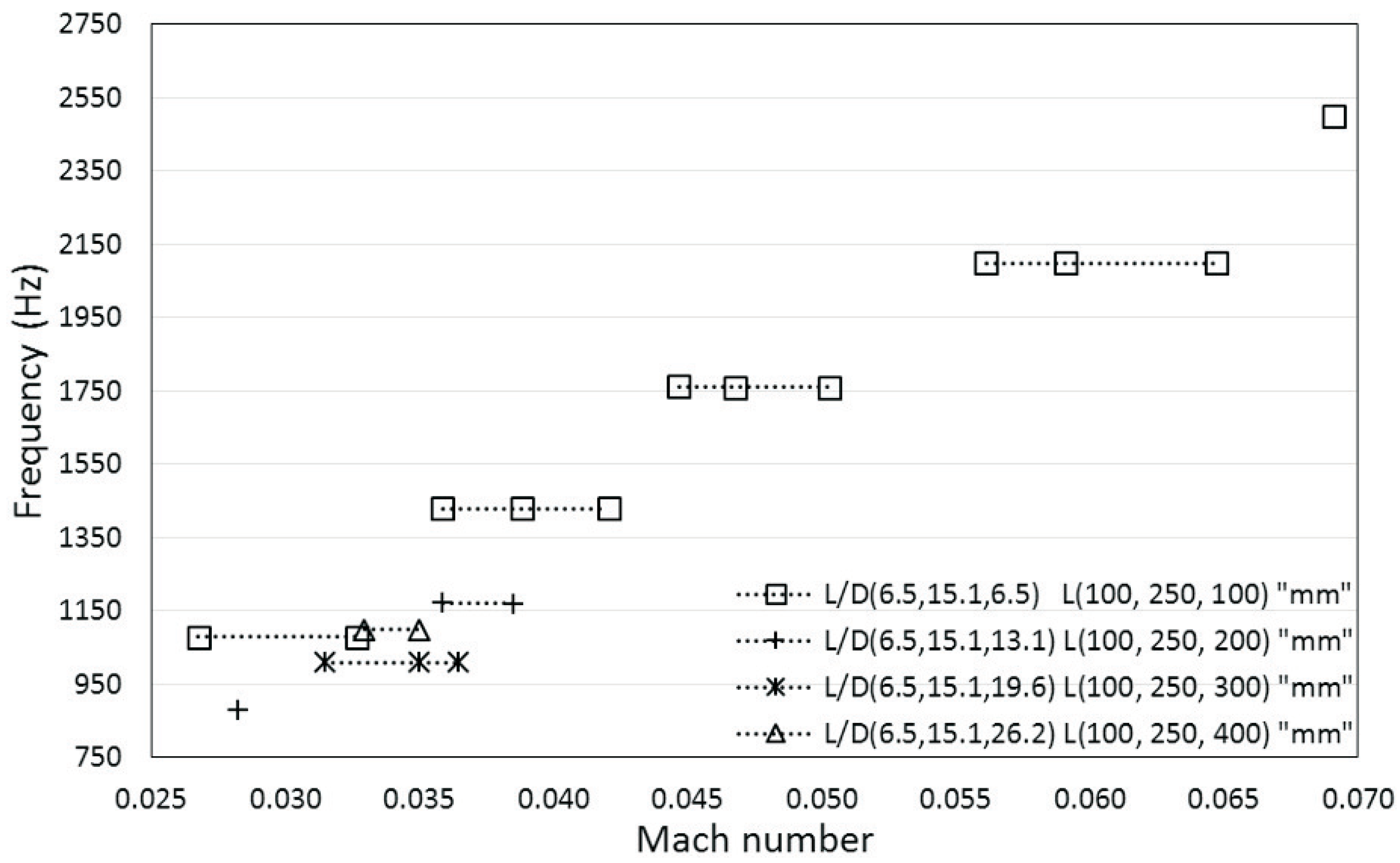
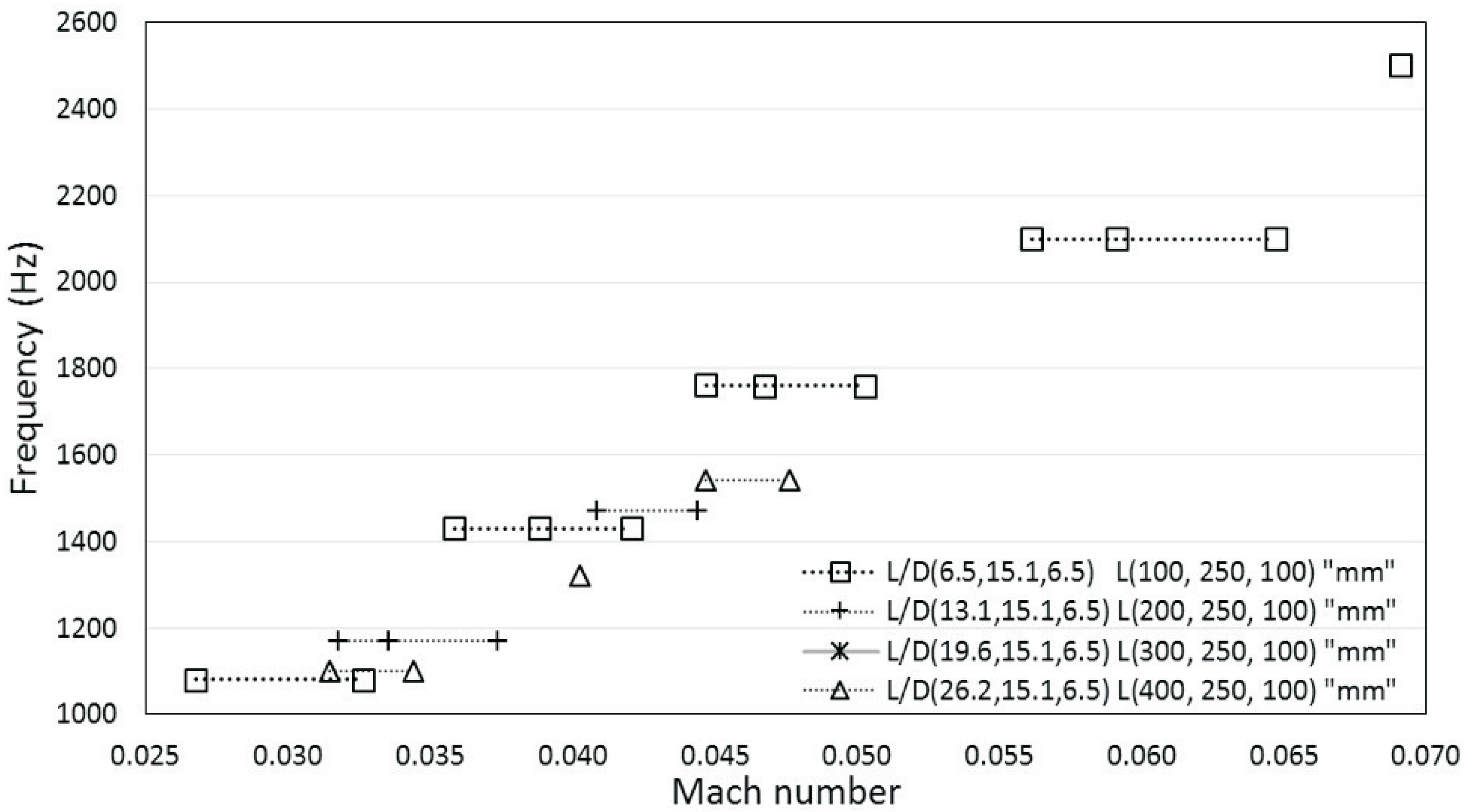
With increasing corrugated segment length, the pipe systems for all smooth pipe lengths, both upstream and downstream, tend to whistle at higher frequencies and Mach numbers. For the corrugated pipe with a length of 250 mm (Case a-I), when the length of the downstream smooth pipe was increased from 100 to 400 mm at intervals of 100 mm, the frequency and Mach number range within which whistling occurred decreased, as shown in Figure 5 and

Table 2. Mach number and corresponding frequency range (Hz) for pipe systems in Case a-I.

${\mathit{L}}_{\mathit{up}}$ (mm)	${\mathit{L}}_{\mathit{corr}}$ (mm)	${\mathit{L}}_{\mathit{dw}}$ (mm)	Mach Number Range	Corresponding Frequency Range (Hz)
100	250	100	0.027–0.069	1080–2500
		200	0.028–0.039	880–1170
		300	0.031–0.036	1010
		400	0.033–0.035	1100

. The maximum whistling range was observed for equal upstream and downstream pipe lengths of 100 mm. This pipe system whistled at Mach numbers ranging from M = 0.027 to 0.069 and with frequencies from 1080 to 2500 Hz, which respectively correspond with the minimum and maximum Mach numbers in the range. Maintaining a fixed upstream pipe length of 100 mm, when $L_{dw}=200$ mm, a drastic decrement in the whistling range was observed. The pipe system whistled from M = 0.028 to 0.039, corresponding to frequencies of 880 and 1170 Hz, respectively. Pipe systems with a downstream pipe of 300 mm in length resulted in further reduction in whistling ranges; whistling occurred from M = 0.031 to 0.036 at a constant frequency of 1010 Hz. Finally, for the downstream smooth pipe with a length of 400 mm, the pipe system whistled very briefly at a frequency of 1100 Hz from M = 0.033 to 0.035.

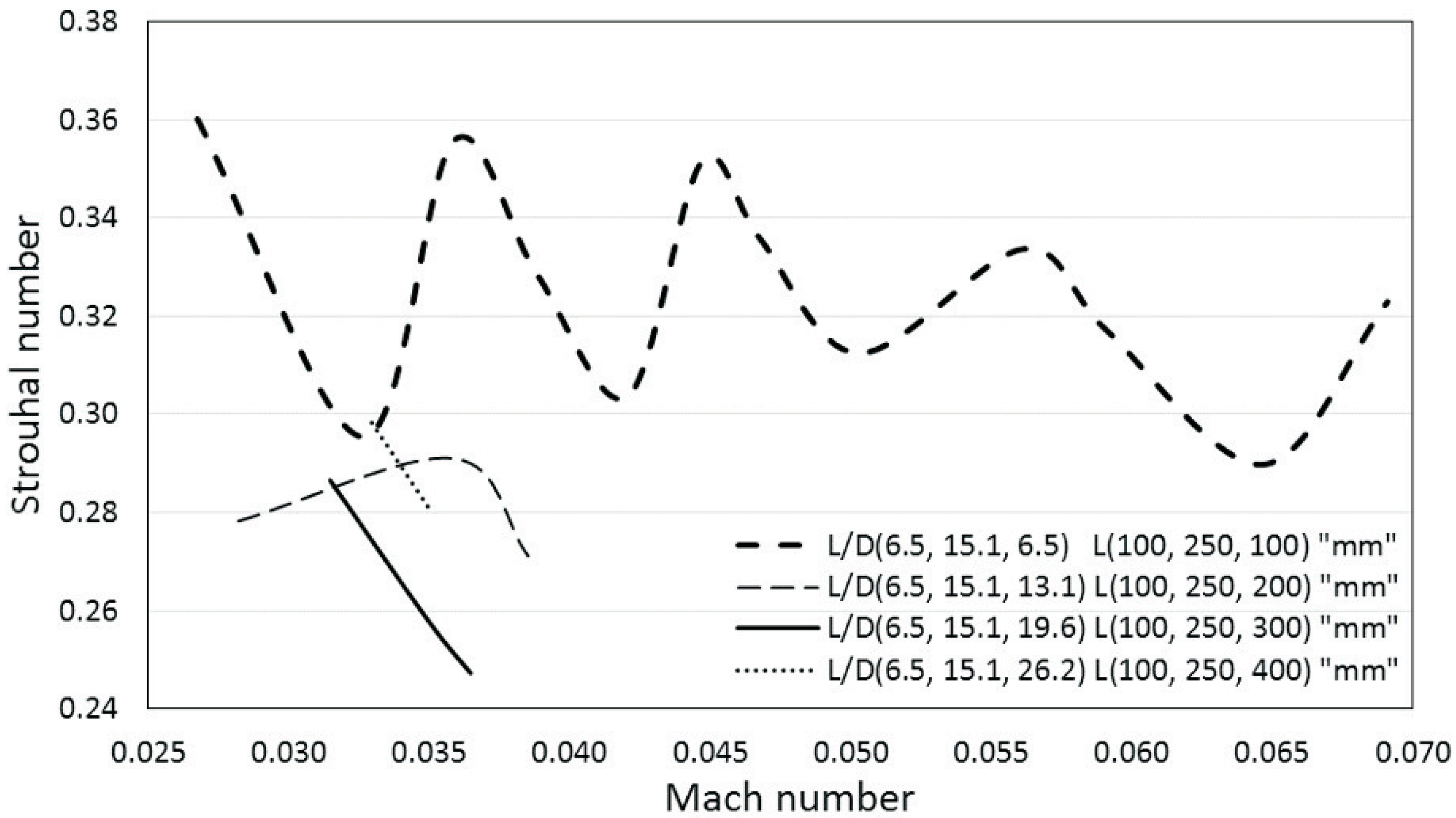
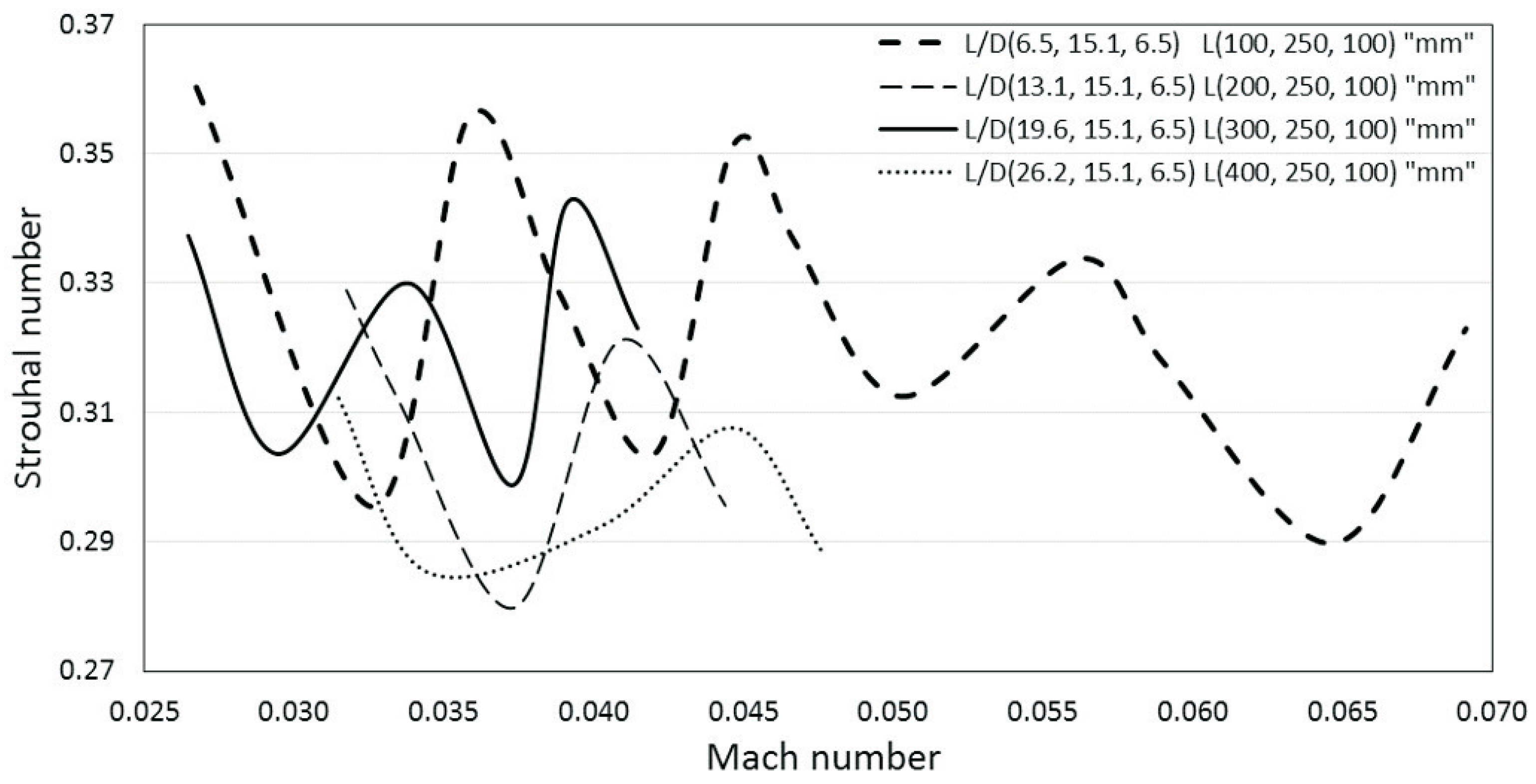
Unlike frequency, the Strouhal number does not increase linearly with the Mach number but instead shows fluctuating behavior. For $L_{dw}=100$ mm, the initial and final Strouhal numbers at M = 0.027 and 0.067 were 0.36 and 0.32, respectively. The Strouhal and Mach number ranges were the broadest of all pipe systems considered in Case a-I, as can be seen in Figure 6 and

Table 3. Mach number range, corresponding Strouhal number ($St$) range and maximum Strouhal number for each pipe configuration in Case a-I.

${\mathit{L}}_{\mathit{up}}$ (mm)	${\mathit{L}}_{\mathit{corr}}$ (mm)	${\mathit{L}}_{\mathit{dw}}$ (mm)	Mach Number Range	Corresponding St Range	Max. St
100	250	100	0.027–0.069	0.36–0.32	0.36
		200	0.028–0.039	0.28–0.27	0.29
		300	0.031–0.036	0.29–0.25	0.29
		400	0.033–0.035	0.30–0.28	0.30

, with 0.36 as the highest Strouhal number in the Mach number range. For $L_{dw}=200$ mm, the range was significantly reduced; the Strouhal numbers are estimated to be 0.28 and 0.27 at M = 0.028 and 0.039, respectively, with a maximum Strouhal number of 0.29 in this range. For the downstream smooth pipe with a length of 300 mm, the starting Strouhal number was 0.29 at M = 0.031, and the ending Strouhal number was 0.25 at M = 0.036, with a maximum Strouhal number of 0.29 in this case. For $L_{dw}=400$ mm, the longest downstream smooth pipe considered in this study, the Mach numbers of M = 0.033 and 0.035 yielded Strouhal numbers of 0.30 and 0.28, respectively, with 0.30 as the highest Strouhal number in the range.

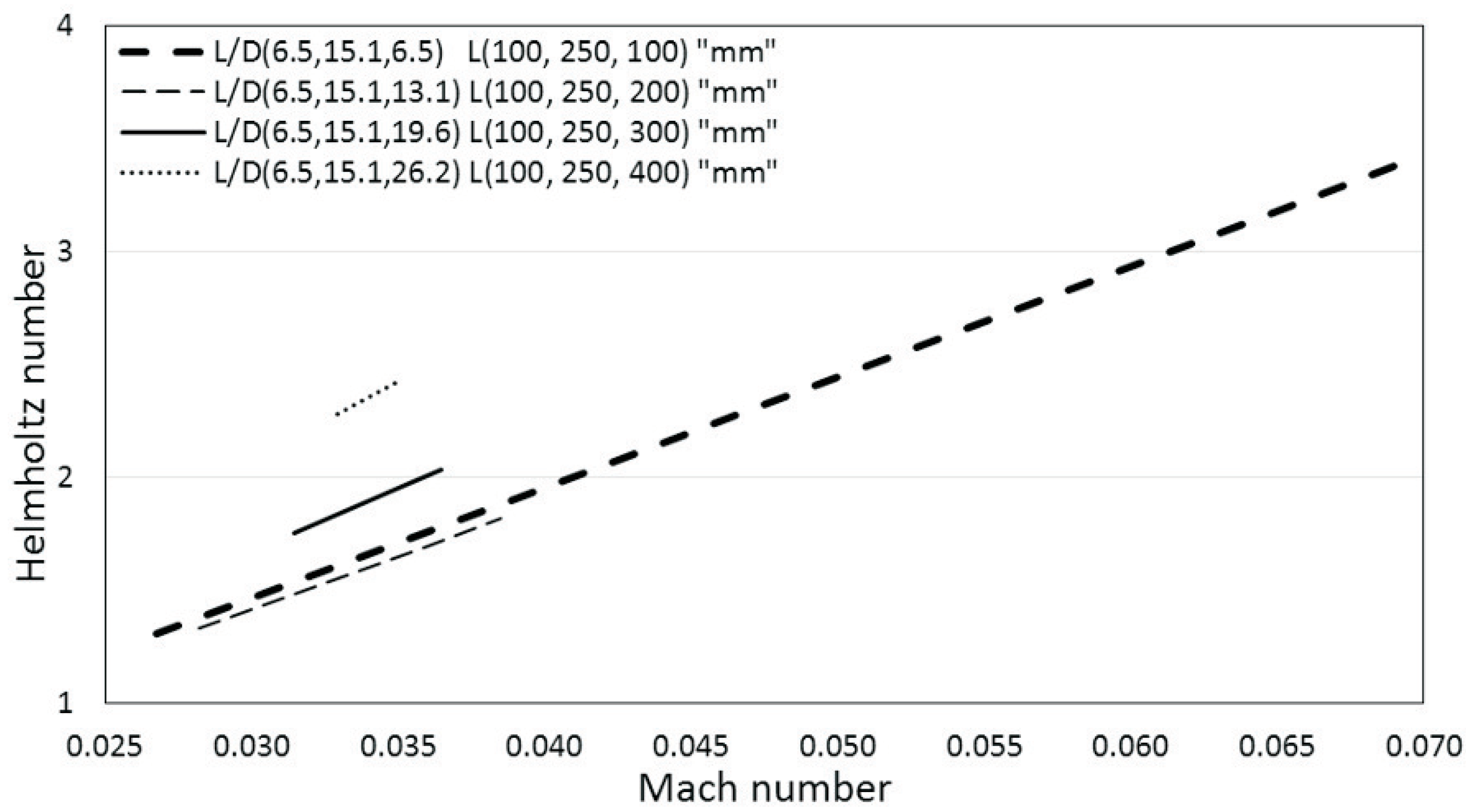
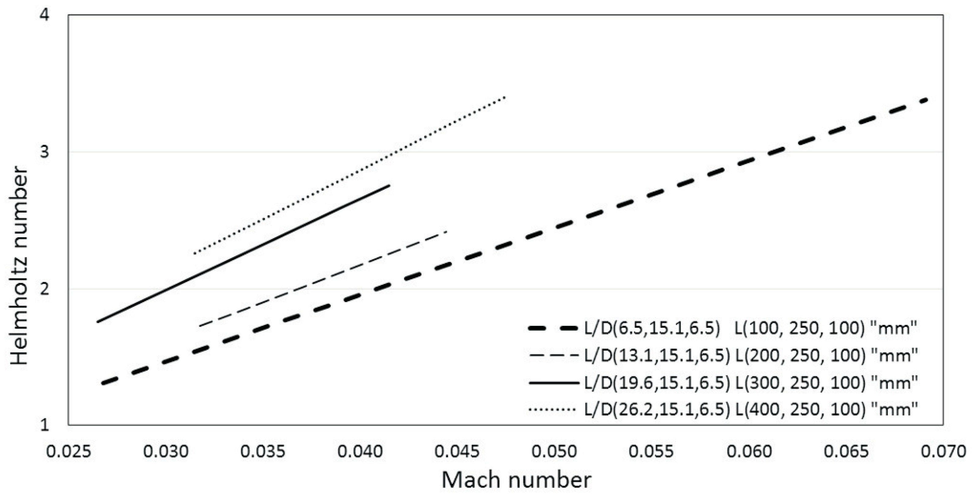
Similar to frequency, the Helmholtz number $He$ is linearly related to the Mach number. For the smallest downstream pipe, with a length of 100 mm, the minimum $He$ was 1.31 at M = 0.027, whereas the maximum $He$ was 3.38 at M = 0.067, as shown in Figure 7 and

Table 4. Mach number and corresponding Helmholtz number ($He$) range for pipe systems in Case a-I.

${\mathit{L}}_{\mathit{up}}$ (mm)	${\mathit{L}}_{\mathit{corr}}$ (mm)	${\mathit{L}}_{\mathit{dw}}$ (mm)	Mach Number Range	Corresponding He Range
100	250	100	0.027–0.069	1.31–3.38
		200	0.028–0.039	1.33–1.81
		300	0.031–0.036	1.75–2.03
		400	0.033–0.035	2.28–2.42

. For $L_{dw}=200$ mm, the minimum and maximum $He$ were 1.33 and 1.81 at M = 0.028 and 0.039, respectively. The minimum and maximum $He$ for $L_{dw}=300$ mm were 1.75 and 2.03 at M = 0.031 and 0.033, respectively. For the longest downstream smooth pipe of 400 mm, the minimum $He$, which occurred at M = 0.033, was 2.28, whereas the maximum $He$ occurred at M = 0.035 and was 2.42. This trend suggests that the range of $He$ with respect to M continuously shrinks as the length of the downstream smooth pipe increases.

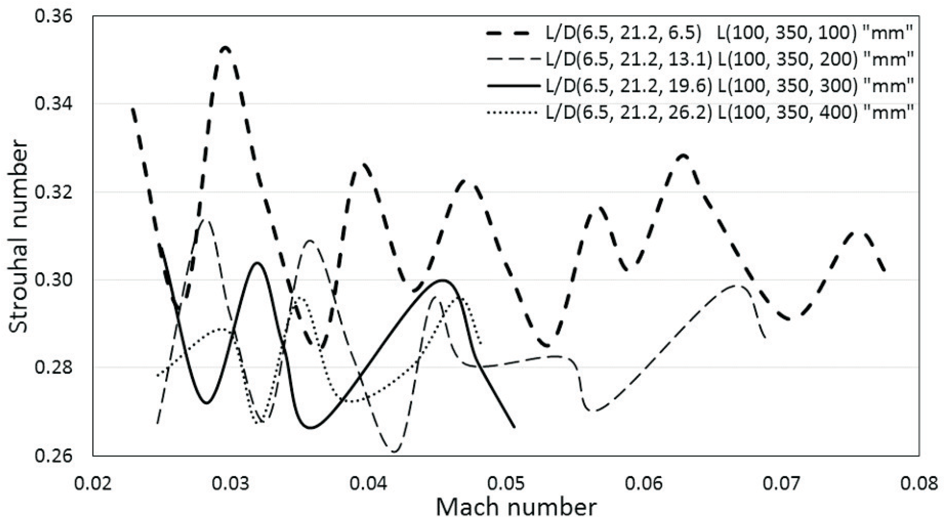
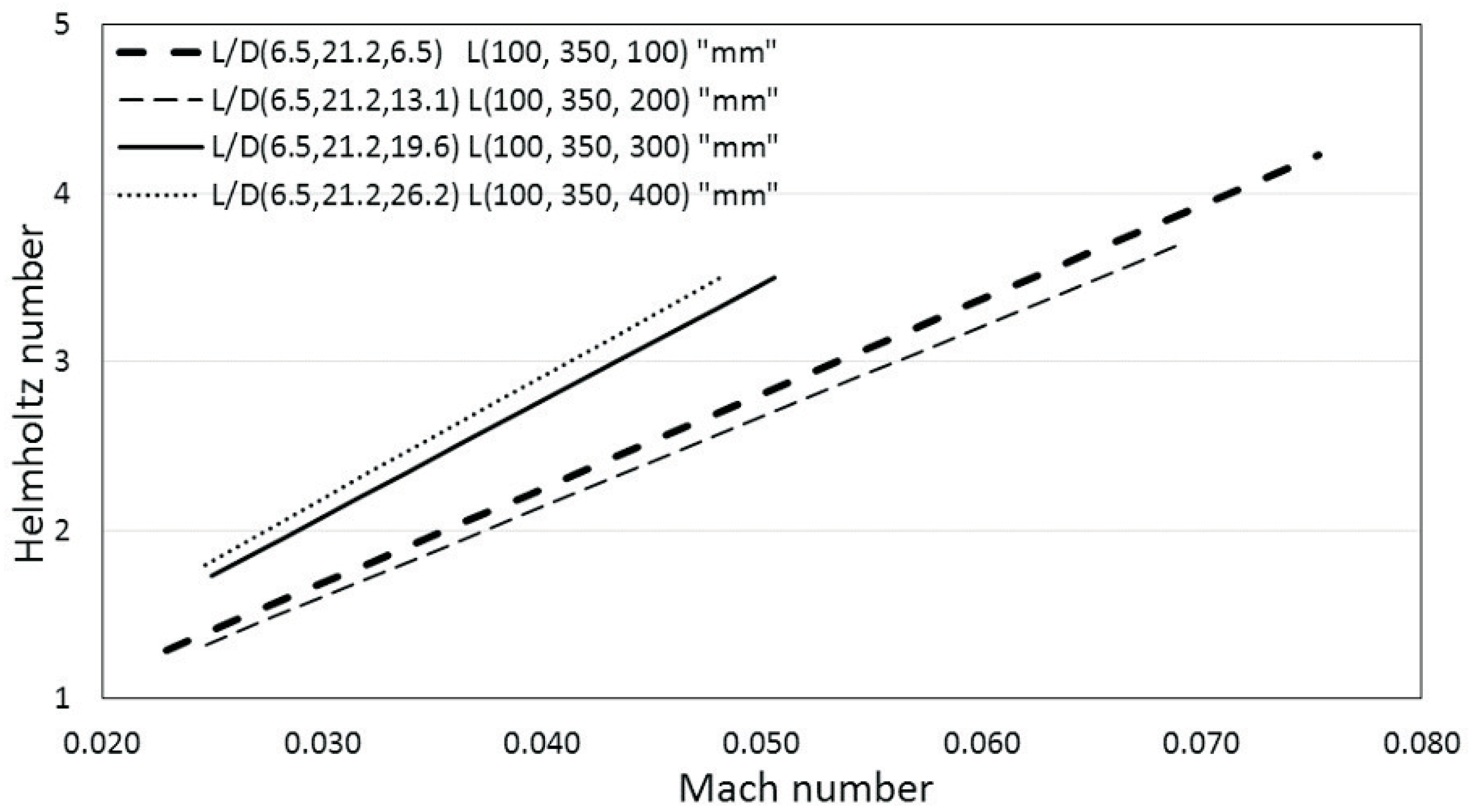
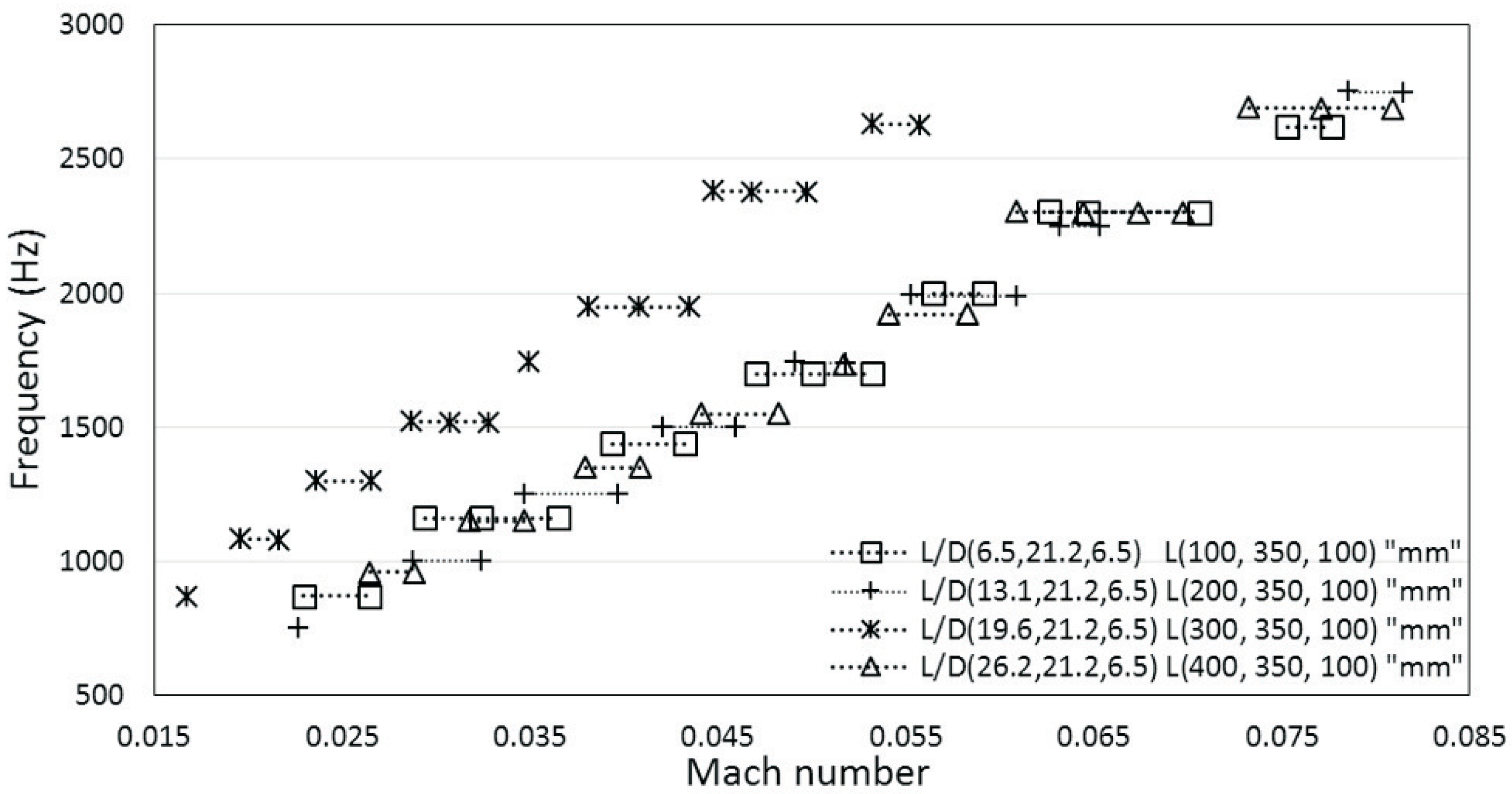
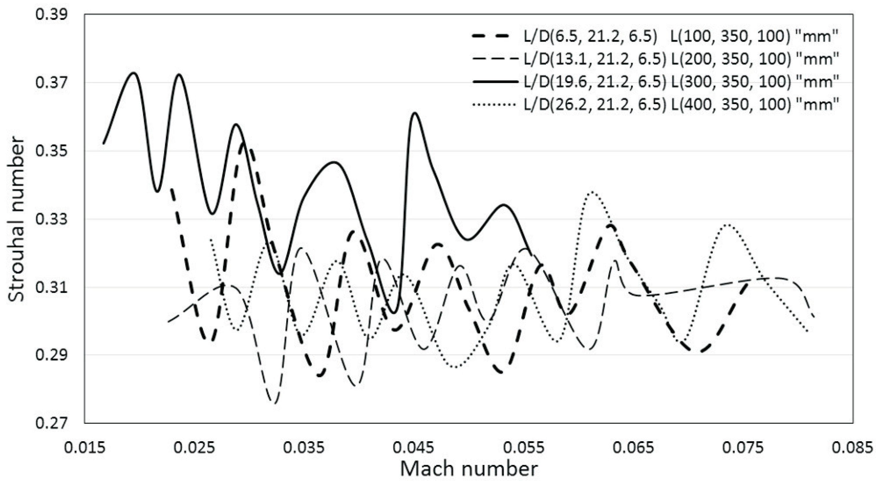
4.2. Intermediate Corrugated Segment: Case a-II ($L_{corr}/D_{corr}=$ 21.2)

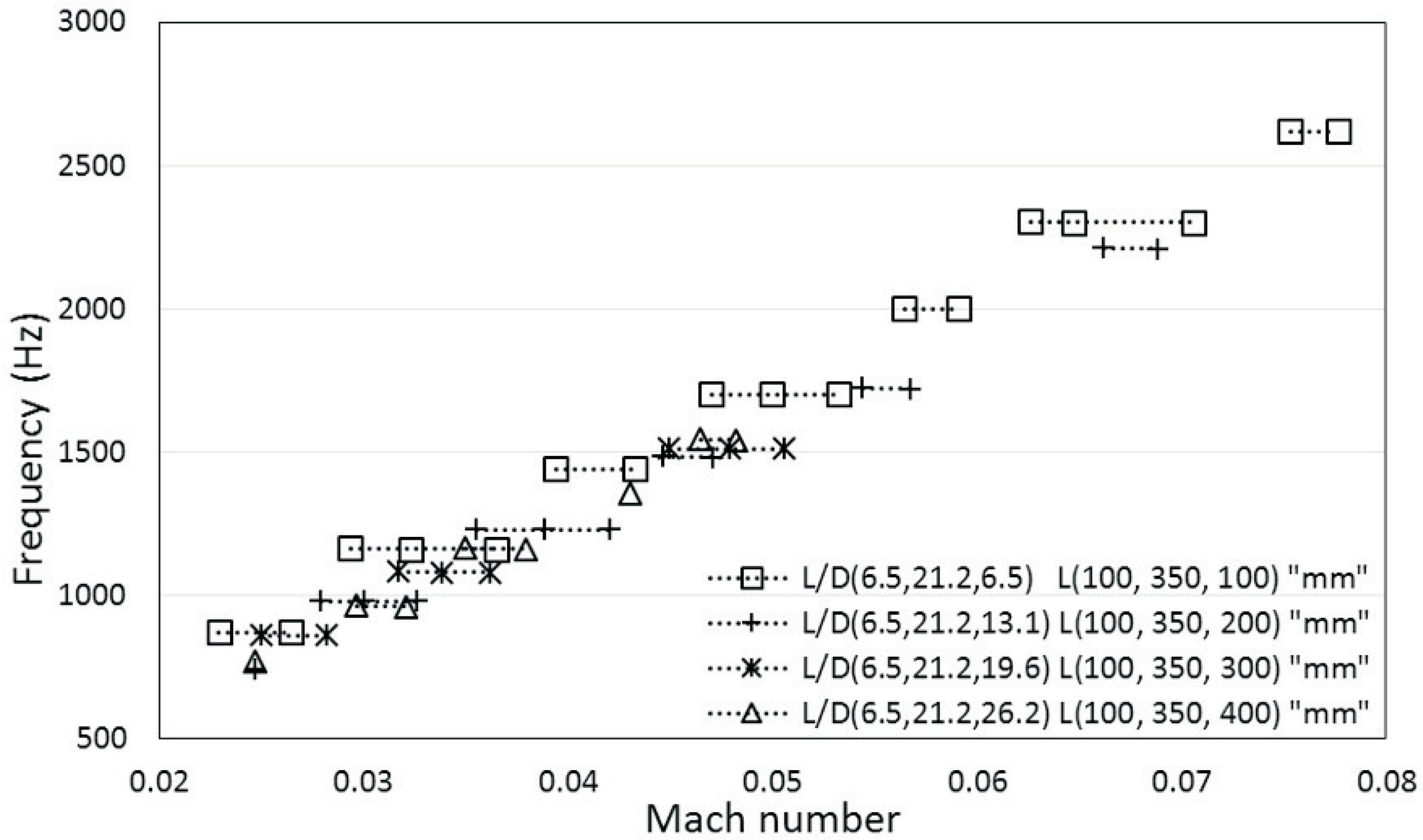
The next pipe system is Case a-II, which has a corrugated segment of length $L_{corr}=350$ mm, as shown in Figure 8. With $L_{up}=L_{dw}=100$ mm, the minimum and maximum Mach numbers were estimated to be 0.023 and 0.078, respectively, corresponding to a whistling frequency range of 870–2600 Hz. For $L_{dw}=200$ mm, the minimum and maximum Mach numbers were 0.025 and 0.069 with corresponding whistling frequencies of 750 and 2200 Hz, respectively. For $L_{dw}=300$ mm, the onset of whistling occurred at $M=$ 0.025 with a frequency of 850 Hz, and the pipe system whistled up to M = 0.051 with a frequency of 1500 Hz. Finally, for the downstream pipe with a length of 400 mm, whistling occurred from M = 0.025 to M = 0.048 with frequencies between 750 and 1550 Hz.

For $L_{dw}=100$ mm, the Strouhal number at a Mach number of 0.023, where whistling began, was 0.34, and at the maximum Mach number of 0.078, it was 0.30; the maximum Strouhal number within the whistling range was 0.35, as shown in Figure 9 and

Table 5. Mach number range, corresponding Strouhal number ($St$) range and maximum Strouhal number for each pipe configuration in Case a-II.

${\mathit{L}}_{\mathit{up}}$ (mm)	${\mathit{L}}_{\mathit{corr}}$ (mm)	${\mathit{L}}_{\mathit{dw}}$ (mm)	Mach Number Range	Corresponding St Range	Max. St
100	350	100	0.023–0.078	0.34–0.30	0.35
		200	0.025–0.069	0.27–0.29	0.31
		300	0.025–0.051	0.31–0.27	0.31
		400	0.025–0.048	0.28–0.29	0.30

.

For the downstream pipe length of 200 mm, the range of Mach numbers was 0.025–0.069, corresponding to Strouhal numbers of 0.27 and 0.29, respectively, with a maximum Strouhal number of 0.31. For $L_{dw}=300$ mm, the Strouhal number started at 0.31 and ended at 0.27 for M = 0.025 and 0.051, respectively, with a maximum Strouhal number of 0.31. Finally, for the downstream smooth pipe of length 400 mm, the starting and ending Strouhal numbers were 0.28 and 0.29 at Mach numbers of M = 0.025 and 0.048, respectively, with a maximum Strouhal number of 0.30.

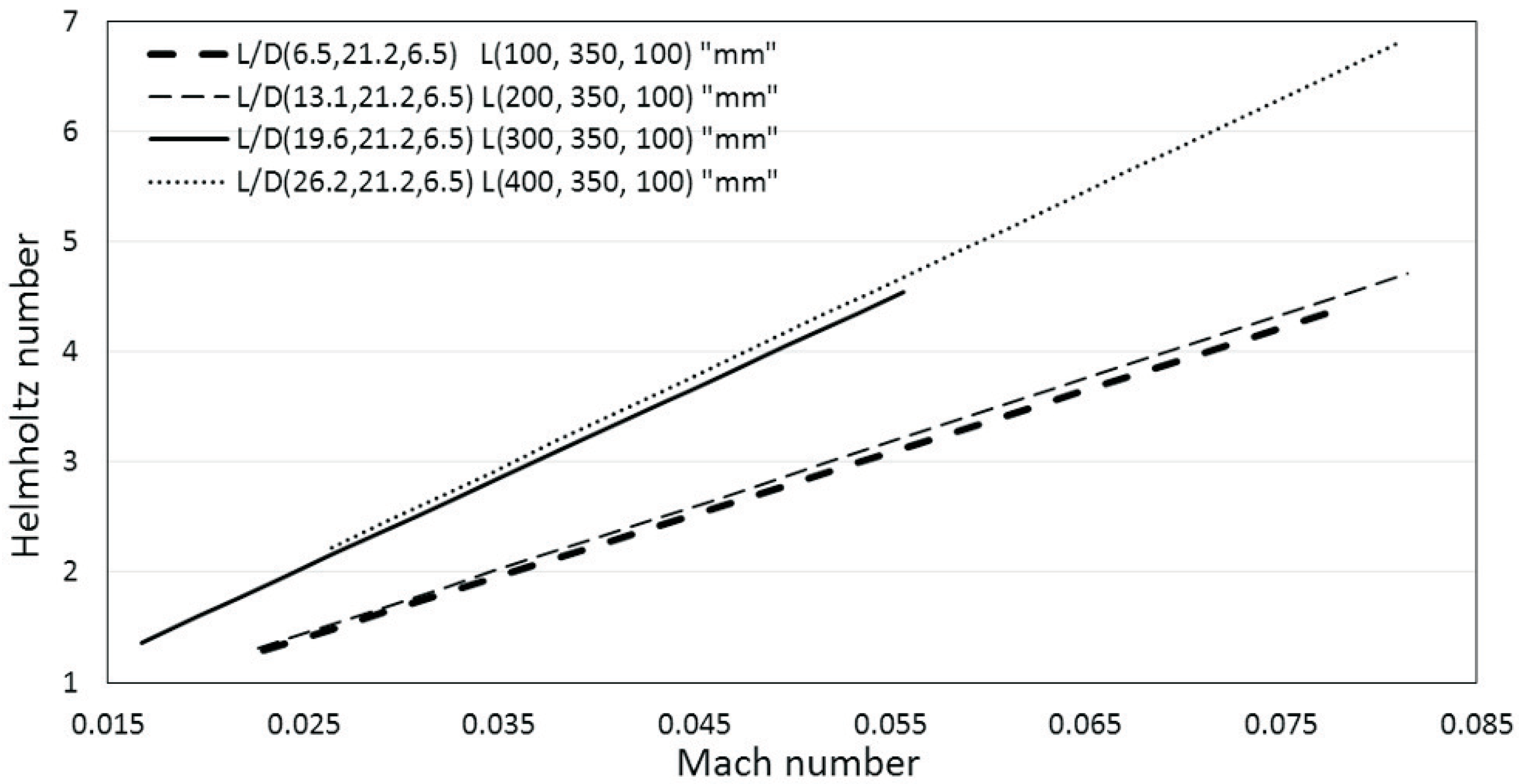
As shown in Figure 10 and

Table 6. Mach number and corresponding Helmholtz number ($He$) range for pipe systems in Case a-II.

${\mathit{L}}_{\mathit{up}}$ (mm)	${\mathit{L}}_{\mathit{corr}}$ (mm)	${\mathit{L}}_{\mathit{dw}}$ (mm)	Mach Number Range	Corresponding He Range
100	350	100	0.023–0.078	1.29–4.36
		200	0.025–0.069	1.32–3.68
		300	0.025–0.051	1.73–3.50
		400	0.025–0.048	1.80–3.51

, for the smallest downstream pipe of length 100 mm, the minimum Helmholtz number $He$ is 1.29 and occurs at M = 0.023, whereas the maximum $He$ is 4.36 at M = 0.078. For $L_{dw}=200$ mm, the minimum and maximum $He$ are 1.32 and 3.68 and occur at M = 0.025 and 0.069, respectively. The minimum and maximum $He$ for $L_{dw}=300$ mm are 1.73 and 3.50 at M = 0.025 and 0.051, respectively. For the longest downstream smooth pipe of length 400 mm, the minimum $He$ at M = 0.025 is reported to be 1.80, whereas the maximum $He$ at M = 0.048 is found to be 3.51. Thus this case has shown the similar behavior as Case a-I; increasing downstream smooth pipe length consistently decreased the range of Helmholtz number.

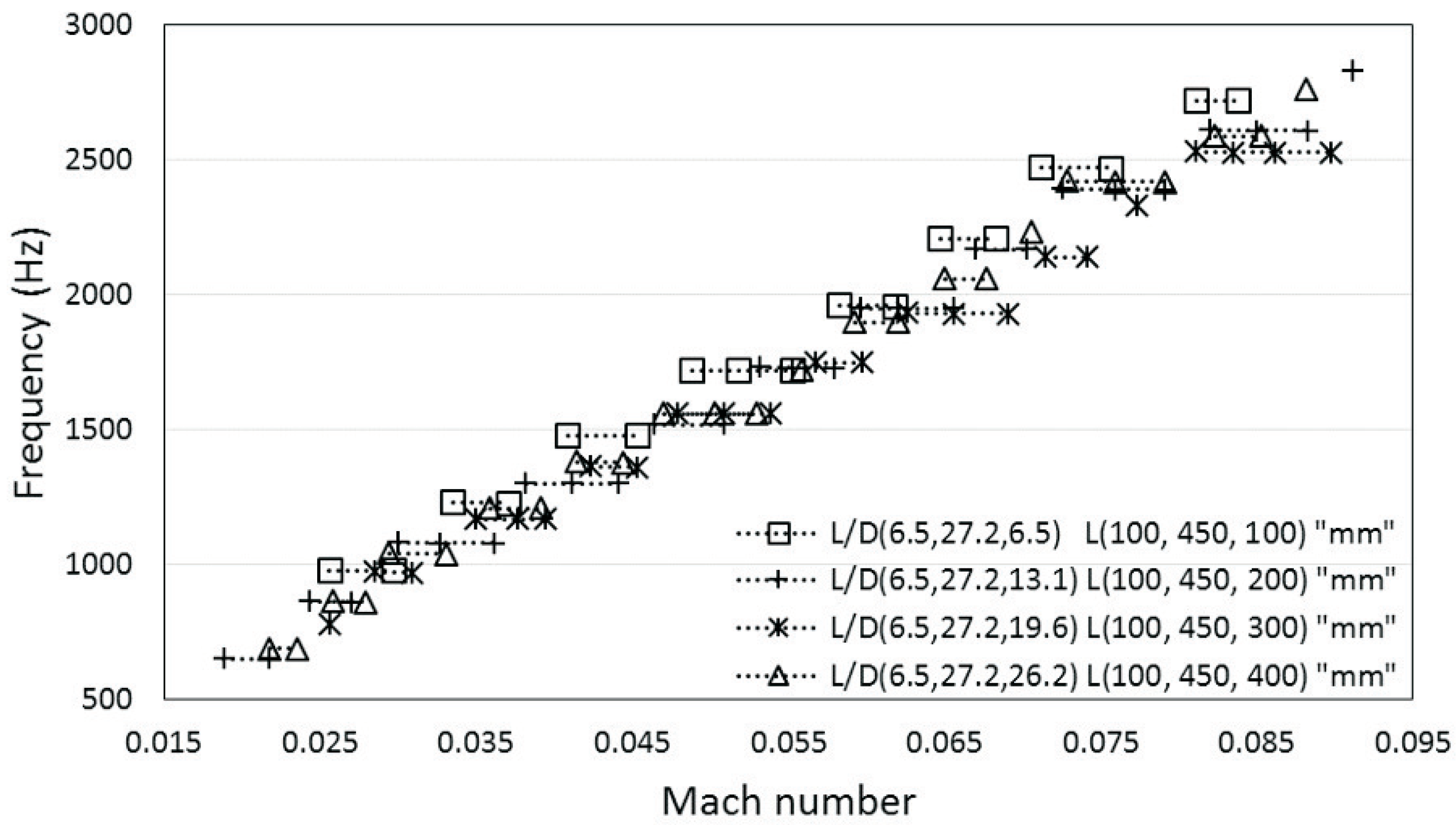
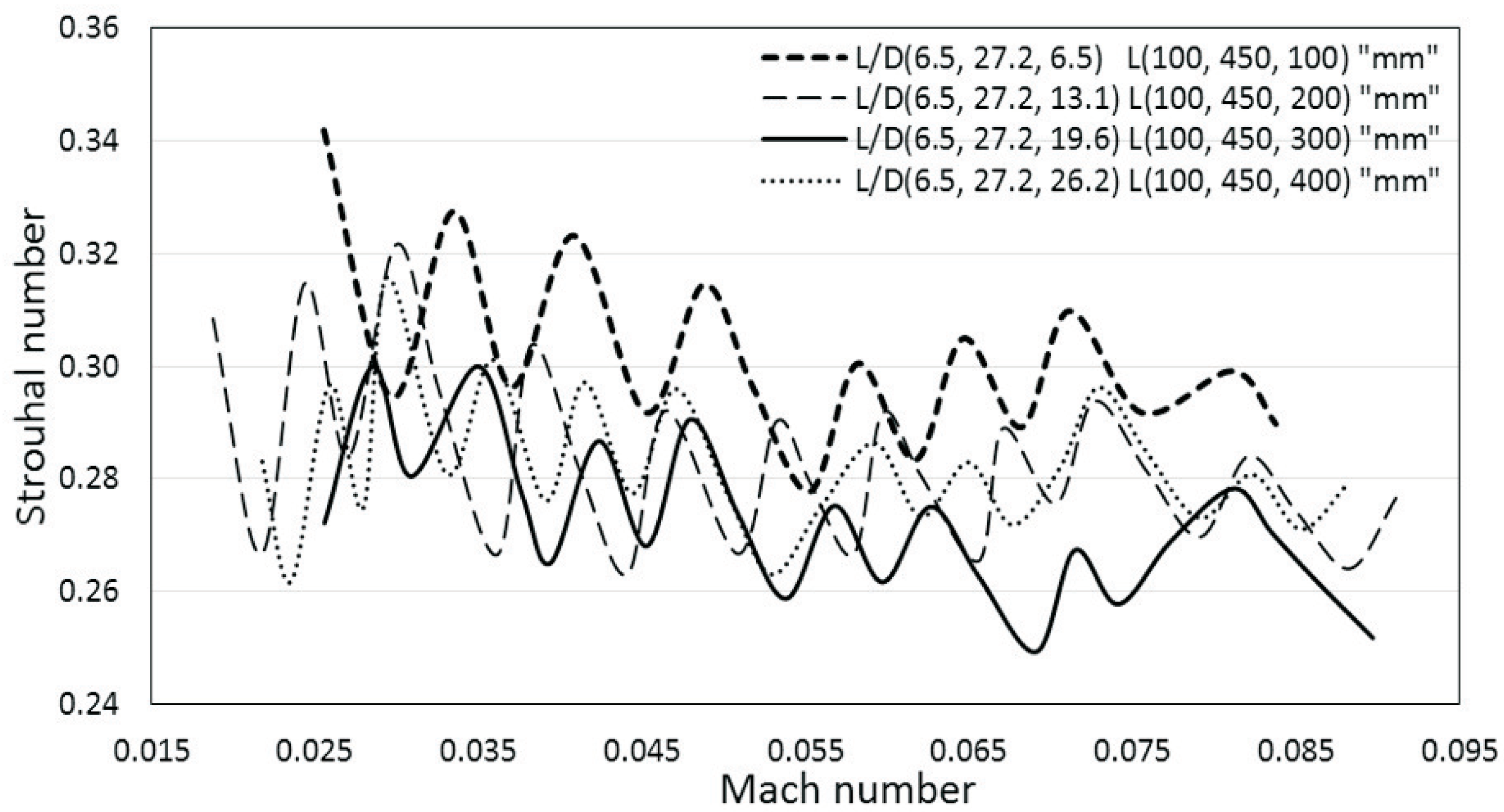
4.3. Longest Corrugated Segment: Case a-III ($L_{corr}/D_{corr}=$ 27.3)

Pipe systems in Case a-III, which have the longest corrugated pipe considered in this study, $L_{corr}=450$ mm, showed behavior similar to that in Cases a-I and a-II: increasing $L_{dw}$ while maintaining $L_{up}=100$ mm increased the frequency and Mach number ranges within which whistling occurred, as shown in Figure 11 and

Table 7. Mach number and corresponding frequency range (Hz) for pipe systems in Case a-III.

${\mathit{L}}_{\mathit{up}}$ (mm)	${\mathit{L}}_{\mathit{corr}}$ (mm)	${\mathit{L}}_{\mathit{dw}}$ (mm)	Mach Number Range	Corresponding Frequency Range (Hz)
100	450	100	0.026–0.084	1000–2700
		200	0.019–0.091	650–2800
		300	0.026–0.090	800–2550
		400	0.022–0.088	700–2750

. For $L_{up}=L_{dw}=100$ mm, the system whistled from M = 0.026 to 0.084 with whistling frequencies between 1000 and 2700 Hz. For $L_{dw}=200$ mm, the Mach number range was between M = 0.019 and 0.091, which correspond to frequencies of 650 and 2800 Hz, respectively. For $L_{dw}=300$ mm, the whistling range lay between M = 0.026 and 0.090, and the corresponding frequencies lay between 800 and 2,550 Hz. Finally, for the downstream pipe of length 400 mm, whistling frequencies were between 700 and 2750 Hz for Mach numbers of M = 0.022 and 0.088, respectively.

For $L_{dw}=100$ mm, the initial and final Strouhal numbers were 0.34 and 0.29 at M = 0.026 and 0.084, respectively, with a maximum Strouhal number of 0.34. For $L_{dw}=200$ mm, the initial and final Strouhal numbers were 0.31 and 0.28 with corresponding Mach numbers of 0.019 and 0.091, respectively. The maximum Strouhal number for this case was estimated to be 0.32.

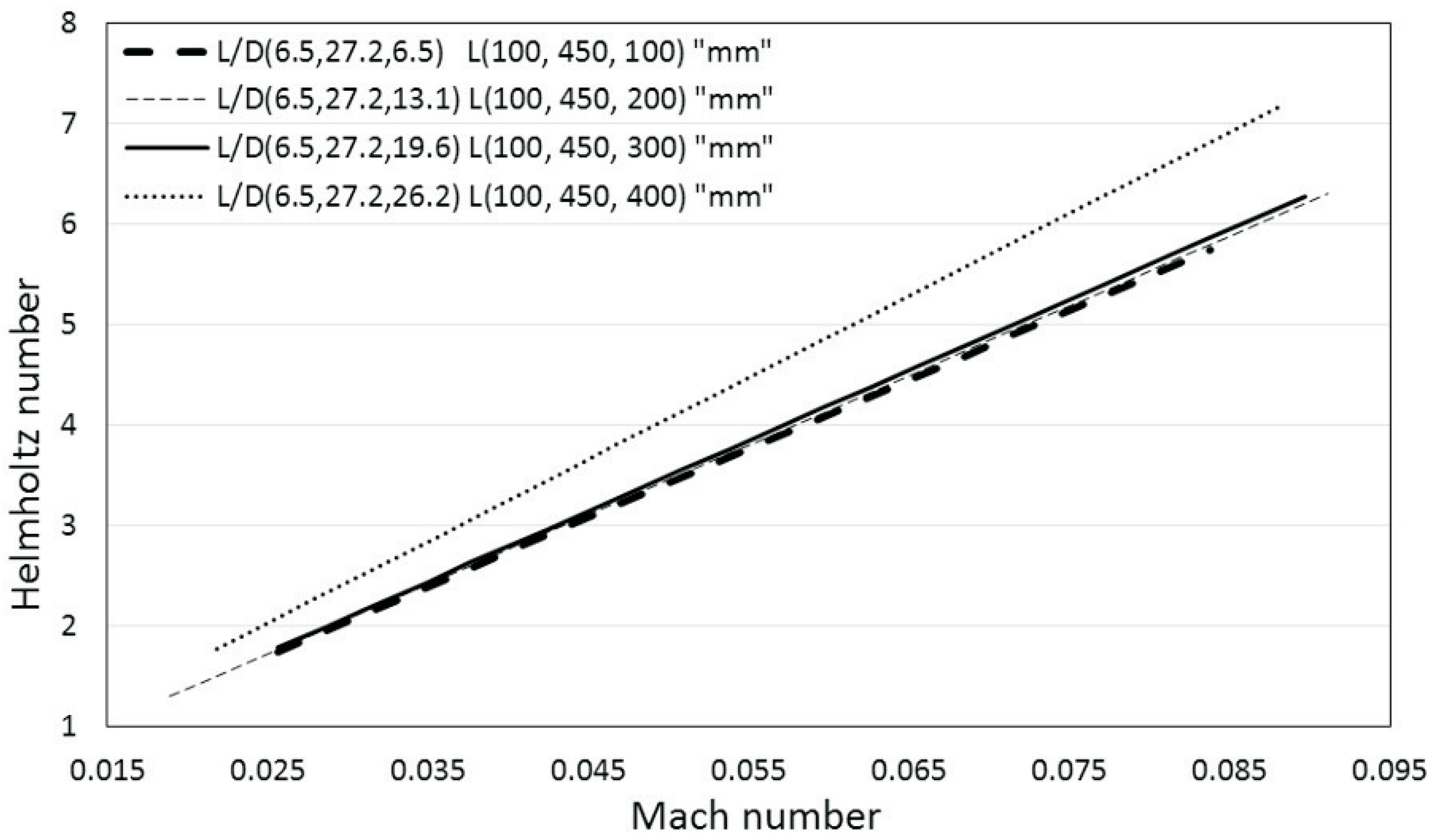
For $L_{dw}=300$ mm, the Strouhal numbers began and ended at 0.27 and 0.25, corresponding to M = 0.026 and 0.090, respectively, with a maximum $St$ of 0.30 occurring at multiple Mach numbers. Finally, for $L_{dw}=400$ mm, the initial and final Strouhal numbers had the same value of 0.28 at the minimum and maximum Mach numbers of 0.022 and 0.088, with a maximum $St$ of 0.32 in the whistling range, as shown in Figure 12 and

Table 8. Mach number range, corresponding Strouhal number ($St$) range and maximum Strouhal number for each pipe configuration in Case a-III.

${\mathit{L}}_{\mathit{up}}$ (mm)	${\mathit{L}}_{\mathit{corr}}$ (mm)	${\mathit{L}}_{\mathit{dw}}$ (mm)	Mach Number Range	Corresponding St Range	Max. St
100	450	100	0.026–0.084	0.34–0.29	0.34
		200	0.019–0.091	0.31–0.28	0.32
		300	0.026–0.090	0.27–0.25	0.30
		400	0.022–0.088	0.28–0.28	0.32

. Figure 13 and

Table 9. Mach number and corresponding Helmholtz number ($He$) range for pipe systems in Case a-III.

${\mathit{L}}_{\mathit{up}}$ (mm)	${\mathit{L}}_{\mathit{corr}}$ (mm)	${\mathit{L}}_{\mathit{dw}}$ (mm)	Mach Number Range	Corresponding He Range
100	450	100	0.026–0.084	1.75–5.74
		200	0.019–0.091	1.30–6.31
		300	0.026–0.090	1.79–6.28
		400	0.022–0.088	1.77–7.18

shows that for $L_{dw}=100$ mm, the range of $He$ was 1.75 to 5.74, which correspond to M = 0.026 and 0.084, respectively. For $L_{dw}=200$ mm, the minimum and maximum $He$ were estimated to be 1.30 and 6.31 at M = 0.019 and 0.091, respectively. The minimum and maximum $He$ for the downstream length of $L_{dw}=300$ mm were 1.79 and 6.28 at M = 0.026 and 0.090, respectively.

For the longest downstream smooth pipe of length 400 mm, the minimum $He$ at M = 0.022 was 1.77, whereas the maximum $He$ at M = 0.088 was 7.18. Figure 13 demonstrates that increasing the length of the downstream smooth segment augments the range of Helmholtz numbers for a constant corrugated pipe length.

5. Effect of Upstream Smooth Pipe Length on the Whistling Behavior for Constant Corrugated Segment Length (Case b)

5.1. Shortest Corrugated Segment: Case b-I ($L_{corr}/D_{corr}=$ 15.2)

In this section, we discuss the results of the cases in which $L_{up}$ varied for the three corrugated segment lengths considered in this study while maintaining the downstream segment length at a fixed value of 100 mm. For $L_{corr}=250$ mm with $L_{up}=L_{dw}=100$ mm, the results were discussed in Section 4.1. For $L_{up}=200$ mm, the whistling range decreased substantially from the case of $L_{up}=L_{dw}=100$ mm, with narrow ranges of Mach numbers from M = 0.032 to 0.044 and frequencies from 1150 to 1450 Hz. For $L_{up}=300$ mm, the Mach numbers ranged from M = 0.026 to 0.041 with corresponding whistling frequencies between 1000 and 1500 Hz.

However, for $L_{up}=400$ mm, the Mach number range was found to broaden in comparison with $L_{up}=200$ and 300 mm, although it was still very small compared with that of $L_{up}=100$ mm. For this particular case, whistling occurred between M = 0.031 and 0.048 with frequencies ranging from 1100 to 1550 Hz. Again, in Figure 14 and

Table 10. Mach number and corresponding frequency range (Hz) for pipe systems in Case b-I.

${\mathit{L}}_{\mathit{up}}$ (mm)	${\mathit{L}}_{\mathit{corr}}$ (mm)	${\mathit{L}}_{\mathit{dw}}$ (mm)	Mach Number Range	Corresponding Frequency Range (Hz)
100	250	100	0.027–0.069	1100–2500
200			0.032–0.044	1150–1450
300			0.026–0.041	1000–1500
400			0.031–0.048	1100–1550

, it is clear that the overall whistling range does not cover very high frequencies or Mach numbers because the length of the corrugated pipe used in this study is quite small. Evidently, fewer corrugations result in low-frequency whistling and smaller Mach number range. Varying the upstream and downstream lengths has a limited effect on enhancing the whistling range. For $L_{up}=100$ mm, as mentioned in Case a-I, the initial and final Strouhal numbers were 0.36 and 0.32, corresponding to Mach numbers of M = 0.027 and 0.067, respectively, with a maximum Strouhal number of 0.36 in this range, as shown in Figure 15 and

Table 11. Mach number range, corresponding Strouhal number ($St$) range and maximum Strouhal number for each pipe configuration in Case b-I.

${\mathit{L}}_{\mathit{up}}$ (mm)	${\mathit{L}}_{\mathit{corr}}$ (mm)	${\mathit{L}}_{\mathit{dw}}$ (mm)	Mach Number Range	Corresponding St Range	Max. St
100	250	100	0.027–0.069	0.36–0.32	0.36
200			0.032–0.044	0.33–0.30	0.33
300			0.026–0.041	0.34–0.32	0.34
400			0.031–0.048	0.31–0.29	0.31

. For the upstream length of 200 mm, the Strouhal numbers were estimated to start and end at 0.33 and 0.30 for corresponding Mach numbers of M = 0.032 and 0.044, respectively, with a maximum $St$ of 0.33. With the upstream smooth pipe of length 300 mm, the Strouhal number at the minimum and maximum Mach numbers of M = 0.026 and 0.041 were 0.34 and 0.32, respectively. The maximum $St$ in the whistling range was 0.34. Finally, with the longest upstream smooth pipe with length $L_{up}=400$ mm, the initial and final Strouhal numbers were 0.31 and 0.29 at M = 0.031 and 0.048, respectively, with a maximum of $St$ = 0.31.

Figure 16 and

Table 12. Mach number and corresponding Helmholtz number ($He$) range for pipe systems in Case b-I.

${\mathit{L}}_{\mathit{up}}$ (mm)	${\mathit{L}}_{\mathit{corr}}$ (mm)	${\mathit{L}}_{\mathit{dw}}$ (mm)	Mach Number Range	Corresponding He Range
100	250	100	0.027–0.069	1.31–3.38
200			0.032–0.044	1.73–2.41
300			0.026–0.041	1.76–2.75
400			0.031–0.048	2.25–3.41

show that, for the smallest upstream pipe of 100 mm, the minimum Helmholtz number $He$ at M = 0.027 is 1.31, whereas the highest $He$ at M = 0.069 is 3.38. For $L_{up}=200$ mm, the minimum and maximum $He$ are 1.73 and 2.41 at M = 0.032 and 0.044, respectively. The minimum and maximum $He$ for $L_{up}=300$ mm are 1.76 and 2.75 at M = 0.026 and 0.041, respectively. For the longest upstream smooth pipe of length 400 mm, the minimum $He$ at M = 0.031 is 2.25, whereas the maximum $He$ at M = 0.048 is 3.41. This particular case showed fluctuating behavior. It decreased at first but then increased again from the third configuration and continued to increase.

5.2. Intermediate Corrugated Segment: Case b-II ($L_{corr}/D_{corr}=$ 21.2)

The next configuration to be discussed is the pipe system with a 350 mm corrugated pipe. This particular configuration showed an overall increasing trend regarding (the frequency and Mach number ranges) with increasing upstream pipe length, as shown in Figure 17 and

Table 13. Mach number and corresponding frequency range (Hz) for pipe systems in Case b-II.

${\mathit{L}}_{\mathit{up}}$ (mm)	${\mathit{L}}_{\mathit{corr}}$ (mm)	${\mathit{L}}_{\mathit{dw}}$ (mm)	Mach Number Range	Corresponding Frequency Range (Hz)
100	350	100	0.023–0.078	850–2600
200			0.023–0.081	750–2750
300			0.017–0.056	850–2600
400			0.026–0.081	950–2700

. For upstream and downstream pipes with equal lengths of 100 mm, the lowest and highest Mach numbers were M = 0.023 and 0.078 with whistling frequencies ranging from 850 to 2600 Hz. For $L_{up}=200$ mm, the minimum and maximum Mach numbers were M = 0.023 and 0.081 with frequencies of 750 and 2750 Hz, respectively. Surprisingly, for $L_{up}=300$ mm, we observed a significant reduction in the Mach number range, extending from M = 0.017 to 0.056, but the frequency range had increased. Even at the lower modes, the pipe system whistled at higher intensities with frequencies ranging from 850 to 2600 Hz. Finally, the 400 mm upstream pipe followed the initial trend of increased whistling range from M = 0.026 to 0.081 with frequencies from 950 to 2700 Hz.

When the upstream and downstream smooth pipe lengths had equal lengths of 100 mm for the corrugated length of 350 mm, the initial and final Strouhal numbers were 0.34 and 0.30 at M = 0.023 and 0.078, respectively, with a maximum $St$ of 0.35. For $L_{up}=200$ mm, the $St$ at the minimum and maximum Mach numbers of M = 0.023 and 0.081 were 0.30 with 0.32, respectively, as the highest achieved value of Strouhal number for this configuration. As the upstream length increased to 300 mm, we estimated the $St$ values to begin and end at 0.35 and 0.32 with corresponding Mach numbers of M = 0.017 and 0.056, respectively, and the maximum $St$ was 0.37.

With further augmentation of the upstream length to 400 mm, the starting and ending $St$ were 0.32 and 0.30 at M = 0.026 and 0.081, respectively, with a maximum $St$ of 0.34 in this range, as shown in Figure 18 and

Table 14. Mach number range, corresponding Strouhal number ($St$) range and maximum Strouhal number for each pipe configuration in Case b-II.

${\mathit{L}}_{\mathit{up}}$ (mm)	${\mathit{L}}_{\mathit{corr}}$ (mm)	${\mathit{L}}_{\mathit{dw}}$ (mm)	Mach Number Range	Corresponding St Range	Max. St
100	350	100	0.023–0.078	0.34–0.30	0.35
200			0.023–0.081	0.30–0.30	0.32
300			0.017–0.056	0.35–0.32	0.37
400			0.026–0.081	0.32–0.30	0.34

.

As shown in Figure 19 and

Table 15. Mach number and corresponding Helmholtz number ($He$) range for pipe systems in Case b-II.

${\mathit{L}}_{\mathit{up}}$ (mm)	${\mathit{L}}_{\mathit{corr}}$ (mm)	${\mathit{L}}_{\mathit{dw}}$ (mm)	Mach Number Range	Corresponding He Range
100	350	100	0.023–0.078	1.29–4.36
200			0.023–0.081	1.31–4.71
300			0.017–0.056	1.36–4.54
400			0.026–0.081	2.22–6.79

, for the smallest upstream pipe of length 100 mm, the minimum Helmholtz number $He$ was 1.29 at M = 0.023, whereas the maximum $He$ was 4.36 at M = 0.078. For $L_{up}=200$ mm, the minimum and maximum $He$ were 1.31 and 4.71 at M = 0.023 and 0.081, respectively. The minimum and maximum $He$ for $L_{up}=300$ mm were 1.36 and 4.54 at M = 0.017 and 0.056, respectively. For the longest upstream smooth pipe of length 400 mm, the minimum $He$ was 2.22 at M = 0.026, whereas the maximum $He$ was 6.79 at M = 0.081. This particular trend suggests that the range of $He$ with respect to M continuously increases as the length of upstream smooth pipe increases, except in the case of the 300 mm upstream pipe, which resulted in the reduction of $He$ but started to whistle at a lower Mach number than all other configurations.

5.3. Longest Corrugated Segment: Case b-III ($L_{corr}/D_{corr}=$ 27.3)

Pipe systems in Case b-III, which have the longest corrugated pipe considered in this study, $L_{corr}=450$ mm, showed behavior similar to Cases b-I and b-II; increasing $L_{up}$ while maintaining $L_{dw}$ at 100 mm increased the range of whistling frequency and Mach number, as shown in Figure 20 and

Table 16. Mach number and corresponding frequency range (Hz) for pipe systems in Case b-III.

${\mathit{L}}_{\mathit{up}}$ (mm)	${\mathit{L}}_{\mathit{corr}}$ (mm)	${\mathit{L}}_{\mathit{dw}}$ (mm)	Mach Number Range	Corresponding Frequency Range (Hz)
100	450	100	0.026–0.084	1000–2700
200			0.024–0.086	850–2800
300			0.021–0.085	750–3100
400			0.022–0.093	700–2750

. For $L_{up}=L_{dw}=100$ mm, the system whistled from M = 0.026 to 0.084 with whistling frequencies between 1000 and 2700 Hz. For $L_{up}=200$ mm, the Mach number range was between M = 0.024 and 0.086, corresponding to frequencies of 850 and 2800 Hz, respectively. For $L_{up}=300$ mm, the whistling range lay between M = 0.021 to 0.085, with a corresponding range of frequencies between 750 and 3100 Hz. Finally, for the upstream pipe of length 400 mm, whistling frequencies ranged from 700 to 2750 Hz at M = 0.022 and 0.093, respectively.

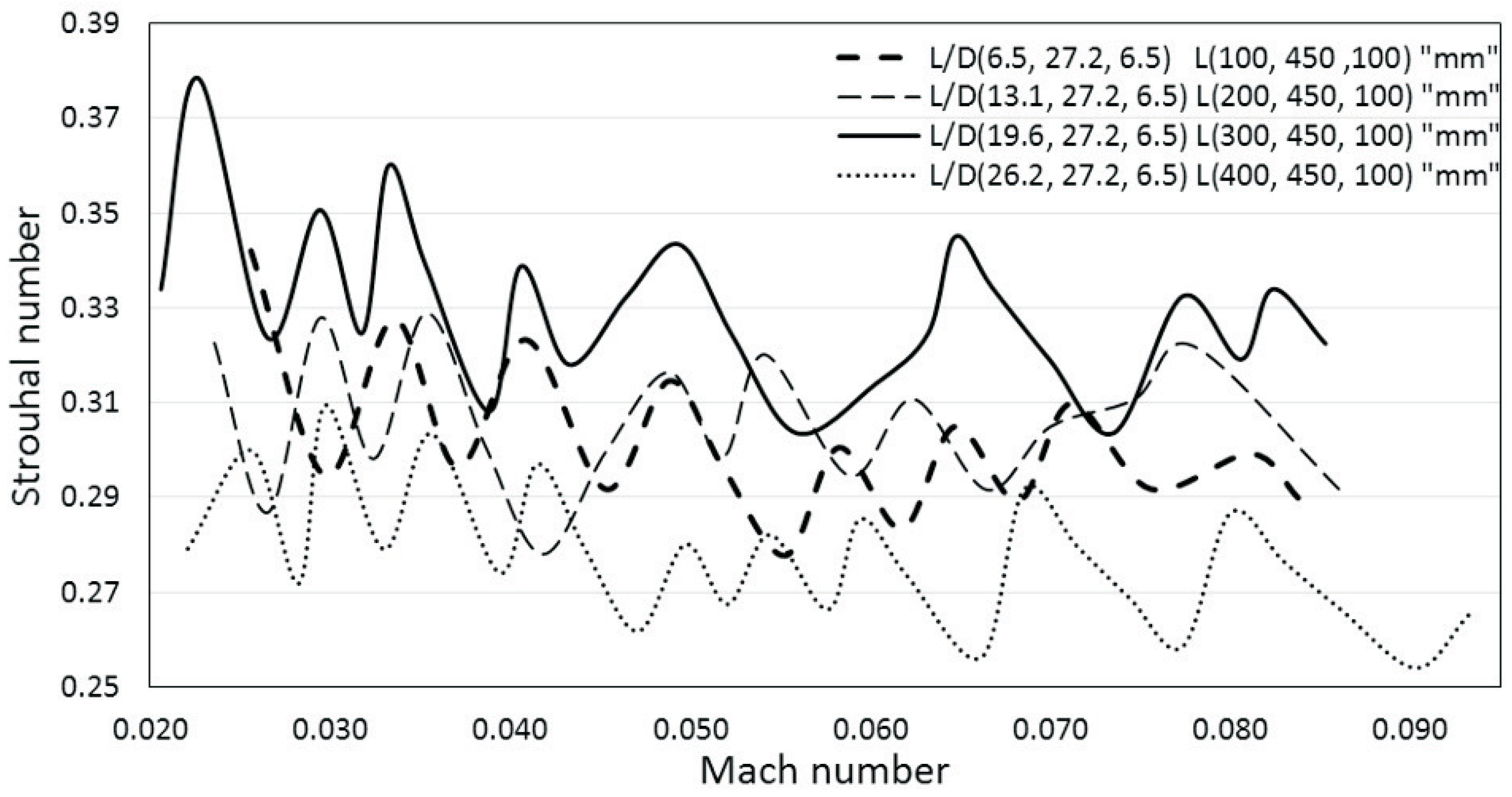
For $L_{up}=100$ mm, the initial and final Strouhal numbers were 0.34 and 0.29 at M = 0.026 and 0.084, respectively, as shown in Figure 21 and

Table 17. Mach number range, corresponding Strouhal number ($St$) range and maximum Strouhal number for each pipe configuration in Case b-III.

${\mathit{L}}_{\mathit{up}}$ (mm)	${\mathit{L}}_{\mathit{corr}}$ (mm)	${\mathit{L}}_{\mathit{dw}}$ (mm)	Mach Number Range	Corresponding St Range	Max. St
100	450	100	0.026–0.084	0.34–0.29	0.34
200			0.024–0.086	0.32–0.29	0.33
300			0.021–0.085	0.33–0.32	0.38
400			0.022–0.093	0.28–0.27	0.31

, with a maximum of 0.34 in this range. For $L_{up}=200$ mm, the Strouhal numbers were 0.32 and 0.29 at the initial and final Mach numbers of M = 0.024 and 0.086, respectively, with a maximum of 0.33 in this range.

For the 300 mm upstream smooth pipe, the starting Strouhal number at Mach number M = 0.021 was 0.33 and the ending one was 0.32 at M = 0.085, with a maximum Strouhal number of 0.38 in this range; this was also the peak value of $St$ for all cases considered in this study. For $L_{up}=400$ mm, Strouhal numbers of 0.28 and 0.27 corresponded to the starting and ending Mach numbers of 0.022 and 0.093, respectively, with a maximum Strouhal number of 0.31 in this range.

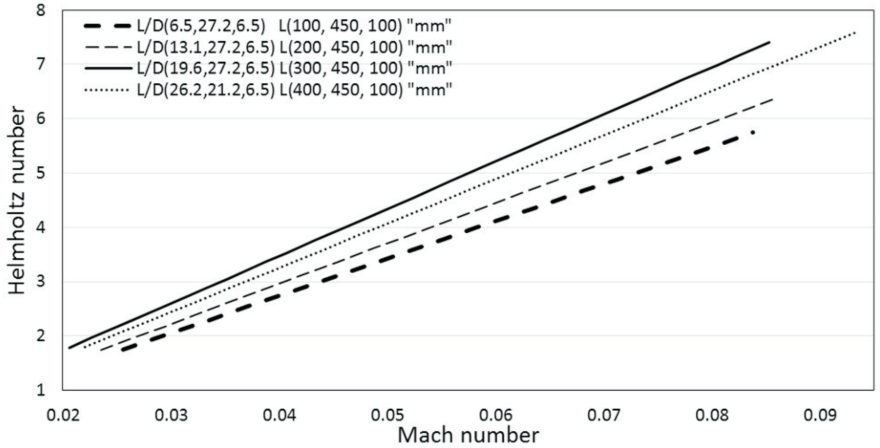
As shown in Figure 22 and

Table 18. Mach number and corresponding Helmholtz number ($He$) range for pipe systems in Case b-III.

${\mathit{L}}_{\mathit{up}}$ (mm)	${\mathit{L}}_{\mathit{corr}}$ (mm)	${\mathit{L}}_{\mathit{dw}}$ (mm)	Mach Number Range	Corresponding He Range
100	450	100	0.026–0.084	1.75–5.74
200			0.024–0.086	1.74–6.39
300			0.021–0.085	1.79–7.40
400			0.022–0.093	1.79–7.59

, for the smallest upstream pipe of length 100 mm, the minimum Helmholtz number $He$ was 1.75 at M = 0.026, whereas the maximum $He$ was 5.74 at M = 0.084. For $L_{up}=200$ mm, the minimum and maximum $He$ were 1.74 and 6.39 at M = 0.024 and 0.086, respectively. The minimum and maximum $He$ for $L_{up}=300$ mm were 1.79 and 7.40 at M = 0.021 and 0.085, respectively. For the longest upstream smooth pipe of length 400 mm, the minimum $He$ was 1.79 at M = 0.022, whereas the maximum $He$ was 7.59 at M = 0.093.

6. Acoustic Modes and Average Mode Gap

In this section, the whistling behaviors of various pipe configurations included in Cases a and b are discussed in terms of the acoustic modes and average mode gaps between successive modes. As shown in

Table 19. Excited acoustic mode numbers, mode numbers within the whistling range at which there was no whistling, and average mode gap between two successive modes for all configurations included in Case a. In the table, MN and MG denote Acoustic Mode Numbers and Mode Gap (Hz), respectively.

Pipe Configurations		${\mathit{L}}_{\mathit{up}}$ (mm)	${\mathit{L}}_{\mathit{corr}}$ (mm)	${\mathit{L}}_{\mathit{dw}}$ (mm)	Excited AMN	Missing MN	Average MG
Case a	I	100	250	100	3–7	-	350
				200	3–4	-	290
				300	-	-	-
				400	-	-	-
Case a	II	100	350	100	3–9	-	275
				200	3–9	8	245
				300	4–7	6	220
				400	4–8	-	190
Case a	III	100	450	100	4–11	-	245
				200	3–13	-	220
				300	4–13	-	195
				400	4–16	-	175

and

Table 20. Excited acoustic mode numbers, mode numbers within the whistling range at which there was no whistling, and average mode gap between two successive modes for all configurations included in Case b.

Pipe Configurations		${\mathit{L}}_{\mathit{up}}$ (mm)	${\mathit{L}}_{\mathit{corr}}$ (mm)	${\mathit{L}}_{\mathit{dw}}$ (mm)	Excited AMN	Missing MN	Average MG [Hz]
Case b	I	100	250	100	3–7	-	350
		200			4 and 5	-	300
		300			4–6	-	250
		400			5–7	-	220
Case b	II	100	350	100	3–9	-	275
		200			3–11	10	250
		300			3–11	9	215
		400			5–14	11 and 13	190
Case b	III	100	450	100	4–11	-	245
		200			4–13	-	220
		300			3–15	13	195
		400			4–16	12 and 14	170

, for each individual pipe system, there was significant variation in the excited acoustic mode numbers and the average mode gap between consecutive modes. For all configurations in Case a-I (see Table 19), increasing the length of the downstream smooth pipe resulted in a reduction in the number of excited acoustic modes from four modes (Modes 3–7) for $L_{dw}=100$ mm to a single excited acoustic mode for $L_{dw}=300$ and 400 mm. We could not predict which mode was excited in the last two pipe systems ($L_{dw}$ = 300 and 400 mm) corresponding to Case a-I, because at least two whistling frequencies are required to estimate the excited mode numbers and average mode gap. Moreover, the average mode gap also decreased with increasing $L_{dw}$. For configurations in Case a-II, a similar but less abrupt decrement in the number of excited modes occurred. The whistling covered Modes 3–9 for $L_{dw}=100$ mm, whereas for $L_{dw}=400$ mm, the whistling was found to occur between Modes 4 and 8. For configurations in this case with $L_{dw}=200$ and 300 mm, the pipe system did not whistle at Modes 8 and 6, respectively. The average mode gap decreased from 275 to 190 Hz for $L_{dw}$ = 100 and 400 mm, respectively. For Case a-III, the behavior was very much in contrast to the previous cases. The number of excited acoustic modes increased for increasing downstream smooth segment length. For $L_{dw}$ = 100 mm, the whistling range included Modes 4–11, whereas for $L_{dw}$ = 400 mm, this range consisted of Modes 4–16 with all modes included in the whistling range. The average mode gap showed a similar response to prior cases. For $L_{dw}$ = 100 mm, the average mode gap was 245 Hz, whereas for the longest downstream smooth pipe, $L_{dw}=400$ mm, the value was estimated to be 175 Hz.

The pipe systems in Case b have consistently increasing upstream smooth pipes with lengths ranging 100–400 mm with downstream pipe lengths fixed at 100 mm. For all configurations in Case b-I, increasing the length of the upstream smooth pipe results in a reduction in the number of excited acoustic modes. This behavior is very similar to that in Case a-I. For $L_{up}=100$ mm, the whistling covers acoustic Modes 3–7, whereas for $L_{up}=400$ mm, the whistling range included Modes 5–7. The average mode gap between successive modes for $L_{up}=100$ mm was 350 Hz, whereas for $L_{up}=400$ mm, it was estimated to be 220 Hz. For Case b-II, the number of excited acoustic modes increased continuously with increasing upstream lengths. It increased from seven modes (Modes 3–9) for $L_{up}=100$ mm to nine modes (Modes 5–14) for $L_{up}=400$ mm. For Case b-II, we observed that in all remaining configurations, with the exception of the configuration with an upstream segment of length 100 mm, whistling did not occur at some modes within the covered mode ranges during the whistling regime. Configurations with $L_{up}=$ 200 and 300 mm did not result in whistling at Modes 10 and 9, respectively, whereas Modes 11 and 13 were excluded in the case where $L_{up}=400$ mm. The average mode gap decreased from 275 to 190 Hz with increasing $L_{up}$ from 100 to 400 mm, respectively. For Case b-III, the number of excited modes continued to increase with increasing upstream length. The shortest upstream length of 100 mm covered Modes 4–11, whereas for the longest upstream length of 400 mm, the range was broadened to include modes 4 to 16. Mode 13 was excluded for the pipe system with $L_{up}=300$ mm, whereas Modes 12 and 14 were excluded for the configuration with $L_{up}=400$ mm. The average mode gap began at 245 Hz and decreased to 170 Hz when increasing the upstream length from $L_{up}$ = 100 to 400 mm. In both Cases a and b, the range of frequencies corresponding to the average mode gap showed a continuous downhill trend as the corrugated pipe length increased. The reason for the excluded modes reported for some configurations in both cases in not yet known.

7. Conclusions

This paper presents the results obtained from an experimental study in which both ends of a corrugated pipe were attached to smooth pipes. Three different corrugated pipe lengths (250, 350, and 450 mm) and four different smooth pipe lengths (100, 200, 300, and 400 mm) were included in the scope of our study. The configurations were divided into two cases, each of which was divided into three sub-cases. Case a included pipe systems where $L_{dw}\ge L_{up}$, whereas Case b included configurations where $L_{dw}\le L_{up}$. Each corrugated pipe length was tested with each smooth pipe length, as was previously mentioned.

• Case a: For the 250 mm corrugated pipe, the whistling range decreased sharply as the downstream pipe length increased. The corrugated pipe of length 350 mm also showed a decreasing trend in its whistling range. For the 450 mm pipe, the behavior was completely different; the whistling remained in almost the same range of Mach numbers for all sub-cases.
• Case b: For the 250 mm corrugated pipe, the whistling range was again found to decrease with increasing smooth pipe length but not as abruptly as in Case a. For the 350 mm corrugated pipe, the Mach number range for the whistling consistently increased and reached a maximum for the longest smooth pipe. The number of excited acoustic modes also increased with increasing smooth pipe length. Finally, for $L_{corr}=450$ mm, the pipe system behaved in a manner similar to the corrugated pipe with the same length in Case a (Case a-III). The overall Mach number range showed very little variation, and, for longer smooth pipes, the range showed a slight increment.

The average mode gap between successive modes continuously decreased for both cases as the smooth pipe increased in length. As the corrugation length increased, a greater number of modes were excited. The corrugated pipe with a length of 450 mm was not significantly affected by increasing the upstream or downstream smooth pipes. This may be because the lengths of the smooth pipe were small considering the number of cavities in the corrugated segment. Smaller corrugated pipes showed less whistling as a result of the lower number of corrugations, because each cavity acts as a source of sound, as reported in the literature. To more clearly observe the effect of the lengths of the upstream and downstream smooth pipes on longer corrugated segments, even longer smooth pipes should be investigated.

References

- Belfroid, S.P.; Shatto, D.P.; Peters, R.M.C.A.M. Flow induced pulsations caused by corrugated tubes. In Proceedings of the ASME Conference Proceedings, Seattle, DC, USA, 11–15 November 2007. [Google Scholar]
- Goyder, H. Noise generation and propagation within corrugated pipes. J. Press. Vessel Technol. 2013, 135, 1–7. [Google Scholar] [CrossRef]
- Crawford, F.S. Singing corrugated pipes. Am. J. Phys. 1974, 42, 278–288. [Google Scholar] [CrossRef]
- Silverman, M.P.; Cushman, G.M. Voice of the dragon: The rotating corrugated resonator. Eur. J. Phys. 1989, 10, 298–304. [Google Scholar] [CrossRef]
- Serafin, S.; Kojs, J. Computer models and compositional applications of plastic corrugated tubes. Organ. Sound 2005, 10, 67–73. [Google Scholar] [CrossRef]
- Burstyn, W. Eine neue Pfeife (a new pipe). Z. Tech. Phys. 1922, 3, 179–180. [Google Scholar]
- Cermak, P. Uber die Tonbildung bei Metallschlauchen mit eingedracktem Spiral gang (On the sound generation in flexible metal hoses with spiraling grooves). Z. Tech. Phys. 1922, 23, 394–397. [Google Scholar]
- Gutin, L. On the sound field of a rotating propeller. Z. Tech. Phys. 1936, 12, 76–83. [Google Scholar]
- Nakamura, Y.; Fukamachi, N. Sound generation in corrugated tubes. Fluid Dyn. Res. 1991, 7, 255–261. [Google Scholar] [CrossRef]
- Petrie, A.M.; Huntley, I.D. The acoustic output produced by a steady airflow through a corrugated duct. J. Sound Vib. 1980, 70, 1–9. [Google Scholar] [CrossRef]
- Kristiansen, U.R.; Wiik, G.A. Experiments on sound generation in corrugated pipes with flow. J. Acoust. Soc. Am. 2007, 121, 1337–1344. [Google Scholar] [CrossRef] [PubMed]
- Kopev, V.F.; Mironov, M.A.; Solntseva, V.S. Aeroacoustic interaction in a corrugated duct. Acoust. Phys. 2008, 54, 197–203. [Google Scholar] [CrossRef]
- Rockwell, D. Oscillations of impinging shear layers. AIAA J. 1983, 21, 645–664. [Google Scholar] [CrossRef]
- Bruggeman, J.C.; Wijnands, P.J.; Gorter, J. Self-sustained low-frequency resonance in low-Mach-number gas flow through pipelines with side branch cavities. In Proceedings of the 10th Aeroacoustics Conference, Seattle, DC, USA, 9–11 July 1986. [Google Scholar]
- Tonon, D.; Landry, B.; Belfroid, S.; Willems, J.; Hofman, G.; Hirschberg, A. Whistling of a pipe system with multiple side branches: Comparison with corrugated pipes. J. Sound Vib. 2010, 329, 1007–1024. [Google Scholar] [CrossRef]
- Binnie, A.M. Self-induced waves in a conduit with corrugated walls II. Experiments with air in corrugated and finned tubes. Proc. R. Soc. Lond. 1961, 262, 179–191. [Google Scholar] [CrossRef]
- Cadwell, L.H. Singing corrugated pipes revisited. Am. J. Phys. 1994, 62, 224–227. [Google Scholar] [CrossRef]
- Elliott, J. Corrugated pipe flow. In Lecture Notes on the Mathematics of Acoustics; Wright, M.C.M., Ed.; Imperial College Press: London, UK, 2004; pp. 207–222. [Google Scholar]
- Rudenko, O.; Nakiboglu, G.; Holten, A.; Hirschberg, A. On whistling of pipes with a corrugated segment: Experiment and theory. J. Sound Vib. 2013, 332, 7226–7242. [Google Scholar] [CrossRef]
- Ziada, S.; Buhlmann, E. Flow induced vibration in long corrugated pipes. In Proceedings of the 5th International Conference on Flow-Induced Vibrations, Brighton, UK, 20–22 May 1991. [Google Scholar]
- Debut, V.; Antunes, J.; Moreira, M. Experimental study of the flow-excited acoustical lock-in in a corrugated pipe. In Proceedings of the 14th International Conference on Sound and Vibration, Cairns, Australia, 9–12 July 2007. [Google Scholar]
- Debut, V.; Antunes, J.; Moreira, M. Flow-acoustic interaction in corrugated pipes: Time domain simulation of experimental phenomena. In Proceedings of the 9th International Conference on Flow-Induced Vibrations, Prague, Czech Republic, 30 June–3 July 2008. [Google Scholar]
- Kristiansen, U.R.; Mattei, P.O.; Pinhede, C.; Amielh, M. Experimental study of the influence of low frequency flow modulation on the whistling behavior of a corrugated pipe. J. Acoust. Soc. Am. 2011, 130, 1851–1855. [Google Scholar] [CrossRef] [PubMed]
- Nakiboglu, G.; Belfroid, S.P.; Tonon, D.; Willems, J.F.; Hirschberg, A. A parametric study on the whistling of multiple side branch system as a model for corrugated pipes. In Proceedings of the ASME Conference Proceedings, Liverpool, UK, 11–15 October 2009. [Google Scholar]
- Nakiboglu, G.; Belfroid, S.P.; Willems, J.; Hirschberg, A. Whistling behavior of periodic systems: Corrugated pipes and multiple side branch system. Int. J. Mech. Sci. 2010, 52, 1458–1470. [Google Scholar] [CrossRef]
- Nakiboglu, G.; Belfroid, S.P.; Golliard, J.; Hirschberg, A. On the whistling of corrugated pipes: Effect of pipe length and flow profile. J. Fluid Mech. 2011, 672, 78–108. [Google Scholar] [CrossRef]
- Nakiboglu, G.; Manders, H.B.; Hirschberg, A. Aeroacoustic power generated by a compact axisymmetric cavity: Prediction of self-sustained oscillation and influence of the depth. J. Fluid Mech. 2012, 703, 163–191. [Google Scholar] [CrossRef]
- Howe, M.S. Theory of Vortex Sound; Cambridge University Press: Cambridge, UK, 2003. [Google Scholar]
- Howe, M.S. The dissipation of sound at an edge. J. Sound Vib. 1980, 70, 407–411. [Google Scholar] [CrossRef]
- Howe, M.S. Contributions to the theory of aerodynamic sound, with application to excess jet noise and the theory of the flute. J. Fluid Mech. 1975, 71, 625–673. [Google Scholar] [CrossRef]
- Daugherty, R.; Franzini, J.; Finnemore, E. Fluid Mechanics with Engineering Applications, SI metric ed.; McGraw-Hill: New York, NY, USA, 1989. [Google Scholar]
Figure 1.
Whistling mechanism in corrugated pipes [8].
Figure 2.
Complete pipe system consisting of smooth pipe segments attached to a corrugated segment (not to scale).
Figure 3.
Corrugated pipe geometry (not to scale).
Figure 4.
3D sketch of experimental set-up and pipe system.
Figure 5.
Frequency (Hz) plotted against Mach number M for mm, mm, and = 100–400 mm.
Figure 6.
Strouhal number plotted against Mach number M for mm, mm, and = 100–400 mm.
Figure 7.
Helmholtz number plotted against Mach number M for mm, mm, and = 100–400 mm.
Figure 8.
Figure 9.
Figure 10.
Figure 11.
Figure 12.
Figure 13.
Figure 14.
Frequency (Hz) plotted against Mach number M for = 100–400 mm, mm, and mm.
Figure 15.
Strouhal number plotted against Mach number M for = 100–400 mm, mm, and mm.
Figure 16.
Helmholtz number plotted against Mach number M for = 100–400 mm, mm, and mm.
Figure 17.
Figure 18.
Figure 19.
Figure 20.
Figure 21.
Figure 22.