Photovoltaic Power Forecasting Based on EEMD and a Variable-Weight Combination Forecasting Model

1
School of Economics and Management, North China Electric Power University, Beijing 102206, China
2
Department of Economics and Management, North China Electric Power University, Baoding 071003, Hebei, China
*
Author to whom correspondence should be addressed.
Sustainability 2018, 10(8), 2627; https://doi.org/10.3390/su10082627
Submission received: 28 June 2018
/
Revised: 20 July 2018
/
Accepted: 22 July 2018
/
Published: 26 July 2018
(This article belongs to the Section Energy Sustainability)
Abstract
:It is widely considered that solar energy will be one of the most competitive energy sources in the future, and solar energy currently accounts for high percentages of power generation in developed countries. However, its power generation capacity is significantly affected by several factors; therefore, accurate prediction of solar power generation is necessary. This paper proposes a photovoltaic (PV) power generation forecasting method based on ensemble empirical mode decomposition (EEMD) and variable-weight combination forecasting. First, EEMD is applied to decompose PV power data into components that are then combined into three groups: low-frequency, intermediate-frequency, and high-frequency. These three groups of sequences are individually predicted by the variable-weight combination forecasting model and added to obtain the final forecasting result. In addition, the design of the weights for combination forecasting was studied during the forecasting process. The comparison in the case study indicates that in PV power generation forecasting, the prediction results obtained by the individual forecasting and summing of the sequences after the EEMD are better than those from direct prediction. In addition, when the single prediction model is converted to a variable-weight combination forecasting model, the prediction accuracy is further improved by using the optimal weights.
1. Introduction
Compared with other energy sources, solar energy has advantages of universality, cleanliness, extendibility, and sustainability, and it is one of the most ideal renewable energy sources. In solar energy applications, PV power generation is one of the most important forms [1]. Because PV power generation does not need to consume any resources and will not cause damage to the environment, it will be the best way for human beings to develop electric power business in the future. Whether it is from the perspective of protecting the Earth’s environment, or the sustainable development of the Earth’s resources, or in order to solve the problem of human beings’ growing demand for electricity, PV power generation is of great significance and has a profound impact on social development. With the advancement of science and technology in recent years, PV power generation has developed rapidly, and it accounts for an increasing proportion of power generation. The PV system can be applied to rural household power systems, large-scale PV power plants in remote areas, micro grids, and so on [2,3,4], and it plays an important role.
Although PV power generation has many advantages, there are also some problems in PV power generation systems, such as how to maximize power production [5], how to achieve relay coordination, and how to coordinate fault current limiters [6,7,8,9]. However, the most serious problem is that the power output of PV power generation is not stable, and it is greatly affected by the intensity of sunlight. PV panels do not generate electricity when there is no light at night. However, once the weather changes during the day, the impact on the power output is also great. When there is a cloud on a sunny day, the output power of the PV power generation will fluctuate greatly. Therefore, in order to utilize solar energy better and vigorously develop PV power generation, it is necessary to master the law of PV power generation and accurately forecast the output power of PV power generation. Accurate PV power forecasting [10,11,12,13] can not only provide a reliable basis for system planning and dispatching, but also plays a vital role in system optimization, effective use of energy, and safe and stable operation of the power grid.
The time series prediction method [14,15] was widely applied in the early stages of PV power generation forecasting, but its prediction accuracy is poor. The grey prediction method [16,17] has also been used for forecasting, but the results are not stable. New emerging machine learning algorithms, such as support vector machines (SVM) [18,19] and random forest [20,21,22], have better prediction accuracies. The neural network algorithm [23,24] has better prediction efficacy and can reflect changes in PV power generation under complex weather conditions due to its strong learning ability.
In recent years, numerous experts and scholars have applied decomposition-reconstruction prediction models to predict targets that are obvious and have related fluctuations, such as wind speed and PV power generation. Two commonly used methods are wavelet analysis [25,26,27,28] and empirical mode decomposition (EMD) [29,30,31]. Both methods can decompose the original waveform and are able to improve the prediction accuracy; however, both have drawbacks. Wavelet analysis has poor adaptability, and EMD has problems such as end-point and over-envelope effects. Ensemble empirical mode decomposition (EEMD) [32,33,34,35,36,37] was developed to improve EMD by weakening the impact of modal aliasing and has been applied in several fields of prediction research.
Since the last century, experts and scholars have conducted research into combination forecasting [38,39,40]. These studies have determined that the combination forecasting method has better prediction accuracy than a single method and can relieve cases in which a single method has large prediction errors at individual points. Combination models were usually used to predict variables with smaller data sizes at that time, and most of the methods that had been used were simple time series methods. Researchers then realized that the accuracy of a prediction result can be improved by giving different weights to different methods. Recently, several studies have assigned different weights to each time point of different methods (i.e., variable-weight combination forecasting) [41,42,43,44]; however, the determination of the weights is a major problem in these studies.
Based on previous studies, this paper presents a PV power generation forecasting method based on EEMD and a variable-weight combination forecasting model to improve PV prediction accuracy. First, the EEMD method is applied to decompose PV power generation data, and then multiple components are converted into three sequences: low-frequency, intermediate-frequency, and high-frequency. The variable-weight combination forecasting model is then applied to these three groups of sequences used to perform the prediction to obtain the final prediction results. A comparison between the case study indicates that the EEMD method can decompose the entire waveform into multiple small components, which is more conducive to forecasting and improves the prediction accuracy, and the variable-weight combination forecasting model provides a significant improvement in the prediction accuracy in comparison with the single method. The solution of the weights in predictions using the harmonic mean (HM) method gives the best results.
2. PV Power Prediction Modelling Theory
2.1. EEMD
EEMD is an improvement to EMD, which is a new noise-assisted data analysis method. Its core function is to incorporate Gaussian white noise into the signal for multiple EMD decompositions, and the outcomes of multiple decompositions are averaged to obtain the final decomposition result. Due to the influence of noise, the model can prevent scale mixing in the decomposition. Because of the zero homogeneity of Gaussian white noise, the noise cancels out after the averaging algorithm, which makes the resulting decomposition sequence more valid. Ultimately, the EEMD method provides a significant improvement in the decomposition effect of the EMD method by notably reducing modal aliasing.
Two important parameters in the EEMD algorithm are the amplitude of the white noise (i.e., the ratio of the added white noise to the standard deviation of the original signal amplitude) and the total number of repeated EMD decompositions. Currently, there is no formula for the selection of these two parameters. Based on various literature and the experimental data from this paper, the amplitude is set from 0.1 to 0.4, and the number of decompositions is set at 150.
2.2. Method of the Optimal Weight Determination
This paper uses two methods to determine the optimal weights and discusses which is more suitable for application to variable-weight combination forecasting.
The first method is the HM method. The optimal weight of each method at each time point is obtained by the calculation of each error with the HM formula:
where ei is the error of model i at each time point.
The second method is the quadratic programming (QP) method.
We set E to be the sum of the squared errors of the variable-weight combination forecasting model:
The optimal weights of the variable-weight combination forecasting model can be expressed by the following optimization problems:
where eit is the error of model i at time point t, kit is the weights of model i at time point t.
The optimal weight of each time point for each method can be obtained by solving the problem.
2.3. Variable Weight Prediction Modelling
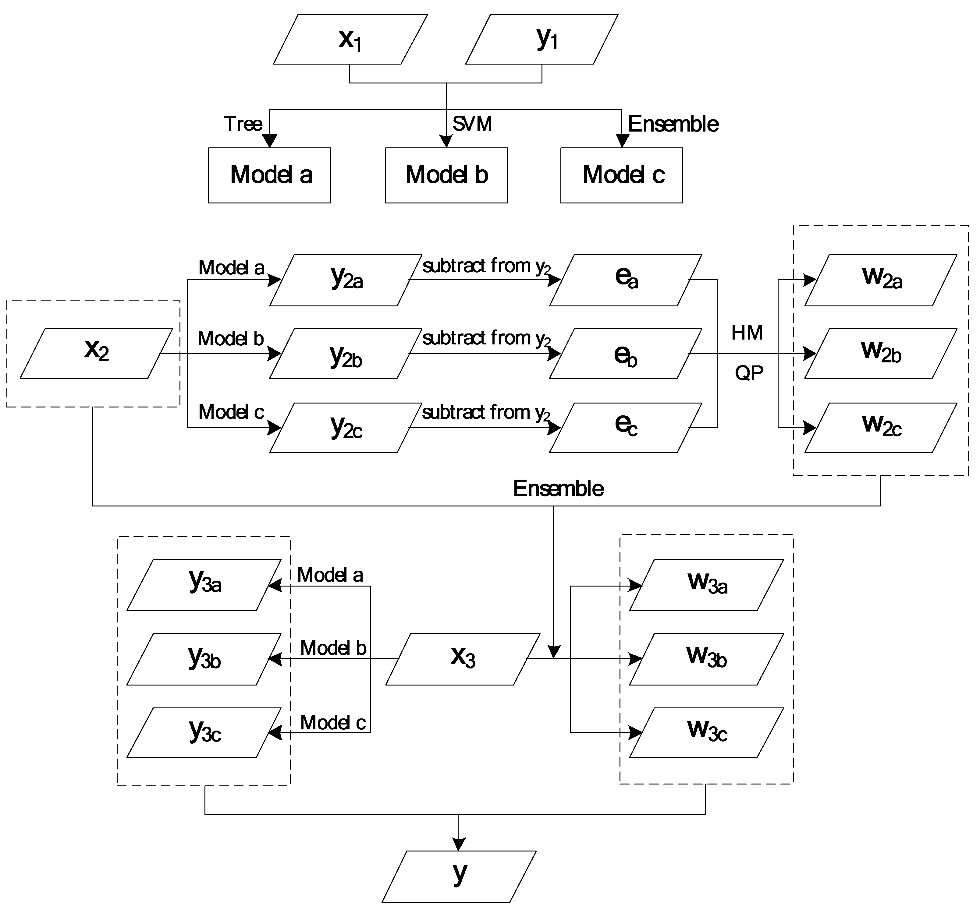
The original data used for the prediction are divided into three parts: a training set (x1, y1), an auxiliary set (x2, y2), and a test set (x3, y3). Models a, b, and c are obtained using the decision tree, SVM, and ensemble methods to conduct fitting of the training set. By using these models for the prediction of the auxiliary set x2, the prediction results, y2a, y2b, and y2c, of the auxiliary set are obtained. These are then subtracted from y2 to give the errors ea, eb, and ec, respectively. By using the HM or QP methods the optimal weights for the three prediction methods, w2a, w2b, and w2c, can be obtained. The ensemble method is then used to fit x2 with w2a, w2b, and w2c and predict the test set x3 to obtain the weights w3a, w3b, and w3c of each time point for each method. In addition, models a, b, and c are used to predict the test set x3 and obtain the prediction results y3a, y3b, and y3c. Finally, the variable weights of the three models are combined using the formula y = y3a × w3a + y3b × w3b + y3c × w3c, and the final prediction result is obtained. The design logic is shown in Figure 1.
3. PV Power Prediction Modelling Based on EEMD and the Variable-Weight Combination Forecasting Model
The prediction modelling procedure in this paper begins with the selection of the input variables. The lead time for the input variables is adjusted to one hour to make the prediction results practical. Modelling is then conducted using the EEMD and the variable-weight combination forecasting model, and the prediction results are output and evaluated.
3.1. Input Variable Selection
This paper presents the forecasting of hourly PV power generation. The lead time is 1 h, and there are 13 input variables: time, total column liquid water, total column ice water, surface pressure, relative humidity at 1000 mbar, total cloud cover, 10 m U wind component, 10 m V wind component, 2 m temperature [45], surface solar rad down, surface thermal rad down, top net solar rad, and total precipitation. Because time is a state variable, it is excluded from the SVM modelling.
3.2. Modelling Procedure
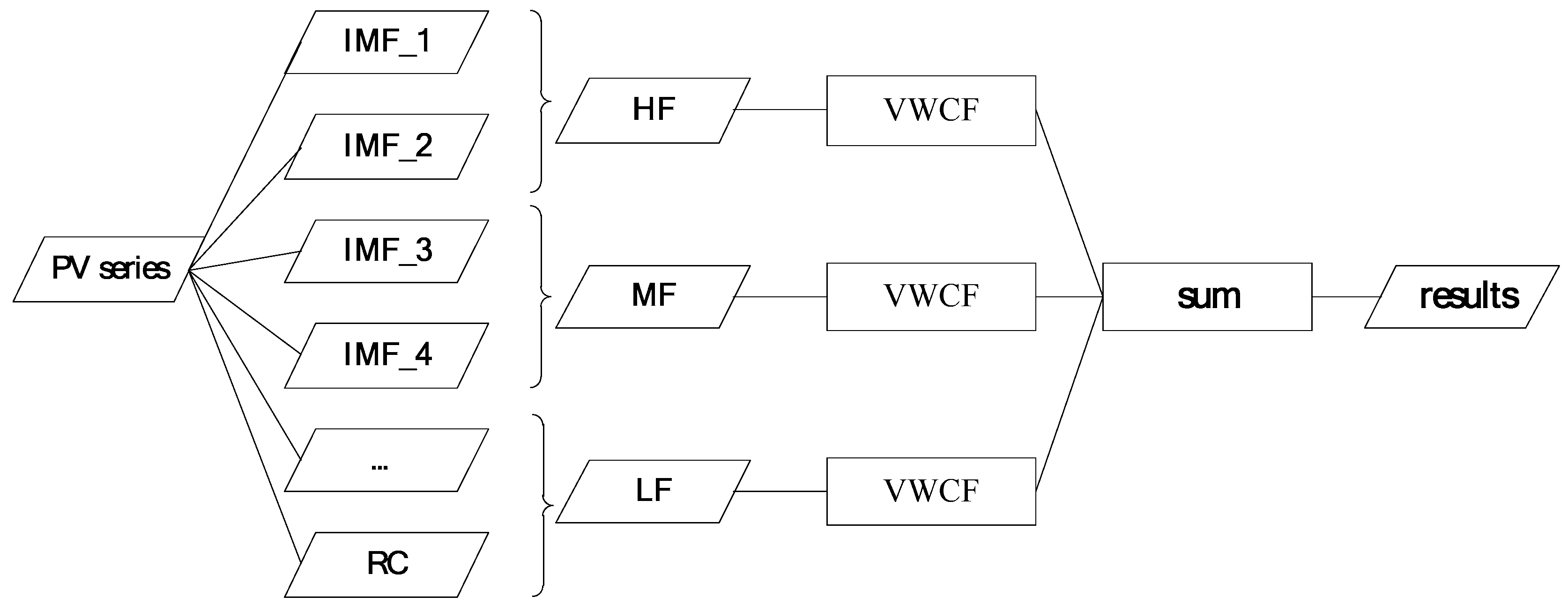
EEMD was used first to decompose the original PV power generation data to obtain multiple intrinsic mode function (IMF) components (IMF_1, IMF_2) and the residual component (RC). The IMF components and residual component were divided into high-frequency (HF), intermediate-frequency (MF), and low-frequency (LF) sequences based on several conditions. The variable-weight combination forecasting (VWCF) method was then applied to predict these three sequences. The sum of the three forecasting results gives the final prediction result. The flowchart of this process is shown in Figure 2.
3.3. Forecasting Results Evaluation
This paper uses the mean absolute error (MAE) and the mean square error (MSE) to evaluate the forecasting results obtained from the models. MAE and MSE are calculated using the following equations:
where is the predicted value, is the actual value, and is the sample size.
4. Empirical Analysis
4.1. Data Source and Parameter Initialization
This paper uses the PV power data from the CEFCom2014 competition, which were downloaded from the internet site http://www.gefcom.org. The time period was from 1 April 2012 to 29 June 2012. Because PV power is not generated at night, only the periods between 4 a.m. and 7 p.m. on these days are used as input data, and the periods between 5 a.m. to 8 p.m. are used as output data. A total of 1440 data points are used as the overall data set. The original data are divided into three groups of sequences: 960 for the training set, 320 for the auxiliary set, and 160 for the test set. Because the SVM method is used here, the original data must be normalized. This article uses MATLAB as a simulation tool.
4.2. EEMD and Variable Weight Combination Model
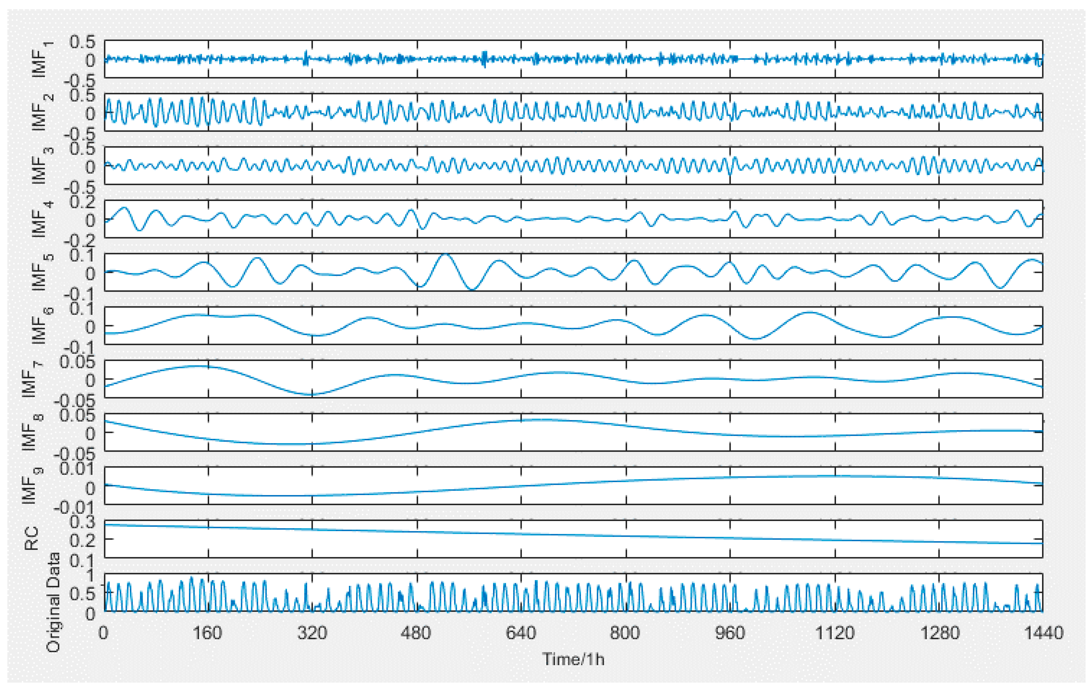
Figure 3 shows the decomposition results of the PV series using EEMD.
Ten sequence components are formed after the EEMD. The first three components are added to form the high-frequency sequence, components 4–6 are added to form the intermediate-frequency sequence, and the last four sequences are added to form the low-frequency sequence.
The “TREE + SVM + ENSEMBLE” combination prediction model is used to perform forecasting of the high-frequency, intermediate-frequency, and low-frequency sequences (the QP and HM methods are used for the weight selection), and the sum of the three forecasting results gives the final prediction result.
4.3. Comparison of the Models and Forecast Results
Based on the modelling, Figure 4 shows a comparison between the prediction results, and Table 1 shows a comparison of the forecasting evaluation indicators of each model.
Table 1 reveals that the use of the HM method for the variable-weight combination forecasting provides better results for the weight selection; the reason will be discussed in the next section. Compared to the model, the prediction results were worst when the decision tree method was used alone. When EEMD was used first and followed by the decision tree method, MAE decreased by 10.38% and MSE decreased by 42.7%. However, when using the proposed method (i.e., EEMD to decompose the data followed by a variable-weight combination forecasting model (HM)) compared with the EEMD + TREE, the MAE decreased by 8.79% and the MSE decreased by 6.14%, which further improves the PV power generation prediction accuracy.
The predictions using recent existing approaches and EEMD + VWCF (HM) are compared in Table 2.
In Table 2, we can see that EEMD + VWCF (HM) is better than recent existing single approaches like Random Forest and Back Propagation (BP) Neural Network both in MAE and MSE. When using EMD + VWCF (HM) compared with EMD + TREE, the MAE decreased by 4.06%, which shows that VWCF (HM) is a better method. Additionally, the comparison of EEMD + VWCF (HM) and EMD + VWCF (HM) shows that EEMD is an improvement to EMD.
Table 3 shows that the use of the QP method in the forecasting is significantly better than the use of the HM method when the weights of the three methods at each time point can be accurately predicted. However, because the weights obtained by the QP method are too extreme, the prediction model is not general. As a result, the final prediction accuracy of each sequence is essentially the same as that of the HM method. The final prediction results obtained after summing the three sequences show that the MAE and MSE of the QP method are worse than those of the HM method because its model is less general due to the extreme prediction, which leads to the low accuracy of the final prediction result.
4.4. Discussion on the Effects of Input Variables
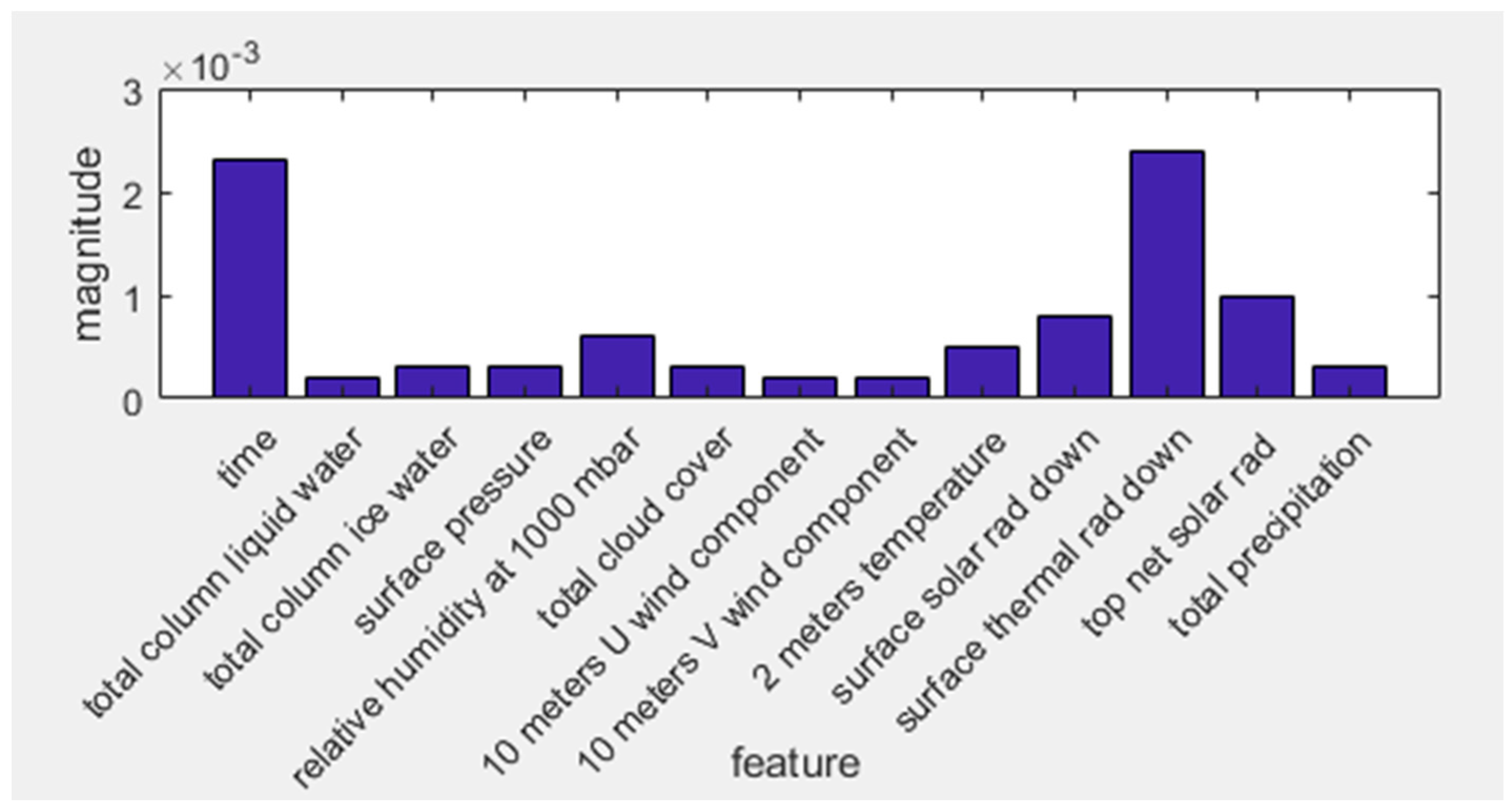
Since there are 13 input variables, and the influence of each variable on the prediction results is different, the degree of influence of each variable is discussed here. We can use the random forest algorithm to determine the impact of each variable as follows.
In Figure 5 we can see that the first six influential variables can be found and arranged in order: surface thermal rad down, time, top net solar rad, surface pressure, relative humidity at 1000 mbar, and 2 m temperature.
Table 4 shows that when only the six aforementioned variables are selected, in comparison to the results obtained from using all 13 variables, the prediction accuracy (in terms of MAE) of each model is reduced. The reason may be that although some variables have a small degree of influence, they can still affect the accuracy of the prediction in some cases. Therefore, each variable should be retained.
5. Conclusions
This paper proposed a PV power generation forecasting method based on EEMD and a variable-weight combination forecasting model. The sequences decomposed by EEMD are predicted using a variable-weight combination forecasting model individually and integrated to obtain the final forecasting result. The following conclusions are drawn from simulation experiments. After the waveform is decomposed by EEDM and reintegrated, the prediction accuracy of the PV power generation forecast model is significantly higher than that of the direct prediction; this reduces the impact of the non-stationary characteristics of the sequence on the prediction results. Variable-weight combination forecasting solves the problems that are present in single prediction methods, such as inaccurate predictions and large prediction errors at individual points. The HM method is most suitable for obtaining the weights of variable-weight combination forecasting models. The final prediction results show that the integration of EEMD with a variable-weight combination forecasting model can effectively improve the accuracy of PV power generation forecasting.
Author Contributions
In this research activity, all the authors were involved in the data collection and preprocessing phase, model construction, empirical research, results analysis and discussion, and manuscript preparation. All authors have approved the submitted manuscript.
Funding
The paper is supported by “the 111 Project (B18021)”.
Acknowledgments
We would like to thank the editor and reviewers for their constructive comments and helpful suggestions, which helped us to improve the manuscript.
Conflicts of Interest
The authors declare no conflict of interest.
References
- Singh, G.K. Solar power generation by PV (photovoltaic) technology: A review. Energy 2013, 53, 1–13. [Google Scholar] [CrossRef]
- Li, X.J.; Hui, D.; Lai, X.K. Battery energy storage station (BESS)-based smoothing control of photovoltaic (PV) and wind power generation fluctuations. IEEE Trans. Sustain. Energy 2013, 4, 464–473. [Google Scholar] [CrossRef]
- Nelson, D.B.; Nehrir, M.H.; Wang, C. Unit sizing and cost analysis of stand-alone hybrid wind/PV/fuel cell power generation systems. Renew. Energy 2006, 31, 1641–1656. [Google Scholar] [CrossRef]
- Kim, S.K.; Jeon, J.H.; Cho, C.H.; Kim, E.S.; Ahn, J.B. Modeling and simulation of a grid-connected PV generation system for electromagnetic transient analysis. Sol. Energy 2009, 83, 664–678. [Google Scholar] [CrossRef]
- Amirineni, S.S.T.; Morshed, M.J.; Fekih, A. Integral terminal sliding mode control for maximum power production in grid connected PV systems. In Proceedings of the 2016 IEEE Conference on Control Applications, Buenos Aires, Argentina, 19–22 September 2016. [Google Scholar]
- Ibrahim, D.K.; El Zahab, E.E.A.; Mostafa, S.A. New coordination approach to minimize the number of re-adjusted relays when adding DGs in interconnected power systems with a minimum value of fault current limiter. Int. J. Electr. Power Energy Syst. 2017, 85, 32–41. [Google Scholar] [CrossRef]
- Elmitwally, A.; Gouda, E.; Eladawy, S. Restoring recloser-fuse coordination by optimal fault current limiters planning in DG-integrated distribution systems. Int. J. Electr. Power Energy Syst. 2016, 77, 9–18. [Google Scholar] [CrossRef]
- Fani, B.; Hajimohammadi, F.; Moazzami, M.; Morshed, M.J. An adaptive current limiting strategy to prevent fuse-recloser miscoordination in PV-dominated distribution feeders. Electr. Power Syst. Res. 2018, 157, 177–186. [Google Scholar] [CrossRef]
- Jo, H.C.; Joo, S.K.; Lee, K. Optimal placement of superconducting fault current limiters (SFCLs) for protection of an electric power system with distributed generations (DGs). IEEE Trans. Appl. Supercond. 2013, 23, 5600304. [Google Scholar]
- Yang, H.T.; Huang, C.M.; Huang, Y.C.; Pai, Y.S. A weather-based hybrid method for 1-day ahead hourly forecasting of PV power output. IEEE Trans. Sustain. Energy 2014, 5, 917–926. [Google Scholar] [CrossRef]
- Raza, M.Q.; Nadarajah, M.; Ekanayake, C. On recent advances in PV output power forecast. Sol. Energy 2016, 136, 125–144. [Google Scholar] [CrossRef]
- Almeida, M.P.; Perpinan, O.; Narvarte, L. PV power forecast using a nonparametric PV model. Sol. Energy 2015, 115, 354–368. [Google Scholar] [CrossRef] [Green Version]
- Wu, Y.K.; Chen, C.R.; Rahman, H.A. A novel hybrid model for short-term forecasting in PV power generation. Int. J. Photoenergy 2014, 2014, 569249. [Google Scholar] [CrossRef]
- De Gooijer, J.G.; Hyndman, R.J. 25 years of time series forecasting. Int J. Forecast. 2006, 22, 443–473. [Google Scholar] [CrossRef] [Green Version]
- Khashei, M.; Bijari, M. A novel hybridization of artificial neural networks and ARIMA models for time series forecasting. Appl. Soft Comput. 2011, 11, 2664–2675. [Google Scholar] [CrossRef]
- Li, D.C.; Yeh, C.W.; Chen, C.C.; Wang, Y.T. A new grey prediction model for the return material authorization process in the TFT-LCD industry. Int. J. Adv. Manuf. Technol. 2018, 96, 2149–2160. [Google Scholar] [CrossRef]
- Kayacan, E.; Ulutas, B.; Kaynak, O. Grey system theory-based models in time series prediction. Expert Syst. Appl. 2010, 37, 1784–1789. [Google Scholar] [CrossRef]
- Quej, V.H.; Almorox, J.; Arnaldo, J.A.; Saito, L. ANFIS, SVM and ANN soft-computing techniques to estimate daily global solar radiation in a warm sub-humid environment. J. Atmos. Sol.-Terr. Phys. 2017, 155, 62–70. [Google Scholar] [CrossRef]
- Shamshirband, S.; Mohammadi, K.; Tong, C.W.; Zamani, M.; Motamedi, S.; Ch, S. A hybrid svm-ffa method for prediction of monthly mean global solar radiation. Theor. Appl. Climatol. 2016, 125, 53–65. [Google Scholar] [CrossRef]
- Ibrahim, I.A.; Khatib, T. A novel hybrid model for hourly global solar radiation prediction using random forests technique and firefly algorithm. Energy Convers. Manag. 2017, 138, 413–425. [Google Scholar] [CrossRef]
- Sun, H.W.; Gui, D.W.; Yan, B.W.; Liu, Y.; Liao, W.H.; Zhu, Y.; Lu, C.W.; Zhao, N. Assessing the potential of random forest method for estimating solar radiation using air pollution index. Energy Convers. Manag. 2016, 119, 121–129. [Google Scholar] [CrossRef] [Green Version]
- Ibarra-Berastegi, G.; Saenz, J.; Esnaola, G.; Ezcurra, A.; Ulazia, A. Short-term forecasting of the wave energy flux: Analogues, random forests, and physics-based models. Ocean Eng. 2015, 104, 530–539. [Google Scholar] [CrossRef]
- Senjyu, T.; Toyama, H.; Areekul, P.; Chakraborty, S.; Yona, A.; Urasaki, N.; Funabashi, T. Next-day peak electricity price forecasting using NN based on rough sets theory. IEEJ Trans. Electr. Electron. Eng. 2009, 4, 618–624. [Google Scholar] [CrossRef]
- Wang, F.; Mi, Z.Q.; Su, S.; Zhao, H.S. Short-term solar irradiance forecasting model based on artificial neural network using statistical feature parameters. Energies 2012, 5, 1355–1370. [Google Scholar] [CrossRef]
- Wang, D.; Borthwick, A.G.; He, H.D.; Wang, Y.K.; Zhu, J.Y.; Lu, Y.; Xu, P.C.; Zeng, X.K.; Wu, J.C.; Wang, L.C.; et al. A hybrid wavelet de-noising and rank-set pair analysis approach for forecasting hydro-meteorological time series. Environ. Res. 2018, 160, 269–281. [Google Scholar] [CrossRef] [PubMed]
- Liu, D.; Niu, D.X.; Wang, H.; Fan, L.L. Short-term wind speed forecasting using wavelet transform and support vector machines optimized by genetic algorithm. Renew. Energy 2014, 62, 592–597. [Google Scholar] [CrossRef]
- Emmanuel, M.; Rayudu, R.; Welch, I. Impacts of power factor control schemes in time series power flow analysis for centralized PV plants using wavelet variability model. IEEE Trans. Ind. Inform. 2017, 13, 3185–3194. [Google Scholar] [CrossRef]
- Liu, D.; Wang, J.L.; Wang, H. Short-term wind speed forecasting based on spectral clustering and optimised echo state networks. Renew. Energy 2015, 78, 599–608. [Google Scholar] [CrossRef]
- Li, F.F.; Wang, S.Y.; Wei, J.H. Long term rolling prediction model for solar radiation combining empirical mode decomposition (emd) and artificial neural network (ann) techniques. J. Renew. Sustain. Energy 2018, 10, 013704. [Google Scholar] [CrossRef]
- Guo, Z.H.; Zhao, W.G.; Lu, H.Y.; Wang, J.Z. Multi-step forecasting for wind speed using a modified emd-based artificial neural network model. Renew. Energy 2012, 37, 241–249. [Google Scholar] [CrossRef]
- He, K.J.; Zha, R.; Wu, J.; Lai, K.K. Multivariate emd-based modeling and forecasting of crude oil price. Sustainability 2016, 8, 387. [Google Scholar] [CrossRef]
- Wang, W.C.; Chau, K.W.; Xu, D.M.; Chen, X.Y. Improving forecasting accuracy of annual runoff time series using ARIMA based on EEMD decomposition. Water Resour. Manag. 2015, 29, 2655–2675. [Google Scholar] [CrossRef]
- Liu, Z.G.; Sun, W.L.; Zeng, J.J. A new short-term load forecasting method of power system based on EEMD and SS-PSO. Neural Comput. Appl. 2014, 24, 973–983. [Google Scholar] [CrossRef]
- Ouyang, Q.; Lu, W.X.; Xin, X.; Zhang, Y.; Cheng, W.G.; Yu, T. Monthly rainfall forecasting using EEMD-SVR based on phase-space reconstruction. Water Resour. Manag. 2016, 30, 2311–2325. [Google Scholar] [CrossRef]
- Li, T.Y.; Zhou, M.; Guo, C.Q.; Luo, M.; Wu, J.; Pan, F.; Tao, Q.Y.; He, T. Forecasting crude oil price using EEMD and RVM with adaptive pso-based kernels. Energies 2016, 9, 1014. [Google Scholar] [CrossRef]
- Yu, M.; Wang, B.; Zhang, L.L.; Chen, X. Wind speed forecasting based on EEMD and ARIMA. In Proceedings of the 2015 Chinese Automation Congress (CAC), Wuhan, China, 27–29 November 2015; pp. 1299–1302. [Google Scholar]
- Zhang, N.N.; Lin, A.J.; Shang, P.J. Multidimensional k-nearest neighbor model based on EEMD for financial time series forecasting. Phys. A Stat. Mech. Its Appl. 2017, 477, 161–173. [Google Scholar] [CrossRef]
- Li, H.M.; Wang, J.Z.; Lu, H.Y.; Guo, Z.H. Research and application of a combined model based on variable weight for short term wind speed forecasting. Renew. Energy 2018, 116, 669–684. [Google Scholar] [CrossRef]
- Song, J.J.; Wang, J.Z.; Lu, H.Y. A novel combined model based on advanced optimization algorithm for short-term wind speed forecasting. Appl. Energy 2018, 215, 643–658. [Google Scholar] [CrossRef]
- Zhang, F.Y.; Dong, Y.Q.; Zhang, K.Q. A novel combined model based on an artificial intelligence algorithm—A case study on wind speed forecasting in Penglai, China. Sustainability 2016, 8, 555. [Google Scholar] [CrossRef]
- Jiang, P.; Li, C. Research and application of an innovative combined model based on a modified optimization algorithm for wind speed forecasting. Measurement 2018, 124, 395–412. [Google Scholar] [CrossRef]
- Jiang, A.H.; Mei, C.; E, J.Q.; Shi, Z.M. Nonlinear combined forecasting model based on fuzzy adaptive variable weight and its application. J. Cent. South. Univ. Technol. 2010, 17, 863–867. [Google Scholar] [CrossRef]
- Li, L.H.; Mu, C.Y.; Ding, S.H.; Wang, Z.; Mo, R.Y.; Song, Y.F. A robust weighted combination forecasting method based on forecast model filtering and adaptive variable weight determination. Energies 2016, 9, 20. [Google Scholar] [CrossRef]
- Li, W.; Xie, H. Geometrical variable weights buffer gm(1,1) model and its application in forecasting of China’s energy consumption. J. Appl. Math. 2014, 2014, 131432. [Google Scholar] [CrossRef]
- Kaldellis, J.K.; Kapsali, M.; Kavadias, K.A. Temperature and wind speed impact on the efficiency of PV installations. Experience obtained from outdoor measurements in Greece. Renew. Energy 2014, 66, 612–624. [Google Scholar] [CrossRef]
Figure 1.
Flowchart of the variable-weight combination forecasting model.

Figure 2.
Flowchart of EEMD-VWCF model. PV: photovoltaic; RC: residual component; HF: high-frequency sequence; MF: intermediate-frequency component; LF: low-frequency component; VWCF: variable-weight combination forecasting; EEMD: ensemble empirical mode decomposition.
Figure 2.
Flowchart of EEMD-VWCF model. PV: photovoltaic; RC: residual component; HF: high-frequency sequence; MF: intermediate-frequency component; LF: low-frequency component; VWCF: variable-weight combination forecasting; EEMD: ensemble empirical mode decomposition.

Figure 3.
Decomposition results of the PV series using EEMD.

Figure 4.
Comparison of forecasting results of the models. QP: quadratic programming method; HM: harmonic mean method.
Figure 4.
Comparison of forecasting results of the models. QP: quadratic programming method; HM: harmonic mean method.

Figure 5.
Analysis of the effects of each input variable.


Table 1.
Comparison of the evaluation indicators of the models. MAE: mean absolute error; MSE: mean square error.
Table 1.
Comparison of the evaluation indicators of the models. MAE: mean absolute error; MSE: mean square error.
| Model | MAE | MSE |
|---|---|---|
| TREE | 0.0761 | 0.0199 |
| EEMD + TREE | 0.0682 | 0.0114 |
| EEMD + VWCF (QP) | 0.0697 | 0.0123 |
| EEMD + VWCF (HM) | 0.0622 | 0.0107 |
Table 2.
Comparison of recent existing approaches and EEMD + VWCF (HM).
| Model | MAE | MSE |
|---|---|---|
| Random Forest | 0.0833 | 0.0140 |
| Back Propagation (BP) Neural Network | 0.0816 | 0.0157 |
| EMD + TREE | 0.0713 | 0.0130 |
| EMD + VWCF (HM) | 0.0684 | 0.0127 |
| EEMD + VWCF (HM) | 0.0622 | 0.0107 |
Table 3.
Comparison of forecasting results of QP and HM methods.
| MAE of Different States | QP | HM |
|---|---|---|
| Optimal forecasting of LF | 0.0192 | 0.0267 |
| Last forecasting of LF | 0.0308 | 0.0313 |
| Optimal forecasting of MF | 0.0278 | 0.0381 |
| Last forecasting of MF | 0.0544 | 0.0556 |
| Optimal forecasting of HF | 0.0287 | 0.0460 |
| Last forecasting of HF | 0.0723 | 0.0717 |
| Last forecasting | 0.0697 | 0.0622 |
Table 4.
Comparison of results of the different methods using 6 and 13.
| MAE | 6 Variables | 13 Variables |
|---|---|---|
| TREE | 0.0761 | 0.0900 |
| EEMD + TREE | 0.0682 | 0.0826 |
| EEMD + VWCF (HM) | 0.0622 | 0.0773 |
© 2018 by the authors. Licensee MDPI, Basel, Switzerland. This article is an open access article distributed under the terms and conditions of the Creative Commons Attribution (CC BY) license (http://creativecommons.org/licenses/by/4.0/).
Share and Cite
MDPI and ACS Style
Wang, H.; Sun, J.; Wang, W. Photovoltaic Power Forecasting Based on EEMD and a Variable-Weight Combination Forecasting Model. Sustainability 2018, 10, 2627. https://doi.org/10.3390/su10082627
AMA Style
Wang H, Sun J, Wang W. Photovoltaic Power Forecasting Based on EEMD and a Variable-Weight Combination Forecasting Model. Sustainability. 2018; 10(8):2627. https://doi.org/10.3390/su10082627
Chicago/Turabian StyleWang, Hui, Jianbo Sun, and Weijun Wang. 2018. "Photovoltaic Power Forecasting Based on EEMD and a Variable-Weight Combination Forecasting Model" Sustainability 10, no. 8: 2627. https://doi.org/10.3390/su10082627
Note that from the first issue of 2016, this journal uses article numbers instead of page numbers. See further details here.