Detection of Frozen Soil Using Sentinel-1 SAR Data


1
IRSTEA, University of Montpellier, TETIS, F-34093 Montpellier CEDEX 5, France
2
CNRS, CESBIO, 31401 Toulouse CEDEX 9, France
*
Author to whom correspondence should be addressed.
Remote Sens. 2018, 10(8), 1182; https://doi.org/10.3390/rs10081182
Submission received: 18 June 2018
/
Revised: 19 July 2018
/
Accepted: 24 July 2018
/
Published: 26 July 2018
(This article belongs to the Section Remote Sensing in Agriculture and Vegetation)
Abstract
:The objective of this paper is to evaluate the potential of Sentinel-1 Synthetic Aperture Radar “SAR” data (C-band) for monitoring agricultural frozen soils. First, investigations were conducted from simulated radar signal data using a SAR backscattering model combined with a dielectric mixing model. Then, Sentinel-1 images acquired at a study site near Paris, France were analyzed using temperature data to investigate the potential of the new Sentinel-1 SAR sensor for frozen soil mapping. The results show that the SAR backscattering coefficient decreases when the soil temperature drops below 0 °C. This decrease in signal is the most important for temperatures that ranges between 0 and −5 °C. A difference of at least 2 dB is observed between unfrozen soils and frozen soils. This difference increases under freezing condition when the temperature at the image acquisition date decreases. In addition, results show that the potential of the C-band radar signal for the discrimination of frozen soils slightly decreases when the soil moisture decreases (simulated data were used with soil moisture contents of 20 and 30 vol%). The difference between the backscattering coefficient of unfrozen soil and the backscattering coefficient of frozen soil decreases by approximately 1 dB when the soil moisture decreases from 30 to 20 vol%). Finally, the results show that both VV and VH allow a good detection of frozen soils but the sensitivity of VH is higher by approximately 1.5 dB. In conclusion, this study shows that the difference between a reference image acquired without freezing and an image acquired under freezing conditions is a good tool for detecting frozen soils.
1. Introduction
Frost frequently causes serious crop damages and consequently loss of yield. A frozen soil map is a key tool to assess the extent of loss of yield in agricultural areas. This map requires a monitoring system that can map the frozen zones with fine spatial and temporal resolutions. The arrival of Sentinel-1 (S1) satellites encourages the analysis of Synthetic Aperture Radar (SAR) data for mapping agricultural frozen soils with a high revisit time and high spatial resolution (up to plot scale). Some studies have shown from SAR and radiometer-scatterometer data (e.g., ERS, ENVISAT/ASAR and RADARSAT) that the SAR backscattering coefficient decreases when soil freezes [1,2,3,4,5]. A decrease in the radar signal of approximately 3 dB was observed when the soil was frozen [2,3]. Wegmüller [1] studied the effect of freezing and thawing on the microwave signatures of bare soil using radiometer-scatterometer system at frequencies between 3 and 11 GHz. His results showed that freezing increases the emissivity and decreases the backscattering coefficient. Rignot et al. [2] observed from temporal ERS-1 SAR images (C-band) pronounced temporal variations in radar backscattering coefficient in Taiga forests due to freezing events. They detected a 3 dB decrease when the soil and vegetation freeze. Khaldoune et al. [3] mapped agricultural frozen soils under snow cover using RADARSAT-1 images (C-band). They developed classification algorithm based on soil-freezing threshold from the backscattering coefficient in HH polarization. Park et al. [4] used ENVISAT/ASAR images (C-band) to monitor freeze/thaw cycles of permafrost areas. A difference of 3–4 dB was observed between ASCAT signal in freezing condition and ASCAT signal in thawing condition. Jagdhuber et al. [5] showed over a study site in Finland the high sensitivity of RADARSAT-2 signal (C-band) to soil freezing and thawing states even under dry snow cover.
Under cold winter conditions, much of soil water freezes, which leads to a significant decrease of the soil dielectric constant. The decrease in the dielectric constant due to a decrease of the volumetric moisture content causes a decrease of the radar signal [6]. This variation in the radar signal due to the variation in the soil dielectric constant can be estimated using SAR images [1,2,3,4,5]. Currently, several high-resolution SAR images can be acquired at a given study site due to the availability of SAR data in the C-band (e.g., Radarsat-2 and Sentinel-1) and X-band (e.g., TerraSAR-X and COSMO-SkyMed). However, only Sentinel-1 satellites provide users with free and open access SAR data at high spatial and temporal resolutions (revisit time of six days over Europe and spatial resolution of 10 m). This high spatial resolution of SAR sensors will make it possible to follow the soil freezing at very fine spatial scales in agricultural areas (plot scale or sub-plot scale).
Recently, a freeze/thaw product generated from SMAP data is available at low spatial resolution [7]. The product based on temporal change detection approach assumes that the high variation in the temporal dynamics of the normalized polarization ratio (NPR) of the brightness temperature is related to a large change in dielectric constant (passing from frozen to non-frozen condition, or reciprocally) [7].
The objective of this paper is to study the potential of Sentinel-1 SAR data for monitoring agricultural frozen soils. A SAR backscattering model combined with a dielectric mixing model was used to study the behavior of the SAR signal after freezing. Assuming that the soil moisture and the surface roughness were unchanged between the date of unfrozen soil condition and the date of frozen soil condition, a time series of Sentinel-1 images acquired on a study site in France was analyzed to identify frozen soils. After a detailed description of the semi-empirical frozen soil–water dielectric mixing model is presented in Section 2, Section 3 describes the data used (modeling settings, Sentinel-1 images and temperature data). In Section 4, the results are given (dielectric constant behavior, SAR modeling on frozen soils, and interpretation of Sentinel-1 images). A discussion is presented in Section 5. Finally, Section 6 presents the main conclusions.
2. Radar Signal Modeling
To investigate the potential of the new C-band SAR Sentinel-1 sensor for monitoring frozen soils in an agricultural context, the radar backscattering coefficients of frozen soils were simulated using the Integral Equation model [8,9] and a dielectric constant model of frozen soil. In these simulations, only the case of bare soils was considered.
2.1. Semi-Empirical Dielectric Mixing Model for Frozen Soil–Water
Dobson et al. [10] developed a semi-empirical soil–water dielectric mixing model for the 1.4–18 GHz frequency range of the following form:
where is the relative complex dielectric constant of the soil–water mixture, is the real part and is the imaginary part. and are given by:
where is the bulk density (g/cm3), is the specific density of the solid soil particules (g/cm3), is the dielectric constant of soil solid, is the volumetric moisture content (vol%), is the real part of the dielectric constant of free water, is the imaginary part of the dielectric constant of free water, α is an empirically determined constant (=0.65 [10]), and and are soil-texture-dependent coefficients.
The dielectric constant of soil solid,, given in Equation (2), is expressed by Dobson et al. [10]:
For a given soil with = 2.66 g/cm3, = 4.7.
To calculate and of Equations (2) and (3), the following expressions are used [10,11]:
where S and C are the percentages of sand and clay, respectively.
The quantities and presented in Equations (2) and (3) are defined in Dobson et al. [10] and Peplinski et al. [11] as follows:
where = 4.9 is the high frequency limit of , is the static dielectric constant of water, f is the frequency (Hz), is the relaxation time for water, = 8.854 × 10⁻¹² F/m is the permittivity of free space, and is the effective conductivity.
In Equations (7) and (8), the expressions for the static dielectric constant of water, , and the relaxation time for water, , are given as a function of the water temperature () [12,13]:
For = 20 °C, = 80.1 and = 0.58 × 10⁻¹⁰ s.
The effective conductivity, , defined in Equation (8), is given by Peplinski et al. [11]:
An extension of this semi-empirical dielectric mixing model was proposed by Zhang et al. [14] to include freezing conditions. The dielectric constant of frozen soil–water mixture (= − j) is given by:
where is the unfrozen volumetric moisture content (vol%), is the volumetric ice content (vol%), and is the dielectric constant of ice (=3.15). and are given by Zhang et al. [14]:
where is the soil temperature steering the amount of liquid to frozen water in the soil (K), is the density of water (=1 g/cm3), is the specific density of ice (=0.9175 g/cm3) [5], and A and B are empirical coefficients related to soil texture. In Zhang et al. [14], A and B were calculated for three soil types (Silty-clay, Silt-loam and Sandy-loam, Table 1). For above 273.2 °K, = 0 and .
2.2. Radar Backscattering Model
In this study, the Integral Equation Model modified by Baghdadi (IEM_B) was used to simulate soil surface scattering in a context of bare agricultural fields. In addition to SAR instrumental parameters (radar wavelength, incidence angle and polarization), the radar signal depends on the soil dielectric constant and surface roughness (Hrms) [15,16,17,18,19]. Only the surface scattering was considered in this study, with one permittivity layer.
The IEM_B was used since it provides simulated SAR backscattering coefficients with a good accuracy (RMSE about 2 dB) [20]. In fact, several studies reported important discrepancies between backscattering coefficients simulated by the original IEM developed by Fung et al. [21] and those measured by SAR sensors [22,23,24]. According to Baghdadi et al. [25], this discrepancy is mainly due to the in situ measured correlation length “L” which is difficult to measure in the field with good accuracy. To reduce such discrepancies between simulated and measured backscattering values, Baghdadi et al. [8,9,26,27,28] proposed a semi-empirical calibration of the original IEM in order to improve the accuracy of the simulated backscattering values. This semi-empirical calibration consists of replacing the in situ measured correlation length by a fitting parameter, called Lopt. Lopt depends on surface roughness conditions and SAR configurations (incidence angle, polarization and radar wavelength). The calibrated IEM_B was carried separately at X-band in [27], C-band in [8,9] and L-band in [26]. The proposed calibration reduces the number of IEM’s input soil parameters from three to two parameters (root mean square surface height “Hrms” and soil moisture content “mv” only, instead of Hrms, L and mv).
2.3. Modeling Settings
First, the semi-empirical frozen soil–water dielectric mixing model was used to estimate the dielectric constant for the three same soil types defined in Zhang et al. [14] (Silty-clay, Silt-loam and Sandy-loam, Table 1) with a soil temperature between 253 °K and 283 °K. The simulated dielectric constants were then used in the IEM_B to estimate the backscattering coefficients in VV polarization, with a radar frequency of 5.405 GHz, an incidence angle of 40°, soil moisture “” of 30 vol%, and soil roughness “Hrms” of 1 cm.
3. Description of Data
3.1. Sentinel-1 Images
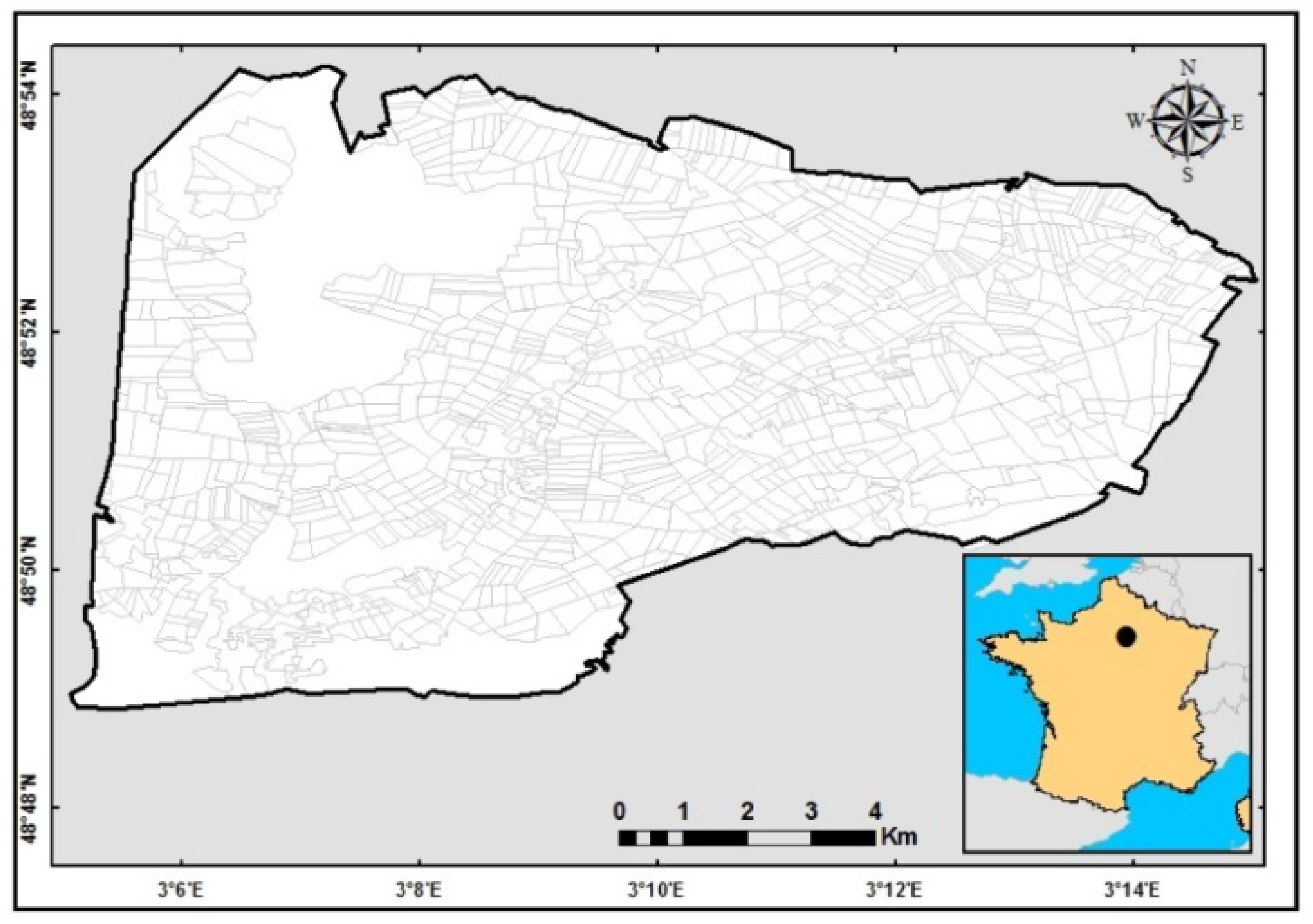
A database of Sentinel-1 (S1) images collected over the Orgeval Basin situated near Paris was used (centered on lat.: 48.86°E and long.: 3.17°N, Figure 1). Relatively flat, the Orgeval Basin is mainly composed of cereal fields (wheat, colza, maize, barley, etc.) and forest. The soil texture is relatively uniform over the whole basin, with clay 20%, silt 70% and sand 10% [29]. Sixty-one S1 images obtained from the Sentinel-1A (S1A) and Sentinel-1B (S1B) satellite constellation operating at the C-band (frequency = 5.406 GHz, wavelength ~6 cm) were collected for the period between 1 November 2016 and 1 March 2017. Over our site, S1A and S1B provide three images every four days, on average. One image is in the Descending mode (acquisition time ~05:58 TU), with an incidence angle of approximately 38°; one is in the Ascending mode (acquisition time ~17:40 TU), with an incidence angle of approximately 42°; and one is in the Ascending mode (acquisition time ~17:31 TU), with an incidence angle of approximately 33°. The 61 S1 images used were acquired in the IW imaging mode with the VV and VH polarizations. In addition, the images were generated from the high-resolution Level-1 Ground Range Detected (GRD) product with a spatial resolution of 10 m × 10 m. These Sentinel-1 images are available via the Copernicus website (https://scihub.copernicus.eu/dhus/#/home). The Sentinel-1 Toolbox (S1TBX), developed by the ESA (European Spatial Agency), was used to calibrate the S1 images. The calibration aims to convert the digital number values of S1 images into backscattering coefficients (σ°) in a linear unit. The radiometric accuracy of Sentinel-1 SAR backscattering coefficient is approximately 0.70 dB (3σ) for the VV polarization and 1.0 dB (3σ) for the VH polarization [30].
A 2017 land cover map based on field trips was used in this study [29]. This map is a thematic vector file with one value per type of land cover. For each vector/segment (one cereal field, one forest stand, etc.), the mean backscattering coefficient was calculated from each calibrated S1 image by averaging the σ° values of all pixels within that vector/segment.
3.2. Temperature Data
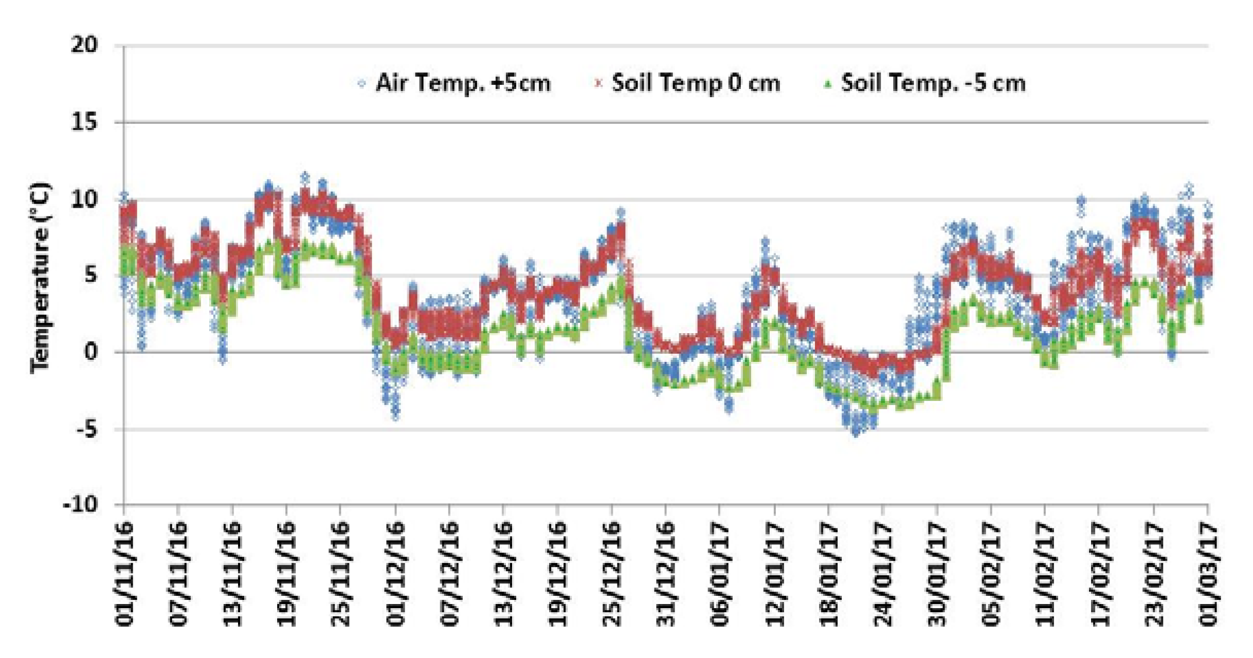
The meteorological data available for our study site describe the air and soil temperatures. The hourly mean air temperature at 5 cm above ground, soil temperature at 5 cm depth, and 0 cm ground surface temperature were used. The continuous temperature series between 1 November 2016 and 1 March 2017 shows three periods with frozen soil conditions, namely 30 November 2016–9 December 2016, 30 December 2016–9 January 2017, and 16 January 2017–31 January 2017, with temperatures that dropped to −5 °C (Figure 2).
4. Results
4.1. Behavior of the Dielectric Constant with the Temperature
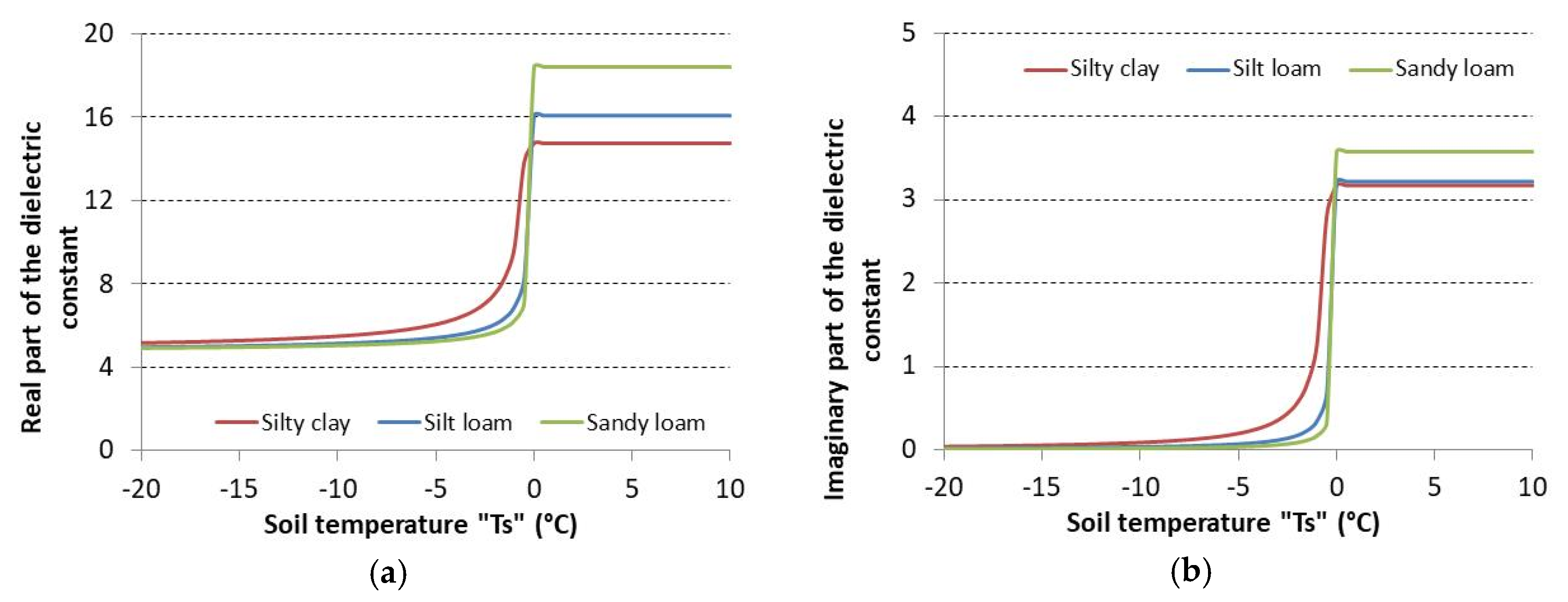
Figure 3 shows the modeling results of the relative dielectric constant of soil (real part , and imaginary part ) at different temperatures for the three typical soils used in this study (Table 1). and increase strongly, especially for temperatures between −5° and 0 °C. The highest difference of the real part of the dielectric constant before and after freezing is approximately 10 for soil of silty clay, 11 for soil silt loam and 13 for soil sandy loam (for soil moisture content of 30 vol%). The imaginary part of the dielectric constant decreases from 3.2 to 0 for silty clay and silt loam soils and from 3.6 to 0 for sandy loam soil.
4.2. Signal Modeling on Frozen Soils
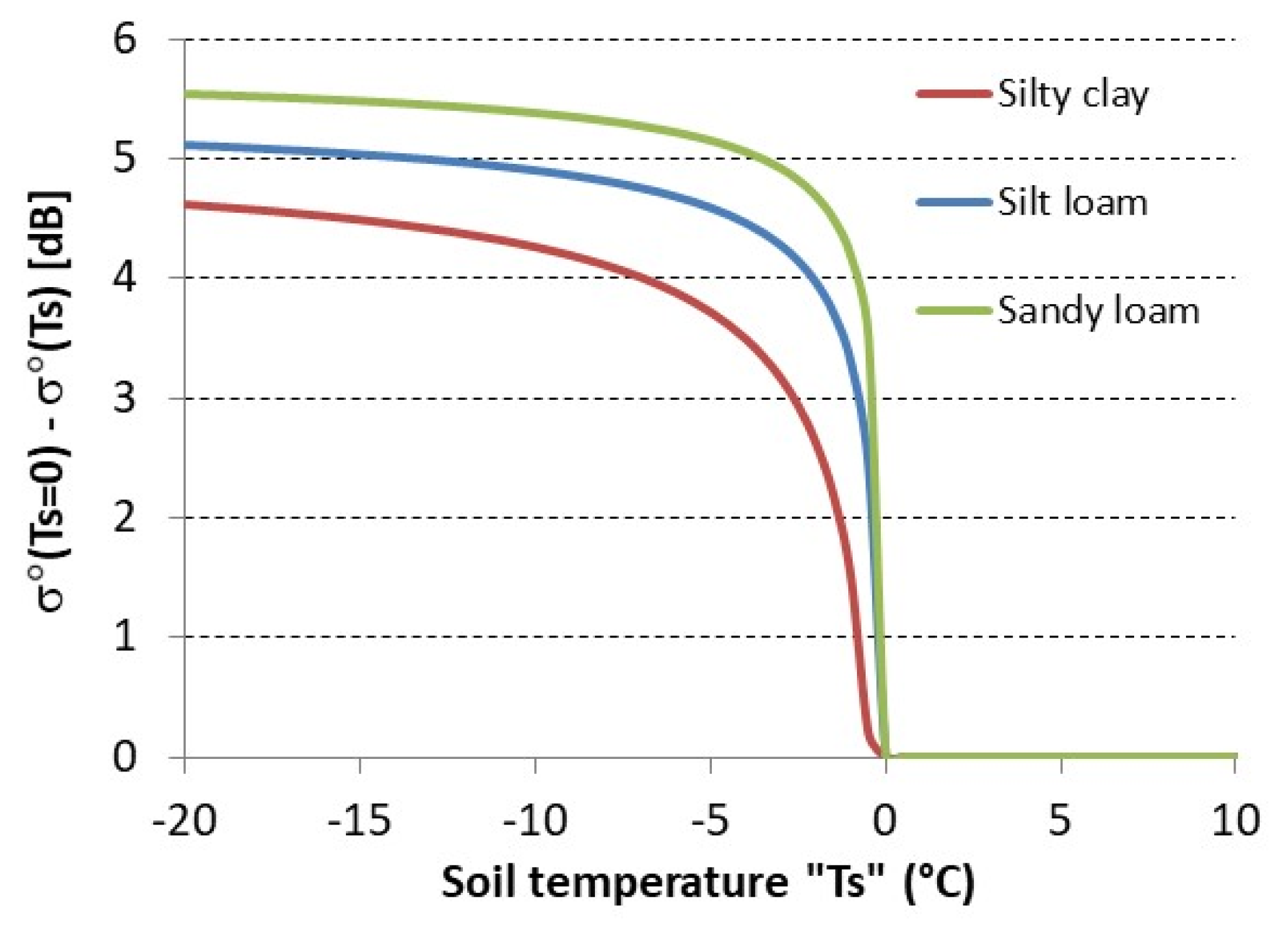
The dielectric constants calculated in Section 4.1 were used in the IEM_B to calculate the backscattering coefficient of the soil surface. Figure 4 shows the difference Δσ° between the backscattering coefficient (σ°) of unfrozen soil that corresponds to a soil temperature higher than 0 °C (in this study the reference soil temperature of unfrozen soil was considered equal to 0 °C) and the backscattering coefficient (σ°) of frozen soil with a temperature between −20 and 0 °C. The maximum difference Δσ° between unfrozen soil and frozen soil is between 4.6 and 5.6 dB depending on the soil type (temperature = −20 °C). For soil with the most clay (silty clay soil type), the difference Δσ° is lower than that for soils with less clay (sandy loam followed by silt loam). For temperatures between −5 and −20 °C, the increase of Δσ° is smaller than 1 dB regardless of soil type. This result in consistent with Figure 3 where the dielectric constant of a frozen soil water mixture increases only slightly with the soil temperature Ts for Ts-values between −20 °C and −5 °C. Figure 4 also shows that, even when the temperature drops to −2 °C, Δσ° ranges between 2.6 and 4.7 dB.
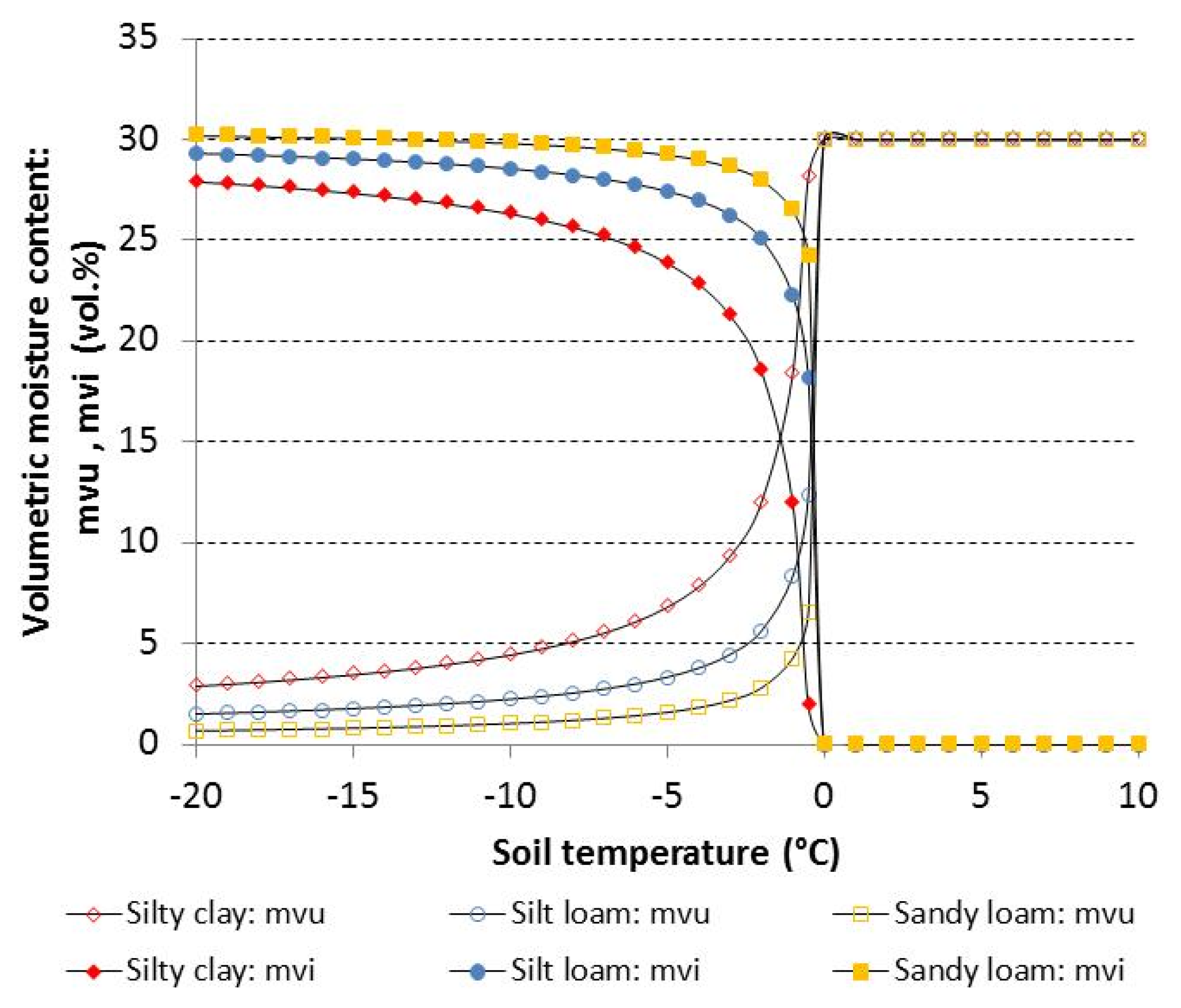
This decrease in the radar signal due to freezing (increase in Δσ°) is more important for sandy soils than for clay soils because sandy soils freeze more quickly than clay soils because of their lesser capacity to store water. To understand the behavior of the radar signal (σ°) with the temperature for the three soil types, the unfrozen volumetric moisture content () and volumetric ice content () were ploted according to the temperature. Figure 5 shows that when there is more clay, the of frozen soil is higher than those of the other soils, and, therefore, σ° is higher. Therefore, σ° for frozen soil with more clay is higher than σ° for frozen soil with less clay. As for all unfrozen soils (whatever the soil type), with more or less clay, σ° is the same since the total volumetric moisture content is the same (in this paper, = 30 vol%) and Δσ° (σ° of frozen soil − σ° of unfrozen soil) for clay soils is lower than Δσ° for soils that are less clay.
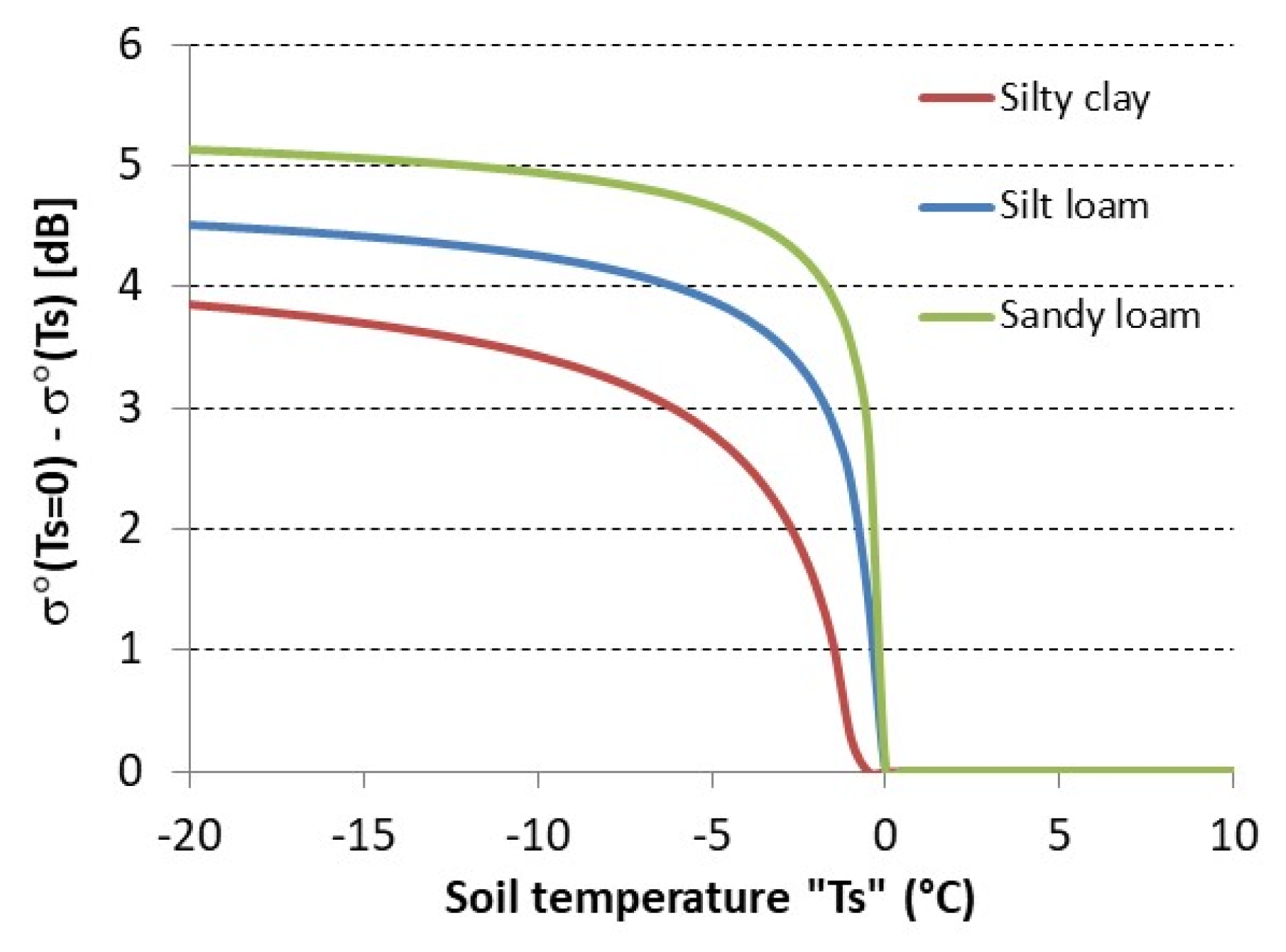
In addition, the effect of the soil moisture value on the potential of the C-band radar signal to discriminate and identify frozen soils was analyzed using a -value of 20 vol%. In comparison with Figure 4 ( = 30 vol%), Figure 6 shows that the potential for discriminating frozen soils slightly decreases when the soil moisture decreases. For mv of 20 vol% and a soil temperature of −20 °C, Δσ° varies between 3.9 and 5.1 dB. Thus, the Δσ° values for = 20 vol% decreased of approximately 0.6 dB (0.7 dB for silty clay and 0.5 dB for sandy loam) compared to Δσ° calculated for = 30 vol%. At −2 °C, Δσ° varies between 1.5 and 4.1 dB, a decrease of approximately 0.9 dB (1.1 dB for silty clay and 0.6 dB for sandy loam) compared to Δσ° calculated with = 30 vol%.
The effect of the Hrms was also investigated using simulations with Hrms = 3 cm (in addition to Hrms = 1 cm). Similar results were obtained concerning the difference Δσ° between the modeled backscattering coefficient of unfrozen soil and the modeled backscattering coefficient of frozen soil.
4.3. Interpretation of Sentinel-1 Images
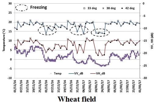
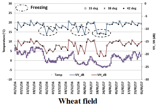
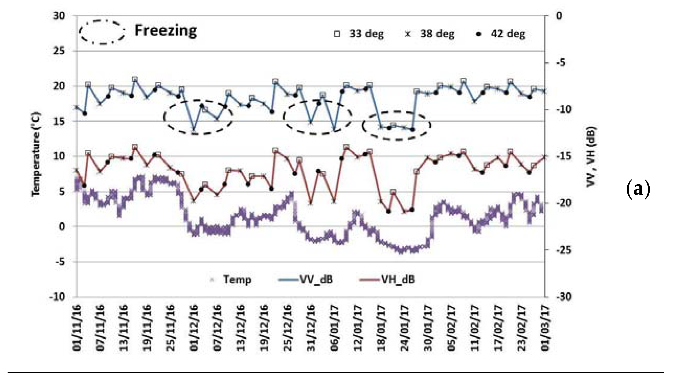
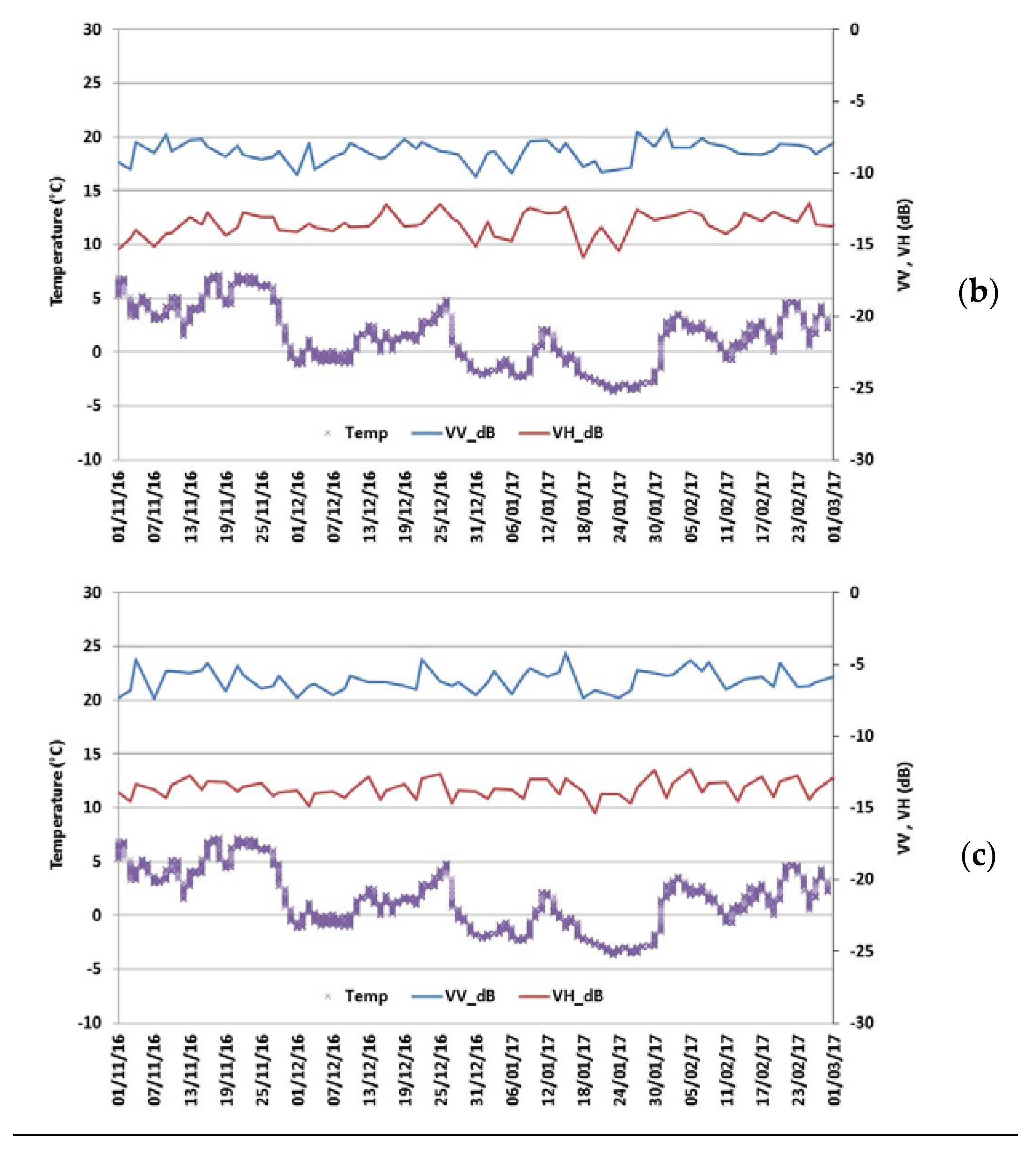
Figure 7 illustrates the temporal behavior for a wheat field, forest stand, and urban area for the Sentinel-1 backscattering coefficient (σ°) in the VV and VH polarizations. For our study site, the vegetation cover of winter crop plots (wheat for example) is relatively low between November and January (height of approximately 5–10 cm). For the wheat field shown in Figure 7a, a decrease in σ°VV of approximately 3–4 dB is observed for the main dates of freezing (soil temperature between −0.6 and −3.7 °C): 1, 7 and 31 December 2016; 6 January 2017; and between 18 and 26 January 2017. In addition, a slight decrease in σ°VV by approximately 1.5 dB is noted on 11 February 2017, when the soil was slightly frozen (soil temperature = −0.6 °C). With VH polarization, the difference between σ° of unfrozen soil and σ° of frozen soil is 1–2 dB higher compared to results obtained in VV polarization, which indicates that the volume scattering strongly influences the cross-polarized signal. Figure 7b shows a slight decrease of the radar signal for the forest stand after a frost episode. This decrease is 3 dB in VH at most (on 18 January 2017) and 2 dB in VV. This decrease of the radar signal corresponds mainly to a decrease of the dielectric constant of ground. The time series of σ° for an urban area logically shows a relatively stable signal independent of frozen soil conditions (Figure 7c).
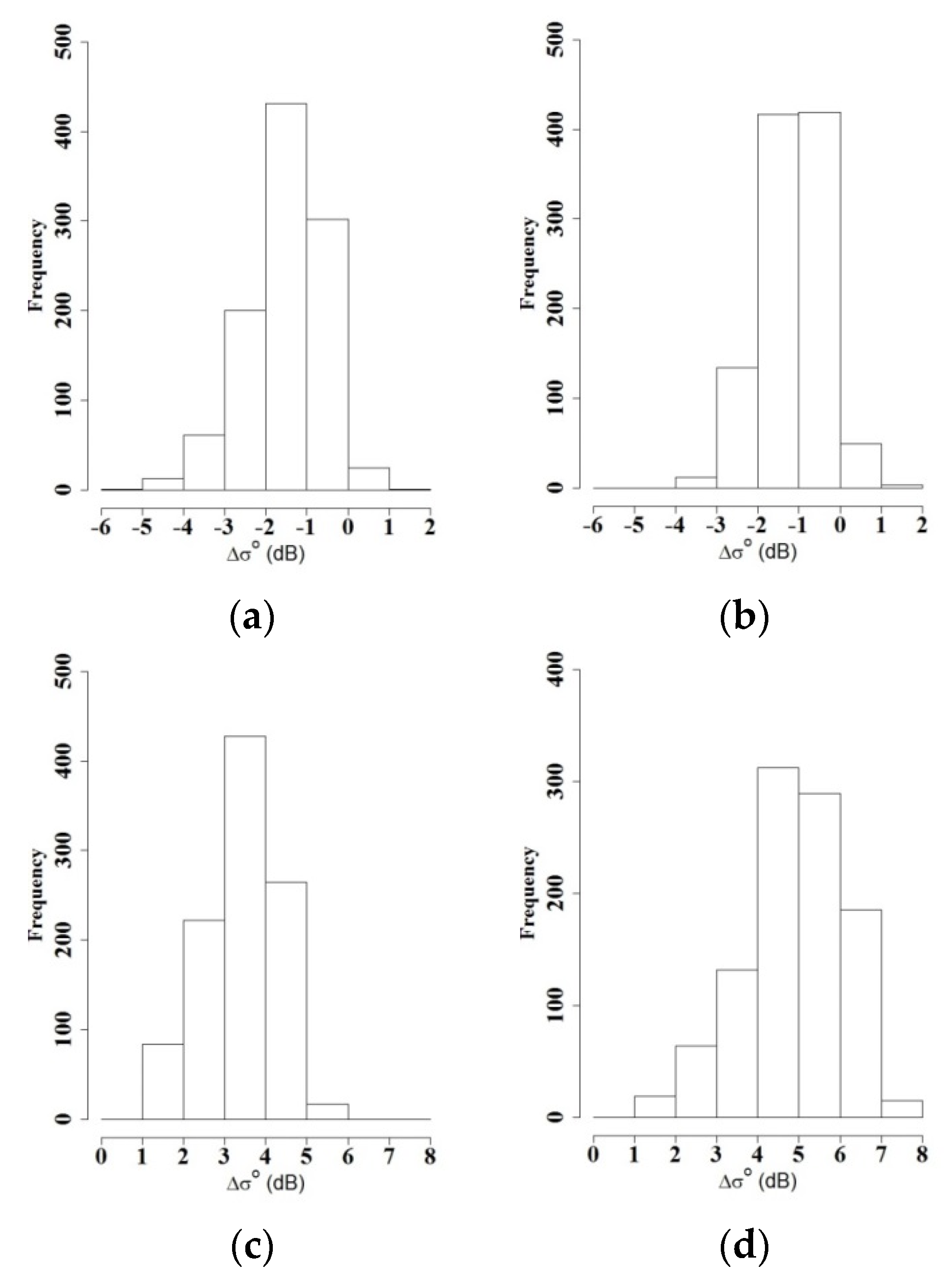
We calculated the difference in Δσ° for all fields corresponding to agricultural land cover (1016 fields) at two dates from Sentinel-1 images (VV and VH), one with an unfrozen soil condition (12 January 2017) and one with a frozen soil condition (18 January 2017). The Δσ° at a given date t = σ° (t0) − σ° (t), where t0 is a date corresponding to the unfrozen soil condition date earlier than t. For a given field, σ° corresponds to the average of σ° of all pixels of the field. The histograms of the difference in Δσ° show that the mean Δσ° on 12 January 2017, is approximately −1.5 dB in VV and −1 dB in VH (Figure 8). For 18 January 2017 (frozen condition), the mean of Δσ° is approximately 3.5 dB in VV and 5 dB in VH. Negative Δσ° values correspond to unfrozen soil and positive Δσ° values correspond to frozen soil. The Δσ° values between −1 and +1 dB are difficult to interpret because the error corresponding to Sentinel-1 radiometric accuracy is approximately 0.70 dB (3σ) for the VV polarization and 1.0 dB (3σ) for the VH polarization [30,31]. Fields with Δσ° values larger than 2 dB have a high probability of being frozen. Higher Δσ° values indicate a robust freezing degree. Figure 8a,b shows negative Δσ° values (or Δσ° < 1 dB) corresponding to unfrozen fields on 12 January 2017 (unfrozen condition). For 18 January 2017 (frozen condition), most fields are detected from Sentinel-1 data as frozen (Figure 8c,d) with better identification using VH polarization (most fields have Δσ° > 2 dB).
4.4. Frozen Soil Mapping
Analysis of the results from the previous sections shows that, when the soil temperature is below 0 °C, there is a significant difference in the radar signal compared to the radar signal with temperatures above 0 °C. Therefore, a simple approach can be proposed for frozen soil mapping. The approach is based on the difference in Δσ° for each field of the agricultural land cover between one image acquired under an unfrozen soil condition and one image acquired under a frozen condition. The date of the image under the non-freezing condition was acquired prior to that of the image acquired under the freezing condition. A difference greater than 2 dB corresponds to a frozen soil. In this approach, we assumed that soil surface roughness is constant between the dates used to calculate Δσ°.
Since the different images are not necessarily acquired at the same incidence angle (images in ascending/descending mode, with different strip map beams), it is necessary to reduce the incidence angle effect by normalizing the backscattering coefficients σ° by a function that represents the angular dependence. Consequently, the backscattering coefficient acquired at an incidence angle θ can be normalized to a fixed reference angle θref (for example 40°) using the following equation [32,33]:
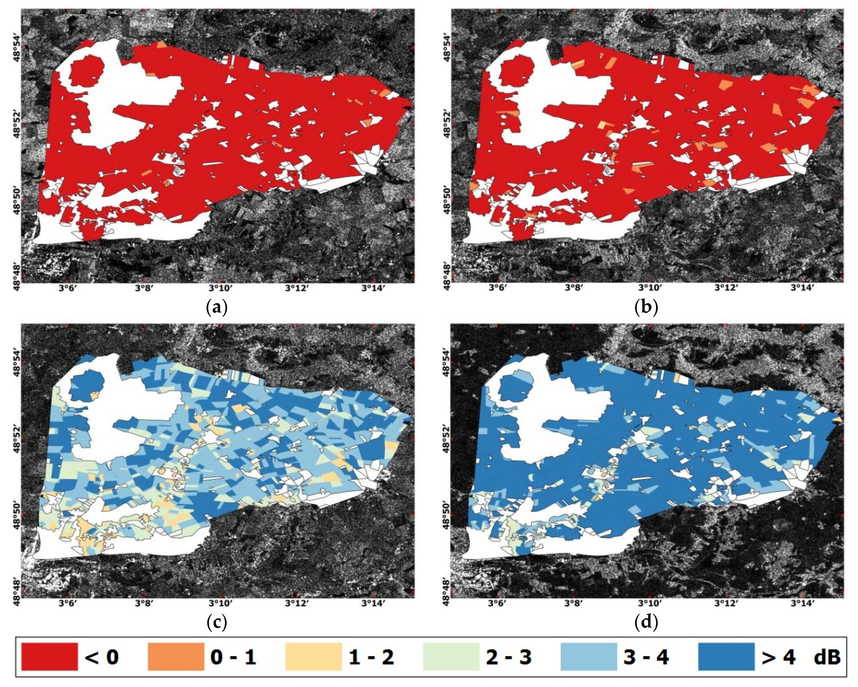
Surface frozen soil maps were built for all available dates. Figure 9 shows the presence or absence of frozen soils for one date with a frozen soil condition and another date with an unfrozen soil condition. A mask was applied to exclude forest and urban areas, as well as mixed land cover (urban + agriculture or forest + agriculture). The maps do not show the presence of frozen soils on 12 January 2017, using VV or VH polarizations (Figure 9a,b), which is consistent with the temperature data. Figure 9c,d shows our basin in a frozen soil condition on 18 January 2017, with better identification of frozen fields with VH polarization (Δσ° higher than 3 dB).
For mapping frozen soils in an operational way, it is possible to classify the fields into three categories: (1) unfrozen soils for Δσ° values lower than 2 dB; (2) soils touched by freezing for Δσ° between 2 and 3; and (3) extremely frozen for fields with Δσ° higher than 3.
5. Discussion
Mapping of frozen soils has some limitations. The presence of snow can lead to poor mapping. If the soil at the acquisition date of the image considered under an unfrozen soil condition is covered with wet snow (temperatures above 0 °C), the radar signal will be at least 3 dB lower [34] compared to the signal for snow-free surfaces or dry snow, which will cause confusion with the signal of a frozen soil and therefore will make it impossible to detect frozen soils. Thus, the difference between an image under a freezing condition and an image without frost but with wet snow will be quite small. The presence of dry snow on the reference image (unfrozen condition) does not lead to the misidentification of frozen soils because the backscatter is relatively high for dry snow or snow-free surfaces, whereas the backscatter can be 3 dB lower for wet snow.
In this study, we assumed that the soil roughness does not change over time. If the roughness of some fields increases on the frost date, then in this case, the difference Δσ° (σ° with freezing and with high roughness, and σ° without freezing with low roughness) will decrease and there may be poor detection of frozen soils. On the other hand, if the roughness decreases between the date of the image without freezing and the date of the image with freezing, the identification of frozen soils will be easier because the decrease of roughness on the date of the image with freezing will increase the signal difference Δσ° (σ° with freezing and with low roughness, and −σ° without freezing with high roughness).
To minimize the effect of a roughness change or the presence of snow on a date, the mapping frozen soils algorithm can use the average of all images acquired in an unfrozen condition before the acquisition date of the image to be analyzed under a freezing condition.
If the soil volumetric moisture content mv increases between the date of the image acquired without freezing and the date of the image under freezing condition, the difference between the radar signal without freezing and the radar signal with freezing should be less than the difference that would have been obtained if there was no rain between the date of the two images. However, if the soil volumetric moisture content decreases between the image dates, the difference between the radar signal for unfrozen soils and the radar signal for frozen soils will be greater than the difference that would have been obtained if there was no drying of the soil between the two images. This soil drying configuration will lead to a negligible decrease in soil moisture content between the two dates because the soil freezing process is mainly observed in winter and the natural soil drying could be assumed low between two images acquired with a few days of lag.
Knowing that the radar signal penetration depth in agricultural area is only a few centimeters at C-band [35], the C-band SAR images provide information on frozen soils only for the top soil surface layer. Thus, the few centimeters of C-band radar signal penetration depth do not allow obtaining information on deep frozen soils.
This study also showed that, for temperatures slightly below 0 °C (around −4 °C), the freeze in forest stands is slightly visible, probably because these areas freeze at much lower temperatures. Rignot et al. [2] observed at 3 dB decrease in the ERS-1 radar signal (C-Band) when the soil and vegetation freeze (air temperature reaches −30 °C).
It is worth mentioning that our study was carried out during the winter season with very low vegetation cover. In the case of more developed vegetation cover, possibly frozen areas mapping could be more difficult especially if the temperature is slightly below 0 °C (signal difference between unfrozen and frozen areas will be lower). Further investigations are necessary to analyze the effect of frozen water content in crop on the SAR backscattering coefficient.
6. Conclusions
This paper investigates, from a semi-empirical dielectric constant model and times series of Sentinel-1 images, the potential of the new C-band SAR Sentinel-1 sensor for classifying frozen/unfrozen soils in an agricultural context.
When the soil temperature decreases, the liquid water content also decreases, and, consequently, the backscattered signal decreases. The results indicate that frozen soils showed a lower radar backscattering signal than the unfrozen soils by approximately 3 dB. A classification of frozen soils using Sentinel-1 images was proposed to identify frozen and unfrozen soils for all crop fields. The method uses the difference between the radar backscattering coefficient of the image acquired at a date without any freezing condition (temperature higher than 0 °C) and the radar backscattering coefficient of acquired image under a frozen condition (temperature lower than 0 °C). Simulations performed from a semi-empirical dielectric constant model show that the difference between frozen soils and unfrozen soils increases when the soil moisture content increases.
If the soil roughness of a given field changes between the acquisition dates of the two images used, the image under a freezing condition and the image under a non-freezing condition, the detection of frozen soils can be problematic. In addition, the presence of wet snow on the image acquired under a non-freezing condition can lead to poor identification of frozen soils.
The results of this study provide an interesting way to map frozen soils using the high spatial and temporal resolutions of Sentinel-1 sensors. The frozen soil maps are of great interest to assess damage in agricultural areas.
Author Contributions
B.N. conceived and designed the experiments; B.N. and B.H. performed the experiments; B.N. and B.H. analyzed the results; B.N. wrote the article; B.H., E.M., and Z.M. revised the paper.
Acknowledgments
This research was supported by IRSTEA (National Research Institute of Science and Technology for Environment and Agriculture) and the French Space Study Center (CNES, TOSCA 2018). Authors thank the European Space Agency that provided the Sentinel-1 data.
Conflicts of Interest
The authors declare no conflict of interest.
References
- Wegmüller, U. The effect of freezing and thawing on the microwave signatures of bare soil. Remote Sens. Environ. 1990, 33, 123–135. [Google Scholar] [CrossRef]
- Rignot, E.; Way, J.B.; McDonald, K.; Viereck, L.; Williams, C.; Adams, P.; Payne, C.; Wood, W.; Shi, J. Monitoring of environmental conditions in taiga forests using ERS-1 SAR. Remote Sens. Environ. 1994, 49, 145–154. [Google Scholar] [CrossRef]
- Khaldoune, J.; Van Bochove, E.; Bernier, M.; Nolin, M.C. Mapping agricultural frozen soil on the watershed scale using remote sensing data. Appl. Environ. Soil Sci. 2011, 2011, 193237. [Google Scholar] [CrossRef]
- Park, S.-E.; Bartsch, A.; Sabel, D.; Wagner, W.; Naeimi, V.; Yamaguchi, Y. Monitoring freeze/thaw cycles using ENVISAT ASAR Global Mode. Remote Sens. Environ. 2011, 115, 3457–3467. [Google Scholar] [CrossRef]
- Jagdhuber, T.; Stockamp, J.; Hajnsek, I.; Ludwig, R. Identification of soil freezing and thawing states using SAR polarimetry at C-band. Remote Sens. 2014, 6, 2008–2023. [Google Scholar] [CrossRef]
- Baghdadi, N.; Cerdan, O.; Zribi, M.; Auzet, V.; Darboux, F.; El Hajj, M.; Kheir, R.B. Operational performance of current synthetic aperture radar sensors in mapping soil surface characteristics in agricultural environments: application to hydrological and erosion modelling. Hydrol. Process. 2008, 22, 9–20. [Google Scholar] [CrossRef]
- Derksen, C.; Xu, X.; Dunbar, R.S.; Colliander, A.; Kim, Y.; Kimball, J.S.; Black, T.A.; Euskirchen, E.; Langlois, A.; Loranty, M.M. Retrieving landscape freeze/thaw state from Soil Moisture Active Passive (SMAP) radar and radiometer measurements. Remote Sens. Environ. 2017, 194, 48–62. [Google Scholar] [CrossRef]
- Baghdadi, N.; Holah, N.; Zribi, M. Calibration of the integral equation model for SAR data in C-band and HH and VV polarizations. Int. J. Remote Sens. 2006, 27, 805–816. [Google Scholar] [CrossRef]
- Baghdadi, N.; Chaaya, J.A.; Zribi, M. Semiempirical calibration of the integral equation model for SAR data in C-band and cross polarization using radar images and field measurements. IEEE Geosci. Remote Sens. Lett. 2011, 8, 14–18. [Google Scholar] [CrossRef]
- Dobson, M.C.; Ulaby, F.T.; Hallikainen, M.T.; El-Rayes, M.A. Microwave dielectric behavior of wet soil-Part II: Dielectric mixing models. IEEE Trans. Geosci. Remote Sens. 1985, 1, 35–46. [Google Scholar] [CrossRef]
- Peplinski, N.R.; Ulaby, F.T.; Dobson, M.C. Dielectric properties of soils in the 0.3–1.3-GHz range. IEEE Trans. Geosci. Remote Sens. 1995, 33, 803–807. [Google Scholar] [CrossRef]
- Stogryn, A. Equations for calculating the dielectric constant of saline water (correspondence). IEEE Trans. Microw. Theory Tech. 1971, 19, 733–736. [Google Scholar] [CrossRef]
- Ulaby, F.T.; Moore, R.K.; Fung, A.K. Microwave Remote Sensing: Active and Passive, Vol. III, Volume Scattering and Emission Theory, Advanced Systems and Applications; Artech House Inc.: Dedham, MD, USA, 1986; pp. 1797–1848. [Google Scholar]
- Zhang, L.; Shi, J.; Zhang, Z.; Zhao, K. The estimation of dielectric constant of frozen soil-water mixture at microwave bands. In Proceedings of the 2003 IEEE International Geoscience and Remote Sensing Symposium, Toulouse, France, 21–25 July 2003; Volume 4, pp. 2903–2905. [Google Scholar]
- Zribi, M.; Baghdadi, N.; Holah, N.; Fafin, O.; Guérin, C. Evaluation of a rough soil surface description with ASAR-ENVISAT radar data. Remote Sens. Environ. 2005, 95, 67–76. [Google Scholar] [CrossRef]
- Baghdadi, N.; Aubert, M.; Zribi, M. Use of TerraSAR-X data to retrieve soil moisture over bare soil agricultural fields. IEEE Geosci. Remote Sens. Lett. 2012, 9, 512–516. [Google Scholar] [CrossRef] [Green Version]
- Le Morvan, A.; Zribi, M.; Baghdadi, N.; Chanzy, A. Soil moisture profile effect on radar signal measurement. Sensors 2008, 8, 256–270. [Google Scholar] [CrossRef] [PubMed]
- El Hajj, M.; Baghdadi, N.; Belaud, G.; Zribi, M.; Cheviron, B.; Courault, D.; Hagolle, O.; Charron, F. Irrigated grassland monitoring using a time series of terraSAR-X and COSMO-skyMed X-Band SAR Data. Remote Sens. 2014, 6, 10002–10032. [Google Scholar] [CrossRef] [Green Version]
- El Hajj, M.; Baghdadi, N.; Zribi, M.; Bazzi, H. Synergic use of Sentinel-1 and Sentinel-2 images for operational soil moisture mapping at high spatial resolution over agricultural areas. Remote Sens. 2017, 9, 1292. [Google Scholar] [CrossRef]
- Choker, M.; Baghdadi, N.; Zribi, M.; El Hajj, M.; Paloscia, S.; Verhoest, N.E.; Lievens, H.; Mattia, F. Evaluation of the Oh, Dubois and IEM Backscatter Models Using a Large Dataset of SAR Data and Experimental Soil Measurements. Water 2017, 9, 38. [Google Scholar] [CrossRef]
- Fung, A.K. Microwave Scattering and Emission Models and Their Applications; Artech House Inc.: Boston, MA, USA, 1994; ISBN 978-0-89006-523-5. [Google Scholar]
- Panciera, R.; Tanase, M.A.; Lowell, K.; Walker, J.P. Evaluation of IEM, Dubois, and Oh radar backscatter models using airborne L-band SAR. IEEE Trans. Geosci. Remote Sens. 2014, 52, 4966–4979. [Google Scholar] [CrossRef]
- Gorrab, A.; Zribi, M.; Baghdadi, N.; Mougenot, B.; Fanise, P.; Chabaane, Z.L. Retrieval of both soil moisture and texture using TerraSAR-X images. Remote Sens. 2015, 7, 10098–10116. [Google Scholar] [CrossRef] [Green Version]
- Baghdadi, N.; Saba, E.; Aubert, M.; Zribi, M.; Baup, F. Evaluation of Radar Backscattering Models IEM, Oh, and Dubois for SAR Data in X-Band Over Bare Soils. IEEE Geosci. Remote Sens. Lett. 2011, 8, 1160–1164. [Google Scholar] [CrossRef]
- Baghdadi, N.; King, C.; Chanzy, A.; Wigneron, J.P. An empirical calibration of the integral equation model based on SAR data, soil moisture and surface roughness measurement over bare soils. Int. J. Remote Sens. 2002, 23, 4325–4340. [Google Scholar] [CrossRef]
- Baghdadi, N.; Zribi, M.; Paloscia, S.; Verhoest, N.E.; Lievens, H.; Baup, F.; Mattia, F. Semi-empirical calibration of the integral equation model for co-polarized L-band backscattering. Remote Sens. 2015, 7, 13626–13640. [Google Scholar] [CrossRef] [Green Version]
- Baghdadi, N.; Saba, E.; Aubert, M.; Zribi, M.; Baup, F. Comparison between backscattered TerraSAR signals and simulations from the radar backscattering models IEM, Oh, and Dubois. IEEE Geosci. Remote Sens. Lett. 2011, 6, 1160–1164. [Google Scholar] [CrossRef]
- Baghdadi, N.; Zribi, M. Characterization of Soil Surface Properties Using Radar Remote Sensing. In Land Surface Remote Sensing in Continental Hydrology; Elsevier: Oxford, UK, 2016; pp. 1–39. [Google Scholar]
- Tallec, G.; Ansart, P.; Guérin, A.; Delaigue, O.; Blanchouin, A. Observatoire Oracle. Available online: http://dx.doi.org/10.17180/OBS.ORACLE (accessed on 25 May 2015).
- Schwerdt, M.; Schmidt, K.; Tous Ramon, N.; Klenk, P.; Yague-Martinez, N.; Prats-Iraola, P.; Zink, M.; Geudtner, D. Independent System Calibration of Sentinel-1B. Remote Sens. 2017, 9, 511. [Google Scholar] [CrossRef]
- El Hajj, M.; Baghdadi, N.; Zribi, M.; Angelliaume, S. Analysis of Sentinel-1 Radiometric Stability and Quality for Land Surface Applications. Remote Sens. 2016, 8, 406. [Google Scholar] [CrossRef] [Green Version]
- Baghdadi, N.; Bernier, M.; Gauthier, R.; Neeson, I. Evaluation of C-band SAR data for wetlands mapping. Int. J. Remote Sens. 2001, 22, 71–88. [Google Scholar] [CrossRef]
- Topouzelis, K.; Singha, S.; Kitsiou, D. Incidence angle normalization of Wide Swath SAR data for oceanographic applications. Open Geosci. 2016, 8, 450–464. [Google Scholar] [CrossRef]
- Baghdadi, N.; Gauthier, Y.; Bernier, M. Capability of multitemporal ERS-1 SAR data for wet-snow mapping. Remote Sens. Environ. 1997, 60, 174–186. [Google Scholar] [CrossRef]
- Ulaby, F.T.; Moore, R.K.; Fung, A.K. Microwave Remote Sensing Active and Passive-Volume III: From Theory to Applications; Artech House Inc.: Norwood, MA, USA, 1986. [Google Scholar]
Figure 1.
Location of the study site.

Figure 2.
Air (at 5 cm) and soil temperatures (ground surface and at 5 cm depth). Temperature was recorded using HOBO U12 sensors.
Figure 2.
Air (at 5 cm) and soil temperatures (ground surface and at 5 cm depth). Temperature was recorded using HOBO U12 sensors.

Figure 3.
Dielectric constant of a frozen soil–water mixture according to the soil temperature for three soil types (Table 1): (a) real part ; and (b) imaginary part . = 30 vol%, = 1 g/cm3, = 0.9175 g/cm3, and A, B and are given in Table 1.

Figure 4.
Difference Δσ° between the modeled backscattering coefficient of unfrozen soil with reference temperature Ts equal to 0 °C “σ° (Ts = 0°)” and the modeled backscattering coefficient of frozen soil with soil temperature between −20 °C and 0 °C “σ° (Ts)”. For soil temperatures above 0 °C, Δσ° (σ° (Ts = 0) − σ° (Ts > 0°)) is equal to 0 dB. Radar frequency f = 5.405 GHz, = 30 vol%, Hrms = 1 cm, incidence angle θ = 40°, and polarization = VV.

Figure 5.
Unfrozen volumetric moisture content () and corresponding volumetric ice content ( ) of soil during freezing according to the soil temperature for three soil types (Table 1). = 30 vol%, = 1 g/cm3, = 0.9175 g/cm3, A, B and are given in Table 1.

Figure 6.
Difference in Δσ° between the modeled backscattering coefficient of unfrozen soil with reference temperature Ts equal to 0 °C “σ° (Ts = 0°)” and the modeled backscattering coefficient of frozen soil with soil temperature between −20 °C and 10 °C “σ° (Ts)”. Frozen soils correspond to Ts lower than 0 °C. Radar frequency f = 5.405 GHz, = 20 vol%, Hrms = 1 cm, incidence angle θ = 40°, and polarization = VV.

Figure 7.
Temporal variation for the Sentinel-1 backscattering coefficient σ° between 1 November 2016, and 3 March 2017 for: (a) a wheat reference field; (b) a forest stand; and (c) an urban area. The soil temperature at a 5 cm depth is also plotted.
Figure 7.
Temporal variation for the Sentinel-1 backscattering coefficient σ° between 1 November 2016, and 3 March 2017 for: (a) a wheat reference field; (b) a forest stand; and (c) an urban area. The soil temperature at a 5 cm depth is also plotted.


Figure 8.
Histograms of the difference in Δσ° for two dates calculated from Sentinel-1 images, one with an unfrozen soil condition (12 January 2017) and one with a frozen soil condition (18 January 2017): (a) 12 January 2017, VV polarization; (b) 12 January 2017, VH polarization; (c) 18 January 2017, VV polarization; and (d) 18 January 2017, VH polarization. Δσ° at a given date t = σ° (t0) − σ° (t), where t0 is a date corresponding to an unfrozen soil condition date earlier than t.

Figure 9.
Maps of the frozen/unfrozen soil conditions: one date (12 January 2017) in an unfrozen soil condition (a,b); and one date (18 January 2017) corresponding to a frozen soil condition (c,d). Only crop fields were considered: (a,c) using VV; and (b,d) using VH. The mask in white corresponds to forest stands, urban areas and some mixed land cover (urban + agriculture or forest + agriculture).


Table 1.
Coefficients A and B derived for three soil types by Zhang et al. [14].
Table 1.
Coefficients A and B derived for three soil types by Zhang et al. [14].
| Soil Type | Soil Texture (%) | ρb | ρs | A | B | ||
|---|---|---|---|---|---|---|---|
| Sand | Silt | Clay | |||||
| Silty-clay | 6.83 | 45.76 | 47.41 | 1.62 | 2.60 | 11.3301 | 0.6166 |
| Silt-loam | 28.58 | 51.46 | 19.96 | 1.58 | 2.58 | 5.2752 | 0.5675 |
| Sandy-loam | 50.73 | 39.61 | 9.66 | 1.59 | 2.63 | 2.6945 | 0.6104 |
© 2018 by the authors. Licensee MDPI, Basel, Switzerland. This article is an open access article distributed under the terms and conditions of the Creative Commons Attribution (CC BY) license (http://creativecommons.org/licenses/by/4.0/).
Share and Cite
MDPI and ACS Style
Baghdadi, N.; Bazzi, H.; El Hajj, M.; Zribi, M. Detection of Frozen Soil Using Sentinel-1 SAR Data. Remote Sens. 2018, 10, 1182. https://doi.org/10.3390/rs10081182
AMA Style
Baghdadi N, Bazzi H, El Hajj M, Zribi M. Detection of Frozen Soil Using Sentinel-1 SAR Data. Remote Sensing. 2018; 10(8):1182. https://doi.org/10.3390/rs10081182
Chicago/Turabian StyleBaghdadi, Nicolas, Hassan Bazzi, Mohammad El Hajj, and Mehrez Zribi. 2018. "Detection of Frozen Soil Using Sentinel-1 SAR Data" Remote Sensing 10, no. 8: 1182. https://doi.org/10.3390/rs10081182
Note that from the first issue of 2016, this journal uses article numbers instead of page numbers. See further details here.