Prediction of Mud Pressures for the Stability of Wellbores Drilled in Transversely Isotropic Rocks


DIATI Politecnico di Torino, corso Duca degli Abruzzi 24, 10129 Torino, Italy
*
Author to whom correspondence should be addressed.
Energies 2018, 11(8), 1944; https://doi.org/10.3390/en11081944
Submission received: 11 May 2018
/
Revised: 12 July 2018
/
Accepted: 21 July 2018
/
Published: 26 July 2018
(This article belongs to the Section L: Energy Sources)
Abstract
:Serious borehole instability problems are often related to the presence of weakness planes in rock formations. In this study, we investigated the stability of wellbores drilled along a principal direction and parallel to the weakness planes. We used three different strength criteria (weakness plane model, Hoek and Brown and Nova and Zaninetti) to calculate the mud pressures to avoid slip and tensile failure along the weakness planes. We identified the orientation of the weakness planes that generate the most critical slip condition as a function of the friction angle of the planes. We also identified the range of orientations of the weakness planes that corresponds with the lower mud pressure window. We confirmed the validity of the proposed relationships with comparative stability analyses by using analytical solutions and numerical simulations (Ubiquitous Joint Model, FLAC). We found that the mud pressures calculated with the Hoek and Brown criterion show a particular trend, which cannot be predicted by the weakness plane model. We provided two normalized stability charts to predict mud pressures to prevent slip along the weakness planes in the critical slip condition. Finally, we corroborated our findings by simulating the stability of wellbores drilled in the Pedernales Field (Venezuela) and in oil fields located in Bohai Bay (China).
1. Introduction
Maintaining stability in a wellbore during drilling operations is still a matter of concern for the oil and gas industry, because instability can increase drilling costs [1].
Wellbores drilled to access reservoirs go through different rocks that can contain discontinuities, from faults at large scale to thinly laminated planes at small scale [2]. In particular, wellbores drilled in shales can experience serious instabilities related to sliding along the bedding planes.
Last and Mc Lean [3], Twynam et al. [4], and Willson et al. [5] analyzed wellbore failure in the Cusiana Field (Colombia) and the Pedernales Field (Venezuela). Instability occurred when drilling in the intra-reservoir shales, which are characterized by fissility and natural fractures. They found that stability improved by raising mud pressure, and when the wellbore axis was nearly normal to the bedding planes (up-dip), while drilling down-dip and cross-dip resulted in serious instability.
Oakland and Cook [6] investigated wellbore instabilities in the Osenberg Field (North Sea). Instability problems were experienced in the Draupne formation, which is fissile shale. Based on field experience, they concluded that stability improved when the wellbore trajectory was normal to the bedding planes, while serious instability resulted when the hole axis was parallel to bedding.
Brehm et al. [7] reported wellbore instabilities in the Shenzi Field (Gulf of Mexico), characterized by weakly bedded rocks. They observed that while drilling the first wells, instability grew when drilling down-dip at low attack angles, but was almost non-existent when drilling up-dip (nearly normal to the bedding planes). Ultimately, they noticed lost circulation when mud pressures were raised to avoid instability in the wellbores drilled down-dip.
Wu and Tan [8] noticed serious instability problems in an oil field in Bohai Bay (China) when drilling at high angles (deviations in excess to 60°), and when drilling horizontal wells in shales characterized by nearly horizontal bedding planes. Vertical or sub-vertical wellbores experienced minor drilling problems.
Narayanasamy et al. [9] reported wellbore instabilities in the Clair Oilfield (West of Shetlands, UK), characterized by cretaceous mudstones with bedding planes. They noticed that wellbores drilled with the axis nearly parallel to the weakness planes experienced serious problems. Based on this experience, a wellbore was drilled successfully by raising the mud pressure. However, the authors observed that the required mud pressure to avoid slip was close to the tensile fracturing pressure of the mudstones.
This field evidence allowed us to realize wellbore stability changes with variations of the angle between the wellbore axis and the weakness planes. Wellbores drilled parallel to the weakness planes required the highest mud pressures to avoid slip. However, these high mud pressures can result in mud leakage or even lost circulation.
Stability analyses of wellbores drilled in these fields were carried out with software based on the weakness plane model [10]. This model is largely used in the oil and gas industry for the prediction of mud pressures to avoid slip ([4,5,6,7,8,9,11,12,13,14,15,16,17,18,19,20,21]).
The prediction of the fracture pressure in wellbores drilled in transversely isotropic rocks has received less attention due to the difficulty related to the experimental validation of the tensile criteria proposed in the literature [22]. Ma et al. [22,23,24] analyzed the results of tensile direct and indirect tests which were carried out on transversely isotropic rocks, and performed a comparative analysis by interpreting the experimental data with different strength criteria: Hobbs and Barron [25,26], Nova and Zaninetti [27], and Single Plane of Weakness [28]. They found that the Nova and Zaninetti (1990) criterion matches the experimental data quite well [22]. They also set up a stability analysis to avoid fracturing in synthetic cases.
It is well known that experimental strength data are not always appropriately matched by the weakness plane model [21], in particular in the range of inclinations described by the plateau of constant strength. Transversely isotropic rocks can exhibit strength patterns, which are different from the predicted constant strength. A comparative analysis of the match of experimental data with the weakness plane model and another criterion is needed for proper prediction of mud pressures.
We selected six different rocks and interpreted the triaxial tests performed on them with the weakness plane model and the Hoek and Brown criterion [29], adapted to rocks affected by strength anisotropy [30,31].
Although wellbores drilled parallel to the weakness planes require the highest mud pressures, we noted there was a lack of a detailed study of the different stability scenarios related to the inclinations of the planes in the cross section normal to the wellbore axis (Figure 1).
We investigated the stability of wellbores drilled along a principal direction and parallel to the weakness planes by varying the inclination δ (Figure 1) of the weakness planes, using the data of the six rocks. We performed comparative stability analyses with the weakness plane model and the Hoek and Brown criterion adapted to rocks with strength anisotropy. To our knowledge, the Hoek and Brown criterion has not yet been used in stability analyses of wellbores drilled in rocks affected by strength anisotropy. In some cases, the mud pressures calculated with the Hoek and Brown criterion yielded different results from those calculated with the weakness plane model.
We identified a critical inclination of the weakness planes that requires the highest mud pressure to prevent slip. We confirmed our result by performing numerical runs with the Ubiquitous Joint Model implemented in Fast Lagrangian Analysis of Continua (FLAC) (version 6, Itasca Consulting Group, Inc., Minneapolis, MN, USA). Furthermore, as the inclination δ of the weakness planes can vary over relatively short sections of the wellbore [5,7], we identified a reference mud pressure to be used in cases where there are geological uncertainties.
On the other hand, we needed to verify if these high mud pressures could cause the occurrence of tensile failure (fracturing). We investigated this aspect by using the results of Brazilian tests performed on two rocks. We interpreted these results with the Nova and Zaninetti criterion, and we defined the mud pressure windows (i.e., the difference between the mud pressure to avoid tensile fracturing and the mud pressure to avoid slip) for all the inclinations δ of the weakness planes.
For practical purposes, we set up two normalized stability charts. Finally, we applied our findings to analyze the stability of wellbores drilled in the Pedernales Field (Venezuela) and in oil fields located in Bohai Bay (China).
2. Selection of Strength Criteria for Rocks with Strength Anisotropy Related to the Weakness Planes
Anisotropic rocks exhibit different properties in different directions. Several experimental studies ([22,23,24,31,32,33,34,35,36,37,38,39,40,41]) indicate that the majority of sedimentary and metamorphic rocks are affected by strength anisotropy related to discontinuities. The results of triaxial tests and direct and indirect tensile tests carried out on these rocks show that strength changes with loading orientation. Consequently, the prediction of the strength of these rocks must be carried out with criteria that account for the presence of these weakness planes.
We can subdivide the criteria formulated for transversely isotropic rocks into two main types: discontinuous models and continuous models. In discontinuous models, there is a distinction between slip along the planes and failure in the rock matrix. Thus, the strength of the rock matrix is constant with orientation if slip does not occur along the weakness planes, whereas it changes with the orientation of the planes if slip failure occurs. On the other hand, continuous models consider ongoing variation in strength with all the possible orientations of the planes. In these models, there is no implicit distinction between failure on the weakness planes and failure in the rock matrix [34].
The pioneering strength criterion for anisotropic rocks is the Jaeger’s plane of weakness model [10]. This model is based on the Coulomb criterion, and considers two independent failure modes: failure along the discontinuity and failure through the intact rock material. This criterion was modified by Jaeger [42] and McLamore and Gray [37] by introducing the variation of the strength with the inclination of the weakness planes. Walsh and Brace [43] modified the Griffith criterion by assuming that the weak planes consist of a set of parallel elliptical cracks. Nonetheless, these models have not received particular attention from either the scientific or the technical communities.
In order to predict the strength of intact anisotropic rocks, Hoek and Brown [29] suggested that the value of the constants of their empirical nonlinear criterion should change with the orientation of the weakness planes. Recently, Tien and Kuo [30] and Colak & Unlu [31] have modified this criterion by assuming that the rock is intact and instantaneously isotropic at every inclination of the weakness planes.
For our purposes, we selected the weakness plane model which is linear and characterized by two constant strength parameters: the cohesion and the friction angle of the weakness planes. To date, the weakness plane model seems to be the most widely used for predicting mud pressures in wellbores drilled in anisotropic rocks ([4,5,6,7,8,9,11,12,13,14,15,16,17,18,19,20]). This is probably because the cohesion and the friction angle of the discontinuities can be directly determined by direct shear tests. However, this criterion predicts a constant strength for a range of inclinations of the weakness planes, which is not always present in the experimental strength data.
We selected the Hoek and Brown criterion adapted to rocks with anisotropic strength [30,31] for a more accurate account of the experimental results. The Hoek and Brown criterion has been applied successfully to a wide range of intact and fractured rock types [44,45] by practitioners in rock engineering for over 30 years. The use of the Hoek and Brown criterion in petroleum engineering is not common because of the uncertainties related to the determination of the controlling parameters. However, some authors applied this criterion to evaluate the stability of wellbores drilled in isotropic rocks. In general, the results of these analyses show a good match between field evidence and calculated mud pressures ([46,47,48,49,50]).
The application of the Hoek and Brown criterion to rocks with anisotropic strength requires the determination of the controlling parameters at various inclinations of the weakness planes, making the analysis a hard job. To our knowledge, this criterion has not yet been used in stability analyses of wellbores drilled in rocks affected by weakness planes, most likely because of the high number of triaxial tests required to characterize rock strength.
Ultimately, we adopted the Nova and Zaninetti criterion to investigate the occurrence of tensile failure. We selected this criterion because it matches quite well with the results of direct tensile tests and Brazilian tests [22].
We briefly describe the criteria that we used for the wellbore stability analyses below.
2.1. The Weakness Plane Model and the Ubiquitous Joint Model (FLAC)
Jaeger [10] modeled a rock containing well-defined parallel planes of weakness by considering that each plane has a limiting shear strength defined by the Coulomb criterion:
where c’w and φ’w are the cohesion and the friction angle respectively of the weakness planes.
We consider an element subject to a principal state of stress σ1 and σ3 containing weakness planes with an inclination βw (Figure 2a). Combining Equation (1) with the stress transformation equations (Appendix A), it is possible to find the limit condition for sliding along these planes (weakness plane model):
Equation (2) exhibits a minimum when βw = 45° + φ’w/2. For values of βw approaching 90° and in the range 0° to φ’w, slip cannot occur on the plane of weakness. Within these ranges, the criterion considers a plateau of constant strength.
The weakness plane model is classified as a discontinuous criterion and is based on the constant value of the friction angle, cohesion along the weakness planes, and a constant strength plateau for the rock matrix. The cohesion and the friction angle of the weak planes are calculated from laboratory tests at βw = 45° + φ’w/2. The variation of the strength with the inclination depends only on the variation of the angle βw by means of Equation (2). The weakness plane model is a simple criterion that accounts for neither the complex patterns of discontinuities nor the occurrence of a combination of slip and failure in the rock matrix which was observed in laboratory tests ([41]).
In the Ubiquitous Joint Model implemented in FLAC, yield can occur in either the solid or along the weakness planes, or both, depending on the stress state, orientation of the planes, and material properties of the solid and weakness plane. The criterion for failure in the rock matrix is the Mohr Coulomb model. The criterion for failure on the weakness plane is represented by Equation (1) with tension cutoff. The shear flow rule is non-associated, while the tension flow rule is associated. At first, the code detects general failure and applies plastic corrections. The corrected stresses are then analyzed for failure on the weakness plane and updated accordingly.
A radial grid (Fish DONUT, implemented in FLAC) with 30 zones in the radial direction and 30 zones on the circumference represents the model used for the simulations (Figure 2b). The maximum and the minimum in situ stresses are in the horizontal and vertical direction respectively.
2.2. The Hoek and Brown Criterion Applied to Transversely Isotropic Rocks
The Hoek and Brown criterion [29] is an empirical relationship used to describe the non-linear increase in peak strength of isotropic rock with increasing confining stress [44]. The criterion was developed to estimate the strength of rock masses and intact rocks. The original Hoek and Brown criterion for rock material is:
where Co is the uniaxial compressive strength of the rock, m and s are empirical dimensionless constants.
The application of this criterion for the prediction of the strength of a transversely isotropic rock can be carried out by varying the constants m and s with the inclination of the weakness planes [29]. Recently, Tien and Kuo [30] and Colak & Unlu [31] assumed that the rock is intact (s = 1) and instantaneously isotropic at every inclination of the weakness planes. Under these conditions, the Hoek and Brown criterion becomes:
where Coβw and mβw are the instantaneous uniaxial compressive strength of the rock and the empirical dimensionless constant respectively, which vary with the inclination βw of the weakness planes.
The Hoek and Brown criterion adapted to anisotropic rocks is classified as a continuous model because it is characterized by continuous variation of the strength with the orientation of the weakness planes. This criterion is not affected by the limitations of the weakness plane model, but requires a consistent number of triaxial tests to determine Coβw and mβw, within the range βw = 0°–90°.
2.3. The Nova and Zaninetti Criterion
Nova and Zaninetti [27] carried out direct tensile tests on quartzitic gneiss specimens and formulated a criterion to describe the variation of strength with the schistosity inclination. The tensile strength Toβw at an angle βw is a function of the uniaxial tensile strength of the rock matrix Tm and the uniaxial tensile strength of the weakness planes Tw:
The use of Equation (4) requires the determination of the uniaxial tensile strengths Tm and Tw. These strengths must be determined with laboratory tests. The ideal test is the direct tensile test. The results of this test are interpreted with the assumption that the stress state within the specimen is uniform and purely uniaxial. Unfortunately, these assumptions are seldom valid. Stress concentrations at the specimen grips can be responsible for an early failure of the specimen near the ends. Another problem is related to the misalignments between specimen and the loading frame, that can introduce bending moments [51]. Consequently, the direct tensile test is not a routine procedure to determine tensile strength of rocks.
Conversely, indirect tests are widely used; for instance, the Brazilian test, which is one of the most popular because of the simplicity in specimen preparation resulting in low scattering of the results [51]. In this test, a disk specimen is subject to a compression force which induces tensile failure in the center of the disk. The tensile strength is calculated in plane stress conditions as a function of the compression force and the geometry of the specimen. Indirect tests generally overestimate the uniaxial tensile strength, but their easy set-up makes them widely used.
Transversely isotropic rocks can be easily investigated with the Brazilian test by simply rotating the disk in the apparatus [51]. However, the failure pattern in these rocks is quite complex. A review of Brazilian tests on anisotropic rocks performed by Ma et al. [24] indicated that 5 types of failure can occur: tensile failure across the weakness planes; tensile failure along the weakness planes; shear failure across the weakness planes; shear failure along the weakness planes; and mixed failure.
Given the difficulty of describing the complex failure mechanisms in anisotropic rocks, we adopted the Nova and Zaninetti criterion, considering that the uniaxial tensile strength of this criterion is substituted by a phenomenological (apparent) tensile strength, i.e., the “Brazilian test strength” [24].
3. Definition of the Strength Parameters from Triaxial Tests and Brazilian Tests
In order to use the weakness plane model, the Hoek and Brown criterion and the Nova and Zaninetti criterion, we needed the data of triaxial tests and tensile tests carried out on rocks with strength anisotropy at different values of βw. We selected the data of laboratory tests carried out on the following rocks: Martinsburg slate [30], Artificial rock [41], Top seal shale [34], Bossier shale [52], Green River I shale [37], and Longmaxi shale [22,23,24,53].
Figure 4 shows the results of the triaxial tests (filled symbols) at different inclinations βw and confinements. The majority of rocks exhibit a minimum strength close to βw = 60°. The highest strength occurs at βw = 90° or at βw = 0°. The data of the Top seal shale and Longmaxi shale are quite scattered, and the minimum strength at different confinements occurs at βw = 45° or at βw = 60°.
With a linear regression, we calculated the instantaneous uniaxial compressive strengths Coβw and the instantaneous constants mβw by using the data of the triaxial tests shown in Figure 4. Appendix B reports an example of these calculations. We used these instantaneous parameters (Coβw and mβw) to simulate with the Hoek and Brown criterion the triaxial tests to verify their correctness. We also simulated the triaxial tests with the weakness plane model by using the data reported in Table 1.
Figure 4 shows these simulations (the solid and dotted lines refer to the Hoek and Brown criterion and the weakness plane model, respectively). In general, the weakness plane model matched the data rather well in a restricted range of βw, and the Hoek and Brown criterion matched very well the data in the majority of inclinations. We observed that the matching of the experimental data is less accurate for both criteria in the Top seal shale and Longmaxi shale because of experimental data scattering. In particular, the weakness plane model seldom matches the experimental data of the Longmaxi shale.
We observed that the strength at βw = 0° and βw = 90° is, in general, different for all rocks. These results indicate that the plateau of constant strength of the weakness plane model (when 0° ≤ βw ≤ φ’w and βw = 90°) cannot be properly defined for these rocks; this is because the weakness plane model does not account for failure both along the weakness planes and in the rock matrix. Furthermore, the pattern of weakness planes in the studied specimens was probably more complex than a single discontinuity.
Consequently, in wellbore stability analyses carried out with the weakness plane model, we investigated the stability related to the weakness planes in a restricted range of inclinations, φ’w < βw < 90°, neglecting the “intact” rock material. To overcome this issue, we used the Hoek and Brown criterion to perform stability analyses in the complete range of inclinations 0° ≤ βw ≤ 90°.
The results of the simulations of the tests carried out with the Hoek and Brown criterion (Figure 4) indicate the correctness of the calculated instantaneous parameters Coβw and mβw, which are shown in Figure 5 and Figure 6, and in Table 2. As the uniaxial compressive strengths Coβw show a well-defined trend with the variation of βw for the six rocks, we interpolated these data with polynomial functions (dotted lines). The majority of rocks required just one function for the interpolation. The Artificial rock and the Green river I shale required two polynomial functions because of the constant uniaxial strength for a large range of βw.
The instantaneous constants mβw do not show a precise trend for the rocks reported in Table 2. Consequently, in our wellbore stability analyses, we assumed an average value of mβw.
In the Martinsburg slate and in the Bossier shale, the parameter mβw shows a precise trend with βw (Figure 6); consequently, we interpolated mβw with a second order polynomial function and a linear function, respectively (dotted lines).
Figure 7 shows the strength envelopes calculated with the instantaneous strength parameters Coβw and mβw, for some values of βw. The Green River I shale does not exhibit anisotropy in the range βw = 0°–45°, and in this range the rock strength can be described by a unique strength envelope. The Longmaxi shale shows a more pronounced anisotropy for the majority of inclinations of the weakness planes.
Figure 7 also shows the variation of the uniaxial tensile strength with βw. In the Hoek and Brown criterion, the ratio between the uniaxial compressive strength and uniaxial tensile strength is almost equal to mβw. We assumed mβw constant for each rock (mβw = 7.3 for the Green River I shale and mβw = 6 for the Longmaxi shale). If mβw is constant, the tensile strength is only a function of Coβw. As discussed in Section 2.3, the mechanism of tensile failure in anisotropic rocks is very complex, and cannot only be related to Coβw.
In fact, if the rock at βw = 90° has a uniaxial compression strength greater than the uniaxial compression strength at βw = 0°, the resulting tensile strength is greater at βw = 90° than at βw = 0° (as is the case of the Green River I shale). Furthermore, the Green River I shale exhibits a nearly constant Coβw in the range βw = 20°–45°; a feature that results in a constant tensile strength for this range of inclinations. These outcomes are not in agreement with the results of direct tensile tests and Brazilian tests carried out on transversely isotropic rocks.
Consequently, we needed the results of tensile tests coupled with the results of triaxial tests performed on the same type of shale. In the literature, we found the results of Brazilian tests carried out on the Longmaxi shale [22] and Green River I shale [37]. As discussed in Section 2.3, the results of Brazilian tests carried out on transversely isotropic rocks give “Brazilian test strength”. However, we noted that the state of stress at the wall of a borehole is not a pure tensile stress, but a composite state of stress: the radial stress (mud pressure) is in compression and is the maximum principal stress; the tangential stress is the minimum principal stress, which is lowered by the mud pressure, until it becomes negative and failure occurs.
We used the “Brazilian test strengths” to calculate the Nova and Zaninetti criterion for the two shales. The comparison between the experimental data and the Nova and Zaninetti criterion shows good agreement (Figure 8), which is in accordance with the findings of Ma et al. [22]. The tensile strength of the Longmaxi shale predicted by this criterion is slightly overestimated in the range βw = 30°–45°.
4. Identification of the Critical Conditions for Slip and Tensile Failure and Related Mud Pressures
We considered wellbores drilled along a principal direction and with the axis parallel to the weakness planes. In the cross section normal to the axis, straight lines represent the weakness planes (Figure 1). The inclination of these planes is the angle δ, measured counterclockwise from σMAX.
Figure 9 shows that, for a given inclination δ of the weakness planes, the angle βw in the rock elements changes with azimuth ϑ. According to Equations (2) and (3b), the strength changes with βw, and then with the azimuth ϑ. Therefore, the use of the weakness plane model and Hoek and Brown criterion for the analysis of failure along the weakness planes, at the wall of a circular borehole, requires the accurate definition of the angle βw at different azimuths ϑ for a given inclination δ.
The inclination of the weakness planes βw in the elements around the borehole is the angle between the maximum principal stress and the normal to the planes (Appendix A). We considered the condition σθ > σaxis > σr, which is common in several oil and gas fields. As a consequence, the maximum principal stress is σθ. The stress σaxis is the principal stress acting in the direction of the borehole axis.
According to Equations (5a) and (5b), when ϑ = 0° and ϑ = 180°, the angle βw = δ, which is in agreement with the sketch reported in Figure 1. We noted that our definition of the relationship between δ, βw and ϑ is different from that proposed by Zhang [14]. In fact, Zhang defined the relationship between these angles by using only Equation (5a) in the range 0° ≤ ϑ ≤ 180°. This assumption resulted in different mud pressures to avoid slip at the azimuths ϑ = 0° and ϑ = 180°; this result is not correct, because the rock elements at these two azimuths are in the same condition. Furthermore, when ϑ > δ + 90°, Equation (5a) gives an angle βw greater than 90°. We have demonstrated Equations (5a) and (5b) in Appendix A, and we confirm the correctness of these Equations in Section 5.
Then, we set out to find the inclination of the weakness planes δ = δcrit, which requires the highest mud pressure.
By coupling the Kirsch equations (Appendix C) with the weakness plane model, we obtained the well-known expression of the minimum mud pressure to prevent slip:
with:
where Pf is the in situ pore pressure.
According to Equation (6), when ϑ = 0° and δ ≤ φ’w the angle βw ≤ φ’w and the slip condition does not hold. In these cases, the slip condition must begin at ϑ > δ + φ’w. Conversely, when δ = 90° at ϑ = 0°, the angle βw = 90° and the slip condition always begin at ϑ > 0°, regardless of the friction angle φ’w. Similar results can be found in the range 90° ≤ ϑ ≤ 180°.
The values of (Equation (6)) are ruled by the functions A, S, B and C (Equations (7a)–(7d), respectively). Function A, in the range 0° ≤ ϑ ≤ 180°, is discontinuous, and exhibits two equal maxima (peaks) for a given friction angle φ’w. These peaks, for a given φ’w, assume the same values for any δ and occur when βw = 45° + φ’w/2. Similar behavior occurs for the minima of functions B and C. However, according to Equations (5a) and (5b), the location of these maxima and minima with azimuth ϑ changes with changing δ.
When the in situ state of stress is anisotropic, the term S, which represents the tangential state of stress at the wall of the borehole, is a curve with a maximum at δ = 90° and with two equal minima at ϑ = 0° and ϑ = 180°. The product AS defines a concave function which is discontinuous, irregular, and exhibits just one well-defined maximum (peak), in the range ϑ = 0°–180°, except when δ = 0° and δ = 90°. In these two last cases, the peaks are two in the range ϑ = 0°–180°.
As terms B (Equation (7c)) and C (Equation (7d)) are independent of the state of stress, and show always a minimum when βw = βwcrit = 45° + φ’w/2, they do not affect the results of this analysis. We substituted Equation (5a) in Equation (6) by imposing B = 0 and C = 0, and we obtained:
Equation (8) has a maximum which depends on δ and ϑ. As observed above, the strength is minimum at βw = βwcrit = 45° + φ’w/2. If we substitute this condition in Equation (5a), we obtain:
Equation (9) identifies a critical inclination of the weakness planes δcrit as a function of the friction angle φ’w, resulting in:
If we substitute Equation (10) in Equation (8), we obtain:
The first derivative of Equation (11) gives a maximum at ϑ = 90°. Therefore, the highest mud pressure to avoid slip depends on the inclination δ = δcrit of the weakness planes (Equation (10)), and is a function of the friction angle φ’w.
The weakness plane model cannot appropriately predict the strength of the rock for values of βw approaching 90°, and in the range 0° to φ’w.
In order to investigate the variation of the mud pressures with azimuth ϑ at all the inclinations δ, we used the Hoek and Brown criterion adapted for rocks with anisotropic strength. By coupling the Kirsch equations (Appendix C) with the Hoek and Brown criterion (Equation (3b)), we obtained the expression of the minimum mud pressure to prevent slip (σθ > σaxis > σr):
with:
The calculation of mud pressures with the Hoek and Brown criterion, adapted to anisotropic rocks, requires the use of Equations (5a) and (5b) with the correspondent values of Coβw and mβw.
Lastly, we carried out the analysis of tensile failure by considering σr > σaxis > σθ and the following condition: σ’ϑ = −Toβw. The critical fracturing condition occurs when S is minimum (ϑ = 0° or ϑ = 180°). The maximum mud pressure to avoid tensile failure has the following expression:
The trend of the Brazilian test strength Toβw with βw (Figure 8) indicates that the lowest strength is attained at βw = 90°. As βw is defined as the angle between the maximum principal stress and the normal to the plane (Figure A3 in Appendix A), the critical inclination δfrac of the weakness planes for tensile failure is δfrac = βw – 90° = 0°
5. Case Studies for the Prediction of Mud Pressures to Prevent Slip and Tensile Failure: Results and Discussion
In this section, we report the calculations of the mud pressures to prevent slip and tensile failure by investigating the effect of the variation of the weakness plane inclination, strength parameters, and in situ stresses. We analyzed the stability of wellbores drilled in the six rocks characterized in Section 3 with the weakness plane model, Ubiquitous Joint model (FLAC), Hoek and Brown criterion, and the Nova and Zaninetti criterion. Table 3 reports the types of analyses that we performed.
In the numerical models carried out with FLAC, we used the radial grid shown in Figure 2b. We initialized within the rock the state of stress in the horizontal (σMAX) and vertical directions (σmin), and we imposed a constant pore water pressure (Pf) as in the analytical approach. We applied a horizontal and a vertical stress (σMAX and σmin, respectively) at the boundary of the model. As we were interested in the slip condition along the weakness planes, we performed the numerical runs with increased strength parameters of the intact rock material (uniaxial compressive strength = 250 MPa and friction angle = 50°) to avoid plasticity and stress redistribution. We used the strength data reported in Table 1 for the ubiquitous joints. In order to calculate the occurrence of failure, we applied pressure at the wall of the borehole and decreased it until the first slip occurred.
5.1. Mud Pressures to Prevent Slip
The first set of parametric analyses was meant to confirm the relationships (Equations (5a) and (5b)) between the inclination δ of the weakness planes in the cross section (Figure 1 and Figure 9), the inclination of the weakness planes in the elements around the wellbore βw, and the azimuth of the wellbore ϑ, as well as the existence of a critical slip condition (Equation (10)) for a given friction angle φ’w.
To this end we calculated analytically (Equation (6)) and numerically with FLAC, using the data of the Artificial rock. In the second set of parametric analyses, we compared the mud pressures to prevent slip using Equation (6) (), Equation (13) ( and the Ubiquitous Joint Model (FLAC).
Figure 10a shows that the trend of the mud pressures , with wellbore azimuth ϑ, for each δ, exhibits an irregular and asymmetric behavior, except when δ = 0° and δ = 90°. The peaks of mud pressures for each δ are distributed between 0° < ϑ < 180°. When δ = 0° and δ = 90°, the mud pressures show two equal maximum values. This behavior is due to the variation of both the tangential stress S and the inclination of the weak planes βw in the elements with the wellbore azimuth ϑ. Figure 10b shows a comparison between mud pressures calculated with φ’w = 18° and φ’w = 30°. The maximum mud pressure occurs in both cases at ϑ = 90° when δ = δcrit. We also observed that the locations of the other peaks of mud pressures change with different φ’w.
Figure 10a also shows the results of the numerical simulations carried out with FLAC (Ubiquitous Joint Model). The comparison between the mud pressures obtained with FLAC and the peaks calculated analytically shows good agreement.
The numerical results show that the highest wellbore pressure occurs at the critical inclination δcrit = 36°, and the lowest mud pressure occurs at δ = 90°. The locations where the first slip occurs in the numerical solution correspond to the locations (wellbore azimuth ϑ) of the mud pressure peaks in the analytical solution. We observed that the peaks change with δ. This is evidenced in Figure 11, which shows the locations of the first slip occurrence around the wellbore when δ = 0°, δ = 36°, δ = 45° and δ = 90°.
Thus, the numerical runs confirmed the analytical results, and in particular, the correctness of Equations (5a) and (5b) and the existence of a critical inclination of the weakness planes as a function of the friction angle φ’w.
Figure 12 and Figure 13 show a comparison between the mud pressures calculated with the weakness plane model, FLAC, and the Hoek and Brown criterion. In general, the trend of , corresponding to different δ is very similar to the trend of . The locations of the mud pressure peaks for a given δ, calculated with the two criteria, agree with and confirm the validity of the results obtained in the first set of analyses. When δ = δcrit, the mud pressures are highest, and occur at a wellbore azimuth ϑ = 90°.
The effect of the in situ stress anisotropy (K = σMAX/σmin) is shown in Figure 13b. As expected, the peaks at K = 1 are independent of δ, and lower than those at K = 1.28.
In general, Figure 12, Figure 13 and Figure 14 show that the mud pressures required to maintain the stability with the imposed in situ state of stress are quite high, and can be close to the minimum in situ stress when δ = δcrit; this in agreement with the field experience reported by Brehm et al. [7]. We observed that, for a given rock, the difference between the mud pressure peaks at different δ ranges from 5 MPa to 10 MPa, which is a considerable gap. We also observed that, in all cases, the inclination δ = 90° requires the lowest mud pressure.
In the weakness plane model, the plateau of constant strength refers to the range βw < φ’w or βw = 90°. This constant strength corresponds with the strength of the rock matrix. Using the Mohr Coulomb criterion, we calculated the mud pressure of the Bossier shale matrix, with the following data [52]: Co = 86 MPa and φ’ = 29°. Figure 14b shows a comparison between the mud pressures calculated with the weakness plane model, Mohr Coulomb criterion, and Hoek and Brown criterion. We observed that the minima of mud pressures calculated with the Hoek and Brown criterion are seldom close to the values of mud pressure obtained with the Mohr Coulomb criterion. Thus, we realized that the weakness plane model might not properly predict mud pressures in some cases.
In particular, we observed that mud pressures calculated with the Hoek and Brown criterion (Figure 12, Figure 13 and Figure 14), when δ = 90°, exhibit a relevant drop after the peak, except in the case of the Artificial rock and Green River I shale.
We investigated this aspect by considering different in situ stress anisotropy K = σMAX/σmin. Figure 15a shows the mud pressures calculated with the weakness plane model and the Hoek and Brown criterion for the Artificial rock when K = σMAX/σmin = 1.25 and K = σMAX/σmin = 1.75. The trend of the mud pressures obtained with the weakness plane model is similar to that exhibited by the majority of rocks: a maximum mud pressure and then a drop, which is related to the elements around the wellbore that are characterized by βw < φ’w or βw = 90°.
However, the mud pressures calculated with the Hoek and Brown criterion define a different scenario. When K = σMAX/σmin = 1.25, the mud pressure reaches a maximum value which remains about constant for a wide range of wellbore azimuths ϑ. This result indicates that, if the mud pressure is lightly below the threshold, a large instability can occur at the wall of the borehole (Figure 15b). We calculated the mud pressure of the matrix of the Artificial rock with the Mohr Coulomb criterion, using Co = 60 MPa and φ’ = 22° (average values at βw = 0° and βw = 90° in Figure 5) for comparison. Figure 15a shows that the mud pressure required for the rock matrix is lower than that calculated with the Hoek and Brown criterion. Consequently, the weakness plane model coupled with the Mohr Coulomb criterion predicts only local failures.
On the other hand, when K = σMAX/σmin = 1.75, the trend of the mud pressures changes drastically, exhibiting just one peak, which is much higher than the two peaks calculated with the weakness plane model. Figure 16a shows a comparison of the mud pressures calculated with the Hoek and Brown criterion for the Artificial rock and Green River I shale. Both rocks exhibit a similar trend; however, the Green River I shale is subject to serious instability at K = σMAX/σmin = 1.75.
These results show that the Hoek and Brown criterion, which is a continuous model, can predict the particular behavior of a variety of rocks, and can also predict the extent of the unstable circumference of the wellbore. Moreover, results also indicate that a careful characterization of the uniaxial compressive strength is necessary for proper prediction of mud pressures.
Local failures of wellbores are expected to occur, and generally do not cause serious drilling problems. However, when the extent of the failed area increases, the number of cavings increases, leading to stuck pipe and the need for cleaning the hole with circulating mud. A proper knowledge of the rock response, coupled with a suitable selection of the mud pressure, reduces these issues, as well as drilling times. These aspects should be taken into account in drilling programs.
In conclusion, the weakness plane model, which is implemented in commercial software, cannot properly predict some aspects which may lead to unexpected drilling problems.
The results shown in Figure 12, Figure 13 and Figure 14 indicate the mud pressures to avoid slip change with δ. As the inclination of the weakness planes can vary over relatively short sections of the wellbore [5,7], the definition of the minimum mud pressures to avoid slip should take into account more than one inclination of these planes. To this end, we analyzed the peaks of the mud pressures calculated with the Hoek and Brown criterion in the range δ = 0°–90°. We normalized the peaks with the mud pressures in the critical condition δ = δcrit for each rock. Figure 16b shows the results of this analysis.
The normalized mud pressure peaks assume more or less the same values in the range δ = 20°–45° for all rocks. However, the normalized mud pressures at δ = 60° range from 0.96 to 0.97 in the majority of rocks. In conclusion, the mud pressure in the critical condition can be used as a reference mud pressure in the range of inclinations δ = 20°–60°. The selection of the critical mud pressure may avoid unexpected drilling problems and reduce drilling times.
The result shown in Figure 16b seems to be independent of the anisotropy of the in situ stresses (K = σMAX/σmin = 1.28 and K = σMAX/σmin = 1.4). Nonetheless, a dependency on the in situ stress anisotropy is evident by comparing these results with the case of K = 1 (red line): the difference between mud pressures reduces when the in situ stress anisotropy decreases.
5.2. Mud Pressures to Avoid Tensile Failure. Identification of the Critical Mud Pressure Windows
We observed that mud pressures to avoid slip are generally quite high for a wide range of inclinations δ of the weakness planes. These high mud pressures can lead to tensile failure (fracturing). We investigated the occurrence of fracturing with Equation (14), using the Brazilian test strengths Toβw of the Longmaxi shale and Green River I shale (Figure 8), and the Nova and Zaninetti criterion. Our analysis was meant to define a scenario by identifying the inclinations δ of the weakness planes that exhibit lower mud pressure windows (difference between the fracturing pressures and the mud pressures to prevent slip).
Figure 17 shows the variation of the fracturing pressure with the inclinations δ, and for comparison, also shows the mud pressures to prevent slip. The fracturing pressure is nearly constant in the range δ = 0°–30°, especially for the Longmaxi shale. When δ > 30°, the fracturing pressure increases until it reaches its maximum value at δ = 90°. In the Longmaxi shale, the Nova and Zaninetti criterion predicts a fracturing pressure higher than that calculated directly with the experimental data (Figure 8) when δ > 30°. Figure 18 shows the variation of the mud pressure windows with δ at a given depth. We observed that the trend of the mud pressure window strongly depends on the degree of strength anisotropy of the tensile strength (Figure 8). The trend of the mud pressure windows shows that the critical range of inclinations of the weakness planes is δ = 0°–45°. Wellbores drilled in transversely isotropic rocks with inclinations of the weakness planes in the range δ = 50°–90° seem to be less problematic.
6. Prediction of Mud Pressures in Wellbores Drilled in the Pedernales Field and in Bohai Bay
Based on the aforementioned results, we analyzed the stability of wellbores drilled in the Pedernales Field (Venezuela) and in oil fields located in Bohai Bay (China). The inclination of the weakness planes is δ = 45° in the Pedernales Field and δ = 90° in Bohai Bay.
6.1. Stability of Wellbores Drilled in the Pedernales Field (Venezuela)
Twynam et al. [4] reviewed drilling problems in the South-West area of the Pedernales Field, and observed that fewer or no drilling problems were experienced in wells where deviations were modest and the presence of the intra-reservoir shales was not relevant, while serious instability was encountered at higher deviations with significant presence of intra-reservoir shales. Furthermore, drilling mud weight data showed a relevant dependence on well deviation and a minor correlation with wellbore azimuth [4,5]. Based on drilling data, an empirical relationship between the minimum mud pressures Pe required for the stability and well deviation i, was proposed:
Table 4 reports the data of the Pedernales Field. We analyzed the stability of wellbores drilled along σh, which are characterized by the following data: σMAX = 45.5 MPa, σmin = 37.2 MPa, δ = 45°, and deviation i = 90°.
Figure 19a shows the results of this study; it indicates good match between the empirical relationship and the minimum mud pressure calculated with the weakness plane model at a depth of 1676 m. Figure 19b shows the variation of the mud pressures at different δ normalized by the critical mud pressure for the same wellbore. Critical condition is attained at δcrit = 31.7°. The normalized mud pressures are 0.995 at δ = 20° and 0.993 at δ = 45°. We also noted that, in this case, the normalized mud pressures are 0.967 at δ = 10°and 0.979 at δ = 50°, suggesting that the critical condition holds in a wide range of δ.
We also compared the mud density of the intact rock material (isotropic rock) with the mud densities of the rock containing weakness planes (depth z = 1676 m). Figure 20 shows that wellbores drilled parallel to the weakness planes when δ is close to 90° require a mud pressure lightly higher than that of the intact rock material. This result shows that the inclination δ of the weakness planes strongly affects the selection of the mud density required for the stability.
6.2. Determination of Mud Pressures in Wellbores Drilled in Bohai Bay (China)
Wu and Tan [8] and Chuanliang et al. [54] noticed serious instability problems when drilling at high angles (deviations in excess to 60°) and when drilling horizontal wells in oil fields located in Bohai Bay. The instability occurred in the shale formation directly overlying the reservoirs or in the shale within the reservoirs. Nearly horizontal bedding planes characterize the shales.
Wu and Tan [8] analyzed the instability of wellbores drilled with different azimuths. They observed that there was no definite trend in the mud pressure used in relation to well azimuth and wellbore instability. The instability was related to high angle and horizontal wellbores. According to the data reported in Table 5, we set up a back analysis with FLAC for horizontal wellbores drilled along the maximum horizontal stress, with an inclination of the weakness planes δ = 90°. Wu and Tan [8] noticed serious instability problems in a nearly horizontal well, drilled with a mud density equal to 1.08 g/cm3, which corresponds to a mud pressure equal to 16 MPa at a depth z = 1540 m. Figure 21a shows the results of the numerical simulation carried out with FLAC. The Figure clearly shows that a considerable part of the wellbore experiences instability, which is in agreement with field observations. Figure 21b shows rock cavings collected by the circulating mud used to clean the hole.
We found that the horizontal wellbores are stable if the mud pressure is raised to 20 MPa, which is in agreement with in situ data (mud density in excess to 1.3 g/cm3).
The mud pressure in the critical condition is 23.9 MPa. According to Figure 16b, the predicted mud pressure at δ = 90° is 0.85 times the mud pressure in the critical condition (for the majority of rocks). This result is in agreement with in situ experience, and further confirms our findings.
7. Stability Charts to Predict Mud Pressures to Avoid Slip in Critical Condition
The results of the cases reported in Section 5 imply that when the in situ state of stress is anisotropic, the mud pressures are very close to the mud pressure of the critical slip condition in a wide range of δ. We set up two normalized stability charts for direct prediction of the mud pressures to prevent slip in the critical condition. The charts can be used for wellbores drilled along a principal direction, under the condition σθ > σaxis > σr. The mud pressures in the critical condition are functions of the friction angle φ’w of the weakness planes and the ratio of the in situ stresses K = σMAX/σmin. We normalized the terms of Equation (6) as follows:
We calculated the term at δ = δcrit (ϑ = 90°) as a function of K = σMAX/σmin by varying the friction angle φ’w. We calculated the terms and in the same range of friction angles. Figure 22 shows a normalized chart for the determination of the three terms.
The final mud pressure for avoiding slip along the weakness planes is obtained by multiplying and , derived from the charts, by their respective normalization parameters, and by adding them:
We noticed that the term , and in the critical condition are calculated at βw = 45° + φ’w/2 and ϑ = 90°. These terms can also be used to predict the minimum mud pressures to maintain stable wellbores drilled in isotropic rocks (shear failure), by substituting φ’w with φ’ (friction angle of the intact rock material).
8. Conclusions
This paper investigated the stability of wellbores drilled along a principal direction in rocks affected by strength anisotropy. We analyzed the case of wellbores drilled parallel to the weakness planes.
Then, we interpreted the results of triaxial tests and Brazilian tests of six transversely isotropic rocks to obtain the strength parameters necessary to calculate the mud pressures to avoid slip and fracturing in some synthetic cases.
With the weakness plane model, we analytically identified the existence of a critical inclination δcritr of the weakness planes, which requires the highest mud pressure to prevent slip, as a function of the friction angle φ’w of the planes. With numerical simulations carried out with the Ubiquitous Joint Model (FLAC), we confirmed that the critical conditions occur when δcrit = 45°–φ’w/2.
As the weakness plane model predicts a constant strength for a wide range of inclination βw of the planes, we also calculated the mud pressures to prevent slip with the Hoek and Brown criterion, adapted to rocks affected by strength anisotropy.
We observed that the mud pressures calculated with the weakness plane model and the Hoek and Brown criterion agree in general. We found that the mud pressures to prevent slip are very close to the critical condition in a wide range of inclinations δ of the weakness planes. In particular, the mud pressure calculated for the critical condition can be considered as a reference pressure in the range δ = 20°–60° for the majority of the rocks investigated in this study. The inclination δ = 90° requires the lowest mud pressures in all cases.
We also noticed that the mud pressures of rocks that exhibit about a nearly constant uniaxial compressive strength for a range of inclinations βw of the weakness planes show a different trend when δ = 90°. The weakness plane model cannot describe this trend. Furthermore, in these cases, the weakness plane model predicts local instability at the wall of the wellbore, while the Hoek and Brown criterion predicts that even half of the circumference of the wellbore is unstable. This result shows that careful characterization of the uniaxial compressive strength is necessary to properly predict mud pressures, and that the weakness plane model must be used with caution in some types of rock.
We verified the occurrence of fracturing with the Nova and Zaninetti criterion. We realized that the lowest fracturing pressures occur in the range of inclinations δ = 0°–30°. We calculated the trend of the mud pressure windows with the inclinations δ of the weakness planes. The results highlight that the critical range of inclinations corresponding with the lower mud pressure windows is δ = 0°–45°.
For practical purposes, we set up two stability charts for the calculation of mud pressures to avoid slip in the critical condition. We corroborated our findings by simulating the stability of wellbores drilled in the Pedernales Field (Venezuela) and in oil fields located in Bohai Bay (China).
Author Contributions
C.D. conceived and wrote the paper, interpreted the results of triaxial and Brazilian tests on shales, carried out the stability analyses with FLAC, the Hoek and Brown criterion and Nova and Zaninetti criterion. O.O.O. interpreted the data of the Artificial rock and Martinsburg slate and performed the stability analyses with the weakness plane model. All authors contributed jointly to the identification of the critical condition and the setup of the stability charts.
Funding
This research received no external funding.
Conflicts of Interest
The authors declare no conflict of interest.
List of Symbols
| A | Mud pressure term related to friction of weakness planes |
| B | Mud pressure term related to cohesion of weakness planes |
| C | Mud pressure term related to far-field pore pressure |
| D | Denominator of Mud pressure terms |
| E | Mud pressure term related to Coβw and mβw |
| F | Mud pressure term related to Coβw |
| Coβw | Instantaneous uniaxial compressive strength of the anisotropic rock |
| c’w | Cohesion of the weakness planes |
| i | Wellbore deviation from the vertical direction |
| K = σMAX/σmin | Ratio of the in situ stresses |
| mβw | Instantaneous constant of the Hoek & Brown criterion for anisotropic rock |
| Pf | In situ pore pressure |
| Mud pressure to prevent slip (Jaeger criterion) | |
| Mud pressure to prevent slip (Hoek & Brown criterion) | |
| Mud pressure to prevent fracturing | |
| S | Tangential state of stress at the wall of a wellbore |
| To | Uniaxial compressive strength of the intact rock |
| Toβw | Instantaneous uniaxial tensile strength of the anisotropic rock |
| βw | Angle between the maximum principal stress and the normal to the weakness plane |
| βwcrit | Critical inclination βw = 45° + φ’w/2 |
| δ | Inclination of the weakness planes in the wellbore cross section (clockwise from σMAX) |
| δcrit | Critical inclination for slip |
| δfrac | Critical inclination for fracturing |
| φ’w | Friction angle of the weakness planes |
| φ’ | Friction angle of the intact rock |
| ϑ | Wellbore azimuth |
| σ1 | Maximum principal stress |
| σ3 | Minimum principal stress |
| σaxis | Principal stress acting in the direction of the borehole axis |
| σII | In situ principal stress acting in the direction of the borehole axis |
| σMAX | Maximum in situ stress (principal stress) |
| σmin | Minimum in situ stress (principal stress) |
| σθ | Tangential stress |
| σr | Radial stress |
Appendix A
Figure A1 shows the representative rock elements at different azimuths ϑ, for a given inclination of the weakness planes (δ). The inclination δ of the weakness planes is calculated from the maximum in situ stress σMAX.
As we consider wellbores along a principal direction, σϑ and σr are always principal stresses and they correspond with σy and σx. The elements m and n are characterized by different angles βw. Here βw is the angle between the normal to the plane and the maximum principal stress. Consequently, the transformation law becomes:
For the analysis of slip we consider the condition σθ > σaxis > σr. Consequently, the tangential stress is the maximum principal stress. We consider a given inclination δ of the weakness planes. The calculation of mud pressures in the rock elements around the wellbore requires knowing angle βw. The relationships between βw, and ϑ depend on the inclination δ of the weakness planes and are the following (Figure A2):
Figure A1.
Elements around the wellbore. Definition of the angle βw in the stress transformation law.
Figure A1.
Elements around the wellbore. Definition of the angle βw in the stress transformation law.

Figure A2.
Calculation of the angle βw in the elements around a wellbore in the case of slip failure. The black lines represent the weakness plane. The dotted red lines are the normal to the weakness plane. The tangential stress σθ is the maximum principal stress.
Figure A2.
Calculation of the angle βw in the elements around a wellbore in the case of slip failure. The black lines represent the weakness plane. The dotted red lines are the normal to the weakness plane. The tangential stress σθ is the maximum principal stress.

For the analysis of tensile failure we consider the condition σr > σaxis > σθ. Consequently, the radial stress is the maximum principal stress. We investigate the occurrence of fracturing at ϑ = 0° (or ϑ = 180°). The relationship between δ and βw is (Figure A3):
Figure A3.
Relationship between δ and βw for the analysis of tensile failure. The dotted red line is the normal to the weakness plane. The radial stress σr is the maximum principal stress.
Figure A3.
Relationship between δ and βw for the analysis of tensile failure. The dotted red line is the normal to the weakness plane. The radial stress σr is the maximum principal stress.

Appendix B
As an example, we consider the triaxial tests carried out on the Artificial rock when βw = 0°, at different confinements. Figure A4 reports the results of these tests in terms of σ3 and (σ1 − σ3)2. In order to find the instantaneous parameters of the Hoek and Brown criterion we used the regression line reported in the Figure. The equation of the line is y = ax + b. Consequently, we found:
Figure A4.
Regression line used to calculate the instantaneous parameters of the Hoek and Brown criterion.
Figure A4.
Regression line used to calculate the instantaneous parameters of the Hoek and Brown criterion.

Appendix C
The stresses around boreholes drilled along a principal direction (Kirsch) are (Figure A5):
Figure A5.
In situ stresses considered in the Kirsch Equations.

References
- Chen, X.; Tan, C.P.; Detournay, C. A study on wellbore stability in fractured rock masses with impact of mud infiltration. J. Pet. Sci. Eng. 2003, 38, 145–154. [Google Scholar] [CrossRef]
- Younessi, A.; Rasouli, V. A fracture sliding potential index for wellbore stability analysis. Int. J. Rock Mech. Min. Sci. 2010, 47, 927–939. [Google Scholar] [CrossRef]
- Last, N.C.; McLean, M.R. Assessing the impact of trajectory on wells drilled in an overthrust region. J. Pet. Tech. 1996, 48, 620–626. [Google Scholar] [CrossRef]
- Twynam, A.J.; Shaw, D.; Heard, M.; Wilson, K.J. Successful use of a synthetic drilling fluid in eastern Venezuela. In Proceedings of the International Conference on Health, Safety, and Environment in Oil and Gas Exploration and Production, Caracas, Venezuela, 7–10 June 1998. [Google Scholar]
- Willson, S.M.; Last, N.C.; Zoback, M.D.; Moos, D. Drilling in South America: A wellbore stability approach for complex geologic conditions. In Proceedings of the Latin American and Caribbean Petroleum Engineering Conference, Caracas, Venezuela, 21–23 April 1999. [Google Scholar]
- Økland, D.; Cook, J.M. Bedding-related borehole instability in high-angle wells. In Proceedings of the Eurock’98-Rock Mechanics in Petroleum Engineering, Trondheim, Norway, 8–10 July 1998. [Google Scholar]
- Brehm, A.; Ward, C.D.; Bradford, D.W.; Riddle, D.E. Optimizing a deepwater subsalt drilling program by evaluating anisotropic rock strength effects on wellbore stability and near wellbore stress effects on the fracture gradient. In Proceedings of the Drilling Conference Society of Petroleum Engineers, Miami, FL, USA, 21–23 February 2006. [Google Scholar]
- Wu, B.; Tan, C.P. Effect of shale bedding plane failure on wellbore stability-example from analyzing stuck-pipe wells. In Proceedings of the 44th US Rock Mechanics Symposium and 5th US-Canada Rock Mechanics Symposium, Salt Lake City, UT, USA, 27–30 June 2010. [Google Scholar]
- Narayanasamy, R.; Barr, D.; Mine, A. Wellbore-instability predictions within the cretaceous mudstones, clair field, West of Shetlands. SPE Drill. Complet. 2010, 25, 518–529. [Google Scholar] [CrossRef]
- Jaeger, J.C. Shear failure of anisotropic rocks. Geol. Mag. 1960, 97, 65–72. [Google Scholar] [CrossRef]
- Aadnoy, B.S.M.E. Stability of highly inclined boreholes. SPE Drill. Eng. 1988, 3, 259–268. [Google Scholar] [CrossRef]
- Lee, H.; Ong, S.H.; Azeemuddin, M.; Goodman, H. A wellbore stability model for formations with anisotropic rock strengths. J. Pet. Sci. Eng. 2012, 6, 109–119. [Google Scholar] [CrossRef]
- Li, Y.; Fu, Y.; Tang, G.; She, C.; Guo, J.; Zhang, J. Effect of weak bedding planes on wellbore stability for shale gas wells. In Proceedings of the Asia Pacific Drilling Technology Conference and Exhibition, Tianjin, China, 9–11 July 2012. [Google Scholar]
- Zhang, J. Borehole stability analysis accounting for anisotropies in drilling to weak bedding planes. Int. J. Rock Mech. Min. Sci. 2013, 60, 160–170. [Google Scholar] [CrossRef]
- Lee, H.; Chang, C.; Ong, S.H.; Song, I. Effect of anisotropic borehole wall failures when estimating in situ stresses: A case study in the Nankai accretionary wedge. Mar. Pet. Geol. 2013, 48, 411–422. [Google Scholar] [CrossRef]
- Yan, G.; Karpfinger, F.; Prioul, R.; Tang, H.; Jiang, Y.; Liu, C. Anisotropic wellbore stability model and its application for drilling through challenging shale gas wells. In Proceedings of the International Petroleum Technology Conference, Kuala Lumpur, Malaysia, 9–11 December 2014. [Google Scholar]
- He, S.; Wang, W.; Zhou, J.; Huang, Z.; Tang, M. A model for analysis of wellbore stability considering the effects of weak bedding planes. J. Nat. Gas Sci. Eng. 2015, 27, 1050–1062. [Google Scholar] [CrossRef]
- Kanfar, M.F.; Chen, Z.; Rahman, S.S. Risk-controlled wellbore stability analysis in anisotropic formations. J. Pet. Sci. Eng. 2015, 134, 214–222. [Google Scholar] [CrossRef]
- Fekete, P.; Dosunmu, A.; Anyanwu, C.; Odagme, S.B.; Ekeinde, E. Wellbore stability management in weak bedding planes and angle of attack in well planing. In Proceedings of the SPE Nigeria Annual International Conference and Exhibition, Lagos, Nigeria, 5–7 August 2014. [Google Scholar]
- Konstantinovskaya, E.; Laskin, P.; Eremeev, D.; Pashkov, A.; Semkin, A.; Karpfinger, F.; Trubienko, O. Shale stability when drilling deviated wells: Geomechanical modeling of bedding plane weakness, field X, russian platform. In Proceedings of the SPE Russian Petroleum Technology Conference and Exhibition, Moscow, Russia, 24–26 October 2016. [Google Scholar]
- Brady, B.H.; Brown, E.T. Rock Mechanics: For Underground Mining, 3rd ed.; Kluwer Academic Publishers: Norwell, MA, USA, 2005. [Google Scholar]
- Ma, T.; Wu, B.; Fu, J.; Zhang, Q.; Chen, P. Fracture pressure prediction for layered formations with anisotropic rock strengths. J. Nat. Gas Sci. Eng. 2017, 38, 485–503. [Google Scholar] [CrossRef]
- Ma, T.; Zhang, Q.B.; Chen, P.; Yang, C.; Zhao, J. Fracture pressure model for inclined wells in layered formations with anisotropic rock strengths. J. Pet. Sci. Eng. 2017, 149, 393–408. [Google Scholar] [CrossRef]
- Ma, T.; Peng, N.; Zhu, Z.; Zhang, Q.; Yang, C.; Zhao, J. Brazilian tensile strength of anisotropic rocks: Review and new insights. Energies 2018, 11, 304. [Google Scholar] [CrossRef]
- Hobbs, D.W. Rock tensile strength and its relationship to a number of alternative measures of rock strength. Int. J. Rock Mech. Min. Sci. Geomech. Abstr. 1967, 4, 115–127. [Google Scholar] [CrossRef]
- Barron, K. Brittle fracture initiation in and ultimate failure of rocks: Part I—Anisotropic rocks: Theory. Int J. Rock Mech. Min. Sci. Geomech. Abstr. 1971, 8, 553–563. [Google Scholar] [CrossRef]
- Nova, R.; Zaninetti, A. An investigation into the tensile behaviour of a schistose rock. Int. J. Rock Mech. Min. Sci. Geomech. Abstr. 1990, 27, 231–242. [Google Scholar] [CrossRef]
- Lee, Y.K.; Pietruszczak, S. Tensile failure criterion for transversely isotropic rocks. J. Rock Mech. Min. Sci. 2015, 79, 205–215. [Google Scholar] [CrossRef]
- Hoek, E.; Brown, E.T. Empirical strength criterion for rock masses. J. Geotech. Geoenviron. Eng. 1980, 106, 1013–1035. [Google Scholar]
- Tien, Y.M.; Kuo, M.C. A failure criterion for transversely isotropic rocks. Int. J. Rock Mech. Min. Sci. 2001, 38, 399–412. [Google Scholar] [CrossRef]
- Colak, K.; Unlu, T. Effect of transverse anisotropy on the Hoek–Brown strength parameter ‘mi’ for intact rocks. Int. J. Rock Mech. Min. Sci. 2004, 41, 1045–1052. [Google Scholar] [CrossRef]
- Donath, F.A. A strength variation and deformational behavior of anisotropic rocks. In State of Stress in The Earth’s Crust; Elsevier: New York, NY, USA, 1964; pp. 281–298. [Google Scholar]
- Horino, F.G.; Ellickson, M.L. A Method of Estimating the Strength of Rock Containing Planes of Weakness; Report investigation 7449; US Bureau of Mines: Washington, DC, USA, 1970.
- Crawford, B.R.; De Dontney, N.L.; Alramahi, B.; Ottesen, S. Shear strength anisotropy in fine-grained rocks. In Proceedings of the 46th US Rock Mechanics/Geomechanics Symposium, Chicago, IL, USA, 24–27 June 2012. [Google Scholar]
- Fjær, E.; Nes, O.M. The impact of heterogeneity on the anisotropic strength of an outcrop shale. Rock Mech. Rock Eng. 2014, 47, 1603–1611. [Google Scholar] [CrossRef]
- Gholami, R.; Rasouli, V. Mechanical and elastic properties of transversely isotropic slate. Rock Mech. Rock Eng. 2014, 47, 1763–1773. [Google Scholar] [CrossRef]
- MacLamore, R.; Gray, K.E. The mechanical behavior of anisotropic sedimentary rocks. J. Eng. Ind. Trans. ASME 1967, 89, 62–73. [Google Scholar] [CrossRef]
- Nasseri, M.H.; Rao, K.S.; Ramamurthy, T. Anisotropic strength and deformational behavior of Himalayan schists. Int. J. Rock Mech. Min. Sci. 2003, 40, 3–23. [Google Scholar] [CrossRef]
- Niandou, H.; Shao, J.F.; Henry, J.P.; Fourmaintraux, D. Laboratory investigation of the mechanical behaviour of Tournemire shale. Int. J. Rock Mech. Min. Sci. 1997, 34, 3–16. [Google Scholar] [CrossRef]
- Saroglou, H.; Tsiambaos, G. A modified Hoek–Brown failure criterion for anisotropic intact rock. Int. J. Rock Mech. Min. Sci. 2008, 45, 223–234. [Google Scholar] [CrossRef] [Green Version]
- Tien, Y.M.; Kuo, M.C.; Juang, C.H. An experimental investigation of the failure mechanism of simulated transversely isotropic rocks. Int. J. Rock Mech. Min. Sci. 2006, 43, 1163–1181. [Google Scholar] [CrossRef]
- Jaeger, J.C. Elasticity, Fracture and Flow, 2nd ed.; Barnes & Noble: New York, NY, USA, 1964. [Google Scholar]
- Walsh, J.; Brace, J.F. A fracture criterion for brittle anisotropic rock. J. Geophys. Res. 1964, 69, 3449–3456. [Google Scholar] [CrossRef]
- Eberhardt, E. The Hoek–Brown failure criterion. Rock Mech. Rock Eng. 2012, 45, 981–988. [Google Scholar] [CrossRef]
- Priest, S.D. Determination of shear strength and three-dimensional yield strength for the Hoek-Brown criterion. Rock Mech. Rock Eng. 2005, 38, 299–327. [Google Scholar] [CrossRef]
- Ottesen, S. Wellbore stability in fractured rock. In Proceedings of the Drilling Conference and Exhibition, New Orleans, LA, USA, 2–4 February 2010. [Google Scholar]
- Zhang, L.; Cao, P.; Radha, K.C. Evaluation of rock strength criteria for wellbore stability analysis. Int. J. Rock Mech. Min. Sci. 2010, 47, 1304–1316. [Google Scholar] [CrossRef]
- Maleki, S.; Gholami, R.; Rasouli, V.; Moradzadeh, A.; Riabi, R.G.; Sadaghzadeh, F. Comparison of different failure criteria in prediction of safe mud weigh window in drilling practice. Earth Sci. Rev. 2014, 136, 36–58. [Google Scholar] [CrossRef]
- Elyasi, A.; Goshtasbi, K. Using different rock failure criteria in wellbore stability analysis. Geomech. Energy Environ. 2015, 2, 15–21. [Google Scholar] [CrossRef]
- Gholami, R.; Moradzadeh, A.; Rasouli, V.; Hanachi, J. Practical application of failure criteria in determining safe mud weight windows in drilling operations. J. Rock Mech. Geotech. Eng. 2014, 6, 13–25. [Google Scholar] [CrossRef]
- Coviello, A.; Lagioia, R.; Nova, R. On the measurement of the tensile strength of soft rocks. Rock Mech. Rock Eng. 2005, 38, 251–273. [Google Scholar] [CrossRef]
- Ambrose, J. Failure of Anisotropic Shales Under Triaxial Stress Conditions. Ph.D. Thesis, Imperial College, London, UK, April 2014. [Google Scholar]
- Wu, Y.; Li, X.; He, J.; Zheng, B. Mechanical properties of Longmaxi black organic-rich shale samples from south China under uniaxial and triaxial compression states. Energies 2016, 9, 1088. [Google Scholar] [CrossRef]
- Chuanliang, Y.; Jingen, D.; Shujie, L.; Xiaofei, S.; Baitao, F. In-situ stress and wellbore stability of Bohai oilfield in China. Electr. J. Geotech. Eng. 2013, 18, 2575–2594. [Google Scholar]
Figure 1.
Examples of vertical boreholes drilled parallel to vertical weakness planes, which are characterized by different orientations. The inclination δ of the weakness planes in the cross section is measured counterclockwise from the maximum in situ principal stress.
Figure 1.
Examples of vertical boreholes drilled parallel to vertical weakness planes, which are characterized by different orientations. The inclination δ of the weakness planes in the cross section is measured counterclockwise from the maximum in situ principal stress.

Figure 2.
(a) Rock specimen containing weakness planes with an inclination βw and variation of the strength with βw (Equation (2)). (b) Grid and boundary conditions adopted in the Fast Lagrangian Analysis of Continua (FLAC) simulations. σx = σMAX (horizontal), σy = σmin (vertical) and σII is the out of plane stress.

Figure 3.
Definition of the “tensile strengths” of the Nova and Zaninetti criterion for a Brazilian test.
Figure 3.
Definition of the “tensile strengths” of the Nova and Zaninetti criterion for a Brazilian test.

Figure 4.
Results of the triaxial tests carried out at different inclinations of the weakness planes. Experimental data (filled symbols) and simulations carried out with Hoek and Brown criterion from the data of the linear regressions (solid lines) and with weakness plane model (dotted lines). The data of the triaxial tests are reported by: [34] (Top seal shale); [41] (Artificial rock); [30] (Martinsburg slate); [52] (Bossier shale); [37] (Green River I shale); [53] (Longmaxi shale).

Figure 5.
Values of Coβw (open circles) calculated from the linear regression of triaxial test data. The dotted lines are the polynomial functions, which interpolate the Coβw data (open circles).
Figure 5.
Values of Coβw (open circles) calculated from the linear regression of triaxial test data. The dotted lines are the polynomial functions, which interpolate the Coβw data (open circles).

Figure 6.
Values of mβw calculated from the linear regression of the triaxial test data (solid circles). The dotted lines represent the interpolating functions.
Figure 6.
Values of mβw calculated from the linear regression of the triaxial test data (solid circles). The dotted lines represent the interpolating functions.

Figure 7.
Hoek and Brown strength envelopes calculated with the instantaneous values of Coβw and mβw.
Figure 7.
Hoek and Brown strength envelopes calculated with the instantaneous values of Coβw and mβw.

Figure 8.
Variation of the Brazilian test strengths with βw. The angle βw in the Brazilian tests is defined as the angle between the normal to the weakness plane and the direction of the maximum principal stress (σ1). The symbols represent the experimental data (Green river I shale [37] and Longmaxi shale [22]). The lines represent the Nova and Zaninetti criterion.

Figure 9.
Definition of the angles δ, βw and ϑ around the wellbore for the analysis of slip. The red lines represent the weakness planes. The dotted line represents the normal to the planes.
Figure 9.
Definition of the angles δ, βw and ϑ around the wellbore for the analysis of slip. The red lines represent the weakness planes. The dotted line represents the normal to the planes.

Figure 10.
Mud pressures to prevent slip calculated with the weakness plane model at different δ. In situ stresses: σMAX = 45 MPa, σmin = 35 MPa, Pf = 20 MPa. (a) Comparison between the analytical approach (lines) and the numerical analysis with FLAC (filled symbols represent the occurrence of the first slip at the wall) for the Artificial rock: φ’w = 18° and c’w = 11 MPa. (b) Effect of the friction angle on the critical slip condition. The highest mud pressure occurs always at ϑ = 90° when δ = δcrit. Friction angle φ’w = 18° corresponds to δ = δcrit = 36° (blue line in the left side). Friction angle φ’w = 30° corresponds to δ = δcrit = 30° (green line in the right side).

Figure 11.
Slip failures obtained with the code FLAC (the turquoise color indicates slip along the ubiquitous joints at the convergence of the numerical runs, the red color indicates elastic behavior and the blue color indicates “at yield in past”, i.e., during the numerical convergence). Artificial rock: φ’w = 18° and c’w = 11 MPa, σMAX = 45 MPa (horizontal direction), σmin = 35 MPa (vertical direction) and Pf = 20 MPa. The out of plane stress used in FLAC is σII = 40 MPa. The angles reported in the figure are the average azimuths ϑ, where the first slip occurs in the numerical simulations. The dotted white lines represent the inclination δ of the weakness planes.

Figure 12.
Comparison between the mud pressures calculated with the weakness plane model, Ubiquitous Joint Model and the Hoek and Brown criterion, at different δ. σMAX = 45 MPa, σmin = 35 MPa, Pf = 20 MPa. The out of plane stress used in FLAC is σII = 40 MPa.
Figure 12.
Comparison between the mud pressures calculated with the weakness plane model, Ubiquitous Joint Model and the Hoek and Brown criterion, at different δ. σMAX = 45 MPa, σmin = 35 MPa, Pf = 20 MPa. The out of plane stress used in FLAC is σII = 40 MPa.

Figure 13.
Mud pressures calculated at different δ. (a) Comparison between mud pressures calculated with the weakness plane model and the Hoek and Brown criterion. In situ stresses: σMAX = 45 MPa, σmin = 35 MPa, Pf = 20 MPa. (b) Effect of the in situ stress anisotropy σMAX = 70 MPa, σmin = 50 MPa, Pf = 45 MPa (solid lines); and σMAX = 50 MPa, σmin = 50 MPa, Pf = 45 MPa (dotted lines).

Figure 14.
(a) Mud pressures calculated with the Hoek and Brown criterion, at different δ. In situ stresses: σMAX = 70 MPa, σmin = 50 MPa, Pf = 45 MPa (b) Comparison between the mud pressures calculated with the weakness plane model, Hoek and Brown criterion and Mohr Coulomb criterion (P_mud). In situ stresses: σMAX = 45 MPa, σmin = 35 MPa, Pf = 20 MPa.

Figure 15.
(a) Mud pressures calculated at δ = 90° with the weakness plane model and Hoek and Brown criterion, when K = σMAX/σmin = 1.25 K = σMAX/σmin = 1.75 (σmin = 40 MPa, Pf = 35 MPa) for the Artificial rock. Comparison with the mud pressure (P_mud) calculated with the Mohr Coulomb criterion when K = 1.25. (b) Extent of the instability predicted by the weakness plane model (red circles) and the Hoek and Brown criterion (red arcs), when K = σMAX/σmin = 1.25. The weakness plane model predicts local instability. The Hoek and Brown criterion predicts that half of the circumference of the wellbore is unstable.

Figure 16.
(a) Trend of the mud pressures at δ = 90° and effect of the in situ stress anisotropy (K = σMAX/σmin) on the mud pressure pattern σmin = 40 MPa, Pf = 35 MPa. (b) Peaks of the mud pressures at different δ normalized with the mud pressures calculated at δ = δcrit. The dotted red line represents the normalized mud pressure when K = σMAX/σmin = 1.

Figure 17.
Variation of the fracturing pressure and mud pressure to avoid slip with δ. The pressures were calculated with the following in situ state of stress: σMAX = 70 MPa, σmin = 50 MPa, Pf = 35 MPa.
Figure 17.
Variation of the fracturing pressure and mud pressure to avoid slip with δ. The pressures were calculated with the following in situ state of stress: σMAX = 70 MPa, σmin = 50 MPa, Pf = 35 MPa.

Figure 18.
Variation of the mud pressure window with δ.

Figure 19.
Mud pressures to prevent slip in wellbores drilled in the Pedernales Field (Venezuela). (a) Empirical relationship of the variation of the mud pressures with wellbore deviation and comparison with the mud pressure peak calculated at δ = 45°. (b) Mud pressures calculated at different δ and normalized by the mud pressure in the critical condition. The two vertical red lines identify the range of normalized mud pressures close to unity.

Figure 20.
Mud densities to avoid slip for the rock with weakness planes and for the intact rock material in wellbores drilled in the Pedernales Field (Venezuela).
Figure 20.
Mud densities to avoid slip for the rock with weakness planes and for the intact rock material in wellbores drilled in the Pedernales Field (Venezuela).

Figure 21.
(a) Slip failures in a wellbore drilled in Bohai Bay (China), obtained with FLAC. Mud pressure = 16 MPa. (b) Shale cavings from a horizontal wellbore, modified from [8].
Figure 21.
(a) Slip failures in a wellbore drilled in Bohai Bay (China), obtained with FLAC. Mud pressure = 16 MPa. (b) Shale cavings from a horizontal wellbore, modified from [8].

Figure 22.
Normalized charts calculated in the critical condition δcrit. (a) Normalized chart for the determination of the term Pw1 as a function of K = σMAX/σmin by varying the friction angles φ’w, (or φ’). (b) Normalized chart for the determination of the terms Pw2 Pw3 as a function of the friction angles φ’w, (or φ’).


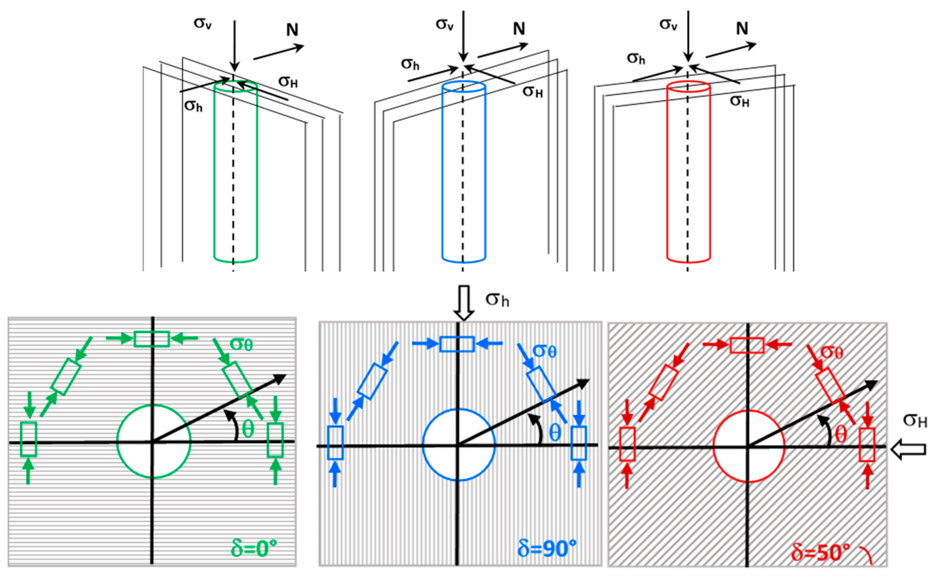
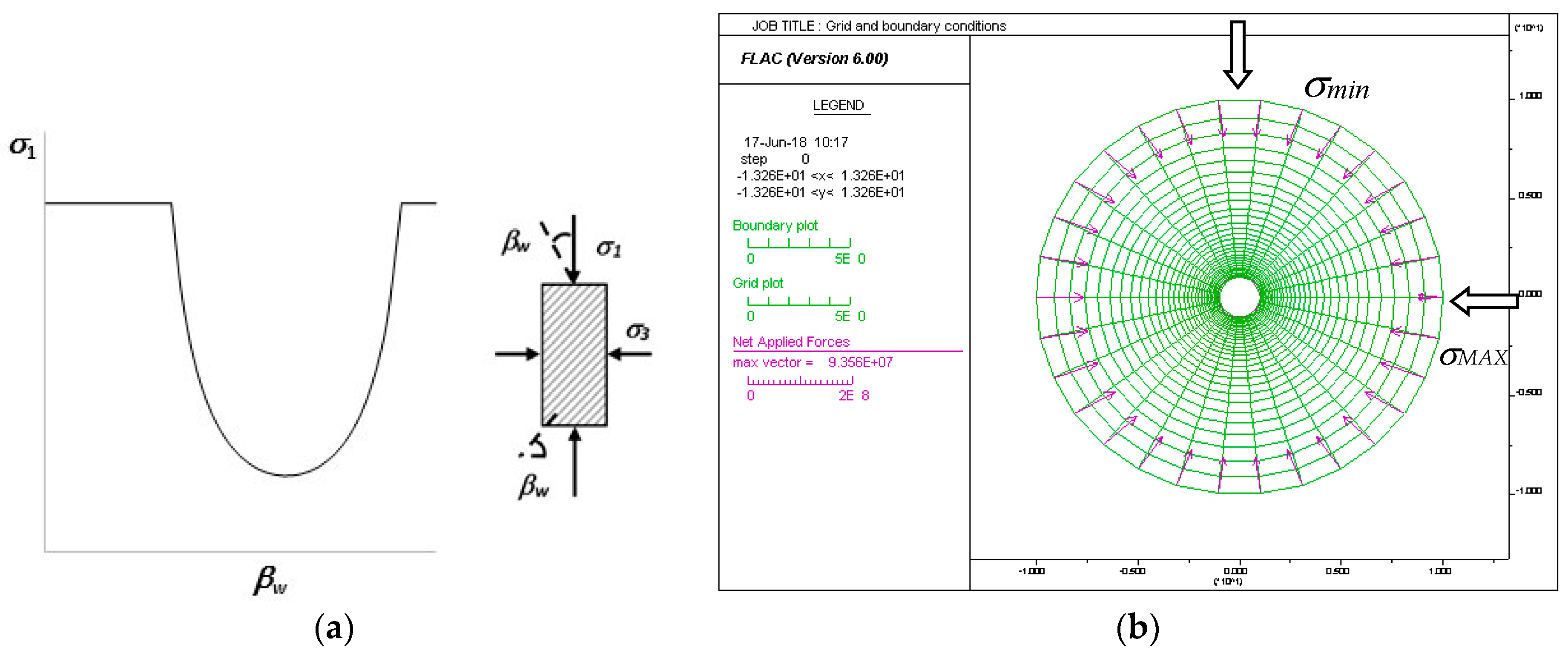
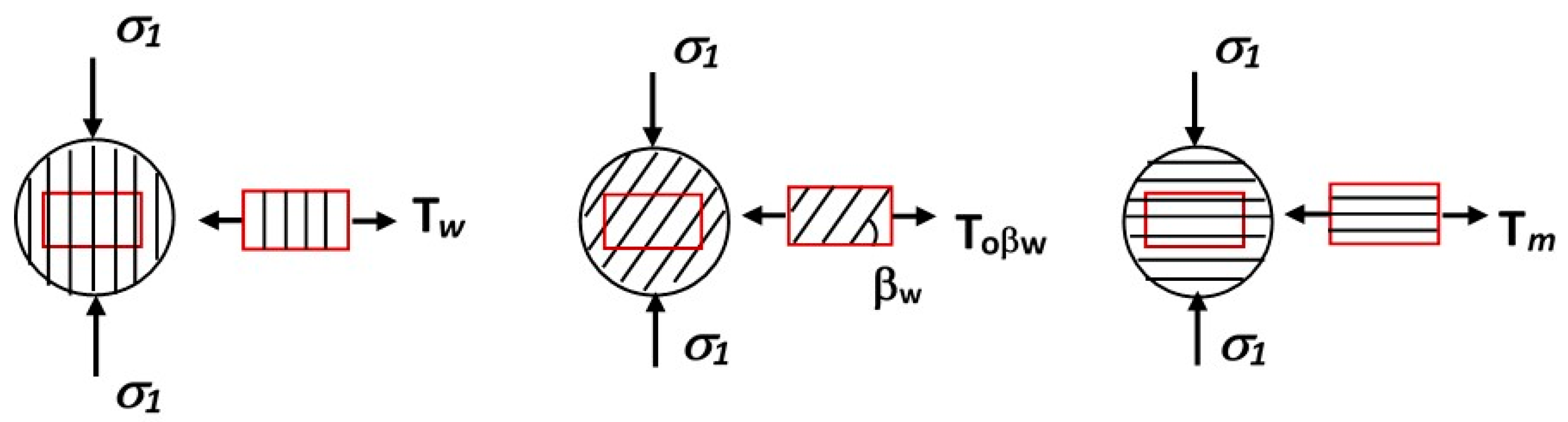
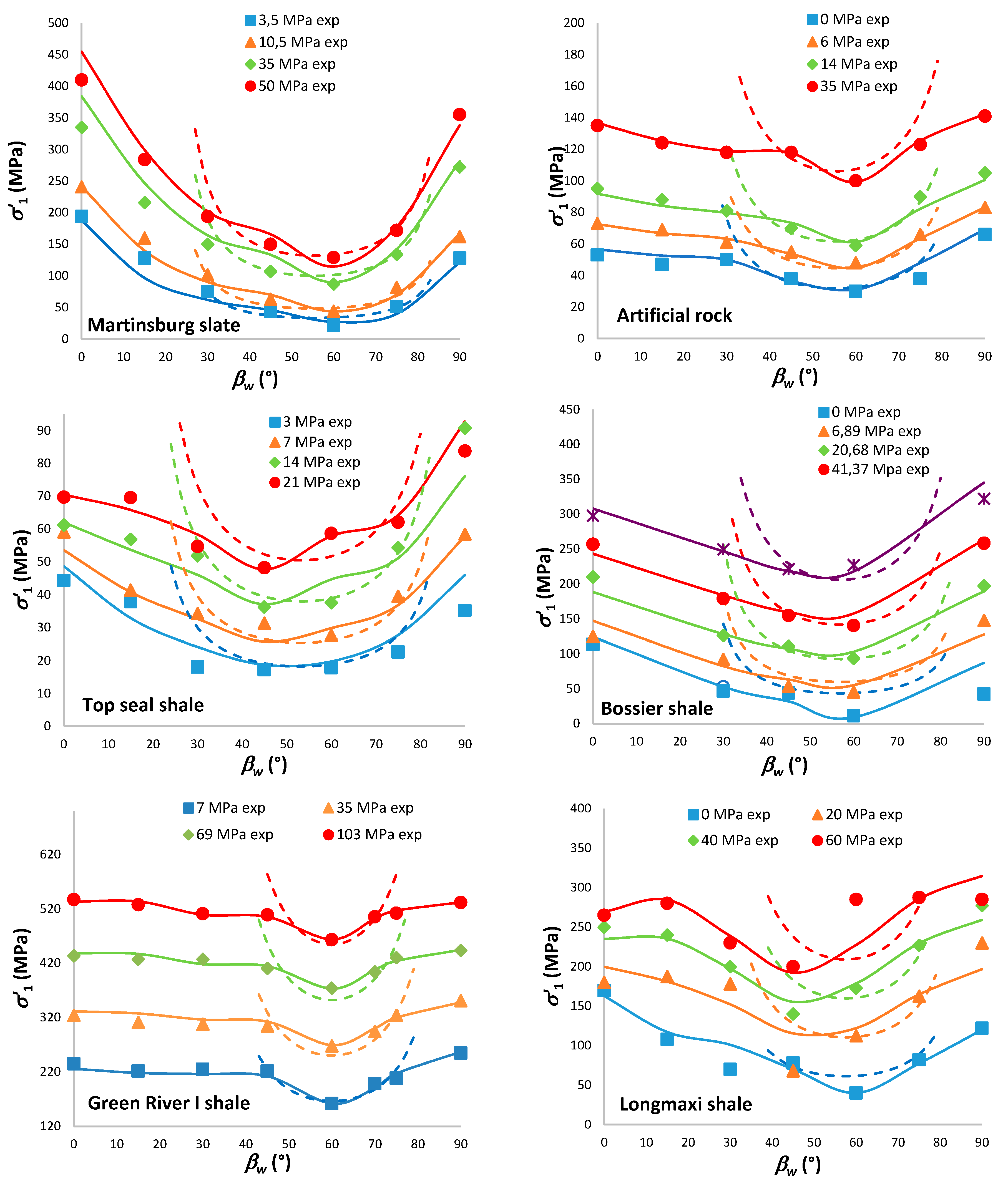
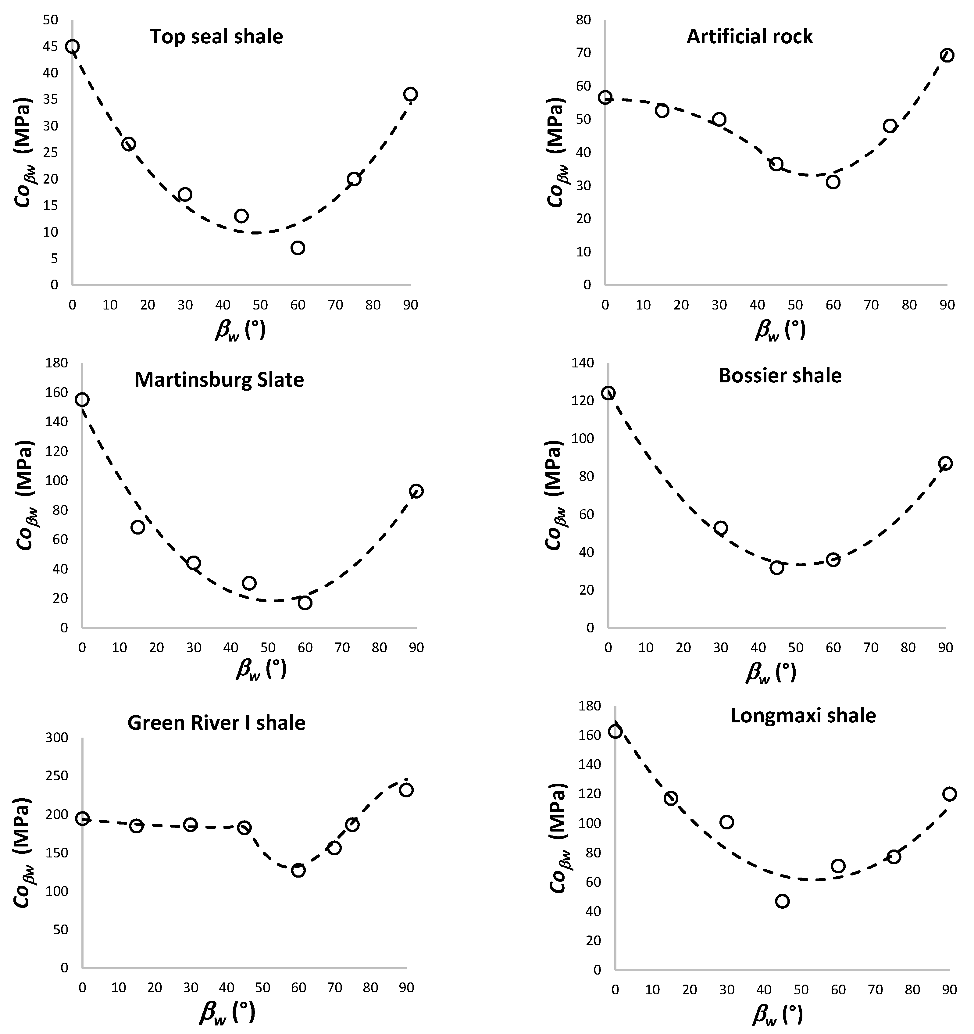
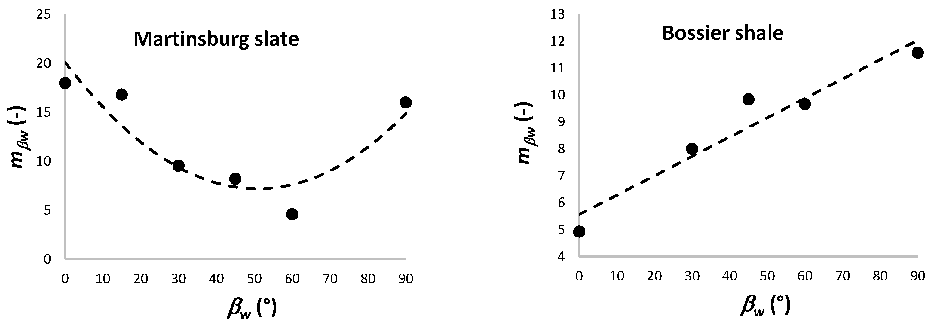
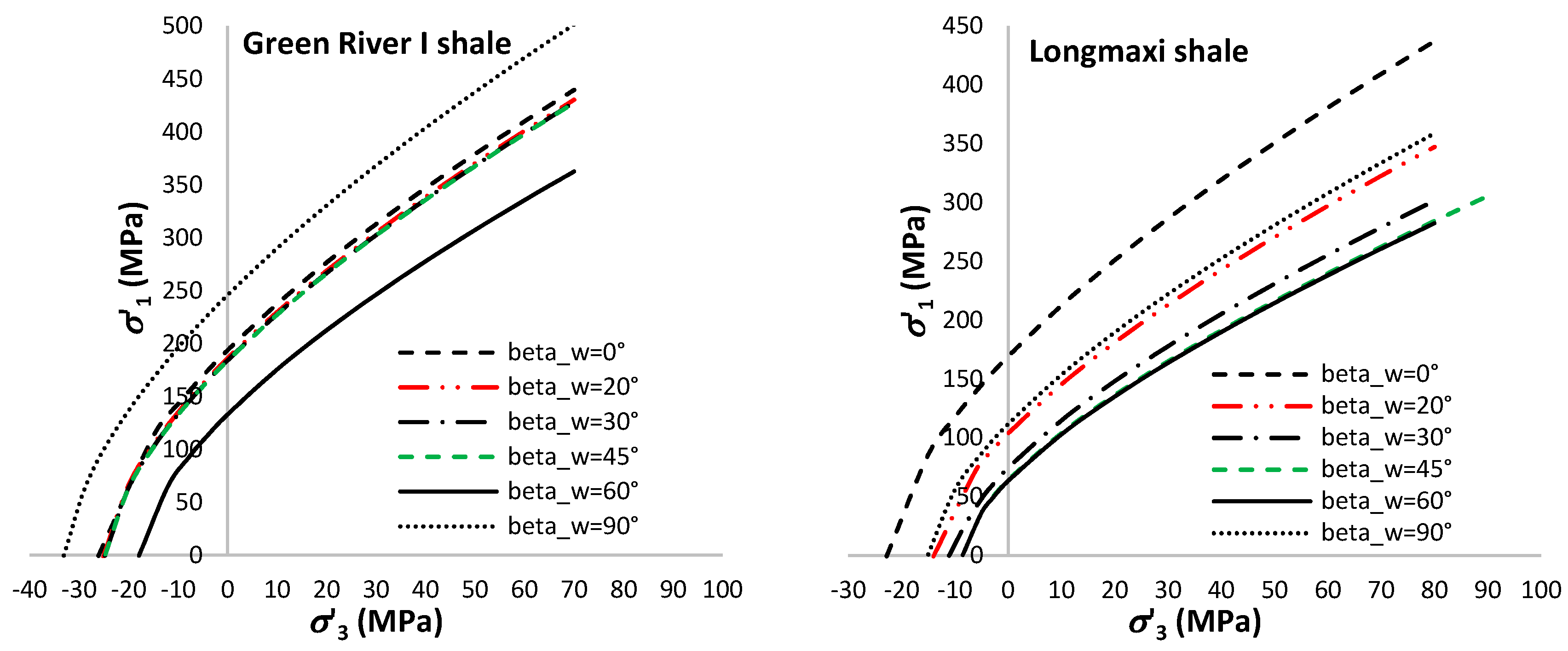
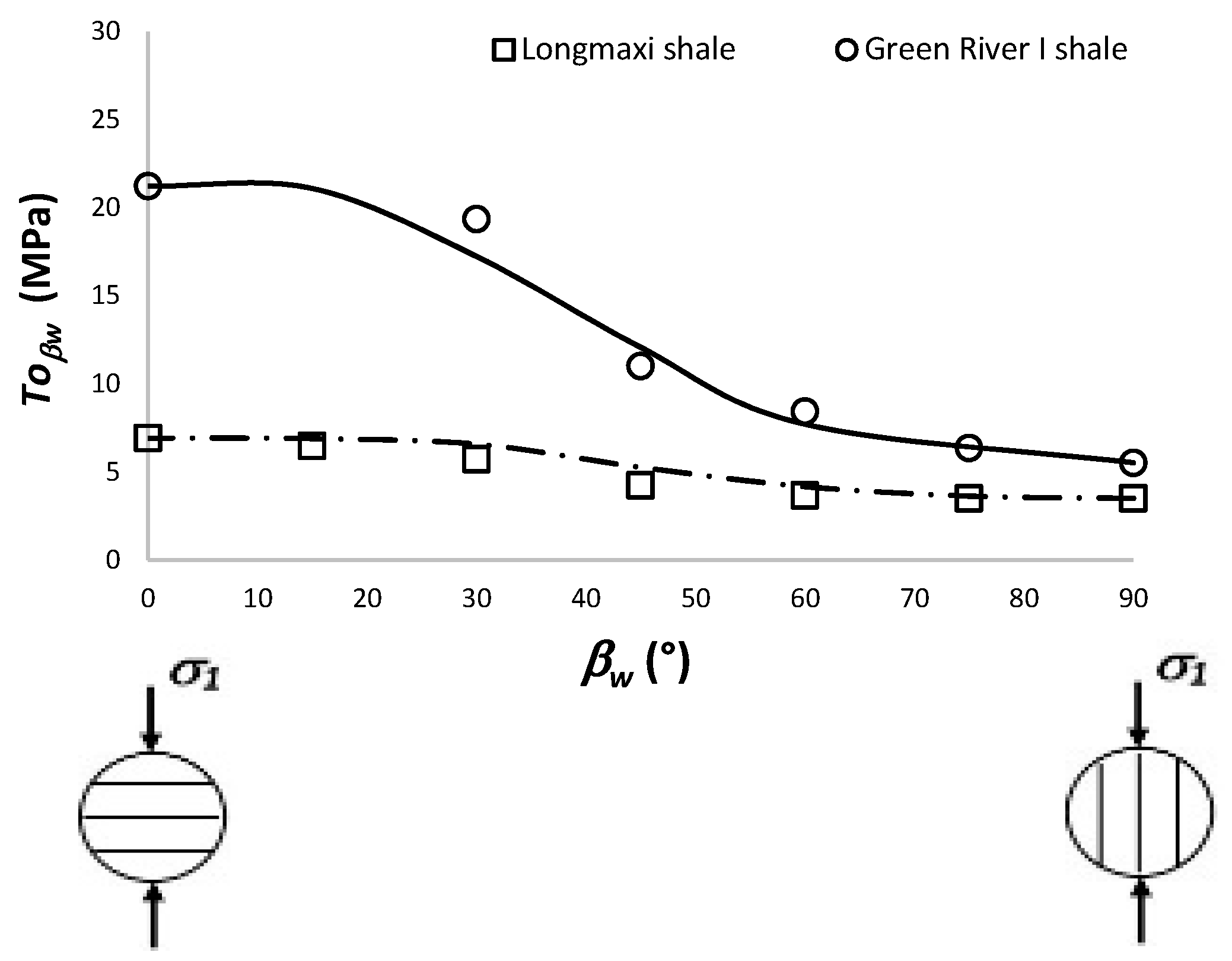
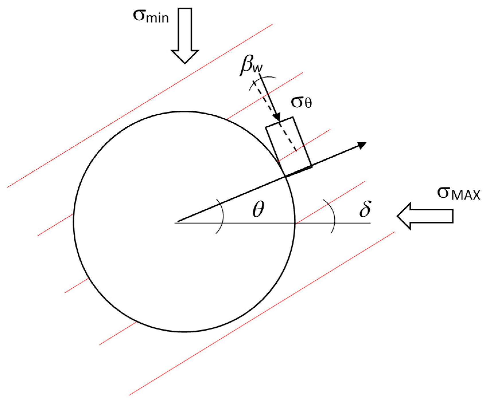
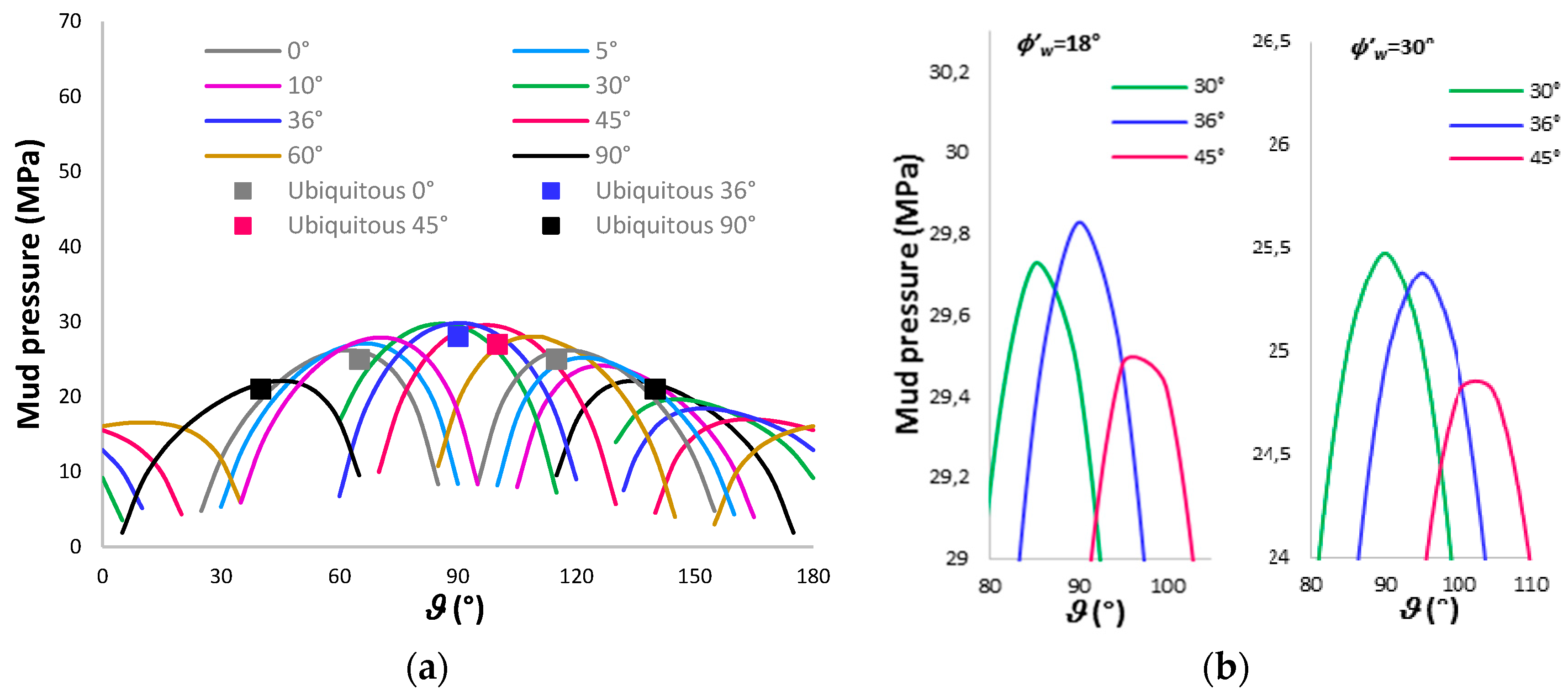
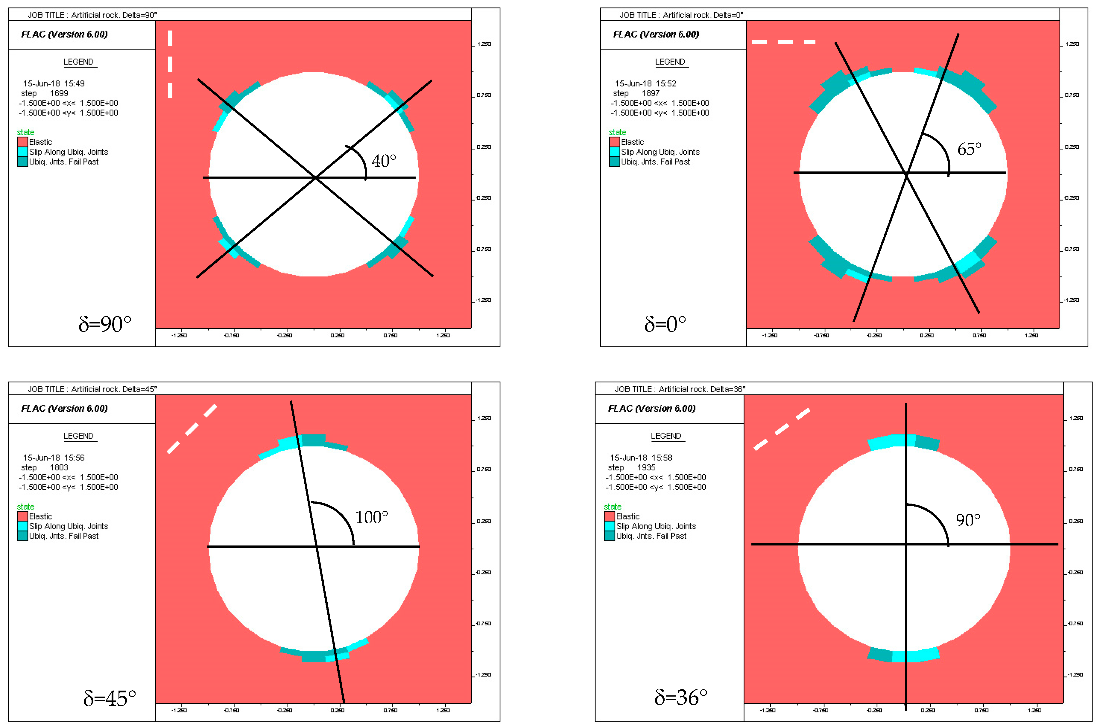
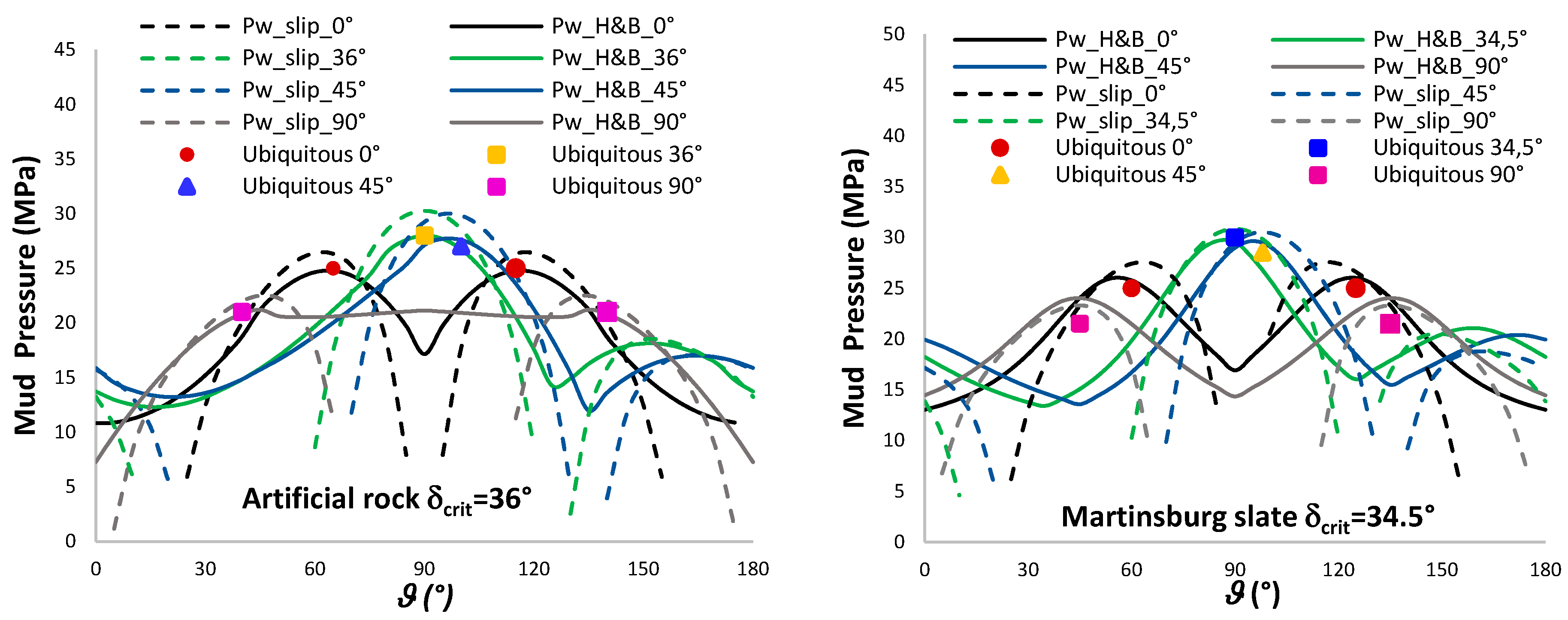
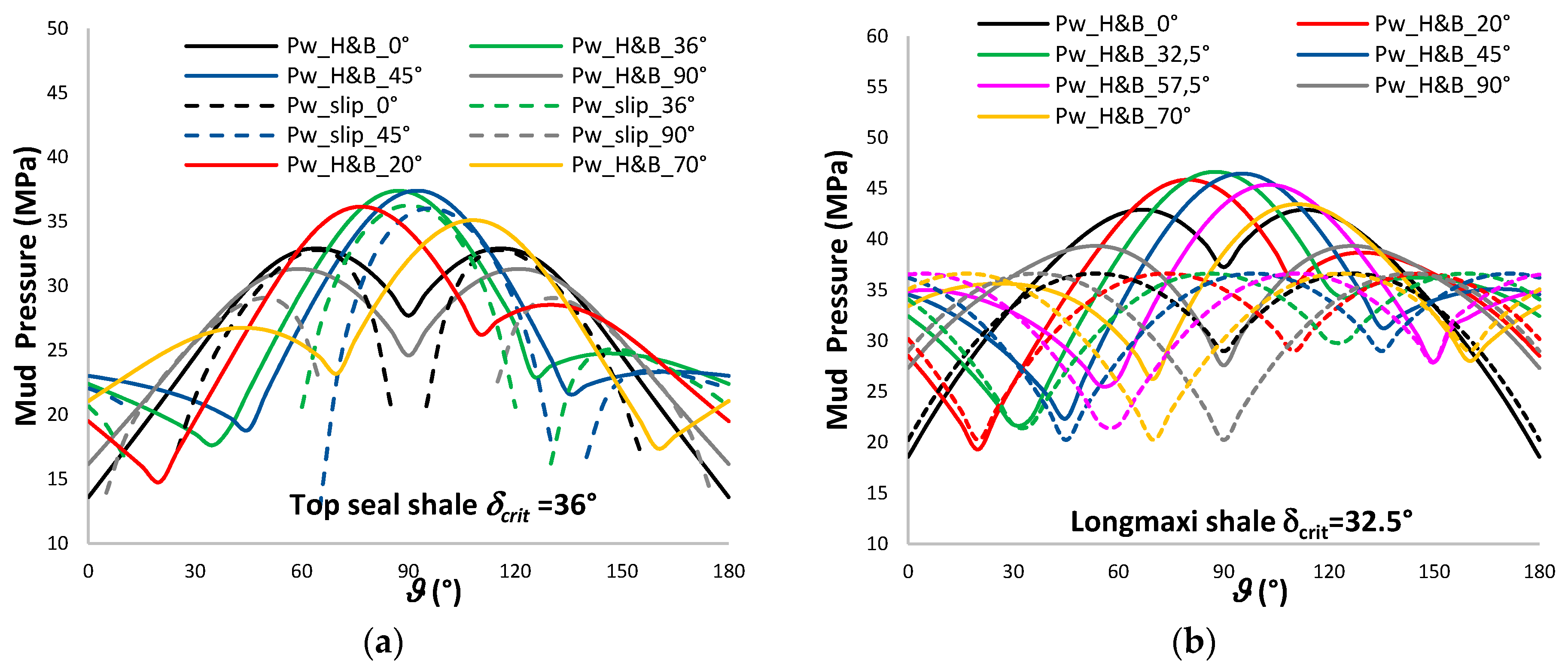
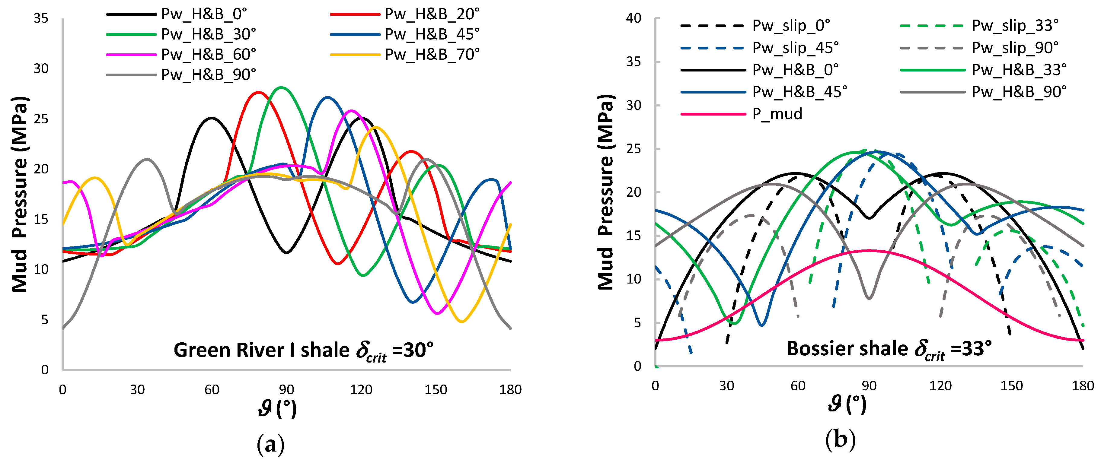
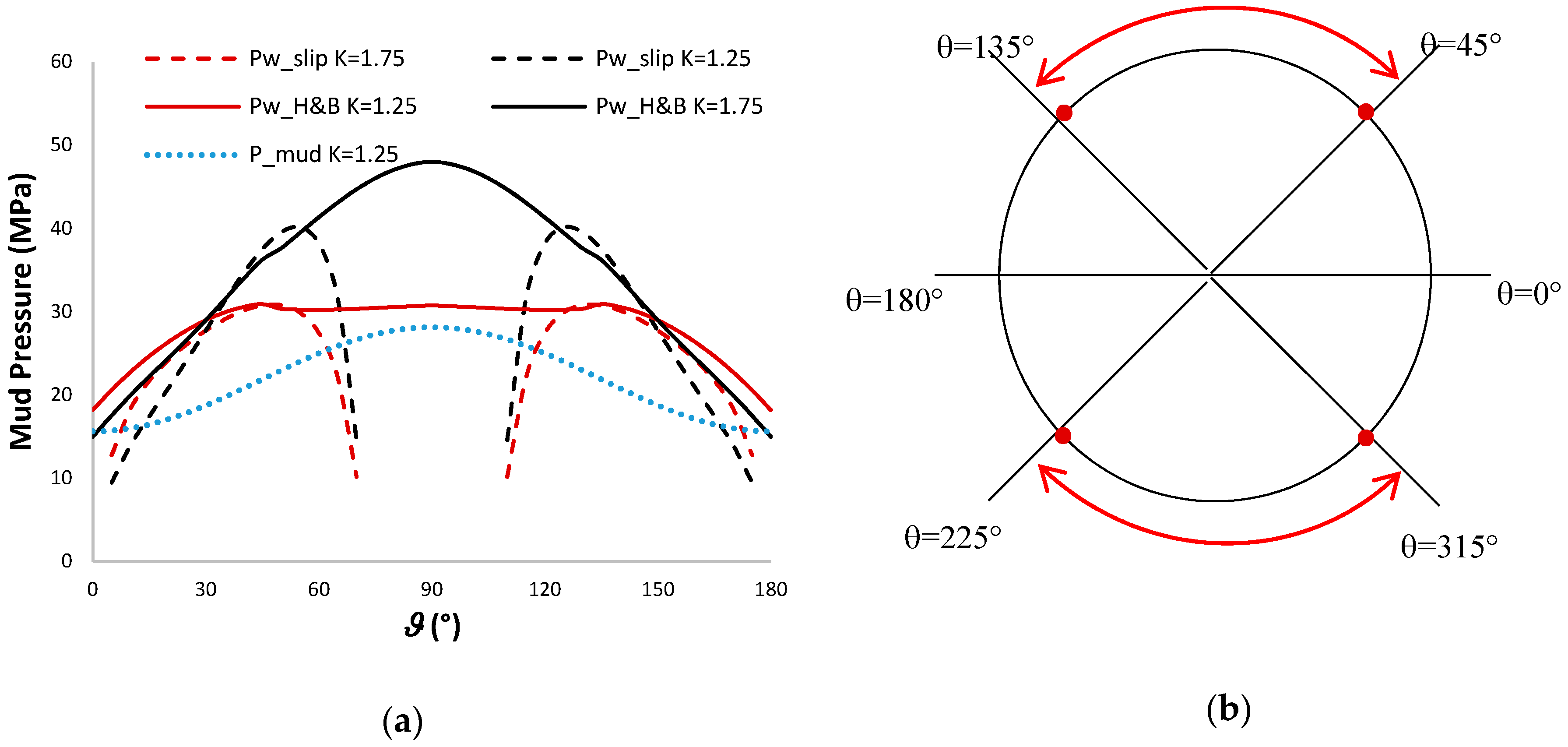
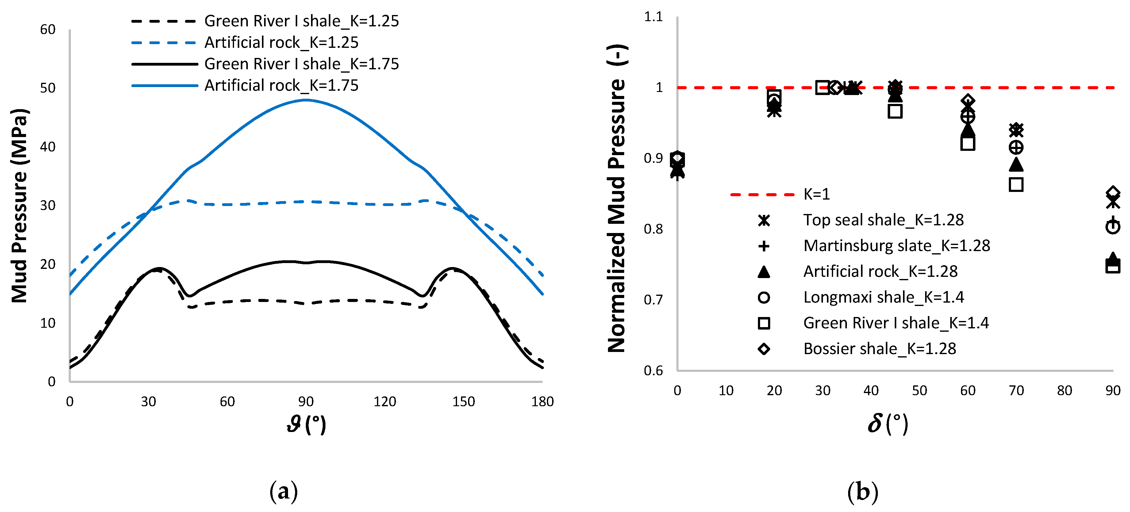
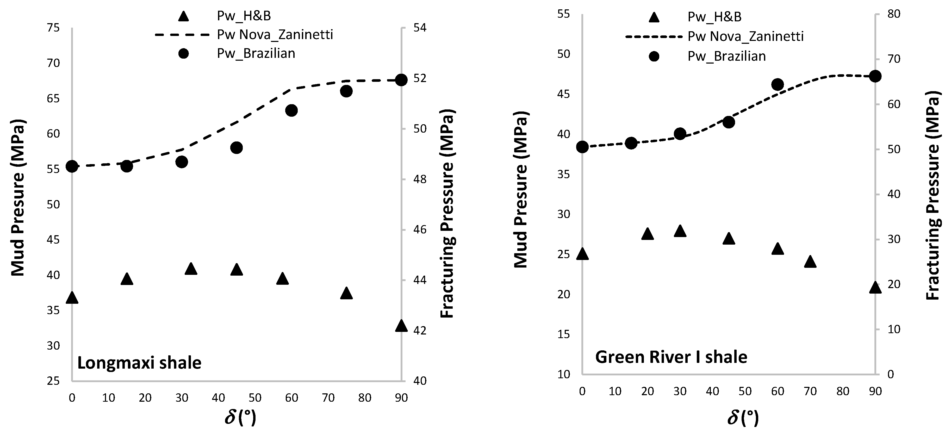
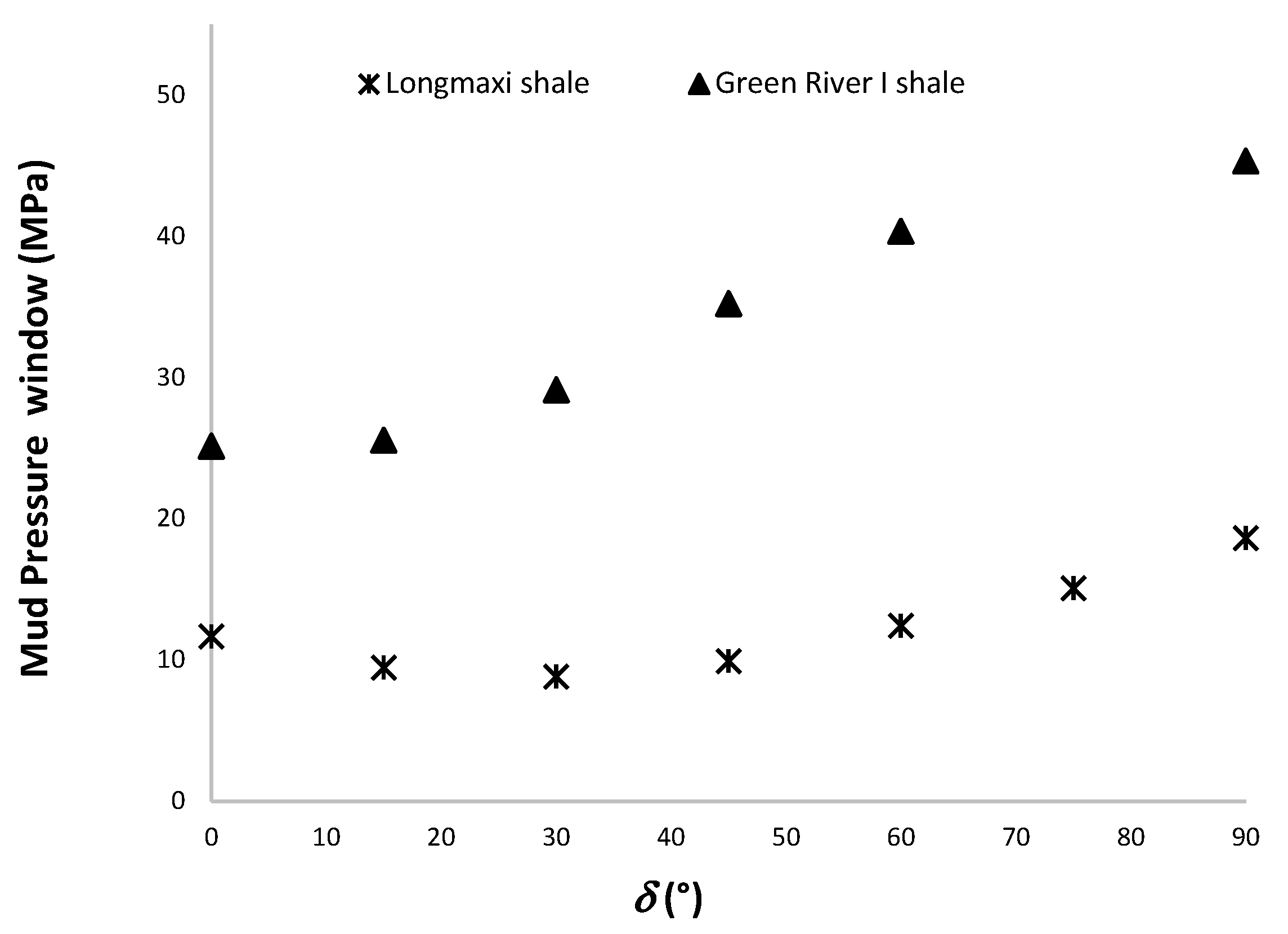
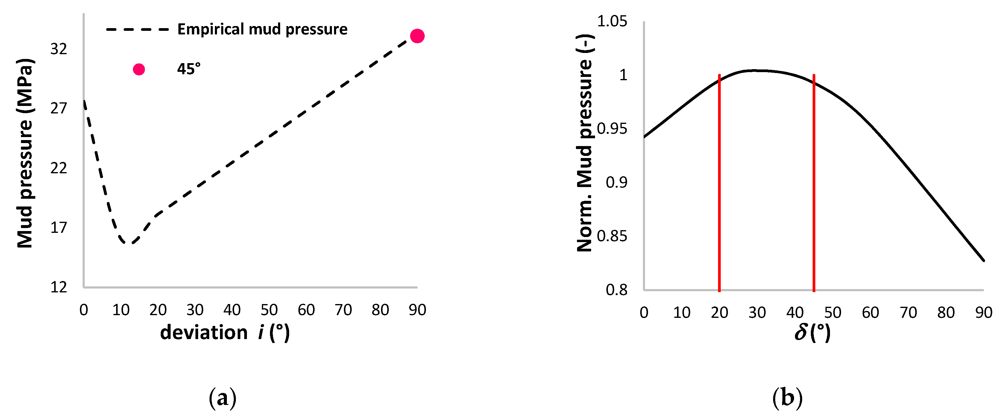
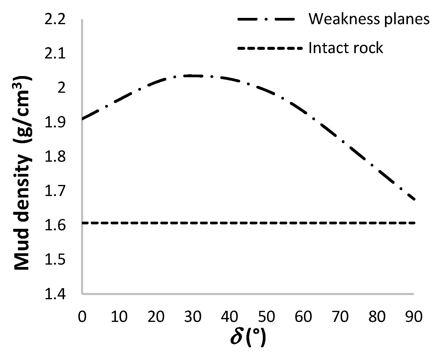
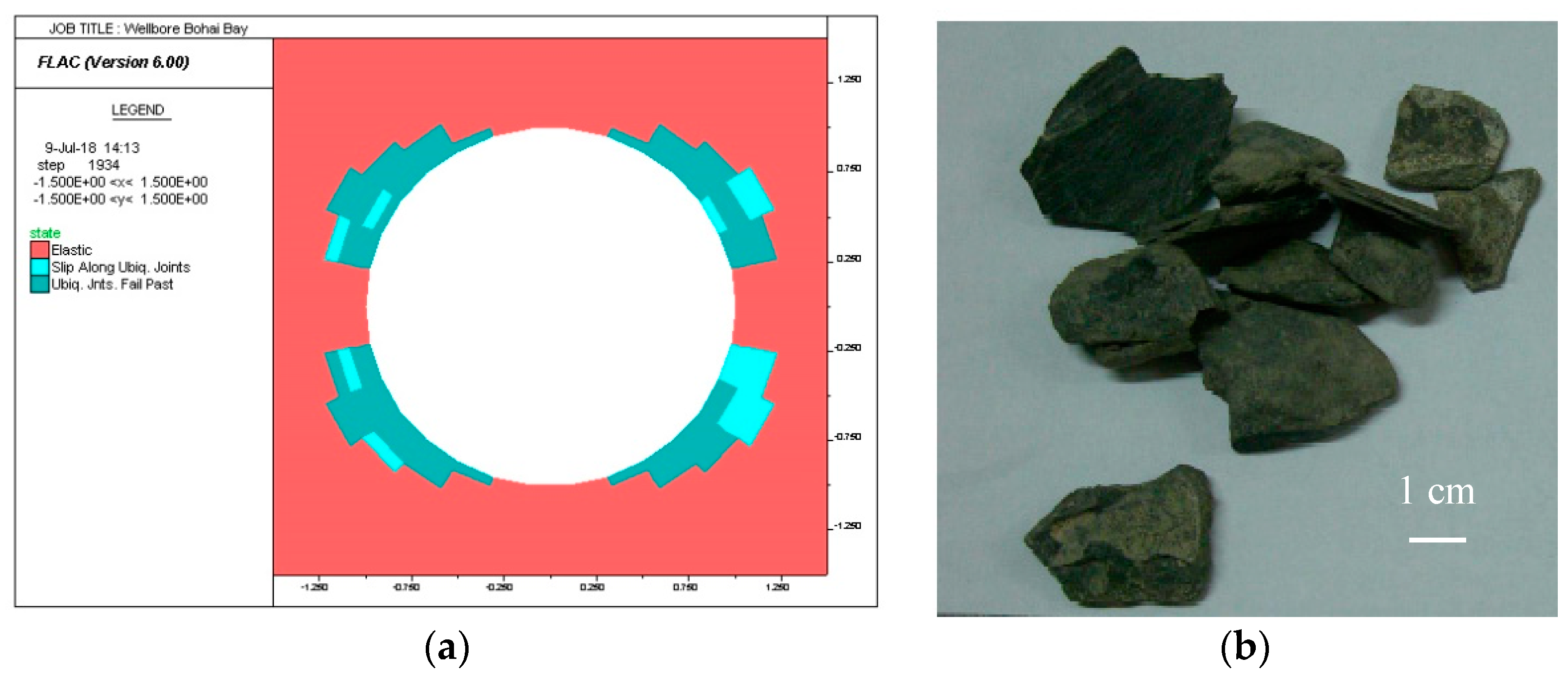
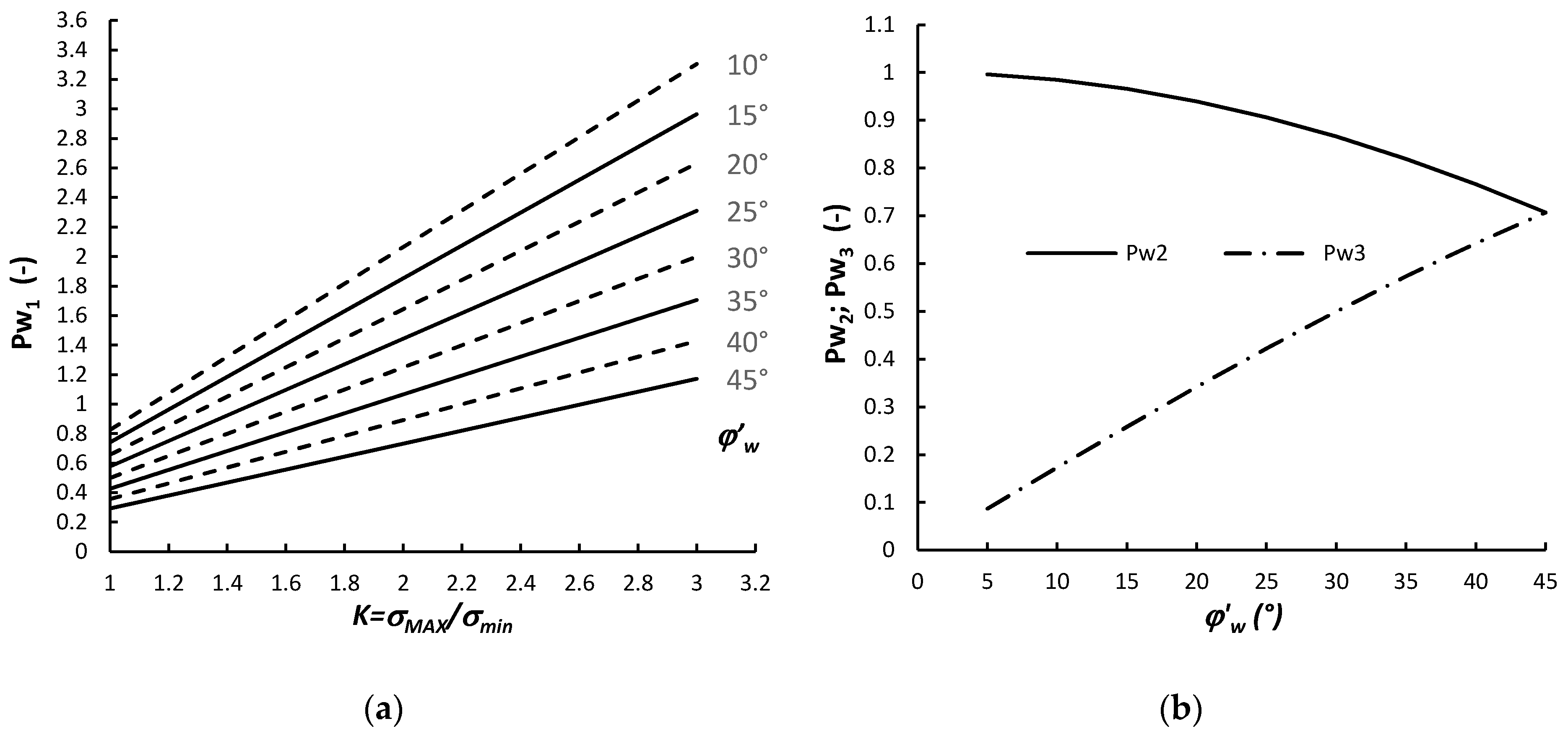
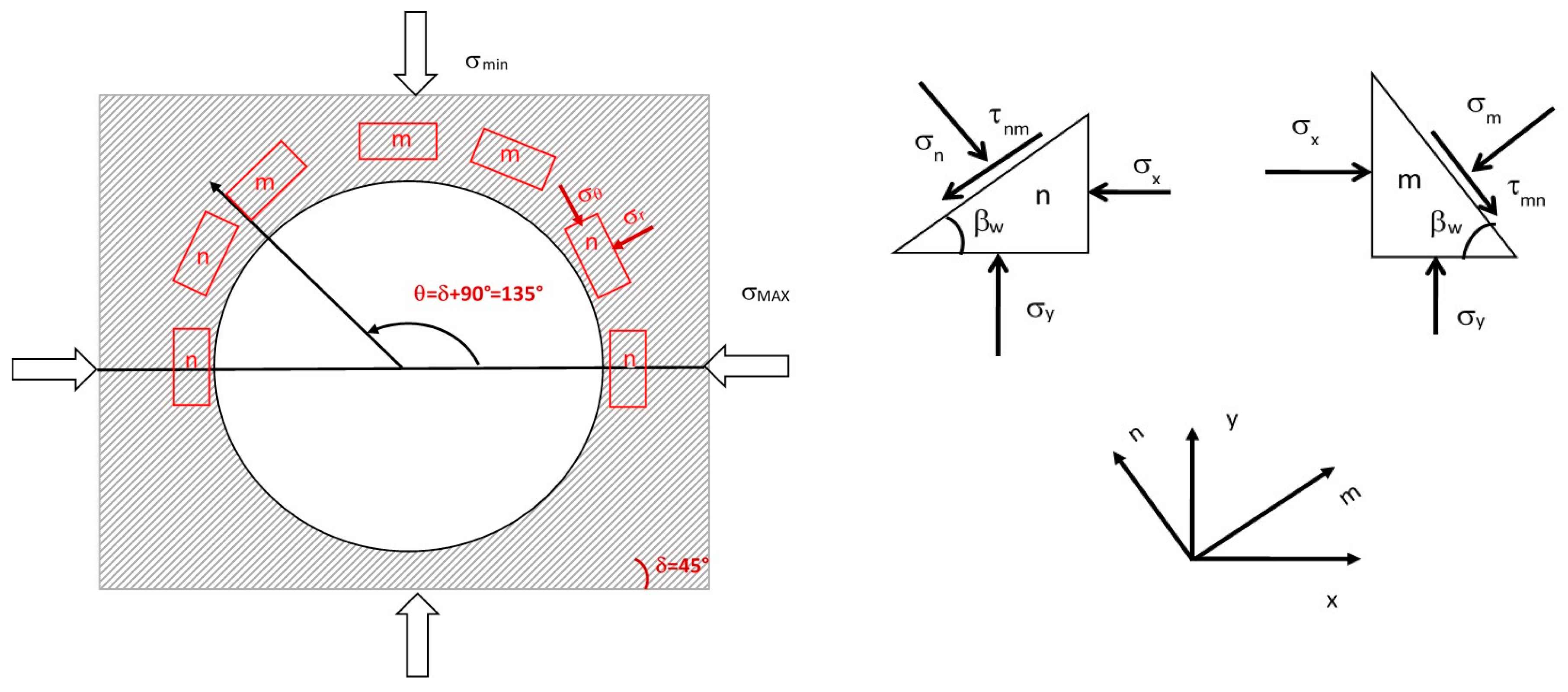
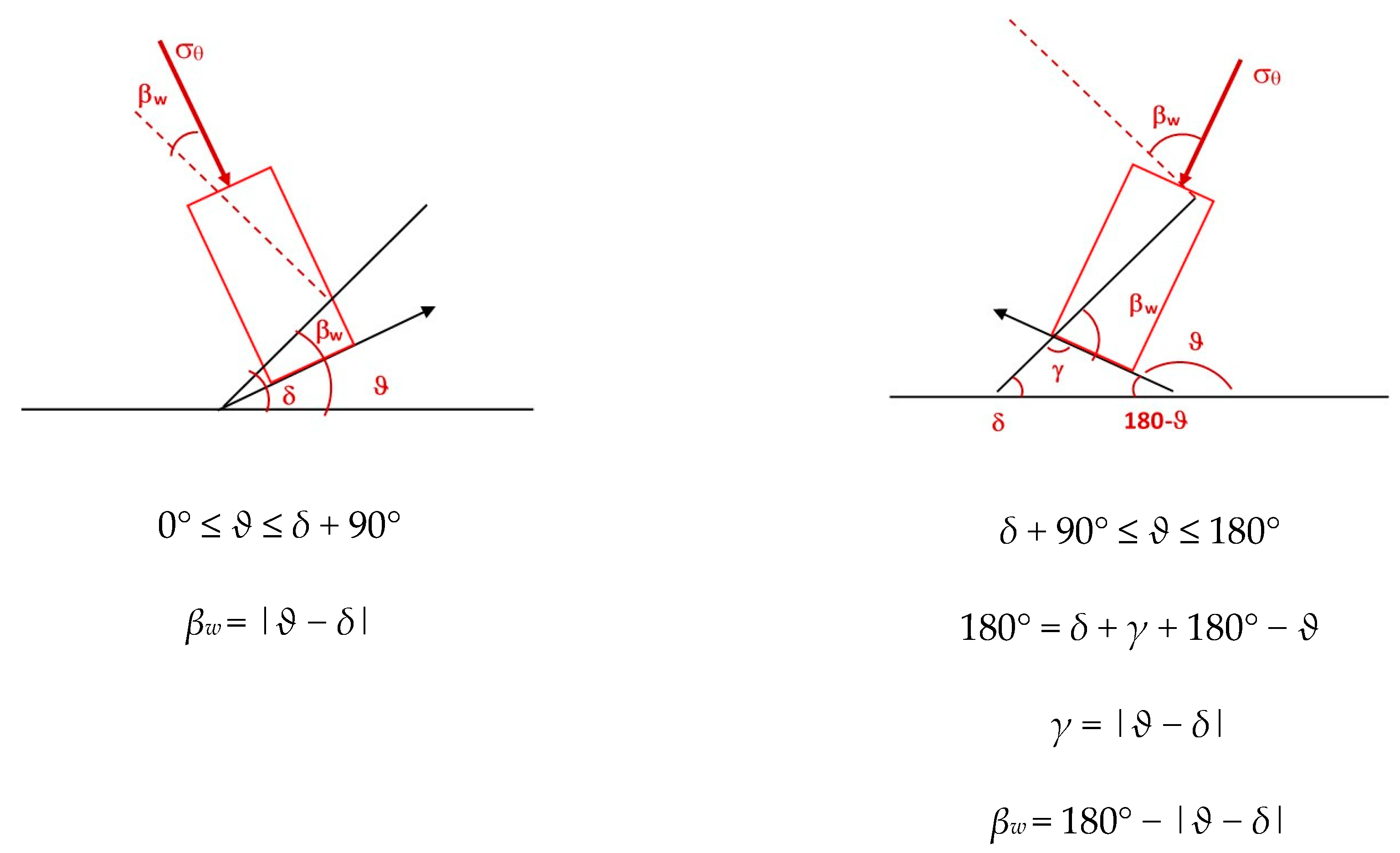
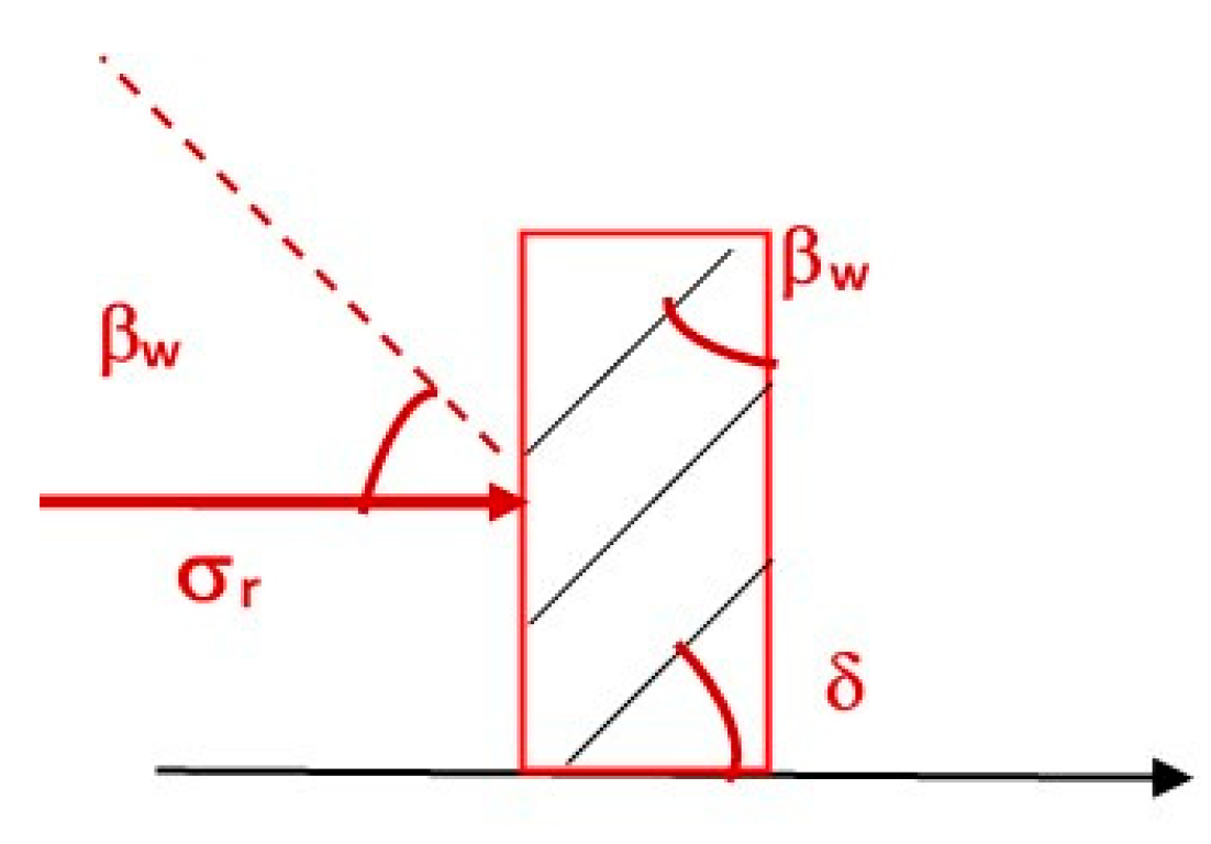
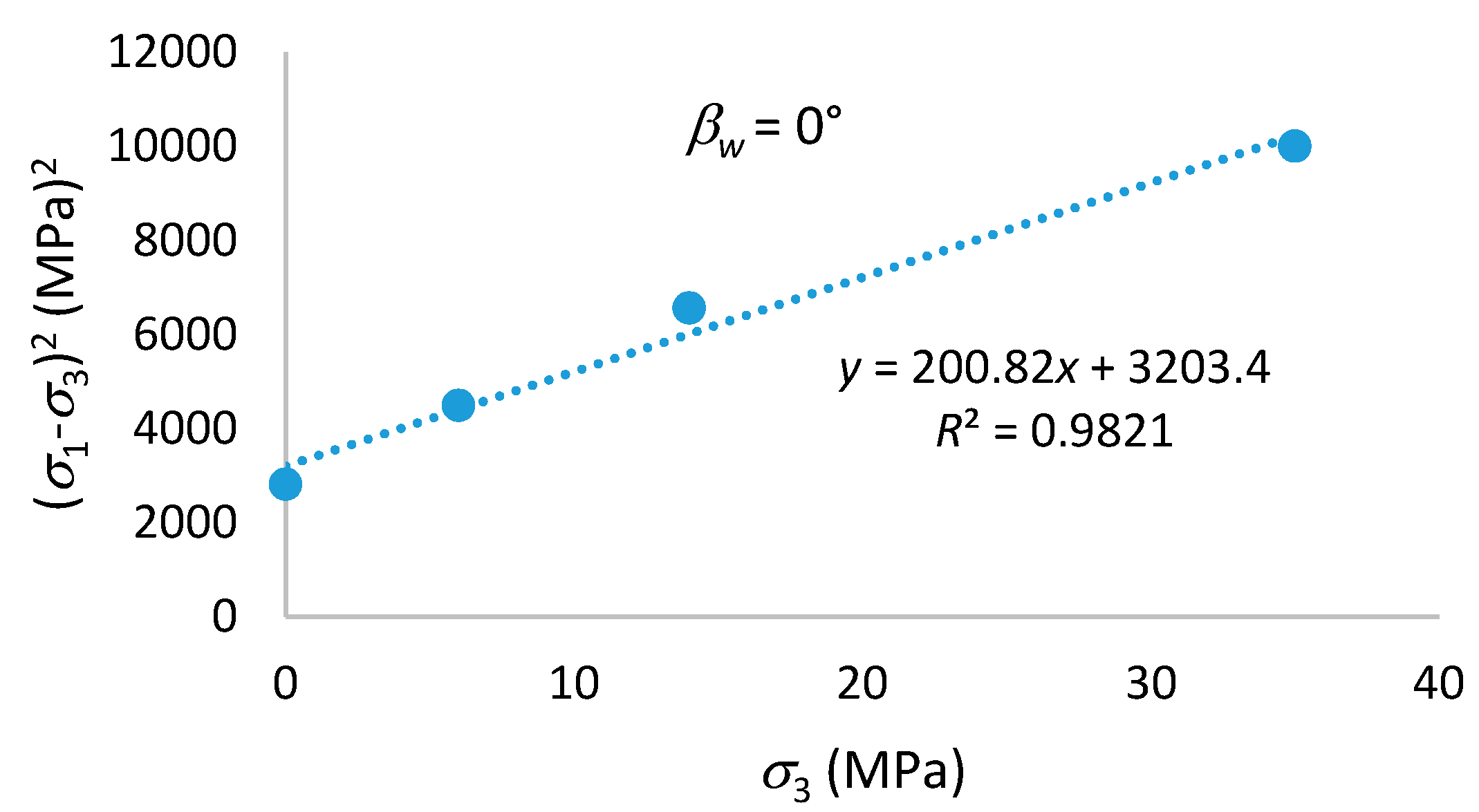
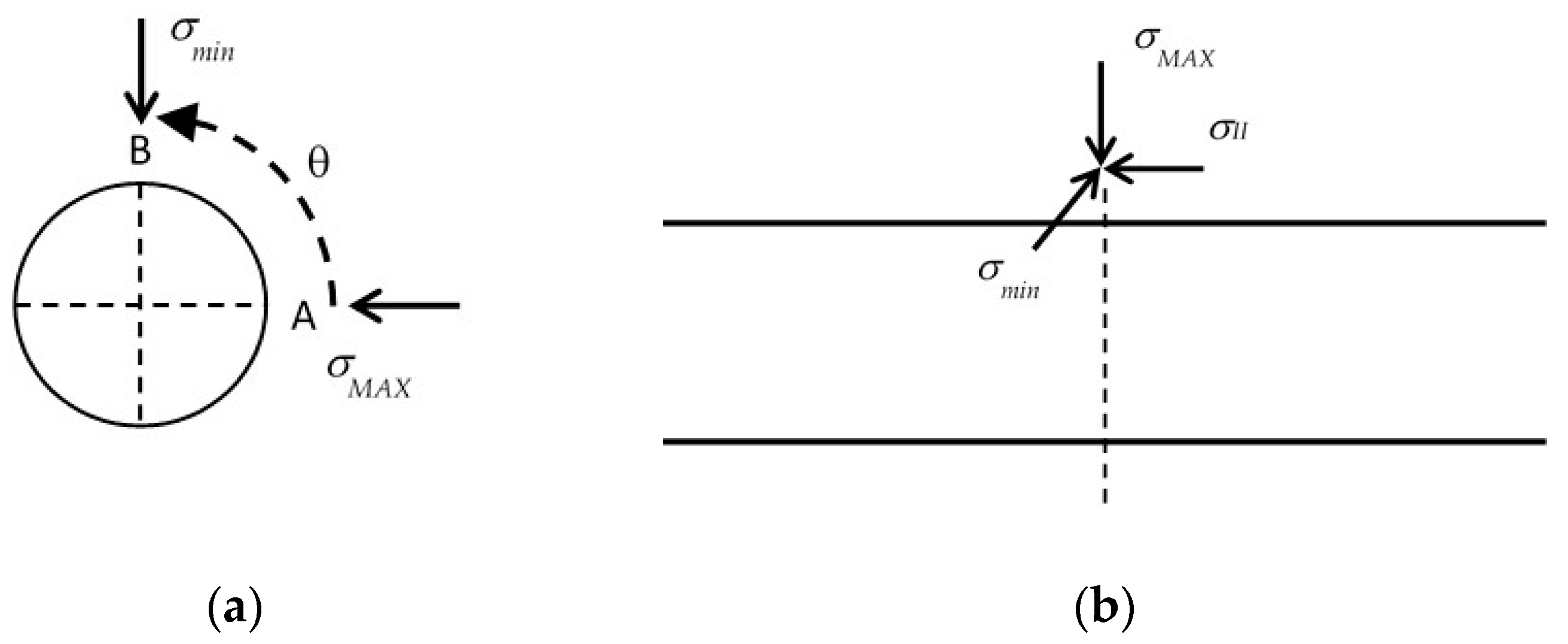
Table 1.
Strength parameters of the weakness planes of the rocks.
| Rock | c’w (MPa) | φ’w (°) |
|---|---|---|
| Artificial rock (*) | 11 | 18 |
| Martinsburg Slate (**) | 9 | 21 |
| Top seal shale (§) | 4.7 | 18 |
| Bossier shale (×) | 14.1 | 24 |
| Green River I shale (#) | 38 | 30 |
| Longmaxi shale (°°) | 19 | 25 |
Table 2.
Instantaneous constants mβw of the Hoek and Brown criterion.
| βw (°) | Artificial Rock | Top Seal Shale | Green River I Shale | Longmaxi Shale |
|---|---|---|---|---|
| 0 | 3.6 | 0.45 | 7.33 | 1.78 |
| 15 | 2.94 | 2.33 | 7.91 | 5.22 |
| 30 | 2.6 | 3.1 | 6.75 | 3.60 |
| 45 | 4.3 | 2 | 6.82 | 5.00 |
| 60 | 2.9 | 9 | 8.67 | 12.00 |
| 75 | 3.5 | 3.5 | 7.08 | 9.68 |
| 90 | 2.78 | 5.1 | 5.45 | 7.00 |
Table 3.
Data and strength criteria used for the calculation of mud pressures for slip and fracturing.
Table 3.
Data and strength criteria used for the calculation of mud pressures for slip and fracturing.
| σMAX (MPa) | σmin (MPa) | Pf (MPa) | Criterion | Rock |
|---|---|---|---|---|
| 45 | 35 | 20 | WPM 1 − UJM 2 − H&B 3 | Artificial rock |
| 45 | 35 | 20 | WPM 1 − UJM 2 − H&B 3 | Martinsburg slate |
| 45 | 35 | 20 | WPM 1 − H&B 3 | Top seal shale |
| 45 | 35 | 20 | H&B 3 | Bossier shale |
| 35 | 35 | 20 | H&B 3 | Bossier shale |
| 50 | 70 | 35 | H&B 3 − N&Z 4 | Longmaxi shale |
| 50 | 70 | 35 | H&B 3 − N&Z 4 | Green River I shale |
1 Weakness plane model; 2 Ubiquitous Joint Model; 3 Hoek and Brown criterion; 4 Nova and Zaninetti criterion.
Table 4.
Data used for the calculation of mud pressures at the Pedernales Field, Venezuela [5].
Table 4.
Data used for the calculation of mud pressures at the Pedernales Field, Venezuela [5].
| σv (MPa) | σH (MPa) | σh (MPa) | Pf (MPa) | Depth (m) | α-σH1 (°) | α-WP 2 (°) | Ψ-WP 3 (°) | c’w (MPa) | φ’w (°) | Co (MPa) | φ’ (°) |
|---|---|---|---|---|---|---|---|---|---|---|---|
| 37.2 | 45.5 | 35 | 17.7 | 1676 | 315 | 315 | 45 | 2.1 | 26.6 | 28.96 | 31 |
1 Dip direction of the maximum horizontal stress; 2 Dip direction of the weakness planes; 3 Dip of the weakness planes.
Table 5.
Data used for the calculation of mud pressures in a horizontal wellbore drilled in Bohai Bay (China) [8].
Table 5.
Data used for the calculation of mud pressures in a horizontal wellbore drilled in Bohai Bay (China) [8].
| σv (MPa) | σH (MPa) | σh (MPa) | Pf (MPa) | Depth (m) | c’w (MPa) | φ’w (°) |
|---|---|---|---|---|---|---|
| 30 | 27.5 | 25 | 15 | 1540 | 2.75 | 20 |
© 2018 by the authors. Licensee MDPI, Basel, Switzerland. This article is an open access article distributed under the terms and conditions of the Creative Commons Attribution (CC BY) license (http://creativecommons.org/licenses/by/4.0/).
Share and Cite
MDPI and ACS Style
Deangeli, C.; Omwanghe, O.O. Prediction of Mud Pressures for the Stability of Wellbores Drilled in Transversely Isotropic Rocks. Energies 2018, 11, 1944. https://doi.org/10.3390/en11081944
AMA Style
Deangeli C, Omwanghe OO. Prediction of Mud Pressures for the Stability of Wellbores Drilled in Transversely Isotropic Rocks. Energies. 2018; 11(8):1944. https://doi.org/10.3390/en11081944
Chicago/Turabian StyleDeangeli, Chiara, and Omoruyi Omoman Omwanghe. 2018. "Prediction of Mud Pressures for the Stability of Wellbores Drilled in Transversely Isotropic Rocks" Energies 11, no. 8: 1944. https://doi.org/10.3390/en11081944
Note that from the first issue of 2016, this journal uses article numbers instead of page numbers. See further details here.