Inventory of Glaciers in the Shaksgam Valley of the Chinese Karakoram Mountains, 1970–2014

 ,
,  , ,
, ,
Abstract
:1. Introduction
2. Study Area and Datasets
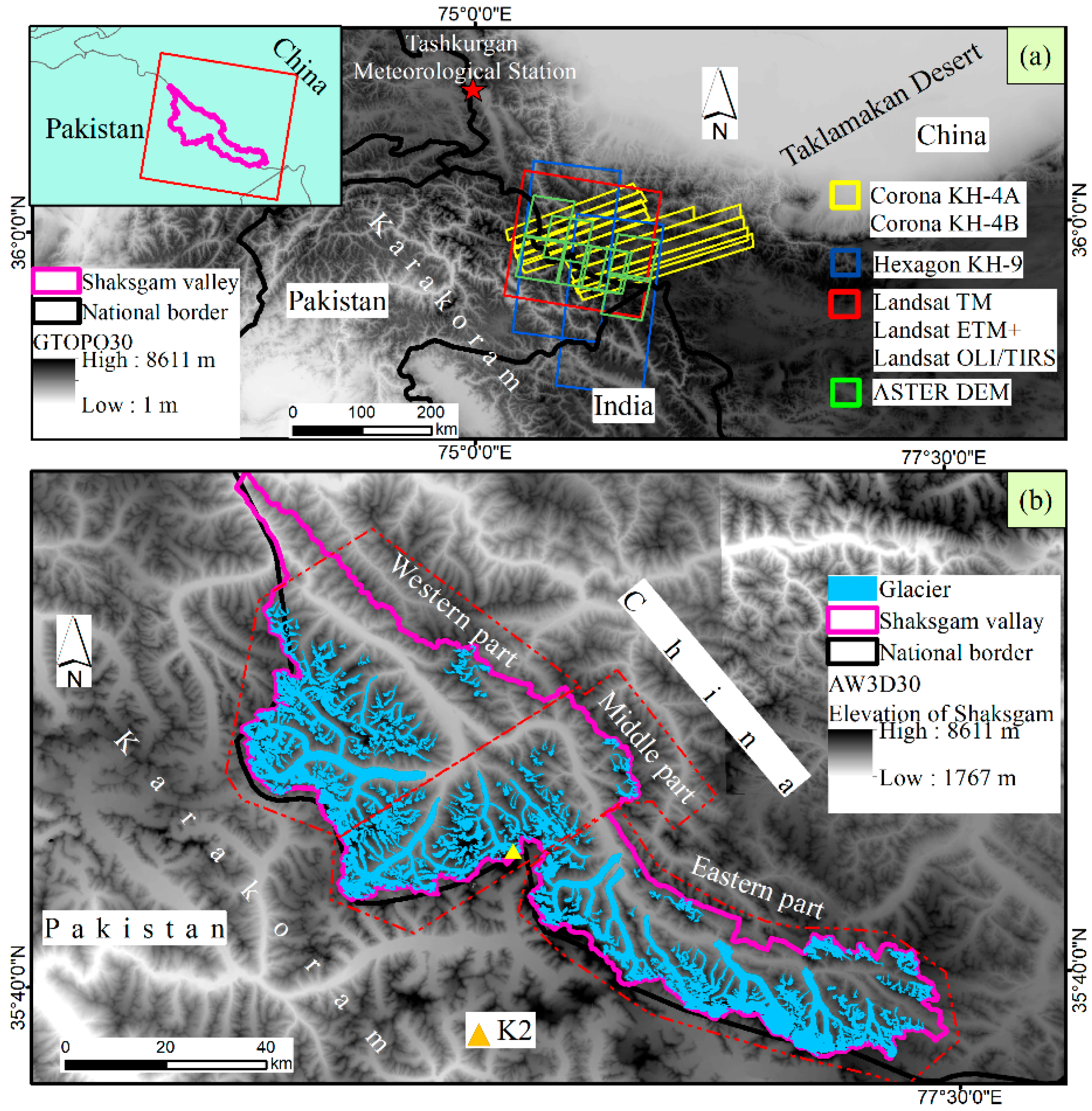
2.1. Study Area
2.2. Datasets
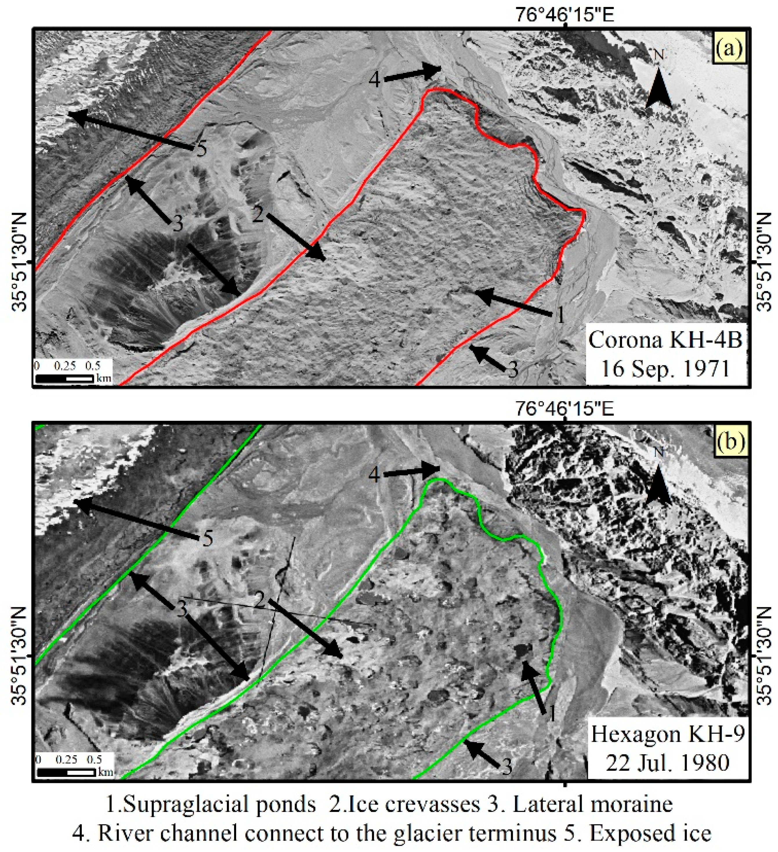
2.2.1. Corona KH-4A/B
2.2.2. Hexagon KH-9
2.2.3. Landsat Series Scenes, ASTER and DEMs
2.2.4. DEM Data Used for Extracting Glacier Topographic Parameters
2.2.5. Climate Data
2.2.6. Validation Datasets
2.2.7. Source of Datasets
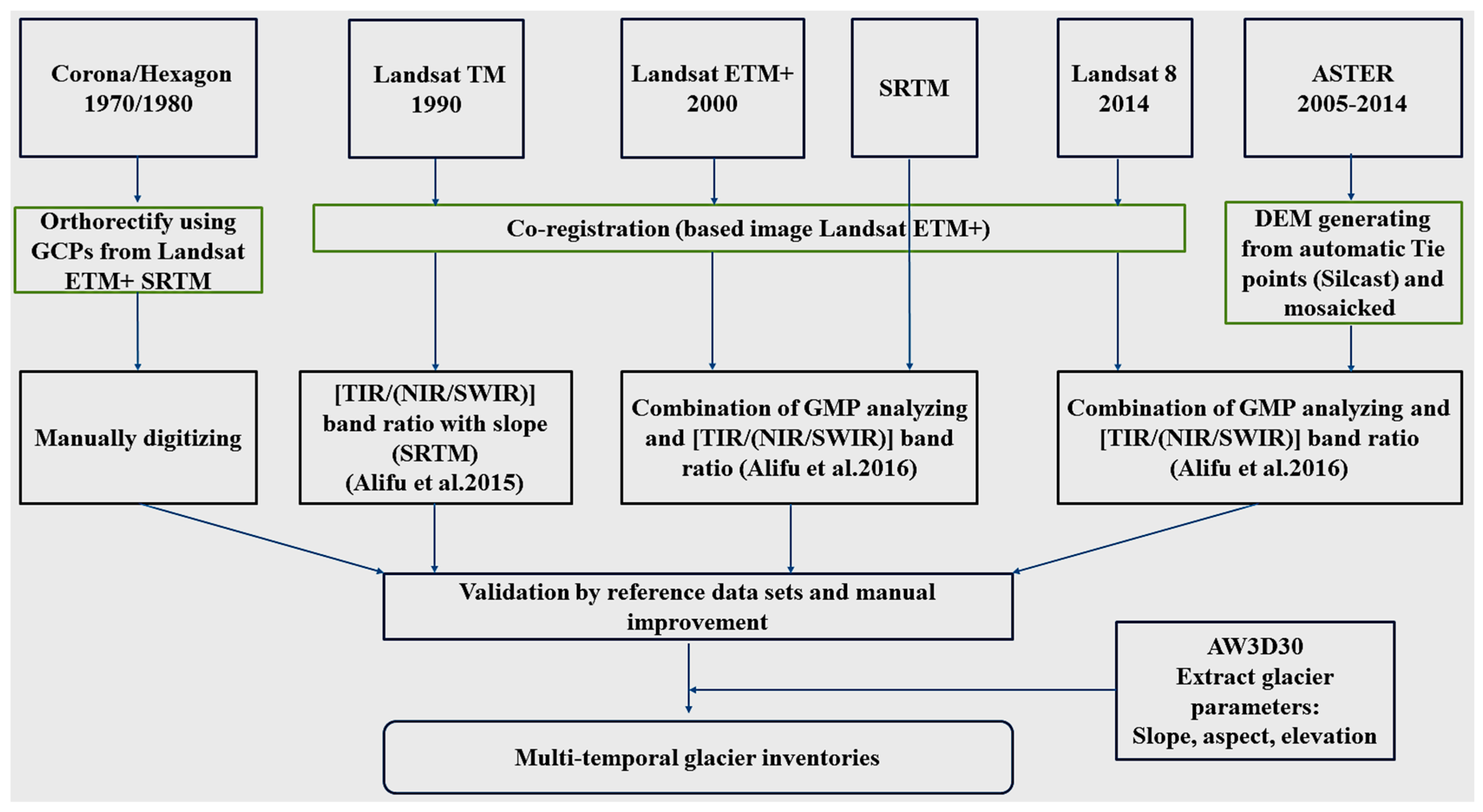
3. Method for Generation of Multi-Temporal Glacier Inventories
3.1. Glacier Inventory 1970/1980
3.1.1. Orthorectification of Corona Images
3.1.2. Orthorectification of Hexagon Images
3.1.3. Manual Delineation of Glaciers Based on the Corona and Hexagon Images
3.2. Glacier Inventory 1990
3.3. Glacier Inventory 2000
3.4. Glacier Inventory 2014
3.5. Complete Glacier Inventory
4. Accuracy Assessment and Error Estimation
5. Results
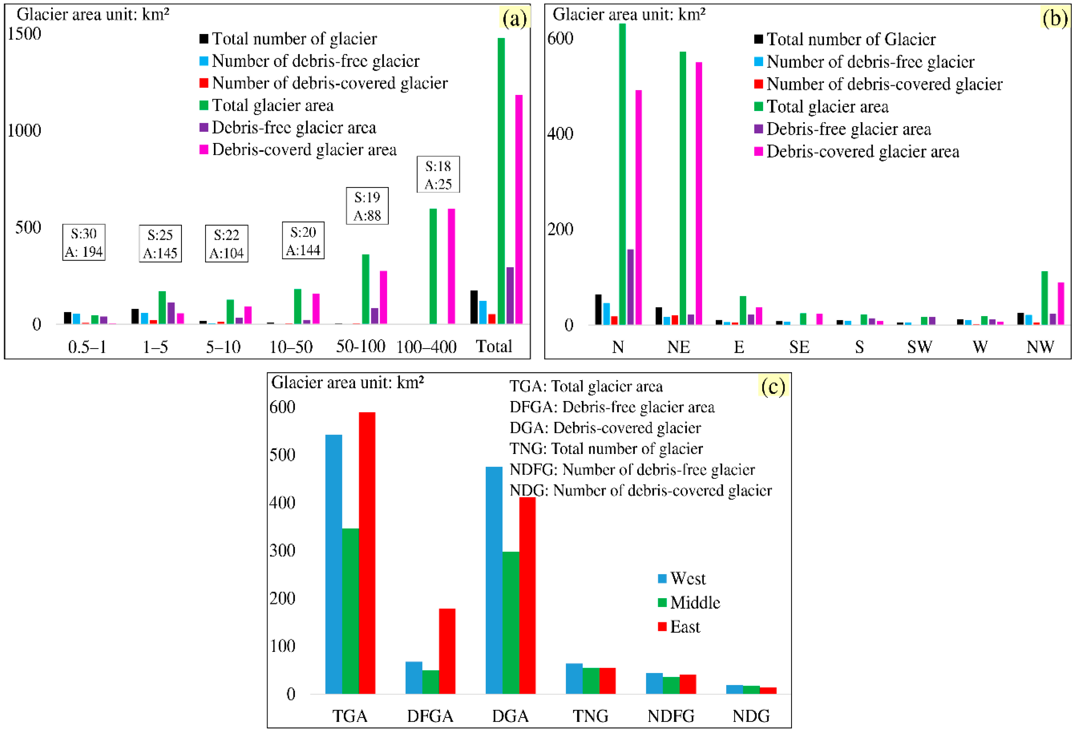
5.1. Updated Glacier (2014) Inventory and Glacier Characteristics
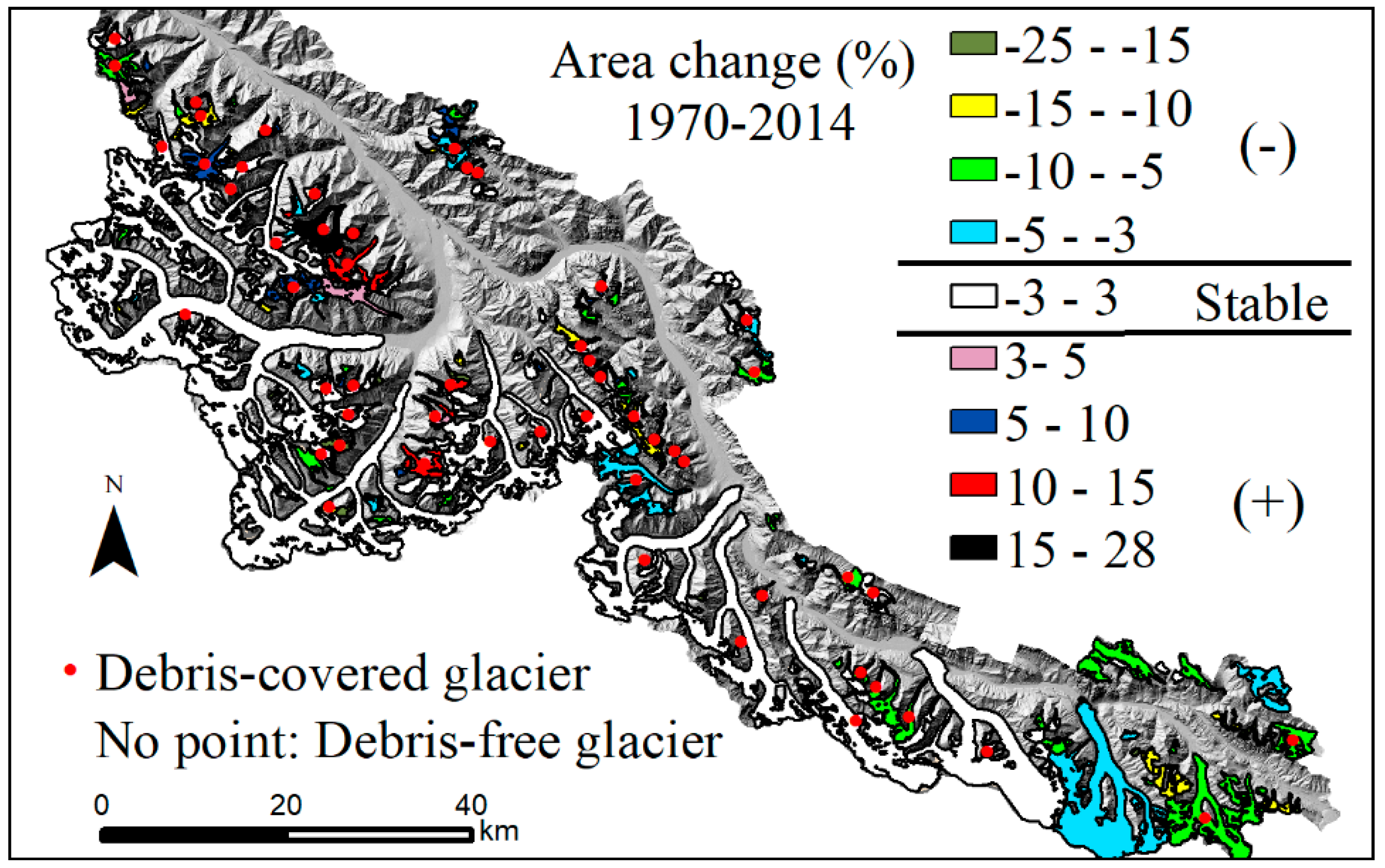
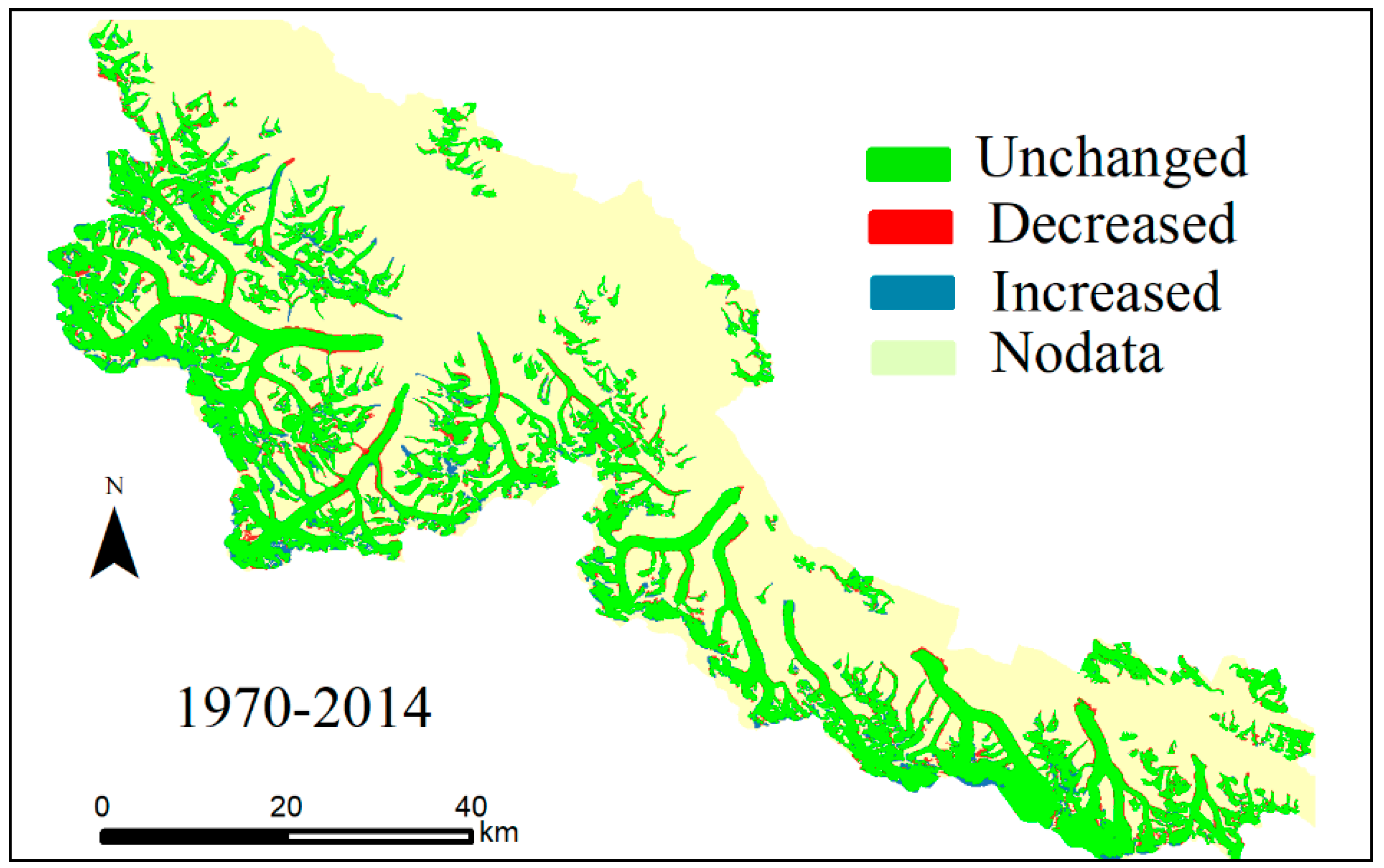
5.2. Glacier Area Change During Four Decades (1970–2014)
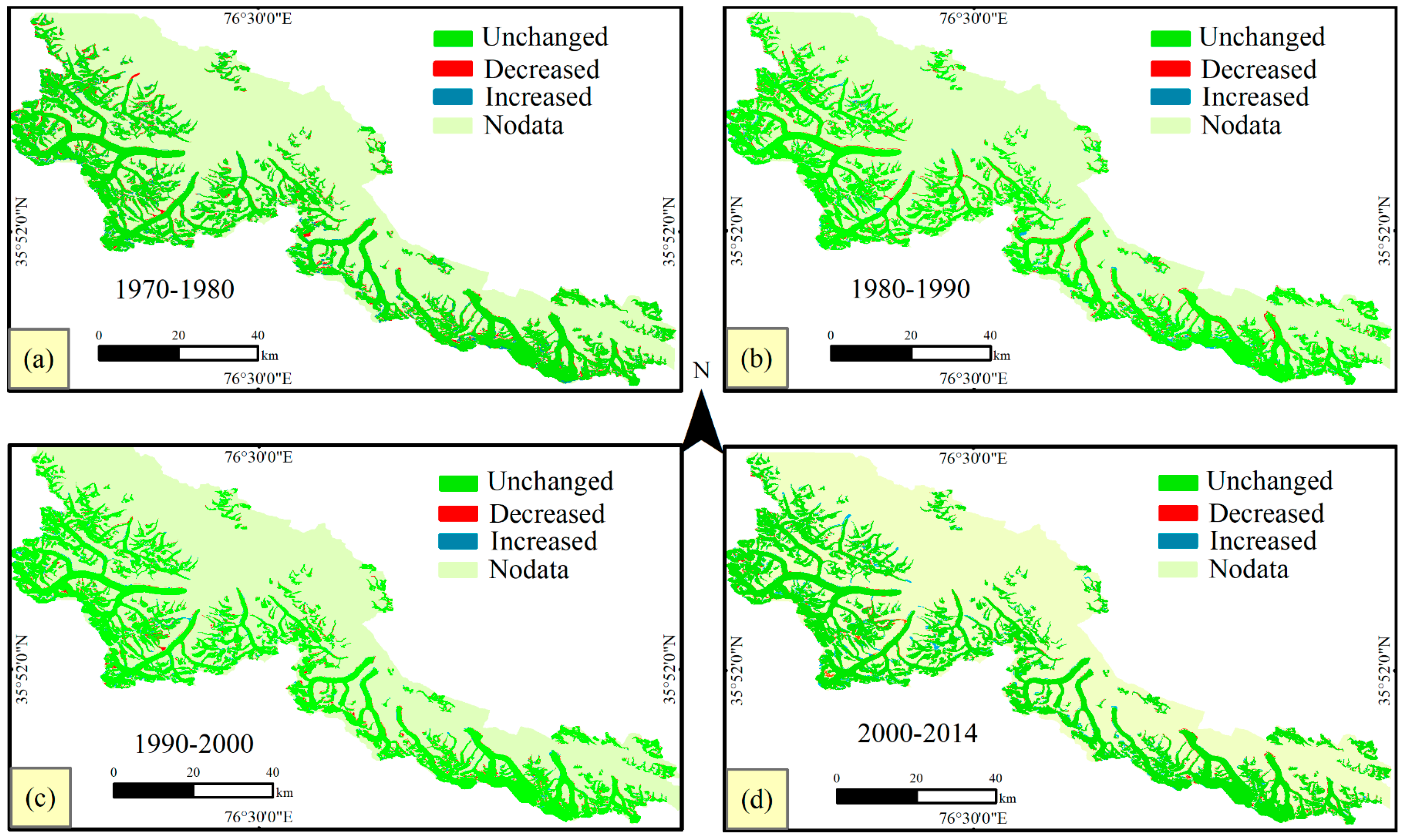
5.3. Decadal Changes in Glacier Area between 1970 and 2014
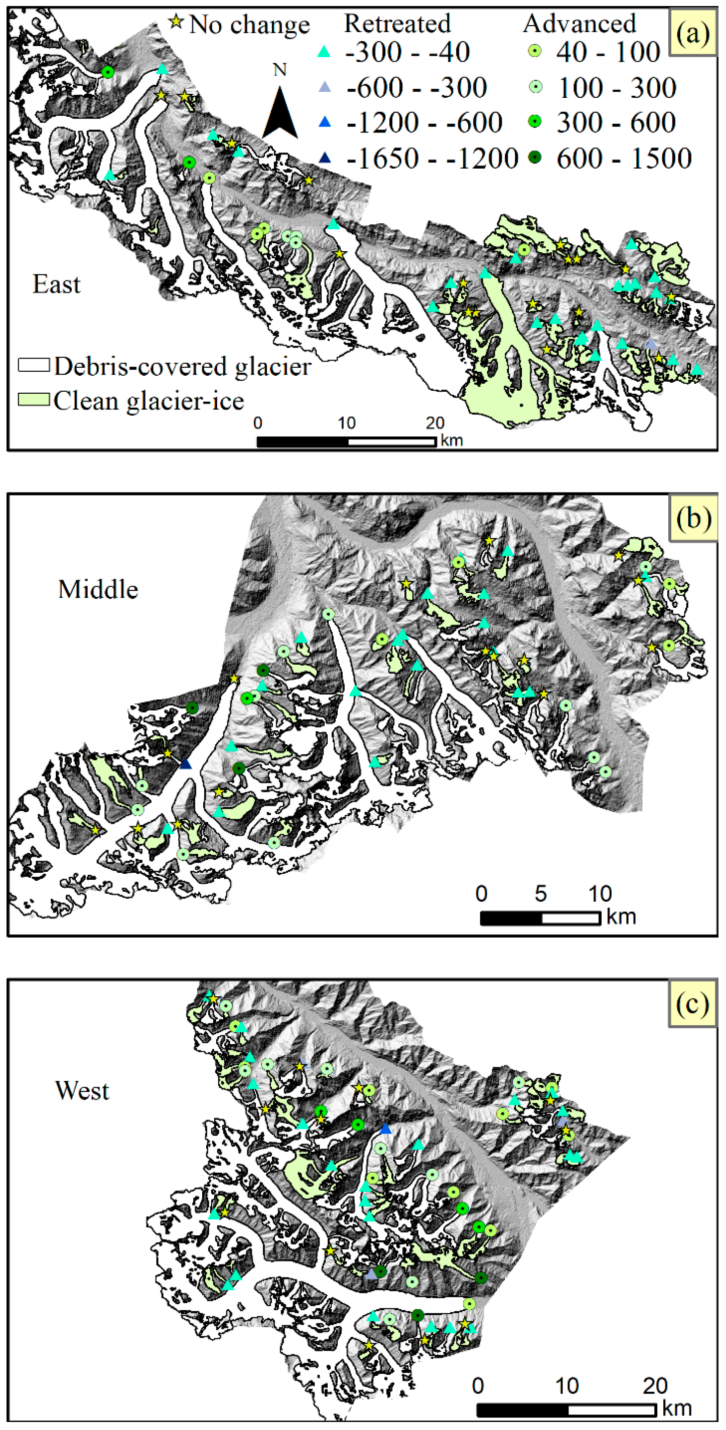
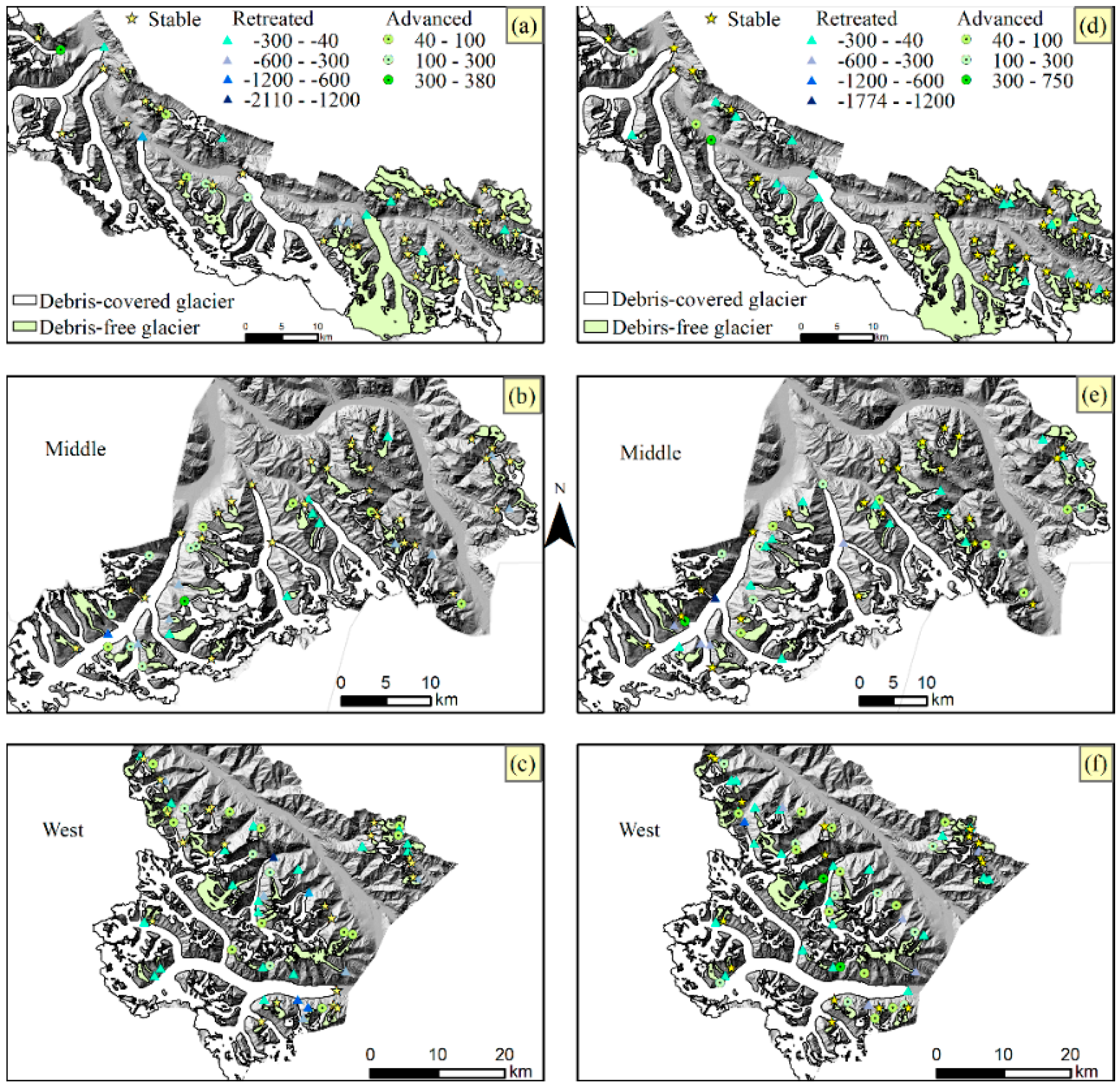
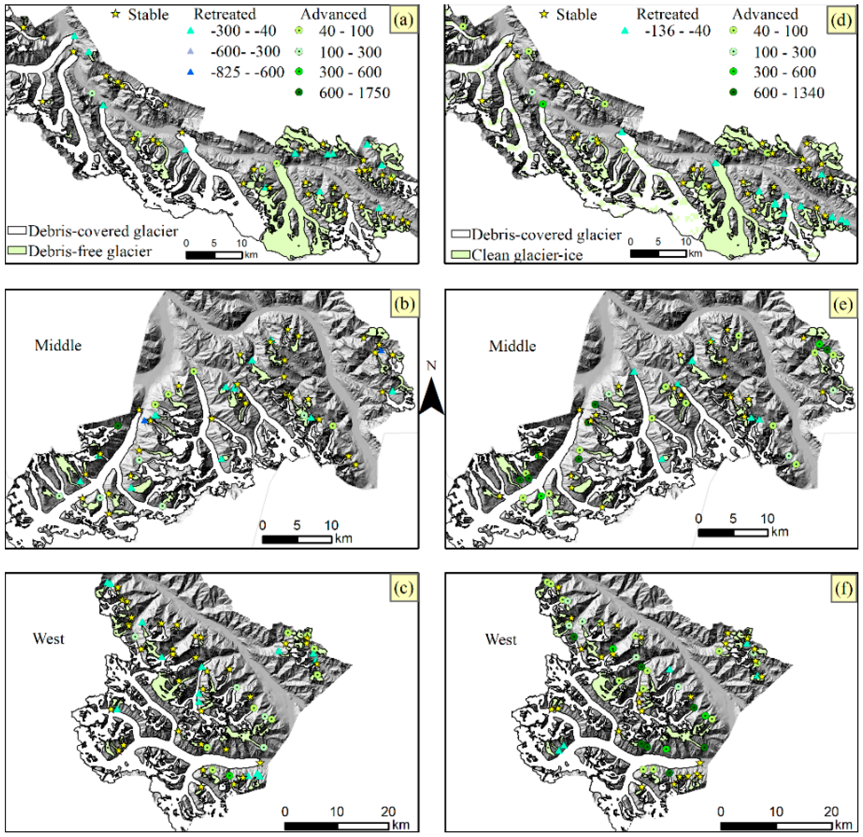
5.4. Glacier Terminus Change
6. Discussion
6.1. Glacier Change
6.2. Glacier Area Change with Glacier Topographic Parameters
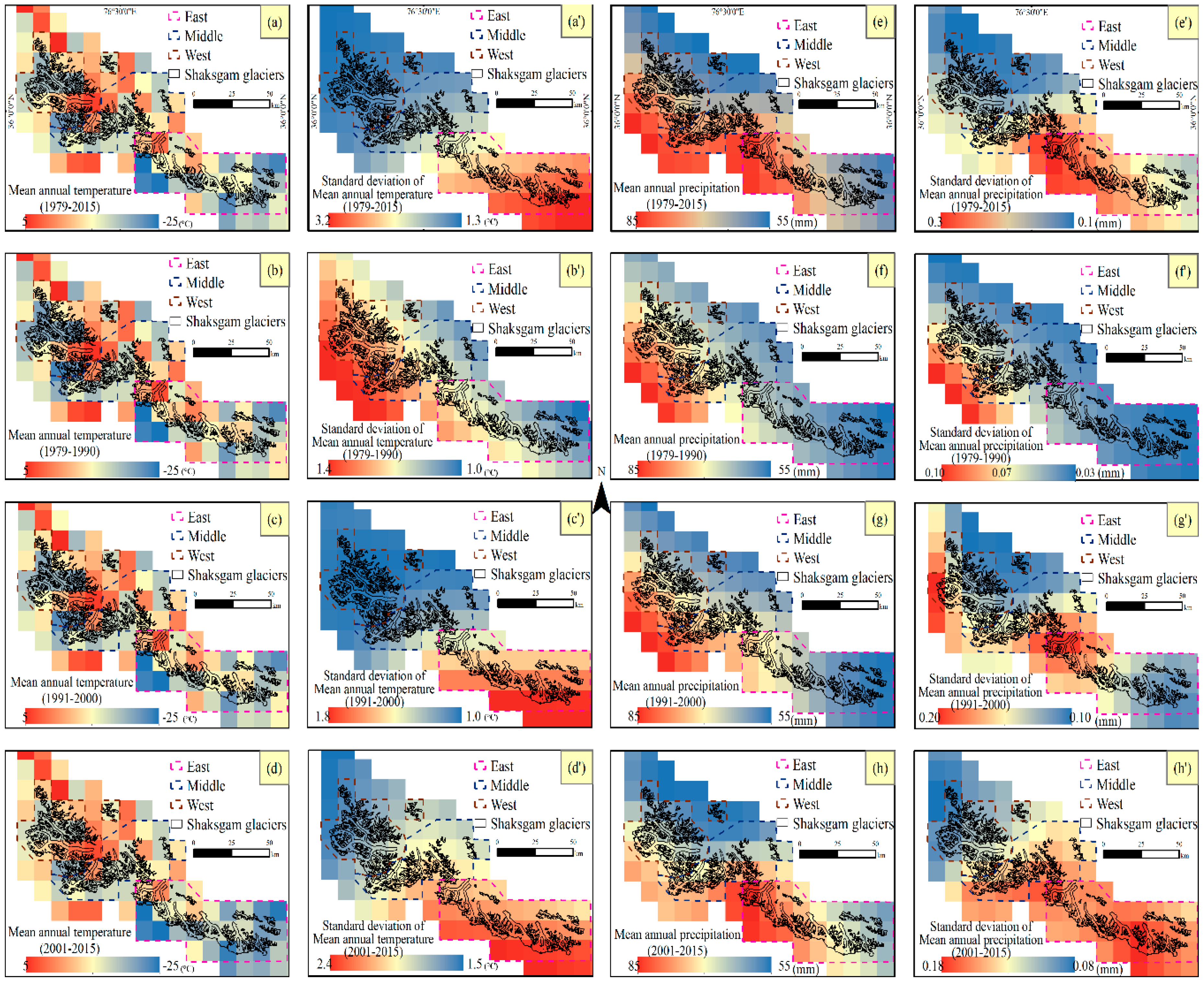
6.3. Glacier Area Change with Climate Considerations
6.4. Limitations of the Study
- Rock glaciers and ice-cored moraines are not possible to detect by the proposed method due to their much smaller size and overall area being entirely covered by rocky materials compared to the debris-covered glacier. Importantly, the thermal properties of rock glaciers and ice-cored moraines are undetectable because of a very thick deposit layer [64].
- Small hanging debris-covered glaciers had the highest uncertainty in glacier delineation mainly due to the limited image resolution. Therefore, manual editing steps are still required for small debris-covered glaciers and river channels connected with a glacier tongue and isolated areas that are outside the main body of the glacier.
7. Conclusions
Supplementary Materials
Author Contributions
Funding
Acknowledgments
Conflicts of Interest
References
- Vaughan, D.G.; Comiso, J.C.; Allison, I.; Carrasco, J.; Kaser, G.; Kwok, R.; Mote, P.; Murray, T.; Paul, F.; Ren, J.; et al. Observations: Cryosphere; Cambridge University Press: Cambridge, UK; New York, NY, USA, 2013; pp. 317–382. [Google Scholar]
- Haeberli, W.; Hoelzle, M.; Paul, F.; Zemp, M. Integrated monitoring of mountain glaciers as key indicators of global climate change: The European Alps. Ann. Glaciol. 2017, 46, 150–160. [Google Scholar] [CrossRef] [Green Version]
- Pieczonka, T.; Bolch, T.; Wei, J.F.; Liu, S.Y. Heterogeneous mass loss of glaciers in the Aksu-Tarim Catchment (Central Tien Shan) revealed by 1976 KH-9 Hexagon and 2009 SPOT-5 stereo imagery. Remote Sens. Environ. 2013, 130, 233–244. [Google Scholar] [CrossRef] [Green Version]
- Zhang, X.S. Investigation of glacier bursts of the Yarkant river in Xinjiang, China. Ann. Glaciol. 2017, 16, 135–139. [Google Scholar]
- Round, V.; Leinss, S.; Huss, M.; Haemmig, C.; Hajnsek, I. Surge dynamics and lake outbursts of Kyagar glacier, Karakoram. Cryosphere 2017, 11, 723–739. [Google Scholar] [CrossRef]
- Hewitt, K.; Liu, J.S. Ice-dammed lakes and outburst floods, Karakoram Himalaya: Historical perspectives on emerging threats. Phys. Geogr. 2010, 31, 528–551. [Google Scholar] [CrossRef]
- Kääb, A.; Treichler, D.; Nuth, C.; Berthier, E. Brief communication: Contending estimates of 2003–2008 glacier mass balance over the Pamir-Karakoram-Himalaya. Cryosphere 2015, 9, 557–564. [Google Scholar] [CrossRef]
- Bhambri, R.; Hewitt, K.; Kawishwar, P.; Pratap, B. Surge-type and surge-modified glaciers in the Karakoram. Sci. Rep. 2017. [Google Scholar] [CrossRef] [PubMed]
- Azam, M.F.; Wagnon, P.; Berthier, E.; Vincent, C.; Fujita, K.; Kargel, J.S. Review of the status and mass changes of Himalayan-Karakoram glaciers. J. Glaciol. 2018, 64, 61–74. [Google Scholar] [CrossRef] [Green Version]
- Koboltschnig, G.R.; Schoner, W.; Zappa, M.; Kroisleitner, C.; Holzmann, H.R. Runoff modelling of the glacierized Alpine Upper Salzach basin (Austria): Multi-criteria result validation. Hydrol. Process. 2008, 22, 3950–3964. [Google Scholar] [CrossRef]
- Hirabayashi, Y.; Doll, P.; Kanae, S. Global-scale modeling of glacier mass balances for water resources assessments: Glacier mass changes between 1948 and 2006. J. Hydrol. 2010, 390, 245–256. [Google Scholar] [CrossRef]
- Pfeffer, W.T.; Arendt, A.A.; Bliss, A.; Bolch, T.; Cogley, J.G.; Gardner, A.S.; Hagen, J.O.; Hock, R.; Kaser, G.; Kienholz, C.; et al. The Randolph Glacier Inventory: A globally complete inventory of glaciers. J. Glaciol. 2014, 60, 537–552. [Google Scholar] [CrossRef] [Green Version]
- Shi, Y.; Liu, S.; Ye, B.; Liu, C.; Wang, Z. Concise Glacier Inventory of China; Shanghai Popular Science Press: Shanghai, China, 2008. [Google Scholar]
- Guo, W.Q.; Liu, S.Y.; Xu, L.; Wu, L.Z.; Shangguan, D.H.; Yao, X.J.; Wei, J.F.; Bao, W.J.; Yu, P.C.; Liu, Q.; et al. The second Chinese glacier inventory: Data, methods and results. J. Glaciol. 2015, 61, 357–372. [Google Scholar] [CrossRef]
- Glaciers_cci (2015): Climate Research Data Package (CRDP) Technical Document. Available online: http://www.esa-glaciers-cci.org/ (accessed on 19 March 2018).
- Nuimura, T.; Sakai, A.; Taniguchi, K.; Nagai, H.; Lamsal, D.; Tsutaki, S.; Kozawa, A.; Hoshina, Y.; Takenaka, S.; Omiya, S.; et al. The GAMDAM glacier inventory: A quality-controlled inventory of Asian glaciers. Cryosphere 2015, 9, 849–864. [Google Scholar] [CrossRef]
- Rankl, M.; Kienholz, C.; Braun, M. Glacier changes in the Karakoram region mapped by multimission Satellite imagery. Cryosphere 2014, 8, 977–989. [Google Scholar] [CrossRef] [Green Version]
- Bolch, T.; Yao, T.; Kang, S.; Buchroithner, M.F.; Scherer, D.; Maussion, F.; Huintjes, E.; Schneider, C. A glacier inventory for the western Nyainqentanglha Range and the Nam co basin, Tibet, and glacier changes 1976–2009. Cryosphere 2010, 4, 419–433. [Google Scholar] [CrossRef]
- Racoviteanu, A.E.; Arnaud, Y.; Williams, M.W.; Manley, W.F. Spatial patterns in glacier characteristics and area changes from 1962 to 2006 in the Kanchenjunga-sikkim area, eastern Himalaya. Cryosphere 2015, 9, 505–523. [Google Scholar] [CrossRef] [Green Version]
- Kuhle, M. The maximum ice age glaciation between the Karakorum main ridge (K2) and the Tarim basin and its influence on global energy balance. J. Mt. Sci. 2005, 2, 5–22. [Google Scholar] [CrossRef]
- Bookhagen, B.; Burbank, D.W. Toward a complete Himalayan hydrological budget: Spatiotemporal distribution of snowmelt and rainfall and their impact on river discharge. J. Geophys. Res. Earth Surf. 2010, 115. [Google Scholar] [CrossRef] [Green Version]
- Jiang, Z.L.; Liu, S.Y.; Peters, J.; Lin, J.; Long, S.C.; Han, Y.S.; Wang, X. Analyzing Yengisogat Glacier surface velocities with ALOS PALSAR data feature tracking, Karakoram, China. Environ. Earth Sci. 2012, 67, 1033–1043. [Google Scholar] [CrossRef]
- Sinha, R.; Ravindra, R. Earth System Processes and Disaster Management; Sinha, R., Ravindra, R., Eds.; Springer: Berlin/Heidelberg, Germany, 2012. [Google Scholar]
- Copland, L.; Sylvestre, T.; Bishop, M.P.; Shroder, J.F.; Seong, Y.B.; Owen, L.A.; Bush, A.; Kamp, U. Expanded and recently increased glacier surging in the Karakoram. Arct. Antarct. Alp. Res. 2011, 43, 503–516. [Google Scholar] [CrossRef]
- Bhambri, R.; Bolch, T.; Kawishwar, P.; Dobhal, D.P.; Srivastava, D.; Pratap, B. Heterogeneity in glacier response in the upper Shyok valley, northeast Karakoram. Cryosphere 2013, 7, 1385–1398. [Google Scholar] [CrossRef] [Green Version]
- Sohn, H.G.; Kim, G.H.; Yom, J.H. Mathematical modelling of historical reconnaissance CORONA KH-4B imagery. Photogramm. Rec. 2004, 19, 51–65. [Google Scholar] [CrossRef]
- Surazakov, A.; Aizen, V. Positional accuracy evaluation of declassified HEXAGON KH-9 mapping camera imagery. Photogramm. Eng. Remote Sens. 2010, 76, 603–608. [Google Scholar] [CrossRef]
- Holzer, N.; Vijay, S.; Yao, T.; Xu, B.; Buchroithner, M.; Bolch, T. Four decades of glacier variations at Muztagh Ata (eastern Pamir): A multi-sensor study including HEXAGON KH-9 and Pleiades data. Cryosphere 2015, 9, 2071–2088. [Google Scholar] [CrossRef] [Green Version]
- Alifu, H.; Tateishi, R.; Johnson, B. A new band ratio technique for mapping debris-covered glaciers using Landsat imagery and a digital elevation model. Int. J. Remote Sens. 2015, 36, 2063–2075. [Google Scholar] [CrossRef]
- Alifu, H.; Johnson, B.A.; Tateishi, R. Delineation of debris-covered glaciers based on a combination of geomorphometric parameters and a TIR/NIR/SWIR band ratio. IEEE J. Sel. Top. Appl. Earth Obs. Remote Sens. 2016, 9, 781–792. [Google Scholar] [CrossRef]
- Haeberli, W.; Hoelzle, M. Application of inventory data for estimating characteristics of and regional climate-change effects on mountain glaciers: A pilot study with the European Alps. Ann. Glaciol. 1995, 21, 206–212. [Google Scholar] [CrossRef]
- Racoviteanu, A.E.; Arnaud, Y.; Williams, M.W.; Ordonez, J. Decadal changes in glacier parameters in the cordillera blanca, peru, derived from remote sensing. J. Glaciol. 2008, 54, 499–510. [Google Scholar] [CrossRef]
- Paul, F.; Frey, H.; Le Bris, R. A new glacier inventory for the European Alps from Landsat TM scenes of 2003: Challenges and results. Ann. Glaciol. 2011, 52, 144–152. [Google Scholar] [CrossRef] [Green Version]
- Tadono, T.; Takaku, J.; Tsutsui, K.; Oda, F.; Nagai, H.; IEEE. Status of “ALOS World 3D (AW3D)” Global DSM generation. In Proceedings of the 2015 IEEE International Geoscience and Remote Sensing Symposium, Milan, Italy, 26–31 July 2015; pp. 3822–3825. [Google Scholar]
- Takaku, J.; Tadono, T.; Tsutsui, K.; Ichikawa, M. Validation of ‘AW3D’ Global DSM generated from ALOS PRISM. Ann. Photogramm. Remote Sens. Spat. Inf. Sci. 2016, 3, 25–31. [Google Scholar]
- Tadono, T.; Nagai, H.; Ishida, H.; Oda, F.; Naito, S.; Minakawa, K.; Iwamoto, H. Generation of the 30 m-mesh global digital surface model by alos prism. Int. Arch. Photogramm. Remote Sens. Spat. Inf. Sci. 2016, 41, 157–162. [Google Scholar] [CrossRef]
- Wilson, A.M.; Jetz, W. Remotely sensed high-resolution global cloud dynamics for predicting ecosystem and biodiversity distributions. PLoS Biol. 2016, 14, e1002415. [Google Scholar] [CrossRef] [PubMed]
- Chen, Y.Y.; Yang, K.; He, J.; Qin, J.; Shi, J.C.; Du, J.Y.; He, Q. Improving land surface temperature modeling for dry land of China. J. Geophys. Res. Atmos. 2011, 116. [Google Scholar] [CrossRef] [Green Version]
- He, J.; Yang, K. China Meteorological Forcing Dataset. Cold and Arid Regions Science Data Center at Lanzhou. Available online: http://westdc.westgis.ac.cn/data/7a35329c-c53f-4267-aa07-e0037d913a21 (accessed on 12 March 2018).
- Müller, F.; Caflisch, T.; Müller, G. Instructions for Compilation and Assemblage of Data for a World Glacier Inventory. Available online: https://wgms.ch/downloads/Mueller_etal_UNESCO_1977.pdf (accessed on 12 June 2018).
- Fischer, M.; Huss, M.; Barboux, C.; Hoelzle, M. The New Swiss Glacier Inventory sgi2010: Relevance of Using High-resolution Source Data in Areas Dominated by Very Small Glaciers. Arct. Antarct. Alp. Res. 2014, 46, 933–945. [Google Scholar] [CrossRef]
- Toutin, T. Aster DEMs for geomatic and geoscientific applications: A review. Int. J. Remote Sens. 2008, 29, 1855–1875. [Google Scholar] [CrossRef]
- Paul, F.; Barry, R.G.; Cogley, J.G.; Frey, H.; Haeberli, W.; Ohmura, A.; Ommanney, C.S.L.; Raup, B.; Rivera, A.; Zemp, M. Recommendations for the compilation of glacier inventory data from digital sources. Ann. Glaciol. 2009, 50, 119–126. [Google Scholar] [CrossRef] [Green Version]
- RGI Consortium. Randolph Glacier Inventory-A Dataset of Global Glacier Outlines: Version 6.0. Available online: http://www.glims.org/RGI/randolph60.html (accessed on 28 July 2017).
- Bolch, T.; Menounos, B.; Wheate, R. Landsat-based inventory of glaciers in western Canada, 1985–2005. Remote Sens. Environ. 2010, 114, 127–137. [Google Scholar] [CrossRef]
- Tennant, C.; Menounos, B.; Wheate, R.; Clague, J.J. Area change of glaciers in the Canadian Rocky Mountains, 1919 to 2006. Cryosphere 2012, 6, 1541–1552. [Google Scholar] [CrossRef] [Green Version]
- Hall, D.K.; Bayr, K.J.; Schoner, W.; Bindschadler, R.A.; Chien, J.Y.L. Consideration of the errors inherent in mapping historical glacier positions in Austria from the ground and space (1893–2001). Remote Sens. Environ. 2003, 86, 566–577. [Google Scholar] [CrossRef]
- Chand, P.; Sharma, M.C. Glacier changes in the Ravi basin, North-Western Himalaya (India) during the last four decades (1971–2010/13). Glob. Planet. Chang. 2015, 135, 133–147. [Google Scholar] [CrossRef]
- Bolch, T.; Kulkarni, A.; Kaab, A.; Huggel, C.; Paul, F.; Cogley, J.G.; Frey, H.; Kargel, J.S.; Fujita, K.; Scheel, M.; et al. The state and fate of Himalayan glaciers. Science 2012, 336, 310–314. [Google Scholar] [CrossRef] [PubMed] [Green Version]
- Hewitt, K. The karakoram anomaly? Glacier expansion and the ‘elevation effect’, Karakoram Himalaya. Mt. Res. Dev. 2005, 25, 332–340. [Google Scholar] [CrossRef]
- Rankl, M.; Braun, M. Glacier elevation and mass changes over the central Karakoram region estimated from TanDEM-X and SRTM/X-SAR digital elevation models. Ann. Glaciol. 2016, 57, 273–281. [Google Scholar] [CrossRef] [Green Version]
- Zhou, Y.; Li, Z.; Li, J. Slight glacier mass loss in the Karakoram region during the 1970s to 2000 revealed by KH-9 images and SRTM DEM. J. Glaciol. 2017, 63, 331–342. [Google Scholar] [CrossRef] [Green Version]
- Liu, S.; Ding, Y.; Shangguan, D.; Zhang, Y.; Li, J.; Han, H.; Wang, J.; Xie, C. Glacier retreat as a result of climate warming and increased precipitation in the Tarim river basin, northwest China. Ann. Glaciol. 2006, 43, 91–96. [Google Scholar] [CrossRef]
- Forsythe, N.; Hardy, A.J.; Fowler, H.J.; Blenkinsop, S.; Kilsby, C.G.; Archer, D.R.; Hashmi, M.Z. A Detailed Cloud Fraction Climatology of the Upper Indus Basin and Its Implications for Near-Surface Air Temperature. J. Clim. 2015, 28, 3537–3556. [Google Scholar] [CrossRef]
- Bashir, F.; Zeng, X.B.; Gupta, H.; Hazenberg, P. A hydrometeorological perspective on the Karakoram anomaly using unique valley-based synoptic weather observations. Geophys. Res. Lett. 2017, 44, 10470–10478. [Google Scholar] [CrossRef]
- Chen, Y.N.; Xu, C.C.; Hao, X.M.; Li, W.H.; Chen, Y.P.; Zhu, C.G.; Ye, Z.X. Fifty-year climate change and its effect on annual runoff in the Tarim river basin, China. Quat. Int. 2009, 208, 53–61. [Google Scholar]
- Wang, Q.Y.; Yi, S.; Sun, W.K. P Precipitation-driven glacier changes in the Pamir and Hindu Kush mountains. Geophys. Res. Lett. 2017, 44, 2817–2824. [Google Scholar] [CrossRef]
- Li, B.F.; Chen, Y.N.; Shi, X.; Chen, Z.S.; Li, W.H. Temperature and precipitation changes in different environments in the arid region of northwest China. Theor. Appl. Climatol. 2013, 112, 589–596. [Google Scholar] [CrossRef]
- Reid, H. The mechanics of glaciers. J. Geol. 1896, 4, 912–928. [Google Scholar] [CrossRef]
- Salinger, J.; Chinn, T.; Willsman, A.; Fitzharris, B. Glacier response to climate change. Water Atmos. 2008, 16, 16–17. [Google Scholar]
- Yang, J.; Liu, S.; Tan, C. Vulnerability of mountain glaciers in China to climate change. Adv. Clim. Chang. Res. 2015, 6, 171–180. [Google Scholar] [CrossRef]
- Quincey, D.J.; Braun, M.; Glasser, N.F.; Bishop, M.P.; Hewitt, K.; Luckman, A. Karakoram glacier surge dynamics. Geophys. Res. Lett. 2011, 38. [Google Scholar] [CrossRef] [Green Version]
- Alifu, H.; Tateishi, R.; Nduati, E.; Maitiniyazi, A. Glacier changes in Glacier Bay, Alaska, during 2000–2012. Int. J. Remote Sens. 2016, 37, 4132–4147. [Google Scholar] [CrossRef]
- Owen, L.A.; England, J. Observations on rock glaciers in the Himalayas and Karakoram Mountains of northern Pakistan and India. Geomorphology 1998, 26, 199–213. [Google Scholar] [CrossRef] [Green Version]


| Satellite | Scenes ID | Date (dd/mm/yy) | Resolution | Spectral Band | Utilization |
|---|---|---|---|---|---|
| Corona KH-4A | DS1025-1039DA015 | 08/10/1965 | 3.5 m | 1 panchromatic band (PAN) | Glacier inventory for 1970 |
| Corona KH-4A | DS1044-1023DA019 | 04/11/1967 | |||
| Corona KH-4B | DS1107-1104DA005 | 30/07/1969 | |||
| Corona KH-4B | DS1107-1104DA003 | 30/07/1969 | |||
| Corona KH-4B | DS1107-1104DA002 | 30/07/1969 | |||
| Corona KH-4B | DS1107-1104DA004 | 30/07/1969 | |||
| Corona KH-4B | DS1107-1104DA003 | 30/07/1969 | |||
| Corona KH-4B | DS1107-1104DA005 | 30/07/1969 | |||
| Corona KH-4B | DS1115-1088DF201 | 16/09/1971 | |||
| Corona KH-4B | DS1115-1088DF202 | 16/09/1971 | |||
| Corona KH-4B | DS1115-1088DF203 | 16/09/1971 | |||
| Corona KH-4B | DS1115-1088DF204 | 16/09/1971 | |||
| Hexagon KH-9 | DZB1216-500018L009001 | 22/07/1980 | 7.5 m | 1 PAN | Glacier inventory for 1980 |
| Hexagon KH-9 | DZB1216-500361L006001 | 16/09/1980 | |||
| Landsat TM | ETP148R35_5T19900629 | 29/06/1990 | 28.5 m 120 m | 3 visible (VIS), 1 near-infrared (NIR), 2 shortwave infrared (SWIR), 1 thermal infrared (TIR) | Glacier inventory for 1990 |
| Landsat TM | LT51480351993188ISP00 | 07/07/1993 | 30 m 120 m | 3 VIS, 1 NIR, 2 SWIR, 1 TIR | Additional information for glacier identification (1990) |
| SRTM | SRTM3N35E075V2 SRTM3N35E076V2 SRTM3N36E075V2 SRTM3N36E076V2 SRTM3N36E077V2 SRTM3N35E077V2 | 02/2000 | 30 m | Additional information (Slope) for glacier identification (1990) Additional information (slope, plan curvature and profile curvature) for glacier identification (2000) | |
| Landsat ETM+ | LE71480352000168SGS01 | 16/06/2000 | 15 m 30 m 60 m | 1 PAN 3 VIS, 1 NIR, 2 SWIR, 1 TIR | Glacier inventory for 2000 |
| Landsat ETM+ | LE71480352001202SGS00 | 21/07/2001 | 15 m 30 m 60 m | 1 PAN 3 VIS, 1 NIR, 2 SWIR, 1 TIR | Additional information for glacier identification (2000) |
| Landsat OLI/TIRS | LC81480352014166LGN00 | 15/06/2014 | 15 m 30 m 100 m | 1 PAN 3 VIS, 1 NIR, 2 SWIR, 1 TIR | Glacier inventory for 2014 |
| Landsat OLI/TIRS | LC81480352015185LGN00 | 04/07/2015 | 15 m 30 m 100 m | 1 PAN 3 VIS, 1 NIR, 2 SWIR, 1 TIR | Additional information for glacier identification (2014) |
| Terra ASTER | 148-101-5_051020_L1A | 20/10/2005 | 15 m 30 m 90 m | 2 VIS, 2 NIR 6 SWIR 4 TIR | DEM generation and extracting additional information (slope, plan curvature and profile curvature) for glacier identification (2014) |
| Terra ASTER | 148-101-4_110428_L1A | 28/04/2011 | |||
| Terra ASTER | 149-100-7_110505_L1A | 05/05/2011 | |||
| Terra ASTER | 147-102-2_110608_L1A | 08/06/2011 | |||
| Terra ASTER | 148-101-5_120703_L1A | 03/07/2012 | |||
| Terra ASTER | 148-100-2_140725_L1A | 25/07/2014 | |||
| Terra ASTER | 148-101-2_140725_L1A | 25/07/2014 | |||
| AW3D30 | N035E076 N035E077 N036E075 N036E076 | 2006–2011 | 30 m | Glacier parameters extraction | |
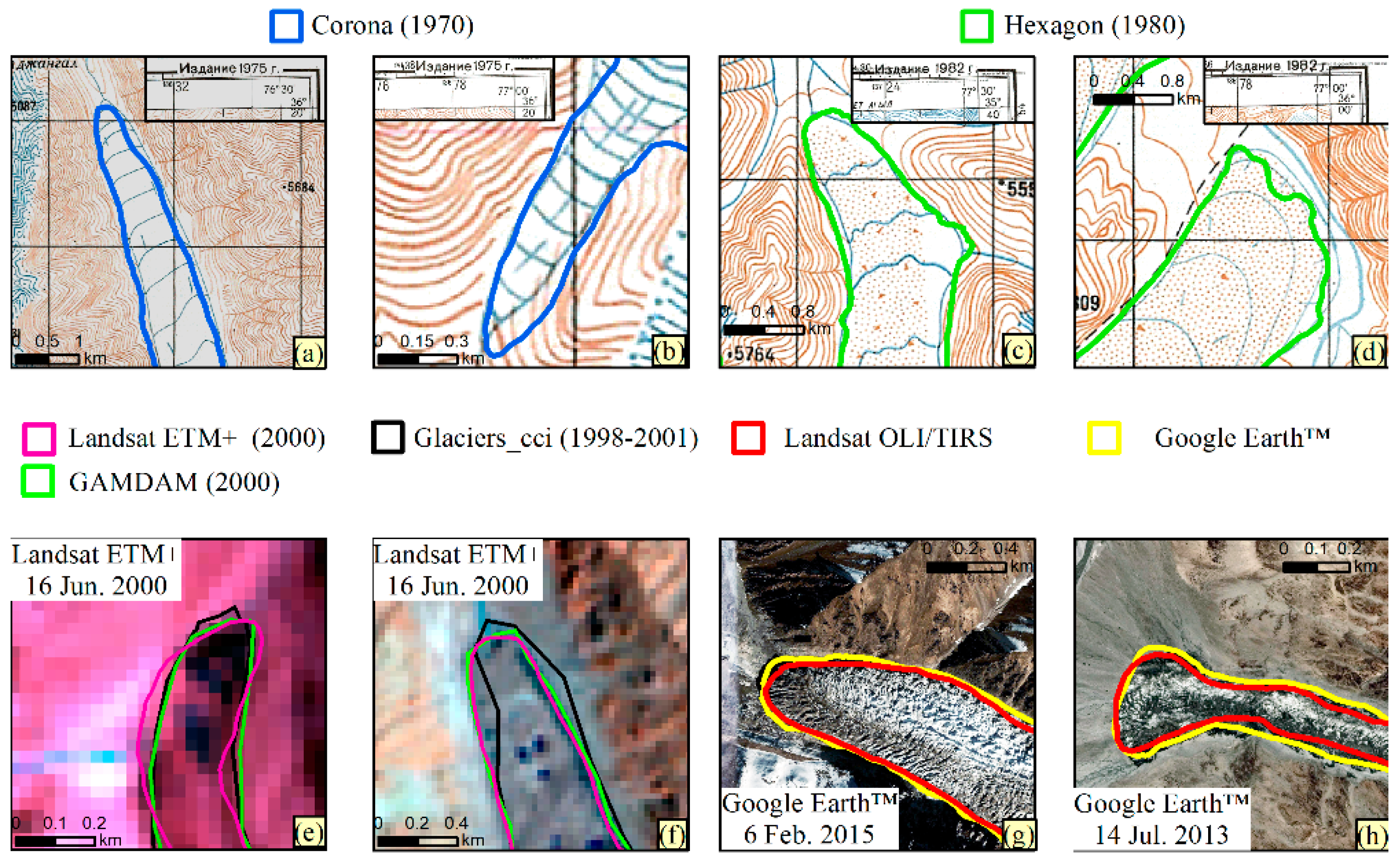
| Soviet Military Topo maps | 3 maps 7 maps | 1975 1982 | 1:100,000 | Comparisons for glacier inventory 1970–1980 | |
| GAMDAM Glacier Inventory | 2000 | 30 m | Comparisons for glacier inventory 2000 | ||
| Glaciers_cci | 2000 | 30 m | Comparisons for glacier inventory 2000 | ||
| Google Earth™ Images | 2014 | 2–5 m | Comparisons for glacier inventory 2014 |
| DEMs | Total Points Number | Min | Max | Mean | DEMthis study RMSE |
|---|---|---|---|---|---|
| DEMthis study | 109 | 3565 | 5360 | 4485 | / |
| SRTM | 109 | 3580 | 5356 | 4484 | 13 |
| ASTER GDEM | 109 | 3570 | 5377 | 4480 | 12 |
| AW3DS30 | 109 | 3580 | 5336 | 4481 | 13 |
| Year | Errorarea Year (%) | Period | Errorarea Period (%) | Errorterminus Period (m) |
|---|---|---|---|---|
| 1970 | 2.0 | 1970–1980 | 3.5 | 20.0 |
| 1980 | 2.9 | 1980–1990 | 4.3 | 42.0 |
| 1990 | 3.2 | 1990–2000 | 4.0 | 52.0 |
| 2000 | 2.4 | 2000–2014 | 3.3 | 50.0 |
| 2014 | 2.3 | 1970–2014 | 3.0 | 37.0 |
| Inventory | Overall | Debris-Free Glacier | Debris-Covered Glacier | ||||||
|---|---|---|---|---|---|---|---|---|---|
| Min | Max | Mean | Min | Max | Mean | Min | Max | Mean | |
| Min elevation (m) | 3972.0 | 5922.0 | 4960.0 | 4043.0 | 5922.0 | 5083.0 | 3972.0 | 5215.0 | 4676.0 |
| Max elevation (m) | 5560.0 | 7901.0 | 6168.0 | 5581.0 | 7207.0 | 6089.0 | 5560.0 | 7901.0 | 6351.0 |
| Median elevation (m) | 5013.0 | 6058.0 | 5579.0 | 5201.0 | 6058.0 | 5628.0 | 5013.0 | 5794.0 | 5464.0 |
| Slope (°) | 15.0 | 43.0 | 26.0 | 15.0 | 43.0 | 27.0 | 15.0 | 36.0 | 24.0 |
| Area (km2) | 0.5 | 344.6 | 8.5 | 0.5 | 84.7 | 2.4 | 0.6 | 344.6 | 22.8 |
| Debris cover (km2) | - | - | 0.03 | 41.5 | 2.5 | ||||
| Number of glacier | 173 | 121 | 52 | ||||||
| Total Area (km2) | 1478 | 295 | 1184 | ||||||
| Comparison | TGN | Total GA | Mean GA | SDGA | |
|---|---|---|---|---|---|
| 1970 | Overall | 176 | 1501 | 8.5 | 30.8 |
| Debris-free glacier | 123 | 329 | 2.7 | 8.2 | |
| Debris-covered glacier | 53 | 1171 | 22.1 | 52.3 | |
| 1980 | Overall | 177 | 1507 | 8.5 | 30.9 |
| Debris-free glacier | 123 | 327 | 2.7 | 8.2 | |
| Debris-covered glacier | 54 | 1180 | 21.9 | 52.2 | |
| 1990 | Overall | 173 | 1451 | 8.4 | 30.5 |
| Debris-free glacier | 120 | 291 | 2.4 | 7.9 | |
| Debris-covered glacier | 53 | 1159 | 21.9 | 51.4 | |
| 2000 | Overall | 173 | 1446 | 8.4 | 30.8 |
| Debris-free glacier | 120 | 289 | 2.4 | 7.8 | |
| Debris-covered glacier | 53 | 1157 | 21.8 | 51.9 | |
| 2014 | Overall | 173 | 1478 | 8.5 | 31.4 |
| Debris-free glacier | 121 | 295 | 2.4 | 7.7 | |
| Debris-covered glacier | 52 | 1184 | 22.8 | 53.5 | |
| Regression | R Square | Coefficient | p Value |
|---|---|---|---|
| Glacier area | 0.087 | 0.042 | 0.590 |
| Min elevation | −0.001 | 0.817 | |
| Max elevation | 0.001 | 0.898 | |
| Median elevation | 0.002 | 0.684 | |
| Slope | −0.134 | 0.196 | |
| Aspect | −0.003 | 0.929 | |
| Debris-cover | 0.016 | 0.101 | 0.110 |
| Regression | R Square | Coefficient | p Value | R Square | Coefficient | p Value |
|---|---|---|---|---|---|---|
| Glacier area | 0.172 | −2.417 | 0.050 | 0.264 | −2.103 | 0.414 |
| Min elevation | −0.401 | 0.155 | −0.725 | 2.542 | ||
| Max elevation | −0.206 | 0.304 | −0.177 | 0.211 | ||
| Median elevation | 0.296 | 0.462 | 0.465 | 0.058 | ||
| Slope | −2.373 | 0.796 | −6.110 | 0.252 | ||
| Aspect | −0.202 | 0.586 | −0.212 | 0.303 |
© 2018 by the authors. Licensee MDPI, Basel, Switzerland. This article is an open access article distributed under the terms and conditions of the Creative Commons Attribution (CC BY) license (http://creativecommons.org/licenses/by/4.0/).
Share and Cite
Alifu, H.; Hirabayashi, Y.; Johnson, B.A.; Vuillaume, J.-F.; Kondoh, A.; Urai, M. Inventory of Glaciers in the Shaksgam Valley of the Chinese Karakoram Mountains, 1970–2014. Remote Sens. 2018, 10, 1166. https://doi.org/10.3390/rs10081166
Alifu H, Hirabayashi Y, Johnson BA, Vuillaume J-F, Kondoh A, Urai M. Inventory of Glaciers in the Shaksgam Valley of the Chinese Karakoram Mountains, 1970–2014. Remote Sensing. 2018; 10(8):1166. https://doi.org/10.3390/rs10081166
Chicago/Turabian StyleAlifu, Haireti, Yukiko Hirabayashi, Brian Alan Johnson, Jean-Francois Vuillaume, Akihiko Kondoh, and Minoru Urai. 2018. "Inventory of Glaciers in the Shaksgam Valley of the Chinese Karakoram Mountains, 1970–2014" Remote Sensing 10, no. 8: 1166. https://doi.org/10.3390/rs10081166