Quadratic Frequency Modulation Signals Parameter Estimation Based on Two-Dimensional Product Modified Parameterized Chirp Rate-Quadratic Chirp Rate Distribution

Abstract
:1. Introduction
2. The 2D-PMPCRD Method
2.1. The Principle of 2D-PMPCRD
2.2. Implementation of the 2D-PMPCRD
3. Cross-Term Suppression Performance Analysis
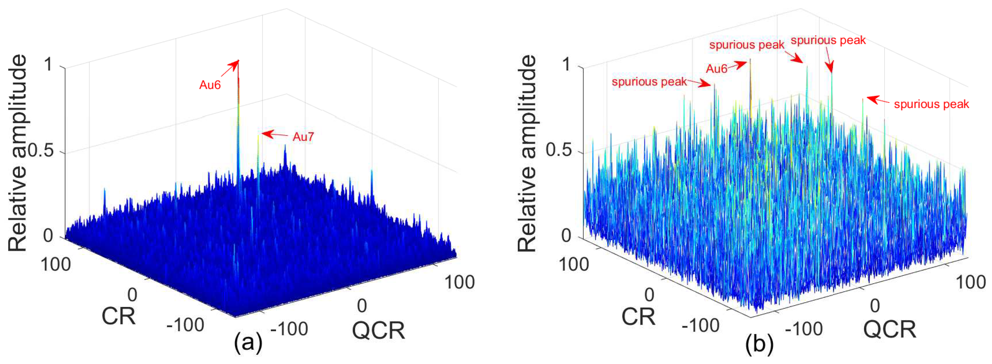
3.1. Cross-Term Suppression Comparison
- , , ,
- , , .
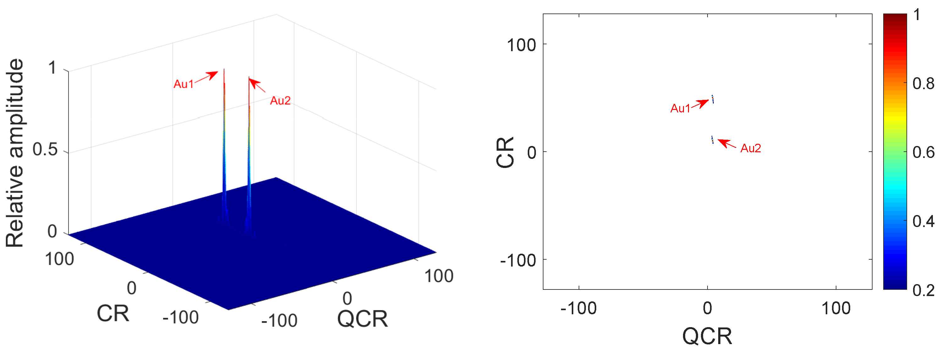
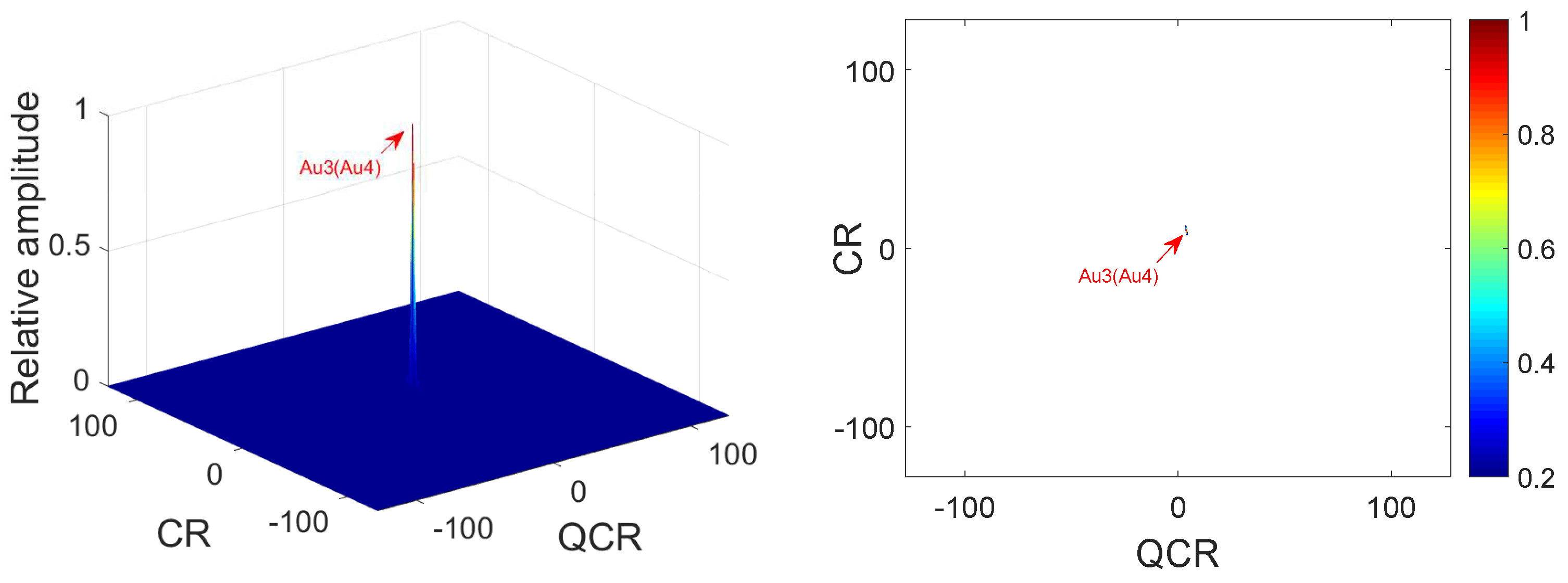
3.1.1. Case One
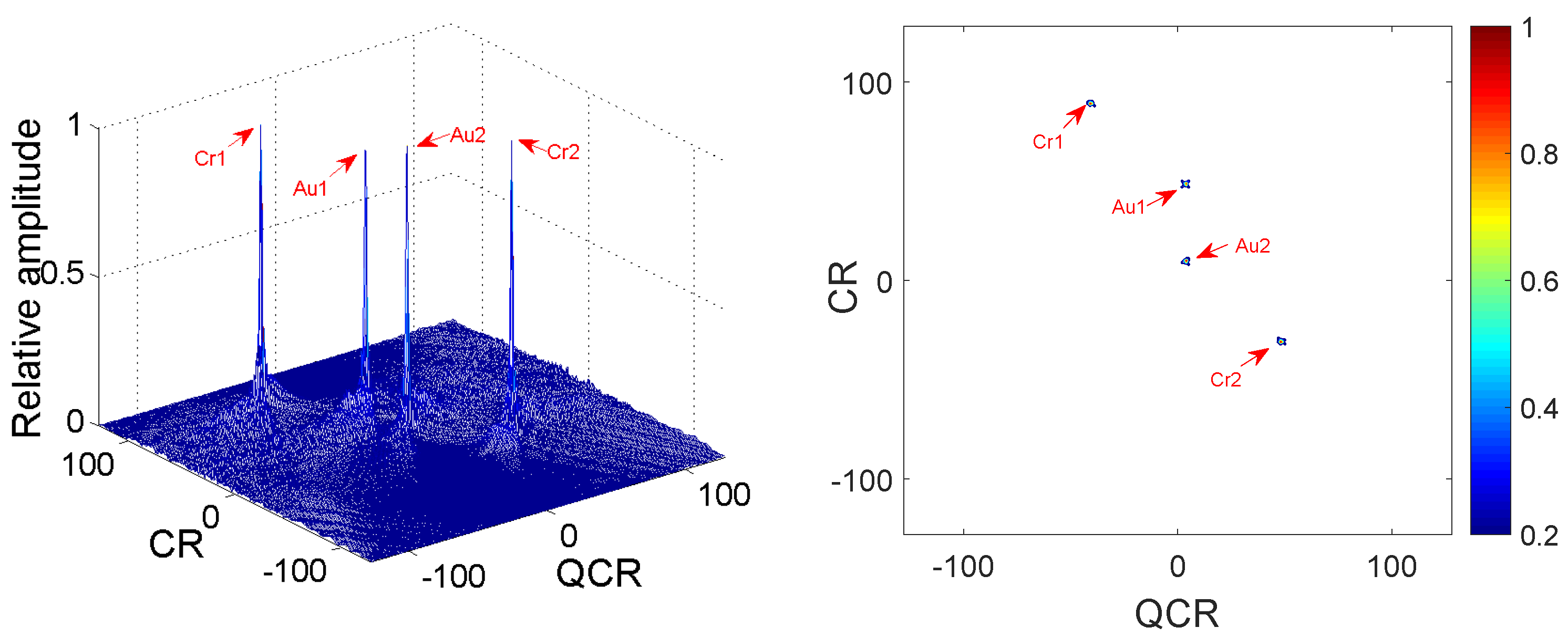
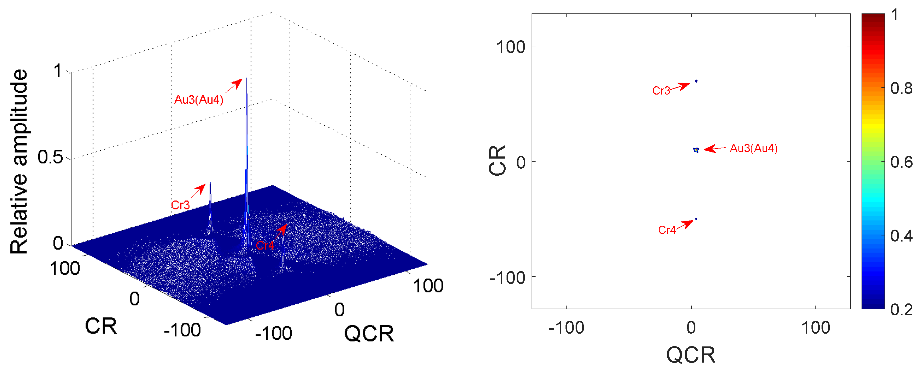
3.1.2. Case Two
3.2. Parameter Selection Criterion
3.2.1. Selection of Constant Delay
3.2.2. Selection of the Scales Factors and Number of Scale Factors
4. Anti-Noise Performance and Computation Cost Analysis
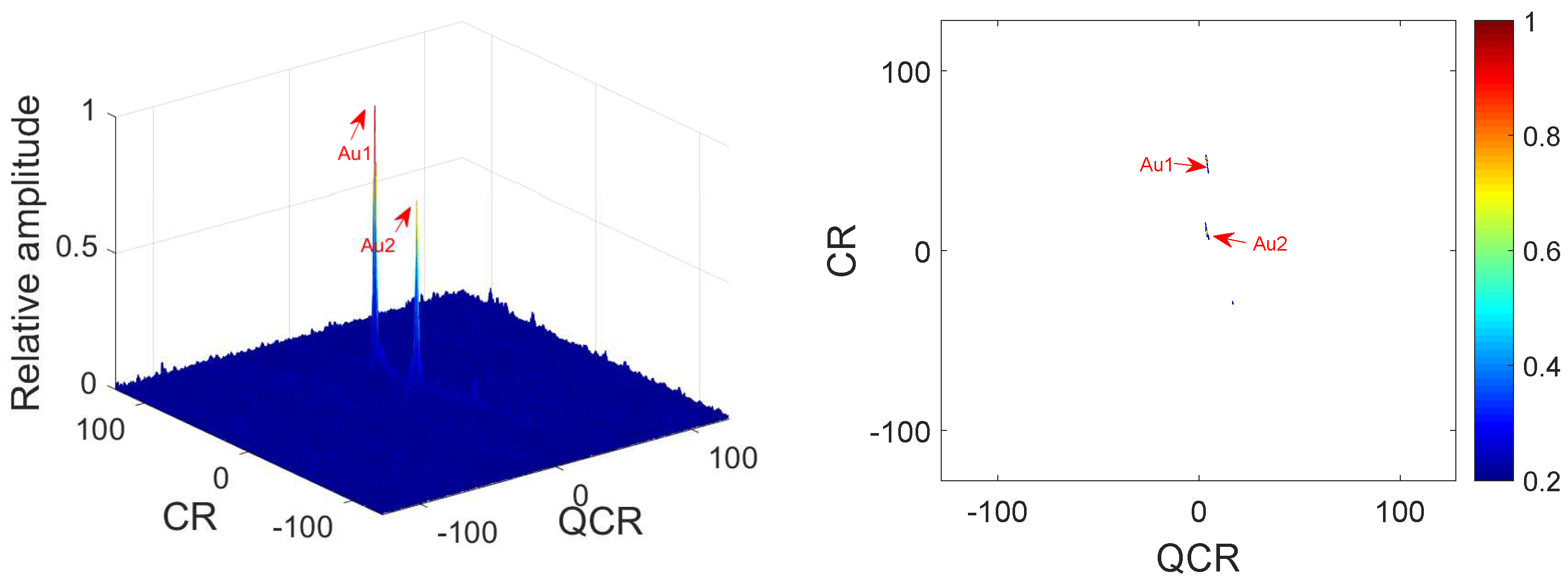
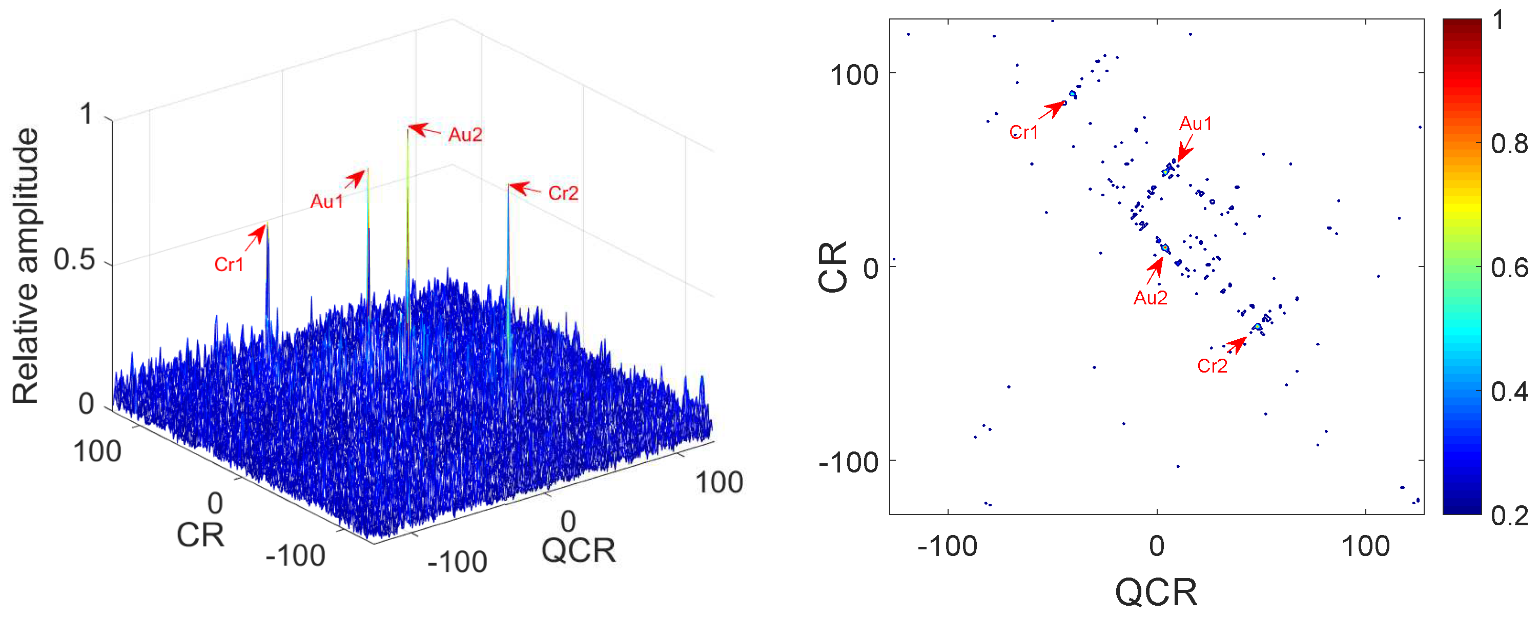
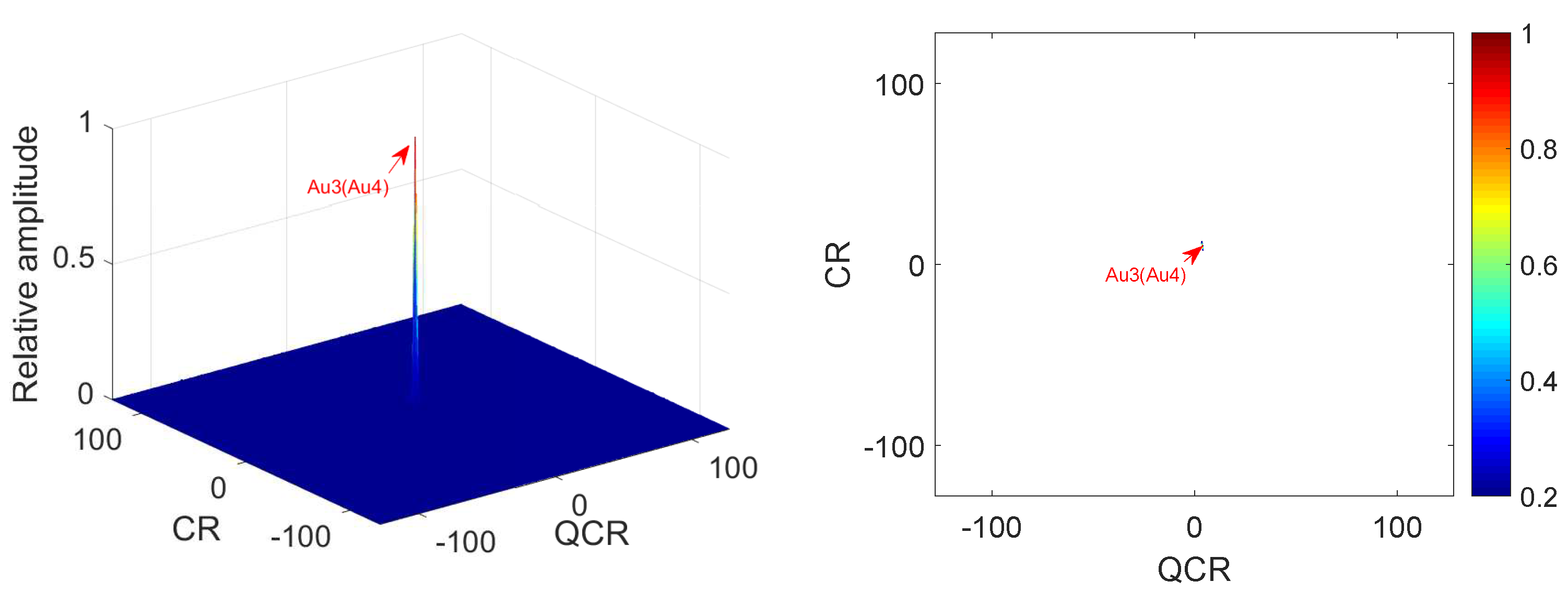
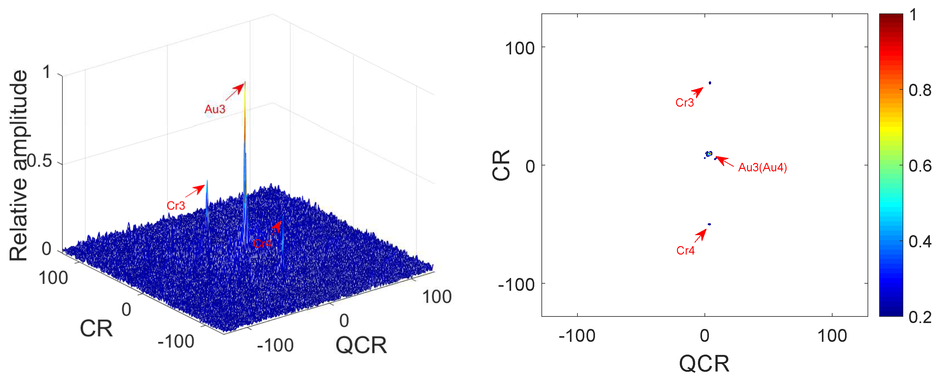
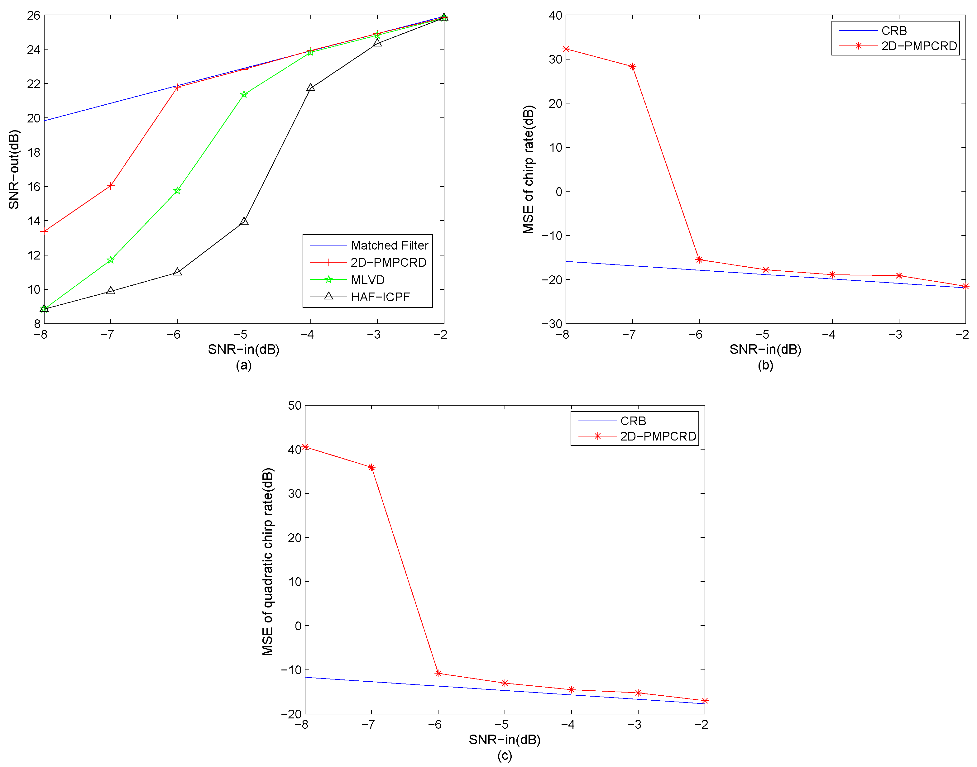
4.1. Anti-Noise Performance Analysis
4.2. Computation Cost Analysis
5. Conclusions
Author Contributions
Funding
Conflicts of Interest
References
- Lazarov, A.; Minchev, C. ISAR geometry, signal model, and image processing algorithms. IET Radar Sonar Navig. 2017, 11, 1425–1434. [Google Scholar] [CrossRef]
- Lazarov, A. ISAR signal formation and image reconstruction as complex spatial transforms. In Digital Image Processing; InTech: London, UK, 2012; pp. 27–50. [Google Scholar]
- Xing, M.; Bao, Z. High resolution ISAR imaging of high speed moving targets. IEE Proc. Radar Sonar Navig. 2005, 152, 58–67. [Google Scholar] [CrossRef]
- Wang, J.; Kasilingam, D. Global range alignment for ISAR. IEEE Trans. Aerosp. Electron. Syst. 2003, 39, 351–357. [Google Scholar] [CrossRef]
- Zhu, D.; Li, Y.; Zhu, Z. A keystone transform without interpolation for SAR ground moving-target imaging. IEEE Geosci. Remote Sens. Lett. 2007, 4, 18–22. [Google Scholar] [CrossRef]
- Xing, M.; Wu, R.; Lan, J.; Zheng, B. Migration through resolution cell compensation in ISAR imaging. IEEE Geosci. Remote Sens. Lett. 2004, 1, 141–144. [Google Scholar] [CrossRef]
- Xing, M.; Wu, R.; Li, Y.; Bao, Z. New ISAR imaging algorithm based on modified Wigner–Ville distribution. IET Radar Sonar Navig. 2009, 3, 70–80. [Google Scholar] [CrossRef]
- Almeida, L.B. The fractional fourier transform and time-frequency representations. IEEE Trans. Signal Process. 1994, 42, 3084–3091. [Google Scholar] [CrossRef]
- Shea, P.O. A new technique for instantaneous frequency rate estimation. IEEE Signal Process. Lett. 2002, 9, 251–252. [Google Scholar] [CrossRef] [Green Version]
- Lv, X.; Bi, G.; Wan, C.; Xing, M. Lv’s distribution: Principle, implementation, properties, and performance. IEEE Trans. Signal Process. 2011, 59, 3576–3591. [Google Scholar] [CrossRef]
- Zheng, J.; Liu, H.; Liu, Q.H. Parameterized centroid frequency-chirp rate distribution for LFM signal analysis and mechanisms of constant delay introduction. IEEE Trans. Signal Process. 2017, 65, 6435–6447. [Google Scholar] [CrossRef]
- Abatzoglou, T.J. Fast maximum likelihood joint estimation of frequency and frequency rate. IEEE Trans. Aerosp. Electron. Syst. 1986, 22, 708–715. [Google Scholar] [CrossRef]
- Zheng, J. Fast Parameter Estimation Algorithm for Cubic Phase Signal Based on Quantifying Effects of Doppler Frequency Shift. Prog. Electromagn. Res. 2013, 142, 57–74. [Google Scholar] [CrossRef]
- Barbarossa, S.; Petrone, V. Analysis of polynomial-phase signals by the integrated generalized ambiguity function. IEEE Trans. Signal Process. 1997, 45, 316–327. [Google Scholar] [CrossRef]
- Djurovic, I.; Simeunovic, M.; Djukanovic, S.; Wang, P. A hybrid CPF-HAF estimation of polynomial-phase signals: Detailed statistical analysis. IEEE Trans. Signal Process. 2012, 60, 5010–5023. [Google Scholar] [CrossRef]
- Shea, P.O. A fast algorithm for estimating the parameters of a quadratic FM signal. IEEE Trans. Signal Process. 2004, 52, 385–393. [Google Scholar] [CrossRef] [Green Version]
- Barbarossa, S.; Scaglione, A.; Giannakis, G.B. Product high-order ambiguity function for multicomponent polynomial-phase signal modeling. IEEE Trans. Signal Process. 1998, 46, 691–708. [Google Scholar] [CrossRef]
- Wang, P.; Yang, J. Multicomponent chirp signals analysis using product cubic phase function. Digit. Signal Process. 2006, 16, 654–669. [Google Scholar] [CrossRef]
- Wang, Y.; Jiang, Y. Inverse synthetic aperture radar imaging of maneuvering target based on the product generalized cubic phase function. IEEE Geosci. Remote Sens. Lett. 2011, 8, 958–962. [Google Scholar] [CrossRef]
- Zheng, J.; Su, T.; Zhu, W.; Zhang, L.; Liu, Z.; Liu, Q.H. ISAR imaging of nonuniformly rotating target based on a fast parameter estimation algorithm of cubic phase signal. IEEE Trans. Geosci. Remote Sens. 2015, 53, 4727–4740. [Google Scholar] [CrossRef]
- Li, Y.; Su, T.; Zheng, J.; He, X. ISAR imaging of targets with complex motions based on modified Lv’s distribution for cubic phase signal. IEEE J. Sel. Top. Appl. Earth Obs. Remote Sens. 2015, 8, 4775–4784. [Google Scholar] [CrossRef]
- Li, X.; Kong, L.; Cui, G.; Yi, W.; Yang, Y. ISAR imaging of maneuvering target with complex motions based on ACCF-LVD. Digit. Signal Process. 2015, 46, 191–200. [Google Scholar] [CrossRef]
- Li, X.; Liu, G.; Ni, J. Autofocusing of ISAR images based on entropy minimization. IEEE Trans. Aerosp. Electron. Syst. 1999, 35, 1240–1252. [Google Scholar] [CrossRef]
- Wahl, D.E.; Eichel, P.H.; Ghiglia, D.C.; Jakowatz, C.V. Phase gradient autofocus-a robust tool for high resolution SAR phase correction. IEEE Trans. Aerosp. Electron. Syst. 1994, 30, 827–835. [Google Scholar] [CrossRef]
- Bai, X.; Tao, R.; Wang, Z.; Wang, Y. ISAR imaging of a ship target based on parameter estimation of multicomponent quadratic frequency-modulated signals. IEEE Trans. Geosci. Remote Sens. 2014, 52, 1418–1429. [Google Scholar] [CrossRef]
- Wu, L.; Wei, X.; Yang, D.; Wang, H.; Li, X. ISAR imaging of targets with complex motion based on discrete chirp fourier transform for cubic chirps. IEEE Trans. Geosci. Remote Sens. 2012, 50, 4201–4212. [Google Scholar] [CrossRef]
- Claasen, T.A.C.M.; Mecklenbräuker, W.F.G. The wigner distribution—A tool for time-frequency signal analysis-Part II: Discrete time signals. Philips J. Res. 1980, 35, 276–300. [Google Scholar]
- Nguyen, N.; Liu, Q.H. The regular Fourier matrices and nonuniform fast Fourier transforms. SIAM J. Sci. Comput. 1999, 21, 283–293. [Google Scholar] [CrossRef]
- Liu, Q.H.; Nguyen, N.; Tang, X.Y. Accurate algorithms for nonuniform fast forward and inverse Fourier transforms and their applications. In Proceedings of the 1998 IEEE International Geoscience and Remote Sensing Symposium (1998 IGARSS ’98), Seattle, WA, USA, 1998; Volume 1, pp. 288–290. [Google Scholar]
- Su, J.; Tao, H.H.; Rao, X.; Xie, J.; Guo, X.L. Coherently integrated cubic phase function for multiple LFM signals analysis. Electron. Lett. 2015, 51, 411–413. [Google Scholar] [CrossRef]
- Zheng, J.B.; Liu, H.W.; Liao, G.S.; Su, T.; Liu, Z.; Liu, Q.H. ISAR imaging of targets with complex motions based on a noise-resistant parameter estimation algorithm without nonuniform axis. IEEE Sens. J. 2016, 16, 2509–2518. [Google Scholar] [CrossRef]


| Estimation Algorithm | Computation Cost |
|---|---|
| HAF-ICPF | |
| MLVD | |
| 2D-PMPCRD |
© 2018 by the authors. Licensee MDPI, Basel, Switzerland. This article is an open access article distributed under the terms and conditions of the Creative Commons Attribution (CC BY) license (http://creativecommons.org/licenses/by/4.0/).
Share and Cite
Qu, Z.; Qu, F.; Hou, C.; Jing, F. Quadratic Frequency Modulation Signals Parameter Estimation Based on Two-Dimensional Product Modified Parameterized Chirp Rate-Quadratic Chirp Rate Distribution. Sensors 2018, 18, 1624. https://doi.org/10.3390/s18051624
Qu Z, Qu F, Hou C, Jing F. Quadratic Frequency Modulation Signals Parameter Estimation Based on Two-Dimensional Product Modified Parameterized Chirp Rate-Quadratic Chirp Rate Distribution. Sensors. 2018; 18(5):1624. https://doi.org/10.3390/s18051624
Chicago/Turabian StyleQu, Zhiyu, Fuxin Qu, Changbo Hou, and Fulong Jing. 2018. "Quadratic Frequency Modulation Signals Parameter Estimation Based on Two-Dimensional Product Modified Parameterized Chirp Rate-Quadratic Chirp Rate Distribution" Sensors 18, no. 5: 1624. https://doi.org/10.3390/s18051624