Article

Aerial and Ground Based Sensing of Tolerance to Beet Cyst Nematode in Sugar Beet

1
Syngenta Crop Protection Münchwillen AG, Schaffhauserstrasse, 4332 Stein, Switzerland
2
Institute of Agricultural Sciences, ETH Zürich, Universitätstrasse 2, 8092 Zürich, Switzerland
3
Verband der Hessisch-Pfälzischen Zuckerrübenanbauer e.V., Rathenaustraße 10, 67547 Worms, Germany
*
Author to whom correspondence should be addressed.
Remote Sens. 2018, 10(5), 787; https://doi.org/10.3390/rs10050787
Submission received: 1 April 2018 / Revised: 18 May 2018 / Accepted: 18 May 2018 / Published: 19 May 2018

Abstract

:
The rapid development of image-based phenotyping methods based on ground-operating devices or unmanned aerial vehicles (UAV) has increased our ability to evaluate traits of interest for crop breeding in the field. A field site infested with beet cyst nematode (BCN) and planted with four nematode susceptible cultivars and five tolerant cultivars was investigated at different times during the growing season. We compared the ability of spectral, hyperspectral, canopy height- and temperature information derived from handheld and UAV-borne sensors to discriminate susceptible and tolerant cultivars and to predict the final sugar beet yield. Spectral indices (SIs) related to chlorophyll, nitrogen or water allowed differentiating nematode susceptible and tolerant cultivars (cultivar type) from the same genetic background (breeder). Discrimination between the cultivar types was easier at advanced stages when the nematode pressure was stronger and the plants and canopies further developed. The canopy height (CH) allowed differentiating cultivar type as well but was much more efficient from the UAV compared to manual field assessment. Canopy temperatures also allowed ranking cultivars according to their nematode tolerance level. Combinations of SIs in multivariate analysis and decision trees improved differentiation of cultivar type and classification of genetic background. Thereby, SIs and canopy temperature proved to be suitable proxies for sugar yield prediction. The spectral information derived from handheld and the UAV-borne sensor did not match perfectly, but both analysis procedures allowed for discrimination between susceptible and tolerant cultivars. This was possible due to successful detection of traits related to BCN tolerance like chlorophyll, nitrogen and water content, which were reduced in cultivars with a low tolerance to BCN. The high correlation between SIs and final sugar beet yield makes the UAV hyperspectral imaging approach very suitable to improve farming practice via maps of yield potential or diseases. Moreover, the study shows the high potential of multi- sensor and parameter combinations for plant phenotyping purposes, in particular for data from UAV-borne sensors that allow for standardized and automated high-throughput data extraction procedures.

Graphical Abstract

1. Introduction

Sugar beet is a root crop widely cultivated in Europe and North America for sugar production. Twenty percent of the world‘s supply of sugar is derived from sugar beet [1]. One of the main soil borne parasites that limits sugar beet production worldwide is the Beet Cyst Nematode (BCN), Heterodera schachtii. It is the most important pest of sugar beet [2]. BCN causes severe damage and significant yield losses of up to 60% [3]. In addition, this pathogen can infect more than 200 different plant species, making their management in the crop cycle a challenging task [4,5]. Most nematode damage occurs belowground including reduction of beet growth and the appearance of many secondary roots to compensate for those infested by nematodes. BCN also causes shoot symptoms such as stunted growth, decreased chlorophyll content, and wilting of the canopy due to water stress [6,7]. In the field, nematodes occur in patches and have very low mobility. This makes sugar beet breeding with respect to BCN infestation a good target for the use of non-destructive ground and aerial based phenotyping methodology in the field.
Apart from direct observation of nematode-induced damage in excavated roots, an indirect observation of belowground damage via performance of the aboveground shoot performance is the only way to address the severity of crop deterioration. Such assessment can be done via remote sensing methods. For nematode-induced stress, several sensor-based methods have been tested in a variety of crops such as potatoes, soybeans or sugar beet using ground and airborne platforms [8,9,10,11].
For differentiation of nematode infested and non-infested treatments under greenhouse and semi-controlled field conditions, ground based visible imaging has been successfully used on sugar beet [12,13]. The canopy area of the plant can be robustly calculated and reflects root biomass in a variety of plant species [14,15,16,17]. Phenotyping methods based on multi- and hyper- spectral measurements showed promising results for evaluating the symptoms caused by BCN on sugar beet plants under field and semi-controlled field conditions [11,13]. These methods are based on the calculation of spectral vegetation indices (SIs). SIs are combinations of spectral bands that enhance the sensitivity to specific canopy characteristic while reducing the effect of non-desirable factors such as soil background [18]. In the field, the use of specific SIs has been reported to predict the final beet yield and the nematode population in the soil [19]. Schmitz et al. [20] reported the ability of aerial remote sensing thermography to detect changes in the canopy temperature of sugar beet plants infested with nematodes in the field. This increase in canopy temperature of the nematode- infested sugar beet plants was also observed in semi-controlled field conditions under artificial nematode infestation on nematode susceptible and tolerant cultivars [13].
The recent technological advances in unmanned aerial vehicles (UAV), miniaturization of sensors and developments of software and algorithms enabled the application of digital imaging methodology from aerial view covering larger areas in a shorter time [21,22,23]. Recent work has demonstrated the ability of UAV coupled with a range of imaging sensors to provide suitable phenotype information for several purposes such as breeding support or precision farming and for different crops [24,25,26,27,28]. Very few studies have made use of the new technologies for investigation or detection of sugar beet BCN infestation in fields.
For aerial crop phenotyping, applied sensors and methodology comprise usage of visible, multi- to hyperspectral sensors [29,30,31,32], thermal imaging [31,33], and extraction of crop height information [34,35]. Among the applications of UAV based phenotyping are detection of weeds, soil characteristics, water status, diseases, pest management and fertilization support or yield estimation [36,37]. Nevertheless, robust and reliable extraction of information from airborne sensors remains one of the biggest challenges.
For visible and spectral images, information can be extracted by band combination math [29,32] or via other methods such as partial least square regression [38] or machine learning algorithms [39]. Although SIs have been proven robust trait indicators in many studies, machine learning algorithms are not yet applied without task specific learning or calibration in agriculture. Thermal information can be retrieved from calibrated or non-calibrated cameras and often needs consideration of the actual weather conditions for correct interpretation. Crop or canopy height information can be extracted using “Structure from Motion” (SfM) algorithms subtracting the soil elevation model from the canopy elevation model. Although it is technically feasible, combinations of sensors have rarely been applied for phenotyping tasks. The use of different sensors in combined or single mode and post processing methodology, SIs and SfM for instance offer a high return of information for applications in crop phenotyping and large-scale precision agriculture.
For crop breeding or research, such aerial-based information retrieval offers faster and more frequent measurements. For precision agriculture, it enables the evaluation of larger areas and the robust use of information for crop management decisions.
For the sugar beet BCN infestation scenario, aerial derived trait maps combined with a reduced number of soil samples in the field can confirm the presence of nematodes and allow exact determination of spatial distribution and density of nematode infestation in agricultural fields. Such knowledge may help to select the optimal sugar beet cultivar.
There is still a need to develop fast and reliable methods to evaluate the status of soil borne pathogen infestation such as BCN under real field conditions and give a first prediction of the yield potential. Applications would be profitable not only for breeding purposes but also for farmers to help for the selection of the best countermeasures such as crop rotation and the use of appropriate cultivars or catch crops.
The present study therefore investigates the ability of thermography, field spectrometry and aerial hyperspectral imaging to identify the stress caused by nematodes on susceptible and tolerant sugar beet cultivars in the field. More specifically, the main objectives were to (1) Compare the ability of thermography and spectrometry methods to discriminate and rank susceptible and tolerant sugar beet cultivars; (2) Evaluate the capability of the phenotyping methods to predict the sugar beet yield and (3) Validate the ability of aerial UAV-based and hyperspectral imaging to discriminate and rank susceptible and tolerant sugar beet cultivars and predict nematode population and final yield.

2. Materials and Methods

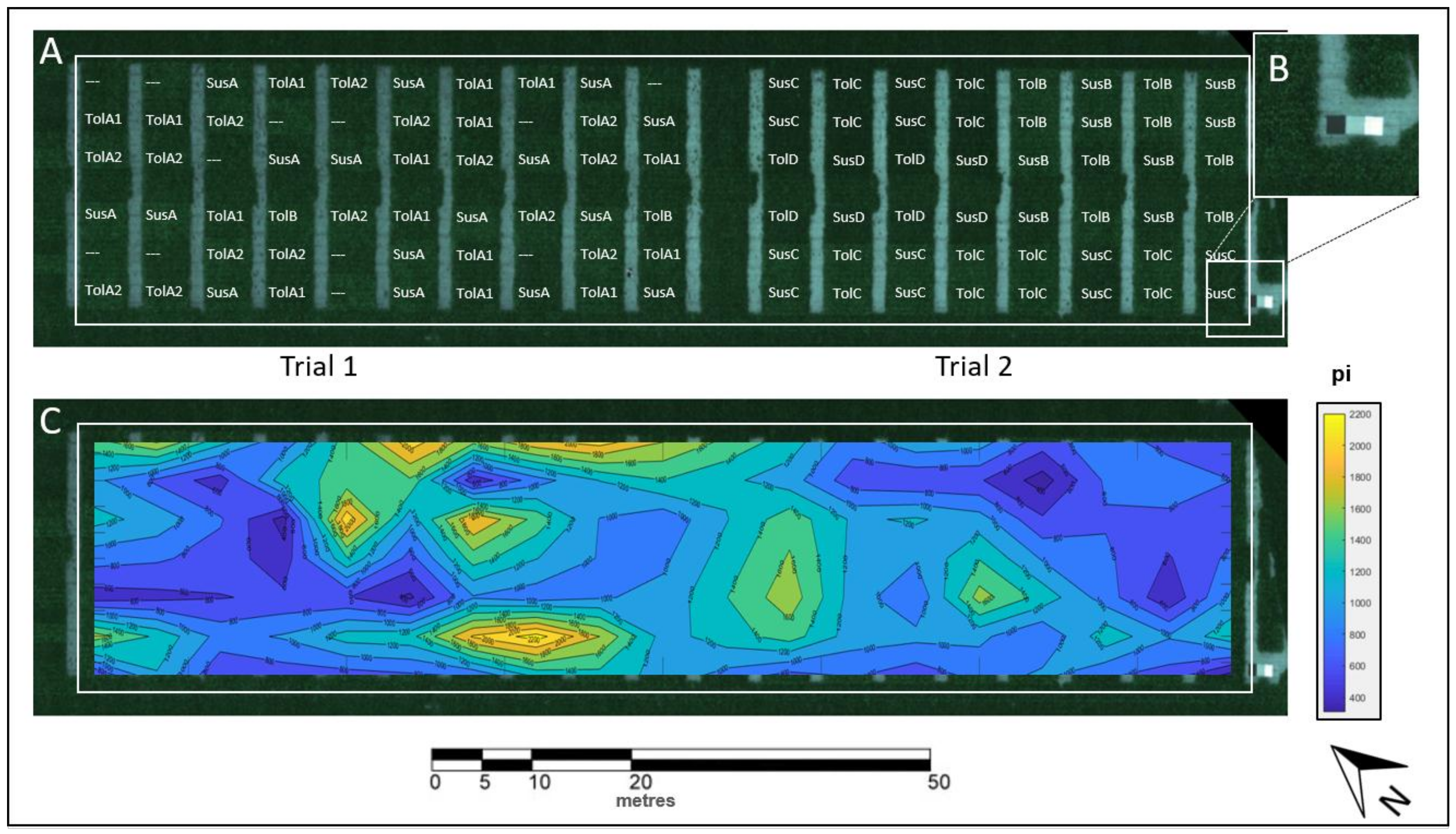
2.1. Experimental Site

Two sugar beet field trials were carried out side by side in 2016 in a field (0.4 ha) in Ober-Flörsheim (Rhineland-Palatinate, Germany) by the interest group for field experiments and extension in sugar beet (“Arbeitsgemeinschaft für Versuchswesen und Beratung im Zuckerrübenanbau Südwest“-ARGE Zuckerrübe Südwest). The site is located 49°68′N, 8°15′E at an altitude of 244 m above sea level. The field site was selected based on its natural infestation with BCN. The soil is a sandy loam (pH 7.5) containing 29.5 kg P2O5 ha−1, 45 kg K2O ha−1, 9.2 kg Mg ha−1. Fertilizer application followed best practice, with a base fertilizer application of 159 kg N ha−1, 54 kg P2O5 ha−1, 96 kg K2O ha−1 and 24 kg Mg ha−1 prior to sowing on 24 March.
Herbicide was applied during the first two months after sowing to avoid the influence of weeds on the plant growth (18 April: 1.2 L ha−1 Powertwin Plus + 1.5 L ha−1 Goltix, (Feinchemie Schwebda GmbH, Eschwege, Germany); 2 May: 1.25 L ha−1 Powertwin Plus + 1.5 L ha−1 Goltix; 7 May: 0.5 L ha−1 Gallant, (Dow Agrosciences, Indianapolis, USA); 17 May: 1.25 L ha−1 Powertwin Plus + 1.5 L ha−1 Goltix + 0.2 L ha−1 Tramat (Bayer Cropscience, Monheim, Germany). To control fungal pathogens one liter ha−1 Spyrale (Syngenta AG, Basel, Switzerland) was applied twice during the season, on 19 July and 18 August. This management reflects conventional intensive sugar beet cultivation in the region.
The climate of the study area is temperate with a mean annual rainfall of around 611 mm. From sowing on 24 March until harvest on 6 October, mean minimum and mean maximum temperatures were 10.1 °C and 21.0 °C, respectively.

2.2. Experimental Design

Two trials were established in two separate block designs (Table 1 and Figure 1) with the initial purpose of the trial to compare susceptible and tolerant cultivars from the same seed provider; plots were gathered at the same locations in order to minimize the variability in nematode pressure. No gradients in soil conditions were observed within the experimental field. Individual plots were three meters wide by eight meters long with a row distance of 0.5 m and a target sowing density of 11.1 seeds per m2. In trial 1, one susceptible and two tolerant cultivars were planted (Sus A, Tol A1, and Tol A2 from the breeder A). In trial 2, three susceptible and three tolerant cultivars were sown (Breeders B, C and D). In the present manuscript, A, B, C, and D are groups of cultivars corresponding to four different breeders (companies), supposedly reflecting different genetic backgrounds.
Sugar beet cultivars were randomized in a block design with 16 and eight replicates per treatment for experiments 1 and 2, respectively. Both trials were located in the same field.

2.3. Plant and Nematode Evaluation

The trials were harvested 196 days after sowing (das) on 6 October 2016. Three middle rows were harvested for each plot (17 m2). Final beet fresh weight and white sugar yield were determined for each single plot as described in Reuther et al. [40].
The initial BCN population density (pi) in the different plots was assessed at the time of planting and the final BCN population (pf) was assessed at harvest. Soil cores were sampled in each plot with a hydraulic soil sampler (Nietfeld, DUOPROB 60-UP, Quakenbrück, Germany). Ten samples were collected and automatically separated in topsoil (0–30 cm) and subsoil (30–60 cm) in the soil sampler. They were mixed to obtain one topsoil and one subsoil sample of minimum 500 g each per plot. Samples were stored in the dark at 4 °C before analysis. The nematode population was evaluated using a method described by Grosse et al. [41]. Based on the observation that 50% of the dormant nematodes hatched, the nematode infestation levels were determined by multiplying the observed infestation levels by a correction factor of two [42]. Infestation level was expressed as the number of juveniles (J2s) of H. schachtii per 100 g of soil.

2.4. In-Field Measurements

Canopy height measurements were performed manually in the field 102 das using a ruler. Two measurements were taken from the middle of two rows, respectively on the first third of each plot and subsequently averaged (CHruler).
Thermal images were acquired 152 das using an infrared camera (Testo 885, Testo Ltd., Alton, UK), having a Si sensor with 320 × 240 pixels covering a spectral range of 8–14 µm, and a sensor sensitivity of <30 mK at 30 °C. As in a previous study [13] the thermal device was calibrated prior to taking pictures by setting up the emissivity to 96% and the reflected temperature compensation parameter to the current air temperature [43]. One picture was taken from the same side of each plot with an angle of 45° at a height of 1.5 m above the ground. Canopy temperature (TC) was determined by combining both thermal and visible images generated by the thermal camera. Temperature fluctuation in the field was assessed by evaluating the naked soil temperature (TS) between rows with the thermal camera ten times during the measurements. On average, TS was 28.7 °C (± 0.4 °C) and relative humidity was 54% at the time of measurement. Because of the stable ambient temperature (fluctuating less than 1.5%) during measurements no normalization to ambient temperatures was applied.
Spectral measurements in the field were performed at das 88, 102 and 152 during the plant development using a non-imaging spectro-radiometer (ASD FieldSpec® 4, Analytic Spectral Devices, Boulder, CO, USA) with a spectral range of 350–2500 nm. Canopy spectra were acquired from nadir view of the plots at a height of 1 m above canopy with a 25° field of view. For each plot, five spectra were randomly taken at distinct positions consisting of five spectral samples and averaged. Instrument radiometric optimization and reflectance calibration were performed each time prior to spectral sampling in every third plot using a Zenith Polymer® (SphereOptics, Herrsching am Ammersee, Germany) 99% reflectance target as white reference.

UAV-Based Data Acquisition

Aerial image spectroscopy was acquired 102 and 152 das with a Gamaya OXI VNIR 40 camera system (Gamaya, SA, Lausanne, Switzerland) consisting of two individual cameras measuring 16 bands in the visible (VIS) and 25 bands in the near-infrared (NIR) range, respectively. The System was mounted on a Solo drone (3D Robotics, Inc., San Diego, USA). The camera system provides 40 spectral bands between 475 nm and 875 nm with a full width half maximum (FWHM) ranging from approximately 15 to 25 nm. It was equipped with 25 mm focal length optics. The images were captured from an altitude of 80 m with at least 75% overlap and 60% sidelap. VIS and NIR images were de-convolved with the Sprocket software provided by Gamaya, using the raw images and a camera specific calibration profile resulting in two megapixel images (2048 × 1088 pixels) for each camera. Both sets of images were processed in Agisoft Photoscan Professional (v. 1.26, Agisoft, LLC, St.Petersburg, Russia) resulting in a digital surface model (DSM) and an orthophoto for VIS and NIR, respectively. Geometrically correct overlay was facilitated using virtual markers such as distinctive field (stones, plot corners) or infrastructure (street breaks or gully covers) features.
Reflectance computation was also done with the Sprocket software from Gamaya and the final hypercube was exported as a band interleaved by line (bil) format. Three targets of different reflectance were placed in the field, measured with the ASD spectro-radiometer and selected in the hypercube (Figure 1). The radiance spectra of those targets, as seen by the hyperspectral camera, are then used to estimate the most likely sunlight spectrum, which is assumed constant throughout the data acquisition. The sunlight spectrum can be estimated for each target, by dividing for each band the target's radiance from the camera by its known reflectance measured in the field. As three different targets were used, the three sunlight estimations were fused into the most likely one through the least square regression function in the sprocket software.
Regions of interest (ROI) reflecting individual plots were manually identified on the hyperspectral images using the ENVI software (v. 5.1, Harris Corporation, Melbourne, FL, USA). For each ROI, the average spectrum was extracted. At 102 and 152 das, canopy height measurements were extracted from the DSM computed from the hyperspectral drone images (CHDSM). CHDSM for each plot was calculated as the difference between the average canopy elevation extracted from a ROI on the first third of the plot (1.8 m2, 3500 pixels ± 500) and the average soil elevation extracted in front of each plot (1.8 m2, 3500 pixels ± 500), respectively.
For each date of measurement and each plot, 123 published SIs were computed using the field spectrometer measurements. Seventy-seven SIs (reduced spectral range) were calculated from the hyperspectral images using the closest available channels for the SI calculation. The number of SIs was reduced subsequently for both spectral devices using a correlation matrix as described by Joalland et al. [13] to a small number of SIs, reflecting a range of traits, selected for further analysis (Table 2). In brief, SIs highly inter-correlated to each other (Pearson’s correlation coefficient p > 0.8) were grouped. One SI was then selected for each group. Selected SIs reflect the broad range of traits for which the SIs were initially developed.

2.5. Statistical Data Analysis

Data were analyzed with the statistical program R [54]. Beet fresh weight, white sugar yield and BCN population were exposed to analysis of variance (ANOVA) at a significance level of 0.05. ANOVA was used to compare and differentiate the cultivars for the computed or measured traits. PCA (Principal component analysis) was performed using the main selected phenotyping parameters computed from the infield measurements (thermal images and field spectrometer) and the UAV hyperspectral imager respectively.
To build decision trees we used the WEKA software (The Waikato Environment for Knowledge Analysis v. 3.8, 2016) and the J48 algorithm [55]. The decision trees were calibrated and cross-validated using an n-fold approach with n = 10 [56]. This cross-validation is considered as a conservative estimation of model accuracy. The total dataset was partitioned into 10 groups and 10 new subsets of the total were created using nine out of the 10. Ten test trees were then built using the reduced datasets; the unused 10% in each case was used to compute the classification error for each tree. Once the 10 test trees were built, their classification error rate as a function of tree size was averaged. Finally, the reference tree was pruned to the number of nodes matching the size that produced the minimum cross validation cost [57]. The decision trees were built for two sets of data: (1) Ground phenotyping (123 SIs, TC and CHruler) and (2) UAV derived parameters (77 SIs, CHDSM) at 102 and 152 das.

3. Results

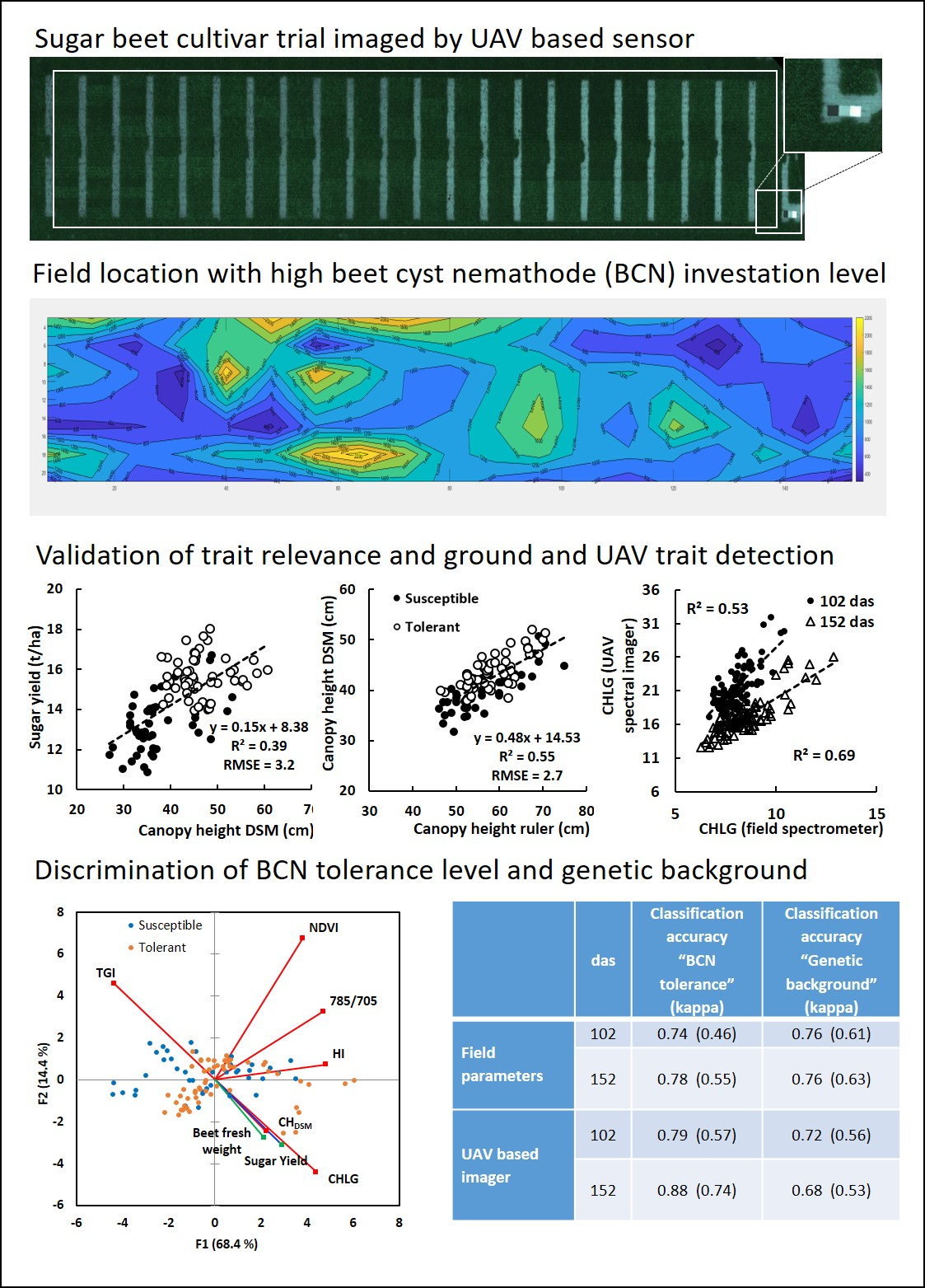
3.1. Spatial BCN Distribution in the Field

The spatial distribution of the initial BCN population density varied strongly throughout the experimental field (Figure 1). At sowing, BCN population densities ranged from 306 to 2284 J2s per 100 g of the topsoil and from 320 to 3457 J2s per 100 g in the subsoil. Overall, BCN population distribution was relatively even and high, with 90% of the plots infested with more than 600 J2s per 100 g of soil (Figure 1c).
The initial BCN population density per treatment (cultivar) varied from 814 to 1283 J2s per 100 g soil on average in the topsoil (CV of 15%) (Table 3). There was no significant difference between the initial BCN infestations of the treatments, which were all affected by a high BCN pressure on average. The ratio pf/pi is an indicator for reproduction and represents the ability of the cultivar to prevent nematode reproduction in the roots [58]. The reproduction index pf/pi in the topsoil was on average 1.1 for the tolerant cultivars and 8.6 for the susceptible cultivars (Figure 2). Tolerant cultivars B and D performed the best with an average pf/pi ratio below one (0.65 and 0.55, respectively).

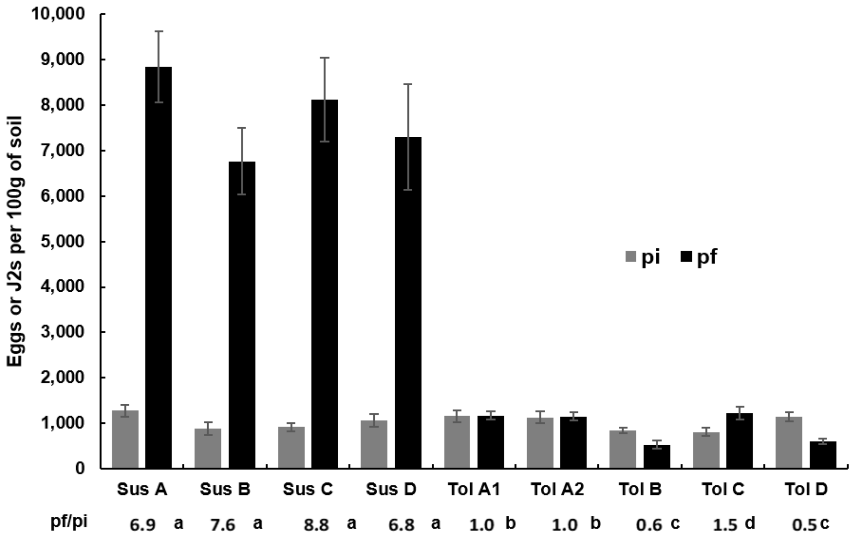
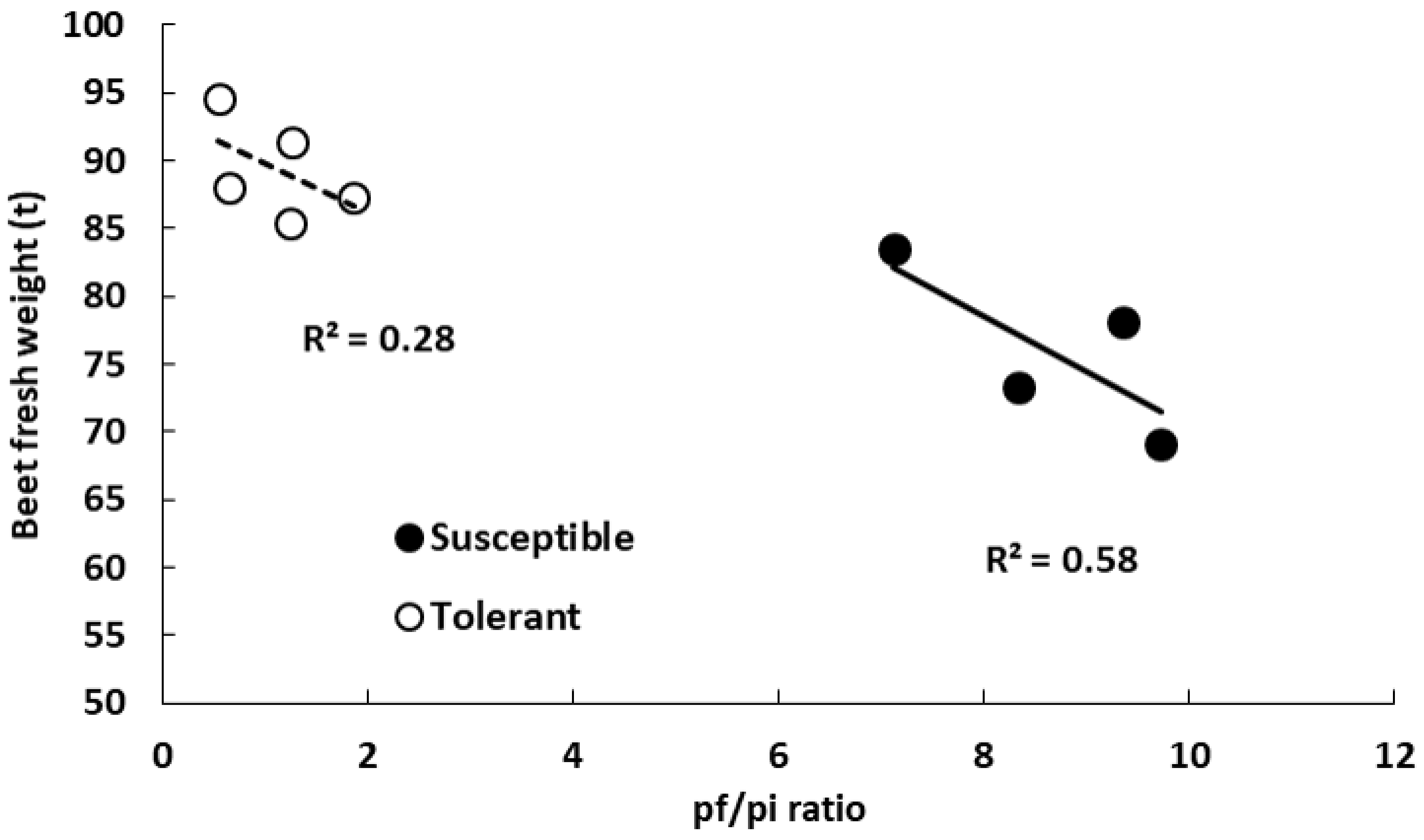
3.2. Beet Fresh Weight and Nematode Population

The tolerant cultivars produced higher beet fresh weight (BFW) than the susceptible cultivars. The highest white sugar yield (WSY) of 17.17 t ha−1 was observed for the tolerant cultivar D. On average, BFW and WSY were significantly higher for the tolerant cultivars compared to the susceptible ones (on average +18% and +17%, respectively). There was no significant correlation between the initial BCN population density and the yield of the different cultivars. Thus, we assume yield differences between cultivars were not caused by differences in initial BCN population density but by differences in the cultivar response to nematodes.
For both susceptible and tolerant cultivars, final beet fresh weight was not significantly correlated with the pf/pi ratio (Figure 3). However, there was a trend showing that the more nematodes reproduce in the roots, the higher is the yield-reducing effect. This trend was higher for the susceptible cultivars (R2 = 0.58, p = 0.24) than for the tolerant ones (R2 = 0.28, p = 0.37).

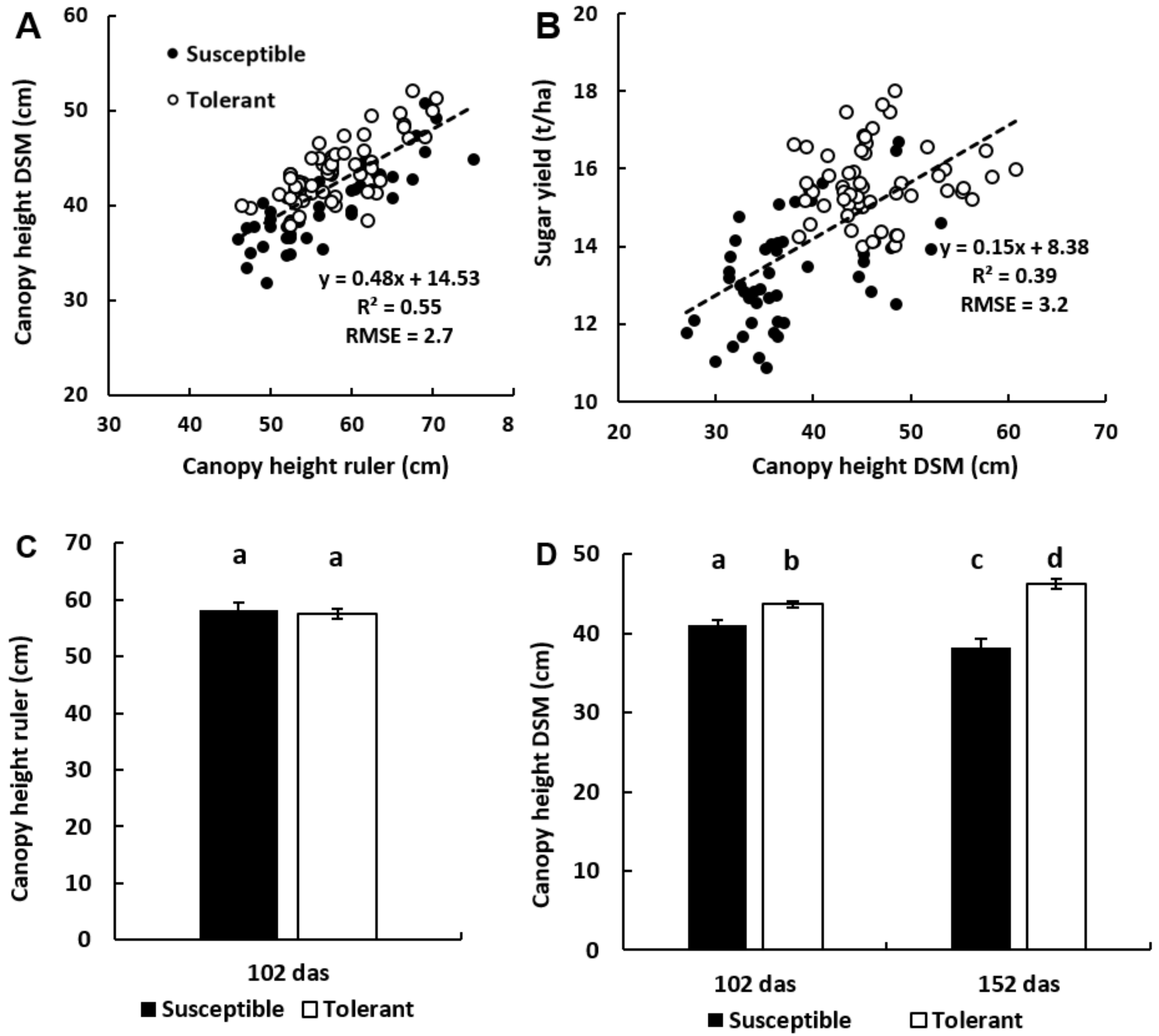
3.3. Canopy Height Measurements
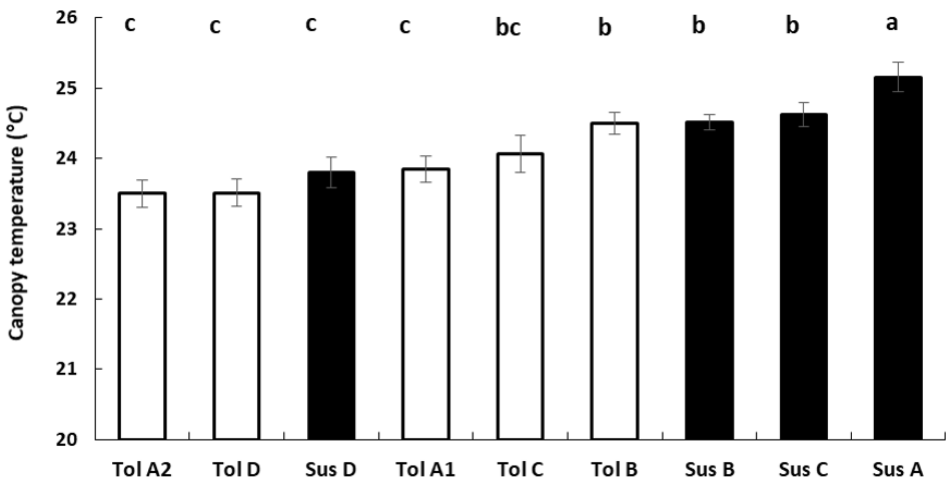
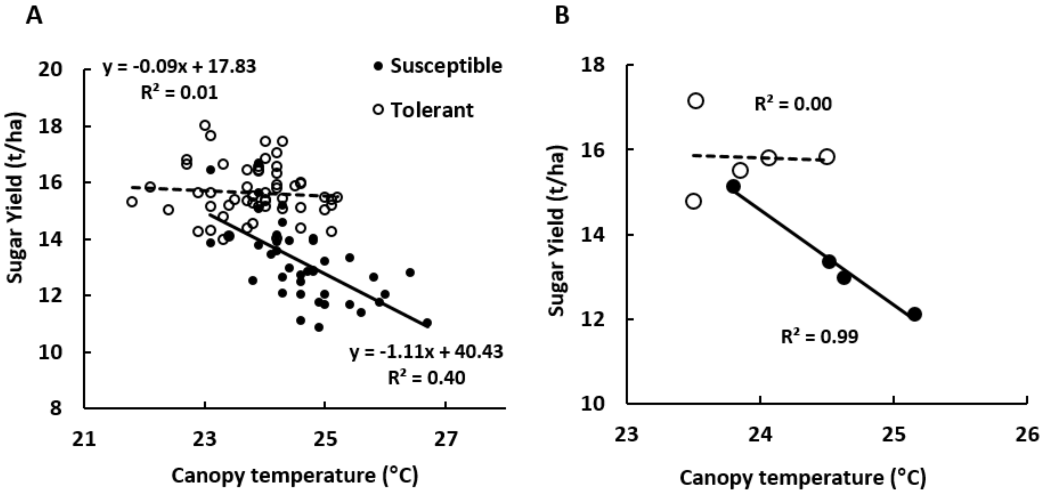
CHDSM and CHruler showed a good correlation 102 das (R2 = 0.55, p < 0.01) demonstrating that the DSM derived from a UAV platform is a valuable source to evaluate the canopy height (Figure 4a). The error on the canopy height evaluation was less than 3 cm. The DSM tends to underestimate the CHruler by 14.5 cm measured in the middle of rows. However, the amount of CHruler measurements was limited in number due to the need for physically entering the field and plot. The relatively high underestimation is likely caused by the selective use of the middle row height only for CHruler, being higher than the average plot height reflected by CHDSM because inter-row height were not measured on the ground. Nevertheless, CHruler reflects a genotype specific height measure sufficient to differentiate tolerant and susceptible genotypes. Therefore, we consider CHDSM as equivalent or even better.
Sugar yield prediction power using CHDSM extracted 152 das was weak but significant (R2 = 0.39, p < 0.01).
However, CHDSM of the tolerant cultivars was significantly higher than the CHDSM of the susceptible ones at the two dates of measurements (Figure 4d), which was not the case for CHruler, where no significant differences were observed between the two types of cultivars 102 das (Figure 4c). Interestingly, CHDSM of susceptible cultivars was significantly lower by 1.4 cm at the measurement on 152 das, while CHDSM of the tolerant cultivars significantly increased by 3.6 cm during the same time.

3.4. Thermography

Canopy temperature (TC) allowed us to rank cultivars according to their ability to cool down under moderate environmental stress (TAIR 28.7 °C, RH 54%). Average TC of the susceptible cultivars was significantly higher than TC of the tolerant ones (24.7 °C ± 0.1 vs. 23.8 ± 0.1 on average). The average cooling effect of the tolerant cultivars was 5.4% higher than that of the susceptible cultivars (data not shown). Three susceptible cultivars displayed the highest TC (Figure 5). Susceptible cultivar D displayed a TC similar to the tolerant cultivars.
Relationships between TC and sugar yield are presented at the plot and cultivar levels in Figure 6. At the plot level, high correlations could be observed between the canopy temperature and the white sugar yield for the susceptible cultivars (R2 = 0.40, p < 0.01). The correlation was very high at the cultivar level for the susceptible cultivars (R2 = 0.99, p < 0.01). In contrast, no correlation between TC and final yield could be observed for the tolerant cultivars.

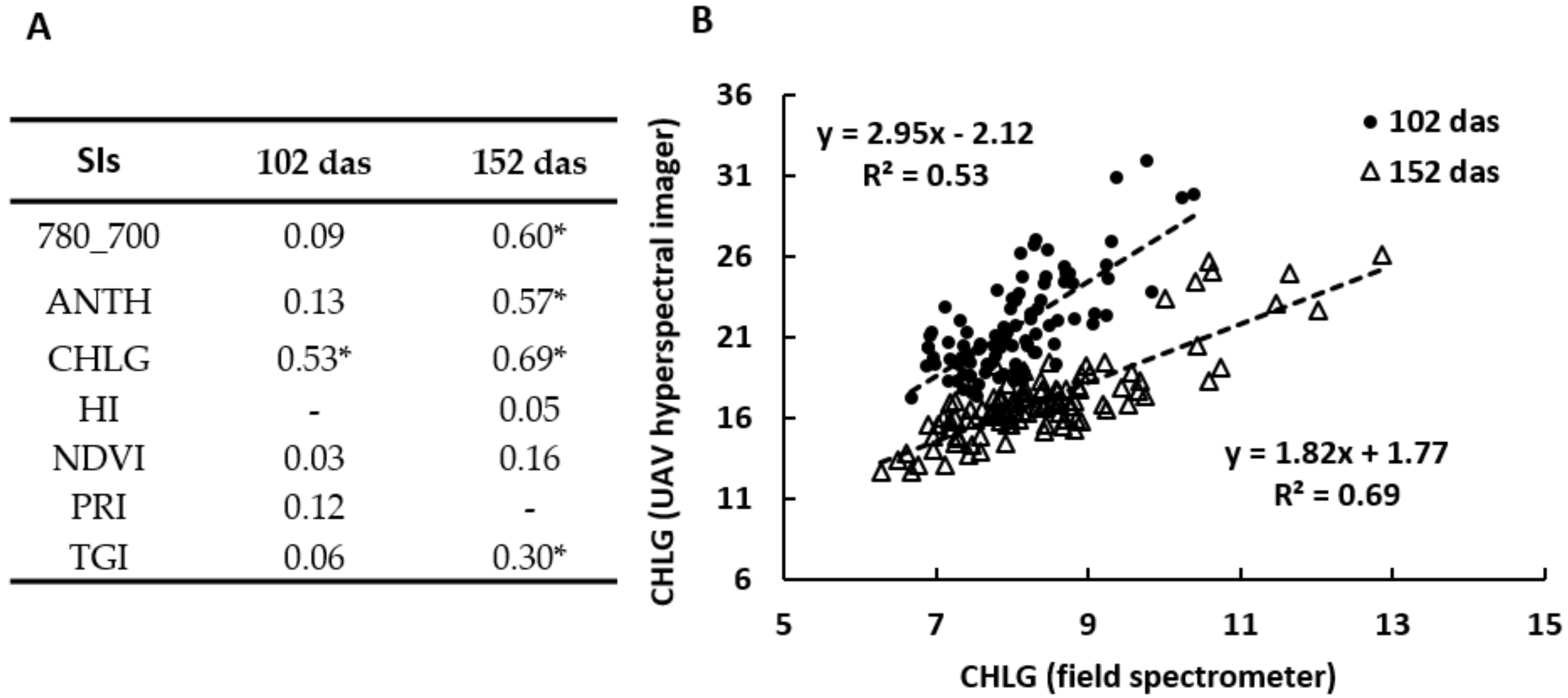
3.5. Spectrometry and UAV Hyperspectral Imaging

3.5.1. Discrimination of Susceptible and Tolerant Cultivars

We found several SIs suitable for discriminating susceptible and tolerant cultivars of each group for both field spectroscopy and UAV hyperspectral imaging (Table 4). The selected SIs reflect plant traits such as leaf chlorophyll and water content, leaf area index, and biomass which are expected to be affected by severe BCN infestation. Surprisingly, it was not possible to find SIs to significantly discriminate susceptible and tolerant cultivars at 88 das; this was likely related to the subtle or small differences related to the small plant size in early growth stages. For later stages, the SIs HI, CHLG or 780/700 were particularly suitable for differentiating susceptible and tolerant cultivars over two dates of measurements and three different cultivars. After 102 days, the main differences between susceptible and tolerant cultivars were related to biomass (NDVI), chlorophyll content of the leaves (780/700, CHLG) and general stress (HI). At 152 das, susceptible cultivars could also be differentiated from the tolerant ones using the SIs related to water content (NDWI1650, NDWI). The range of the hyperspectral imager on the UAV did not include short wave infrared bands, which prevented the calculation of spectral indices related to the water absorption bands. SIs extracted from the UAV hyperspectral device were not able to differentiate between the two types of cultivars from group C.

3.5.2. Correlations with the Yield in Susceptible and Tolerant Cultivars

Best correlations between SIs and the final sugar yield were obtained for susceptible cultivars (Table 5). Correlations were higher using SIs from the field spectrometer than from the hyperspectral imager. For the imager, significant correlations to sugar yield were only found after 102 days. Already after 88 days, SIs related to chlorophyll content (780/700, CHLG) or water content (NDWI1650, WI) allowed to predict the final sugar yield for the susceptible cultivars (Table 5). Correlations between SIs and final yield were lower for the tolerant cultivars at the two first dates of measurements. 152 das prediction of yield was good for both types of cultivars.

3.5.3. Field Spectrometer versus UAV Hyperspectral Imager

Good correlations were observed for the determination of the CHLG index between both spectrometers at the two dates of measurements (Figure 7). Other indices related to chlorophyll (780/700, ANTH) or photosynthesis (TGI) were well correlated after 152 das. The two methods differed significantly in terms of the values of HI. At 102 das, values of most of the indices were not consistent between both sensors.

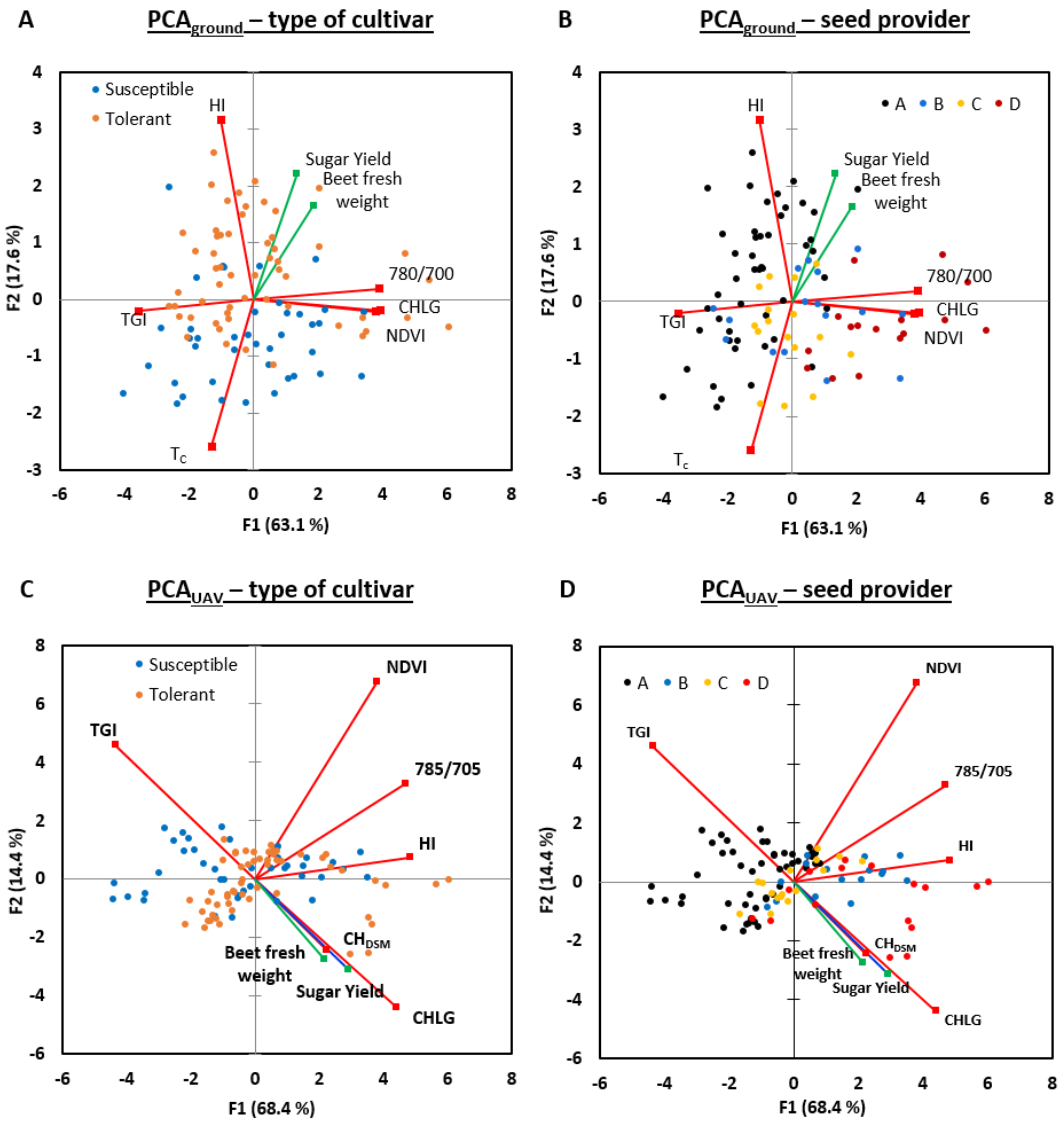
3.6. Multivariate Analysis

Studying single parameters allowed to differentiate between susceptible and tolerant cultivars from the same group and to predict yield with a fairly good accuracy. Multivariate analysis allowed us to go further and discriminate between the type of cultivars independently from the group.
Two PCA were performed separately using ground data (PCAground) and UAV data (PCAUAV) on the third date of measurements 152 das (Figure 8). Sugar yield and beet fresh weight were used as explanatory variables. In the PCAground, 81% of the variance is explained by the two first principal components (Figure 8a,b). Results confirmed that high canopy temperature is correlated to yield reduction. Canopy temperature and HI appeared particularly suitable for differentiating susceptible and tolerant cultivars (Figure 8a). Cultivars from breeder A and D could be easily discriminated using indices related to chlorophyll (CHLG, 780/700, TGI) and biomass (NDVI) (Figure 8b). Cultivars from the two other companies showed a similar profile in terms of canopy reflectance. Overall, principal component F2 represents the ability of the sugar beets to tolerate nematodes while principal component F1 seems more related to the genetic background of the plants.
The differences observed between PCAground and PCAUAV confirms the low correlations between SIs computed from the field spectrometer and from the UAV hyperspectral imager. Variables used did not allow us to discriminate easily between the types of cultivars (Figure 8c). One reason is surely the missing thermal data at the UAV level. Another reason is that height measurements at ground level were not sufficient to reveal genotypic differences between the investigated sugar beet types, which in contrast UAV-based height measurements could show on plot level. PCAUAV confirmed the close relationship between canopy height and sugar yield at this advanced stage of the sugar beet growth. Cultivars from groups A and D could be differentiated using CHLG and TGI indices confirming the good ability of chlorophyll related indices for the characterization of genetic background.

3.7. Decision Trees

The univariate decision trees (UDT) were used to classify sugar beet according to the type of cultivar (susceptible or tolerant) or the genetic background (breeder) using multiple traits. The cross validation produced accurate results without an independent dataset for assessing the accuracy of the model [59]. We found that decision trees could classify cultivar type and genetic background using just a few parameters (Table 6). Model accuracy was very similar using parameters evaluated at the ground level and information sensed with the UAV hyperspectral imager. Average cultivar classification accuracy was 77% and 83% on 102 and 152 das, respectively. Classification of plots was slightly higher for the type of cultivars compared to the genetic background of the cultivars. Overall coefficients of agreement were good. The Kappa coefficient varied from 0.46, which can be considered as a “moderate” agreement to 0.74, which corresponds to a “substantial” agreement [60].
Interestingly the best classification between tolerant or susceptible cultivars was obtained 152 das using the UAV information with 88%. The UDT using UAV based data for the classification of susceptible or tolerant cultivars used the CHDSM as a main parameter for classification. This was not the case for the classification according to the genetic background. Overall, information related to vegetation density, height, water content and pigment content in the leaves were suitable for cultivar type classification (see the Supplementary Materials). Physiological information related to photosynthesis, canopy temperature, nitrogen content and water content were selected in the UDT to differentiate genetic backgrounds.

4. Discussion

The results of this study demonstrated that ground-based and airborne phenotyping methods including imaging, spectrometry and thermometry can be used in the field to evaluate the level of beet cyst nematode (BCN) tolerance of sugar beet cultivars and predict sugar yield.
Infestation levels observed in this field study can be considered as moderate to high. The tolerance limit, which is the nematode population below which no damage is detectable, could not be precisely evaluated in this study. However, it is estimated to be between 300 and 1000 J2s per 100 g of soil for the nine cultivars according to the field location and soil temperatures observed during the season [61,62]. Under such nematode stress, it was possible to rank cultivars according to their ability to withstand or recover from the nematode attack and yield well. As expected, the five cultivars described as tolerant showed higher yield than the ones known to be susceptible [63]. The high nematode multiplication rate observed in the four susceptible cultivars is aligned with the lower yield observed for these cultivars. Interestingly, two tolerant cultivars (B and D) presented a multiplication rate below one, indicating them as resistant since they decreased the nematode population in the field [40,64]. Cultivar D combines high tolerance (high yield under nematode infestation) and high resistance (prevention of nematode multiplication), which is of advantage for use in infested fields. No significant correlation could be found between the initial number of BCN and the final yield. This was also shown by Reuther et al. [40] and may possibly be explained by the range of initial BCN population in the field, which was above the damage threshold.
Canopy height extracted from the DSM allowed us to differentiate between susceptible and tolerant cultivars which was not the case for the manual measurements CHruler. Since CHDSM takes approximately 3500 pixels representing single height estimates it can be assumed that the derived average canopy height is more realistic compared to the too few ground measurements per plot. This clearly shows a benefit of UAV-based imaging evaluation of traits such as canopy height that require lots of time and effort for manual evaluation in the field. The higher CHDSM differences between susceptible and tolerant cultivars observed 152 das can be explained by the higher nematode effect on susceptible cultivars, which increased over the season in contrast to the tolerant ones. However, DSM estimates can likely be improved with a higher overlap of images and crosswise flight paths and eventually a lower flying altitude. Additionally, stationary markers as used in [35] for geo-localization will further improve UAV-based height measurements. Such markers will also facilitate automated feature extraction based on geo-coordinates and thus reduce data extraction time.
The canopy temperature (TC) showed high potential for classifying cultivars according to their susceptibility or tolerance to nematodes. Three out of four susceptible cultivars had the highest TC, reflecting the lower ability of these plants to transpire water and thus cool down. TC is closely correlated with the prevailing temperature of the local environment, the leaf transpiration rate and the stomatal conductance [30,42,65,66]. BCN damage in the roots decreases water uptake, which subsequently reduces the leaf transpiration rate and results in a higher TC [67,68,69]. The high correlation observed between TC and final sugar yield for the susceptible cultivars likely reflects the nematode damage effect. The higher the BCN damage on the roots is, the higher is the TC. Schmitz et al. [20] and Joalland et al. [13] had similar results for susceptible cultivars under field and semi-field conditions, respectively. That no correlation was observed for tolerant cultivars is likely related to the less affected water uptake and transpiration rate compared to those of susceptible cultivars [70,71,72]. Thus, TC is suitable to determine the level of susceptibility but less for determination of tolerance level or to predict final yield.
SIs were found to be useful indicators for quantitative and qualitative evaluation of the sugar beet canopy. Under moderate to high BCN infestation, single SIs related to chlorophyll content (CHLG), photosynthetic activity (PRI), plant biomass (NDVI) or general stress (HI) were able to discriminate tolerant and susceptible cultivars from the same breeder (same genetic background). This is in line with many studies using spectroscopy methods to investigate genotype trials or plant stress detection [11,19,27,53]. Thus, for crop improvement studies or other experimental trials, spectrometry and/or spectral imaging is a fast and reliable screening method to characterize and rank different cultivars from the same genetic background according to their reaction to treatments or stresses. Here, we were able to demonstrate this for sugar beet cultivars and for their ability to tolerate nematodes. Yet, when the genetic background between cultivars differed widely (namely between cultivars from different seed companies), it was not possible to use a single SI to robustly discriminate the tolerant and susceptible cultivars. Here, the use of several relatively independent SIs was needed to identify the type of cultivars under BCN infestation. Combining SIs and thermal information integrates various aspects of plant growth and development such as canopy structure, biomass, pigment and water content, and photosynthetic activity, so such a combination can be a powerful tool to classify cultivars, even in experiments incorporating high genetic diversity.
In this study we combined the various measured parameters by using decision trees. After 152 days, CHDSM, chlorophyll- and water-content-related SIs were essential for discrimination between susceptible and tolerant cultivars, which demonstrates the high diversity and non-specificity of nematode-caused symptoms [6].
Interestingly, cultivars from group A and group D could be classified with high accuracy. This is clearly reflected in the PCA where plots from both groups were separately clustered. Such results illustrate the high variability caused by the intrinsic genetic background of each breeder, which is reflected in the plant physiology (water content, pigment concentration, photosynthetic activity) and plant performance (CHDSM, biomass). Cultivars that were bred using different germplasm pools may display very different reflectance spectra although depicting a similar tolerance level. While CHDSM appeared as an important parameter for the cultivar type classification, it was not useful for classification of the breeder.
SIs related to leaf chlorophyll showed high correlations with the final sugar yield for all ground and aerial measurements for the susceptible cultivars. This observation is consistent with the observation that more nematode damage on the roots triggers more visible symptoms on the shoots and thus causes yield reduction. As early as 88 das, SIs related to nitrogen status and water content such as 780/700 and NDWI, respectively could be used to predict yield with high precision. Hillnhütter et al. [19] also showed correlations between water content or leaf pigment related SIs and beet fresh weight in an infested field. However, yield prediction on tolerant cultivars was best after 152 days, when environmental conditions were more constraining (air temperature 28.7 °C, RH 54%) and likely the nematode stress affected the sugar beet growth for a longer period making differences more pronounced. Such moderate environmental stress as observed in this field study was obviously increased by the nematode stress and allowed to significantly differentiate tolerant cultivars and better predict final yield. Stronger symptoms were also observed on a tolerant cultivar under semi-field conditions when drought stress was higher [13].
The data obtained from the field spectrometer and the hyperspectral imager were not consistently correlated, which is also reflected by the differences observed between PCA computed with ground and UAV data. Such partly mismatch can be explained by differences between sensors and the measurement and calibration procedure. The instruments used have different sensor and filter technology causing different spectral resolution and spectral response, which causes the slightly altered shape of the derived spectra. The field spectrometer had a very high resolution, while the hyperspectral imager had a lower spectral resolution. As a consequence, some SIs, such as HI, were computed using slightly different bands, which resulted in low correlation between them [19]. In addition, the ground sampling resolution differed between the two measurement approaches. Whereas the average spectra per plot for the field spectrometer are the average of five point measurements with a footprint of about 50 cm diameter at random locations in each plot, the plot spectra obtained from the hyperspectral imaging were an average of thousands of pixels with an instantaneous field of view (ifov) of two cm. Further, the processing and calibration steps of both instruments differ. The field spectrometer is calibrated every 15 measurements (every three plots) using a white reference. The hyperspectral images are orthomosaicked using structure from motion procedures in Agisoft software before being calibrated to reflectance with a partial least squares regression using three reflectance panels differing in absolute reflectance intensity (Figure 1). Better understanding of the procedures in the sensors used and the consequences for the resulting measurements will surely improve the use of aerial imaging methods in the future. First attempts can be seen in the standardization of calibration methodology and cross validation [73].
Although SIs computed from the field spectrometer and from the spectral imager were not fully consistent, results and conclusions regarding the sugar beet phenotype were similar. Both tools were able to detect stress caused by nematodes and predict the final yield. This showed the great potential of UAV hyperspectral imagery to generate maps of nematode symptoms and yield potential of sugar beets with a high throughput. Such maps, combined with a reduced number of soil samples in the field to confirm the presence of nematodes, allow determination of spatial distribution and density of nematode infestation in agricultural fields. Such knowledge may help to select the right countermeasure such as optimized crop rotations or use of catch crops or appropriate tolerant sugar beet cultivars. For breeding purposes, such technology can make selection monitoring more efficient and thus accelerate crop improvement [74]. In our experimental field, tolerant and susceptible cultivars could be classified with an accuracy of over 80% on average. Specific SIs alone or combined and added to canopy height and temperature information have the ability to quantify traits related to BCN damage and to final sugar yield. Cultivar response to nematodes can be deduced in a fast and efficient manner and might be linked to physiological traits such as chlorophyll and water content, plant biomass or photosynthesis rate. Such a targeted analysis of traits will significantly improve the efficiency of sugar beet breeding for nematode tolerance and resistance.

5. Conclusions

Remote sensing methods were able to identify BCN symptoms on sugar beet plants and discriminate the type of cultivars under real field conditions. While thermography appeared suitable for yield prediction on susceptible cultivars only, field spectrometry and aerial UAV hyperspectral imaging were able to predict yield on susceptible and tolerant cultivars, likewise. Despite disparities in spectral and spatial resolution, both spectral tools can be used to characterize nematode symptoms and classify cultivars. Multivariate methods were precious tools to identify genetic backgrounds of the sugar beet cultivars and their ability to tolerate nematodes using a diversity of spectral indices. The UAV equipped with a hyperspectral imager proved to be a valuable tool for BCN stress diagnosis in the field and for improving breeding efficiency facilitating the monitoring of multiple traits at the same time and potentially at multiple sites. The most valuable remotely sensed traits to monitor for BCN tolerance and yield potential were canopy height, spectrally inferred chlorophyll content, leaf area or biomass, and canopy temperature.

Supplementary Materials

The following are available online at https://www.mdpi.com/2072-4292/10/5/787/s1, Table S1: Classification and mis-classification matrices for BCN tolerance type of cultivar using ground measurements and UAV hyperspectral data 102 and 152 das. (1) Ground-102 das; (2) Ground-152 das; (3) UAV-102 das; (4) UAV-152 das; Table S2: Classification and mis-classification matrix for genetic background (breeder) using ground measurements and UAV hyperspectral data 102 and 152 das. (1) Ground-102 das; (2) Ground-152 das; (3) UAV 102 das; (4) UAV 152 das; Table S3: Additional SIs selected by the UDT model to classify the types of cultivar and genetic background.

Author Contributions

M.R., M.S. and C.L. conceived and designed the trial. S.J. and F.L. planned and performed the remote sensing campaigns supported by C.S. and A.W. S.J., F.L. and H.V.V. analyzed the data and performed the statistical analysis. All authors contributed to writing and reviewing of the manuscript.

Acknowledgments

We are very grateful for the technical support of the “Arbeitsgemeinschaft für Versuchswesen und Beratung im Zuckerrübenanbau Südwest”-ARGE Zuckerrübe Südwest (Germany) in setting up the field trial. We also thank Marc Bonfils for leading the collaboration with Ruebe and making the phenotyping measurements possible. We also thank Lukas Roth for the great support in processing the hyperspectral UAV data, Norbert Kirchgessner for the contour map, and Verity Paul for her careful review of the manuscript and for her valuable suggestions and corrections.

Conflicts of Interest

The authors declare no conflict of interest.

References

  1. Food and Agriculture Organization (FAO). Global Agriculture towards 2050; Food and Agriculture Organization (FAO): Rome, Itlay, 2009. [Google Scholar]
  2. Müller, J. The economic importance of Heterodera schachtii in Europe. Helminthologia 1999, 36, 205–213. [Google Scholar]
  3. Biancardi, E.; McGrath, J.M.; Panella, L.W.; Lewellen, R.T.; Stevanato, P. Sugar beet. In Root and Tuber Crops; Springer: New York, NY, USA, 2010; pp. 173–219. [Google Scholar]
  4. Steele, A.E.; Arnold, E. The host range of the sugar beet nematode; Heterodera schachtii Schmidt. J. Am. Soc. Sugar Beet Technol. 1965, 13, 573–603. [Google Scholar] [CrossRef]
  5. Harveson, R.M.; Jackson, T.M. Sugar Beet Cyst Nematode; University of Nebraska–Lincoln Extension: Lincoln, NE, USA, 2008. [Google Scholar]
  6. Cooke, D.A. Beet cyst nematode (Heterodera schachtii Schmidt) and its control on sugar beet. Agric. Zool. Rev. 1987, 2, 135–183. [Google Scholar]
  7. Schmitz, A.; Tartachnyk, I.I.; Kiewnick, S.; Sikora, R.A.; Kühbauch, W. Detection of Heterodera schachtii infestation in sugar beet by means of laser-induced and pulse amplitude modulated chlorophyll fluorescence. Nematology 2006, 8, 273–286. [Google Scholar] [CrossRef]
  8. Heath, W.L.; Haydock, P.P.J.; Wilcox, A.; Evans, K. The potential use of spectral reflectance from the potato crop for remote sensing of infection by potato cyst nematodes. Asp. Appl. Biol. 2000, 60, 185–188. [Google Scholar]
  9. Nutter, F.W.; Tylka, G.L.; Guan, J.; Moreira, A.J.D.; Marett, C.C.; Rosburg, T.R. Use of remote sensing to detect soybean cyst nematode-induced plant stress. J. Nematol. 2002, 34, 222–231. [Google Scholar] [PubMed]
  10. Laudien, R. Entwicklung Eines GIS-Gestützten Schlagbezogenen Führungsinformationssystems für die Zuckerwirtschaft. (Development of a Field- and GIS-Based Management Information System for the Sugar Beet Industry). Ph.D. Thesis, University of Hohenheim, Stuttgart, Germany, 2005. [Google Scholar]
  11. Hillnhütter, C.; Mahlein, A.K.; Sikora, R.A.; Oerke, E.C. Use of imaging spectroscopy to discriminate symptoms caused by Heterodera schachtii and Rhizoctonia solani on sugar beet. Precis. Agric. 2012, 13, 17–32. [Google Scholar] [CrossRef]
  12. Joalland, S.; Screpanti, C.; Gaume, A.; Walter, A. Belowground biomass accumulation assessed by digital image based leaf area detection. Plant Soil. 2016, 398, 257–266. [Google Scholar] [CrossRef]
  13. Joalland, S.; Screpanti, C.; Liebisch, F.; Varella, H.V.; Gaume, A.; Walter, A. Comparison of visible imaging; thermography and spectrometry methods to evaluate the effect of Heterodera schachtii inoculation on sugar beets. Plant Methods 2017, 13, 73. [Google Scholar] [CrossRef] [PubMed]
  14. Sher-Kaul, S.; Oertli, B.; Castella, E.; Lachavanne, J.B. Relationship between biomass and surface area of six submerged aquatic plant species. Aquat. Bot. 1995, 51, 147–154. [Google Scholar] [CrossRef]
  15. Smith, S.M.; Garrett, P.B.; Leeds, J.A.; McCormick, P.V. Evaluation of digital photography for estimating live and dead aboveground biomass in monospecific macrophyte stands. Aquat. Bot. 2000, 67, 69–77. [Google Scholar] [CrossRef]
  16. Mizoue, N.; Masutani, T. Image analysis measure of crown condition; foliage biomass and stem growth relationships of Chamaecyparis obtusa. For. Ecol. Manag. 2003, 172, 79–88. [Google Scholar] [CrossRef]
  17. Tackenberg, O. A new method for non-destructive measurement of biomass; growth rates; vertical biomass distribution and dry matter content based on digital image analysis. Ann. Bot. Lond. 2007, 99, 777–783. [Google Scholar] [CrossRef] [PubMed]
  18. Baret, F.; Guyot, G. Potentials and limits of vegetation indices for LAI and APAR assessment. Remote Sens. Environ. 1991, 35, 161–173. [Google Scholar] [CrossRef]
  19. Hillnhütter, C.; Mahlein, A.K.; Sikora, R.A.; Oerke, E.C. Remote sensing to detect plant stress induced by Heterodera schachtii and Rhizoctonia solani in sugar beet fields. Field Crop Res. 2011, 122, 70–77. [Google Scholar] [CrossRef]
  20. Schmitz, A.; Kiewnick, S.; Schlang, J.; Sikora, R.A. Use of high resolution digital thermography to detect Heterodera schachtii infestation in sugar beets. Commun. Agric. Appl. Biol. Sci. 2004, 69, 359–363. [Google Scholar] [PubMed]
  21. Colomina, I.; Molina, P. Unmanned aerial systems for photogrammetry and remote sensing: A review. ISPRS J. Photogramm. Remote Sens. 2014, 92, 79–97. [Google Scholar] [CrossRef]
  22. Araus, J.L.; Cairns, J. Field high-throughput phenotyping—The new crop breeding frontier. Trends Plant Sci. 2014, 19, 52–61. [Google Scholar] [CrossRef] [PubMed]
  23. Walter, A.; Liebisch, F.; Hund, A. Plant phenotyping: From bean weighing to image analysis. Plant Methods 2015, 11, 14. [Google Scholar] [CrossRef] [PubMed]
  24. Bendig, J.; Bolten, A.; Bareth, G. Introducing a low-cost mini-UAV for thermal- and multispectral-imaging. In Proceedings of the XXII ISPRS Congress, Melbourne, Australia, 25 August–1 September 2012; pp. 345–349. [Google Scholar]
  25. Guo, T.; Kujirai, T.; Watanabe, T. Mapping crop status from an unmanned aerial vehicle for precision agriculture applications. In Proceedings of the XXII ISPRS Congress, Melbourne, Australia, 25 August–1 September 2012; pp. 485–490. [Google Scholar]
  26. Primicerio, J.; Di Gennaro, S.F.; Fiorillo, E.; Genesio, L.; Lugato, E.; Matese, A.; Vaccari, F.P.A. Flexible unmanned aerial vehicle for precision agriculture. Precis. Agric. 2012, 13, 517–523. [Google Scholar] [CrossRef]
  27. Tattaris, M.; Reynolds, M.P.; Chapman, S.C. A Direct Comparison of Remote Sensing Approaches for High-Throughput Phenotyping in Plant Breeding. Front. Plant Sci. 2016, 7, 1131. [Google Scholar] [CrossRef] [PubMed]
  28. Akhtman, Y.; Golubeva, E.; Tutubalina, O.; Zimin, M. Application of hyperspectral images and ground data for precision farming. Geogr. Environ. Sustain. 2017, 10, 117–128. [Google Scholar] [CrossRef]
  29. Constantin, D.; Rehak, M.; Akhtman, Y.; Liebisch, F. Detection of crop properties by means of hyperspectral remote sensing from a micro UAV. In Bornimer Agrartechnische Berichte; Leibniz-Institut für Agrartechnik Potsdam-Bornim eV: Potsdam, Germany, 2015; pp. 129–137. [Google Scholar]
  30. Khanna, R.; Möller, M.; Pfeifer, J.; Liebisch, F.; Walter, A.; Siegwart, R. Beyond point clouds-3d mapping and field parameter measurements using UAVs. In Proceedings of the IEEE 20th Conference on Emerging Technologies and Factory Automation (ETFA), Luxembourg, 8–11 September 2015; pp. 1–4. [Google Scholar]
  31. Liebisch, F.; Kirchgessner, N.; Schneider, D.; Walter, A.; Hund, A. Remote, aerial phenotyping of maize traits with a mobile multi-sensor approach. Plant Methods 2015, 11, 9. [Google Scholar] [CrossRef] [PubMed]
  32. Burkart, A.; Hecht, V.L.; Kraska, T.; Rascher, U. Phenological analysis of unmanned aerial vehicle based time series of barley imagery with high temporal resolution. Precis. Agric. 2018, 19, 134–146. [Google Scholar] [CrossRef]
  33. Jimenez-Bello, M.A.; Royuela, A.; Manzano, J.; Zarco-Tejada, P.J.; Intrigliolo, D. Assessment of drip irrigation sub-units using airborne thermal imagery acquired with an Unmanned Aerial Vehicle (UAV). In Precision Agriculture 13; Wageningen Academic Publishers: Wageningen, The Netherlands, 2013; pp. 705–711. [Google Scholar]
  34. Diaz-Varela, R.A.; de la Rosa, R.; Leon, L.; Zarco-Tejada, P.J. High-resolution airborne UAV imagery to assess olive tree crown parameters using 3D photo reconstruction: Application in breeding trials. Remote Sens. 2015, 7, 4213–4232. [Google Scholar] [CrossRef]
  35. Roth, L.; Streit, B. Predicting cover crop biomass by lightweight UAS-based RGB and NIR photography: An applied photogrammetric approach. Precis. Agric. 2017, 1–22. [Google Scholar] [CrossRef]
  36. Sankaran, S.; Khot, L.R.; Espinoza, C.Z.; Jarolmasjed, S.; Sathuvalli, V.R.; Vandemark, G.J.; Miklas, P.N.; Carter, A.H.; Pumphrey, M.O.; Knowles, N.R.; et al. Low-altitude; high-resolution aerial imaging systems for row and field crop phenotyping: A review. Eur. J. Agron. 2015, 70, 112–123. [Google Scholar] [CrossRef]
  37. Yang, G.; Liu, J.; Zhao, C.; Li, Z.; Huang, Y.; Yu, H.; Xu, B.; Yang, X.; Zhu, D.; Zhang, X.; Zhang, R.; et al. Unmanned Aerial Vehicle Remote Sensing for Field-Based Crop Phenotyping: Current Status and Perspectives. Front. Plant Sci. 2017, 8, 1111. [Google Scholar] [CrossRef] [PubMed]
  38. Yu, K.; Lenz-Wiedemann, V.; Chen, X.; Bareth, G. Estimating leaf chlorophyll of barley at different growth stages using spectral indices to reduce soil background and canopy structure effects. ISPRS J. Photogramm. 2014, 97, 58–77. [Google Scholar] [CrossRef]
  39. Sa, I.; Chen, Z.; Popovic, M.; Khanna, R.; Liebisch, F.; Nieto, J.; Siegwart, R. weedNet: Dense Semantic Weed Classification Using Multispectral Images and MAV for Smart Farming. IEEE Robot. Autom. Lett. 2018, 3, 588–595. [Google Scholar] [CrossRef]
  40. Reuther, M.; Lang, C.; Grundler, F.M.W. Nematode-tolerant sugar beet varieties—Resistant or susceptible to the Beet Cyst Nematode Heterodera schachtii? Sugar Ind. 2017, 142, 277–284. [Google Scholar]
  41. Grosse, E.; Banasiak, L.; Lyr, H.; Jock, M. Neuer Labortest zum Nachweis des Rübennematoden (Heterodera schachtii). Nachr.-Bl. Pflanzenschutz DDR 1985, 39, 111–112. [Google Scholar]
  42. Grosse, E.; Decker, H. Untersuchungen zur Eignung von Biotest und Schlupftest für den quantitativen Nachweis des Rübenzystenälchen (Heterodera schachtii) in Bodenproben. Nachr.-Bl. Pflanzenschutz DDR 1989, 43, 227–230. [Google Scholar]
  43. Oerke, E.C.; Steiner, U. Potential of digital thermography for disease control. In Precision Crop Protection—The Challenge and Use of Heterogeneity; Oerke, E.C., Gerhards, R., Menz, G., Sikora, R.A., Eds.; Springer: Dordrecht, The Netherlands, 2010; pp. 167–182. [Google Scholar]
  44. Rouse, J.W.; Haas, R.H.; Schell, J.A.; Deering, D.W. Monitoring Vegetation Systems in the Great Plains with ERTS; NASA: Goddard, MD, USA, 1974; Volume 351, p. 309. [Google Scholar]
  45. Mistele, B.; Gutser, R.; Schmidhalter, U.; Mulla, D.J. Validation of field-scaled spectral measurements of the nitrogen status in winter wheat. In Proceedings of the 7th International Conference on Precision Agriculture and Other Precision Resources Management, Hyatt Regency, Minneapolis, MN, USA, 25–28 July 2004; Precision Agriculture Center, Department of Soil, Water and Climate, University of Minnesota: Minneapolis, MN, USA, 2004; pp. 25–28, 1187–1195. [Google Scholar]
  46. Haboudane, D.; Miller, J.R.; Tremblay, N.; Zarco-Tejada, P.J.; Dextraze, L. Integrated narrow-band vegetation indices for prediction of crop chlorophyll content for application to precision agriculture. Remote Sens. Environ. 2002, 81, 416–426. [Google Scholar] [CrossRef]
  47. Hunt, E.R.; Daughtry, C.S.T.; Eitel, J.U.; Long, D.S. Remote sensing leaf chlorophyll content using a visible band index. Agron. J. 2011, 103, 1090–1099. [Google Scholar] [CrossRef]
  48. Gitelson, A.A.; Keydan, G.P.; Merzlyak, M.N. Three-band model for noninvasive estimation of chlorophyll; carotenoids; and anthocyanin contents in higher plant leaves. Geophys. Res. Lett. 2006, 33. [Google Scholar] [CrossRef]
  49. Gamon, J.A.; Penuelas, J.; Field, C.B. A narrow-waveband spectral index that tracks diurnal changes in photosynthetic efficiency. Remote Sens. Environ. 1992, 41, 35–44. [Google Scholar] [CrossRef]
  50. Gao, B.C. NDWI—A normalized difference water index for remote sensing of vegetation liquid water from space. Remote Sens. Environ. 1996, 58, 257–266. [Google Scholar] [CrossRef]
  51. Clay, D.E.; Kim, K.I.; Chang, J.; Clay, S.A.; Dalsted, K. Characterizing water and nitrogen stress in corn using remote sensing. Agron. J. 2006, 98, 579–587. [Google Scholar] [CrossRef]
  52. Penuelas, J.; Pinol, J.; Ogaya, R.; Filella, I. Estimation of plant water concentration by the reflectance water index WI (R900/R970). Int. J. Remote Sens. 1997, 18, 2869–2875. [Google Scholar] [CrossRef]
  53. Mahlein, A.K.; Rumpf, T.; Welke, P.; Dehne, H.W.; Plümer, L.; Steiner, U.; Oerke, E.C. Development of spectral indices for detecting and identifying plant diseases. Remote Sens. Environ. 2013, 128, 21–30. [Google Scholar] [CrossRef]
  54. R Development Core Team. R: A Language and Environment for Statistical Computing; R Foundation for Statistical Computing: Vienna, Austria, 2008. Available online: http://www.R-project.org (accessed on 1 July 2017).
  55. Witten, I.H.; Frank, E.; Hall, M.A.; Pal, C.J. Data Mining: Practical Machine Learning Tools and Techniques; Morgan Kaufmann: Burlington, MA, USA, 2016. [Google Scholar]
  56. Weiss, S.M.; Kulikowski, C.A. Computer Systems that Learn; Kaufmann Publishers: San Mateo, CA, USA, 1991. [Google Scholar]
  57. Breiman, L.; Friedman, J.; Olshen, R.; Stone, C. Classification and Regression Trees; Wadsworth International Group: Belmont, CA, USA, 1984. [Google Scholar]
  58. Oostenbrink, M. Major characteristics of the relations between nematodes and plants. In Proceedings of the 8th International Symposium of nematology, Antibes, France, 8–14 September 1966. [Google Scholar]
  59. Sherrod, P.H. DTREG Predictive Modeling Software. Users Manual. Available online: www.dtreg. com/DTREG.pdf (accessed on 1 February 2018).
  60. Landis, J.R.; Koch, G.G. The measurement of observer agreement for categorical data. Biometrics 1977, 33, 159–174. [Google Scholar] [CrossRef] [PubMed]
  61. Seinhorst, J.W. The relation between nematode density and damage to plants. Nematologica 1965, 11, 137–154. [Google Scholar] [CrossRef]
  62. Cooke, D.A.; Thomason, I.J. The relationship between population density of Heterodera schachtii; soil temperature; and sugarbeet yields. J. Nematol. 1979, 11, 124. [Google Scholar] [PubMed]
  63. Hauer, M.; Koch, H.J.; Märländer, B. Water use efficiency of sugar beet cultivars (Beta vulgaris L.) susceptible; tolerant or resistant to Heterodera schachtii (Schmidt) in environments with contrasting infestation levels. Field Crops Res. 2015, 183, 356–364. [Google Scholar] [CrossRef]
  64. Trudgill, D.L. Resistance to and tolerance of plant parasitic nematodes in plants. Annu. Rev. Phytopathol. 1991, 29, 167–192. [Google Scholar] [CrossRef]
  65. Inoue, Y.; Kimball, B.A.; Jackson, R.D.; Pinter, P.J.; Reginato, R.J. Remote estimation of leaf transpiration rate and stomatal resistance based on infrared thermometry. Agric. For. Meteorol. 1990, 51, 21–33. [Google Scholar] [CrossRef]
  66. Jones, H.G.; Schofield, P. Thermal and other remote sensing of plant stress. Gen. Appl. Plant Physiol. 2008, 34, 19–32. [Google Scholar]
  67. Trudgill, D.L. Effects of Globodera rostochiensis and fertilisers on the mineral nutrient content and yield of potato plants. Nematologica 1980, 26, 243–254. [Google Scholar] [CrossRef]
  68. Haverkort, A.J.; Fasan, T.; Van de Waart, M. The influence of cyst nematodes and drought on potato growth. 2. Effects on plant water relations under semi-controlled conditions. Eur. J. Plant Pathol. 1991, 97, 162–170. [Google Scholar] [CrossRef]
  69. Jones, H.G. Application of thermal imaging and infrared sensing in plant physiology and ecophysiology. Adv. Bot. Res. 2004, 41, 107–163. [Google Scholar]
  70. Evans, K.; Franco, J. Tolerance to cyst-nematode attack in commercial potato cultivars and some possible mechanisms for its operation. Nematologica 1979, 25, 153–162. [Google Scholar] [CrossRef]
  71. Trudgill, D.L. Concepts of resistance; tolerance and susceptibility in relation to cyst nematodes. In Cyst Nematodes; Springer: Boston, MA, USA, 1986; pp. 179–189. [Google Scholar]
  72. Radcliffe, D.E.; Hussey, R.S.; McClendon, R.W. Cyst nematode vs. tolerant and intolerant soybean cultivars. Agron. J. 1990, 82, 855–860. [Google Scholar] [CrossRef]
  73. Aasen, H.; Bolten, A. Multi-temporal high-resolution imaging spectroscopy with hyperspectral 2D imagers–From theory to application. Remote Sens. Environ. 2018, 205, 374–389. [Google Scholar] [CrossRef]
  74. Shakoor, N.; Lee, S.; Mockler, T.C. High throughput phenotyping to accelerate crop breeding and monitoring of diseases in the field. Curr. Opin. Plant Biol. 2017, 38, 184–192. [Google Scholar] [CrossRef] [PubMed]
Figure 1. Orthophoto of the experimental field extracted from the hyperspectral imager containing the experimental setup of the two investigated field trials (A); detail of the reflectance plates used for radiometric calibration as placed in the field (B); contour map of the initial BCN population density in the topsoil (0–30 cm) (C); The map was linearly interpolated from the 108 data points representing the sampled plots using the average of its neighbors for non-sampled plots.
Remotesensing 10 00787 g001
Figure 2. Average initial pi and pf BCN population in the soil for nine different cultivars. Error bars represent the standard error. Different letters behind pf/pi values indicate significant differences at p < 0.05.
Remotesensing 10 00787 g002
Figure 3. Beet fresh weight at harvest as a function of the nematode reproduction rate (pf/pi) in the soil for the four susceptible and five tolerant genotypes. Correlations were not significant.
Remotesensing 10 00787 g003
Figure 4. (A) Relationship between canopy height derived from the digital elevation model (CHDSM) and canopy measured by a ruler (CHruler) 102 das (n = 104, p < 0.01); (B) final sugar yield as a function of the CHDSM 152 das (n = 104, p < 0.01); (C) average CHruler of tolerant and susceptible cultivars 102 das; (D) average CHDSM of tolerant and susceptible cultivars 102 and 152 das. Error bars represent the standard error. Different lower case letters indicate significant differences between cultivar types at p < 0.05.
Remotesensing 10 00787 g004
Figure 5. Average canopy temperatures of five tolerant and four susceptible cultivars 153 das. Error bars represent the standard error. Different lower case letters indicate significant differences between genotypes (p < 0.05).
Remotesensing 10 00787 g005
Figure 6. White sugar yield at harvest as a function of the canopy temperature 152 das at the (A) plot and (B) cultivar levels.
Remotesensing 10 00787 g006
Figure 7. (A) Coefficient of determination R2 for the relationship between SIs computed from the field spectrometer and from the UAV hyperspectral imager. * Significant correlations (n = 96, p < 0.05); (B) relationship between CHLG index computed from field spectrometer and UAV hyperspectral imager at 102 (p < 0.01) and 152 das (p < 0.01).
Remotesensing 10 00787 g007
Figure 8. Principal component analysis (PCA) of the main phenotyping parameters 152 das. The percentage of variance explained by each component is displayed in parentheses. (A,B) display PCA using ground data (main field spectrometer SIs and canopy temperature); (C,D) show PCA using main SIs and canopy height extracted from the UAV. The susceptible and tolerant cultivars are depicted in blue and orange, respectively in graphs (A,C). The genetic background (breeder) are shown in different colors (graphs (B,D). Each data point represents one field plot (n = 96).
Remotesensing 10 00787 g008
Table 1. Summary of the experimental settings and the crop management operations during the two field trials.
Sugar beet cultivarsSusceptibleTolerant
Sus ATol A1
Tol A2
Sus BTol B
Sus CTol C
Sus DTol D
Sowing24 March 2016
Fertilizer applicationMid-March
Herbicide applications18 April
2 May
7 May
17 May
Fungicide application19 July
18 August
Ground measurementsSpectrometry20 June (88 das *)
4 July (102 das)
23 August (152 das)
Canopy height4 July (102 das)
Thermography23 August (152 das)
UAV Hyperspectral images acquisition4 July (102 das)
23 August (152 das)
Harvest and sampling6 October
* Days after sowing.
Table 2. Selected SIs, their respective equations (field spectrometer), the proposed detection trait and references.
SIsEquationTraitsReference
NDVI(R800 − R680)/(R800 + R680)Biomass, coverage[44]
780/740R780/R740Nitrogen content[45]
780/700R780/R700Nitrogen content[45]
TCARI3 × [(R700 − R670) − 0.2 × (R700 − R550) × (R700/R670)]Chlorophyll content[46]
TGI−0.5×[(W670 − W480)×(R670 − R550) − (W670 − W550)×(R670 − R480)]Chlorophyll content[47]
ANTHR760 − R800 × (1/R540 − R560 − 1/R690 − R710)Anthocyanins[48]
CHLG(R760 − R800)/(R540 − R560)Chlorophyll content[48]
PRI(R531 − R570)/(R531 + R570)Stress[49]
NDWI(R860 − R1240)/(R860 + R1240)Plant water status[50]
NDWI1650(R840 − R1650)/(R840 + R1650)Plant water status[51]
WI(R900/R970)Plant water status[52]
HI(R534 − R698)/(R534 + R698) − R704/2Plant health[53]
Table 3. Beet fresh weigh, white sugar yield and initial BCN population density of each sugar beet cultivar. Displayed, are the mean ± standard error of each treatment. Different lower case letters within each column indicate significant differences between genotypes (p < 0.05).
Cultivar TypeGenotypeBeet Fresh Weight (t)White Sugar Yield (t)Initial BCN Population (Number of J2s per 100 g soil)
Susceptible Susceptible A73.27 ± 1.39 a12.13 ± 0.23 a1283 ± 131 a
Susceptible B78.08 ± 2.30 a13.63 ± 0.44 b886 ± 144 a
Susceptible C69.10 ± 1.18 c13.00 ± 0.22 b919 ± 94 a
Susceptible D83.56 ± 2.05 d15.14 ± 0.38 cd1073 ± 140 a
Average 76.00 ± 1.0913.48 ± 0.221031
TolerantTolerant A191.41 ± 1.01 bf15.52 ± 0.17 c1160 ± 126 a
Tolerant A285.48 ± 0.97 d14.80 ± 0.14 d1134 ± 128 a
Tolerant B87.99 ±1.53 ef15.60 ± 0.30 c1512 ± 62 a
Tolerant C87.30 ± 0.80 de15.81 ± 0.22 c814 ± 90 a
Tolerant D94.66 ± 1.13 b17.17 ± 0.19 e1154 ± 103 a
Average89.37 ± 0.6315.78 ± 0.131026
Table 4. SIs that allow statistical discrimination of susceptible and tolerant cultivars in each group (p < 0.05). (A) Field spectrometer; (B) UAV hyperspectral imager. SIs common to both tools are highlighted in bold.
(A)Experiment 1Experiment 2
Sus A/Tol A1–Tol A2Sus B/Tol BSus C/Tol CSus D/Tol D
88 das
102 das780/700
HI
CHLG
PRI
NDVI
780/700
CHLG
HI
PRI
TGI
ANTH
HI
NDWI1650
NDWI
HI
152 das780/700
HI
TGI
PRI
CHLG
TCARI
NDWI1650
CHLG
NDWI
NDWI1650
PRI
TCARI
TGI
ANTH
HI
NDWI1650
780/700
ANTH
CHLG
NDVI
NDWI
NDWI1650
(B)Experiment 1Experiment 2
Sus A/Tol A1–Tol A2Sus B/Tol BSus C/Tol CSus D/Tol D
102 dasCHLG
HI
ANTH
PRI
CHLG
ANTH
PRI
CHLG
HI
ANTH
PRI
152 dasCHLG
ANTH
TGI
HI
785/705
NDVI
CHLG
ANTH
HI
CHLG
ANTH
TGI
HI
785/705
Table 5. Coefficient of determination R2 for the relationship between SIs and white sugar yield for susceptible and tolerant cultivars at different measurement times. (A) Field spectrometer; (B) UAV hyperspectral imager. * indicates significant correlations (n = 56 for the susceptible and n = 40 for the tolerant cultivar, p < 0.05).
Spectral Vegetation Index88 Das102 Das152 Das
SusceptibleTolerantSusceptibleTolerantSusceptibleTolerant
(A)
780/7400.47 *0.12 0.73 *0.40 *0.70 *0.62 *
780/7000.62 *0.42 *0.67 *0.39 *0.63 *0.62 *
CHLG0.46 *0.38 *0.66*0.37 *0.64 *0.62 *
HI0.22 0.61 *0.330.320.20
NDVI0.57 *0.42 *0.59 *0.49 *0.61 *0.49 *
NDWI16500.71 * 0.270.56 *0.52 *
WI0.71 * 0.280.57 *0.56 *
(B)
785/555 0.62 *0.34 *0.210.21
ANTH 0.64 *0.34 *0.200.21
CHLG 0.61 *0.34 *0.200.21
HI 0.36 *0.23 0.13
Table 6. Decision tree classification accuracy (10-fold cross-validation) for cultivar BCN tolerance type and genetic background (breeder) using ground data and UAV-based imager data. Kappa coefficient represents the degree of beyond-chance agreement. 96 plots were considered in the analysis.
Trait Detection LevelDasClassification Accuracy “Type of Cultivars” (Kappa)Classification Accuracy “Genetic Background” (Kappa)
Field parameters (123 SIs + Tc + CHruler)1020.74 (0.46)0.76 (0.61)
1520.78 (0.55)0.76 (0.63)
UAV based imager (77 SIs + CHDSM)1020.79 (0.57)0.72 (0.56)
1520.88 (0.74)0.68 (0.53)

