Integrating Life Cycle Inventory and Process Design Techniques for the Early Estimate of Energy and Material Consumption Data


1
CIRSA Centro Interdipartimentale di Ricerca per le Scienze Ambientali, Università di Bologna, via S. Alberto 163, 48123 Ravenna, Italy
2
Dipartimento di Ingegneria Civile, Chimica, Ambientale e dei Materiali, Università di Bologna, via Terracini n.28, 40131 Bologna, Italy
*
Author to whom correspondence should be addressed.
Energies 2018, 11(4), 970; https://doi.org/10.3390/en11040970
Submission received: 28 February 2018
/
Revised: 3 April 2018
/
Accepted: 16 April 2018
/
Published: 18 April 2018
(This article belongs to the Special Issue Estimation of Energy Consumption in Chemical Processes)
Abstract
:Life cycle assessment (LCA) is a powerful tool to identify direct and indirect environmental burdens associated with products, processes and services. A critical phase of the LCA methodology is the collection of representative inventory data for the energy and material streams related to the production process. In the evaluation of new and emerging chemical processes, measured data are known only at laboratory scale and may have limited connection to the environmental footprint of the same process implemented at industrial scale. On the other hand, in the evaluation of processes already established at commercial scale, the availability of process data might be hampered by industrial confidentiality. In both cases, the integration of simple process design techniques in the LCA can contribute to overcome the lack of primary data, allowing a more correct quantification of the life cycle inventory. The present paper shows, through the review of case study examples, how simplified process design, modeling and simulation can support the LCA framework to provide a preliminary estimate of energy and material consumption data suitable for environmental assessment purposes. The discussed case studies illustrate the implementation of process design considerations to tackle availability issues of inventory data in different contexts. By evidencing the case-specific nature of the problem of preliminary conceptual process design, the study calls for a closer collaboration of process design experts and life cycle analysts in the green development of new products and processes.
1. Introduction
Because of the central position of the chemical and process industries along the value chain in the world economy, the development and design of new products and processes has a crucial role in reducing environmental burdens and achieving sustainability. It is evident that an early-stage analysis of the environmental impacts helps to orient and support Research and Development (R&D). During product development, the degrees of freedom in adapting the production process (e.g., regarding feedstock, synthesis route, purification, and by-product treatment) progressively decrease [1,2]. It is therefore essential to conduct environmental assessments from the very early stages of the design life cycle to achieve the best solutions in terms of eco-efficiency and sustainability [3].
There are many different tools that can be used to handle environmental consideration in product development (e.g., Material Flow Analysis, the Ecological Footprint, and emergy). Among them, Life Cycle Assessment (LCA) has surely emerged as the prevalent approach. In its Communication on Integrated Product Policy (COM (2003)302 [4]), the European Commission concluded that LCA provides the best framework for assessing the potential environmental impacts of products currently available. LCA is a multi-criteria method for assessing the environmental impact of a product, process or service throughout its life span. Environmental burdens include the materials and energy resources required, as well as the wastes and emissions generated during the life cycle [5]. The life cycle approach avoids problem-shifting between life cycle stages, receptors and geographic areas [6]. Moreover, LCA allows highlighting the most impacting processes and materials, supporting the identification of the best potential improvements for the environmental performance of the products [7].
During the LCA analysis, energy and material consumptions and environmental emissions are translated into impact potentials for different impact categories (e.g., global warming, acidification, eutrophication, etc.). The quantification of energy consumption is a key element of the LCA analysis. Energy use is a common impact category in LCA and reveals how much energy is required by a system throughout its life cycle. In some cases, energy use can even be the only impact category considered in an LCA study, since it is often considered the most relevant impact category and a good proxy indicator for environmental impacts in general [8]. Huijbregts and coauthors [9] demonstrated that, for several product types including inorganic and organic chemicals [10], the burdens in most impact categories (global warming, resource depletion, acidification, eutrophication, tropospheric ozone formation, ozone depletion, and human toxicity) correlate well with fossil energy demand of the system.
In the case of the chemical and process industry, availability of energy and material data for LCA practitioners may be limited by two main reasons. The first one is related to the novelty of a given process: in the early stages of the development of a new product or process, the factors which define the actual material end energy balance of an industrial-scale plant are not yet defined. The second one is the reticence of industrial firms to disclose the necessary process data, even in the case of a well-established process at commercial scale. After all, the detail of these data is part of the core knowledge on which operators base their business in the sector.
In either case, the evaluation of material and energy input and outputs would require a preliminary process scale-up form the scant information available (e.g., laboratory data, data from scientific literature, and data from patents used in the process). Process scale-up is a complex activity, which usually involves considerable research efforts (time and economic resources) as the technologies and performances (yield, energy demand, etc.) of single operations may change even considerably passing from laboratory scale to industrial scale. It frequently involves detailed studies (e.g., process optimization trials, fluid-dynamic study of equipment, and pilot scale plants), which are not practicably feasible in the context of an exploratory LCA study.
Nevertheless, some of the techniques used for process scale-up can be applied to a swift estimation of the envisaged input and outputs of a process. Process engineering practice has developed a few tools and rules-of-thumb that are typically used to start the process design activities and that can be fruitfully exploited also in the case [11,12,13]. While it is recognized that the actual scale-up process may lead to significant improvements in the performances of a plant, this simplified approach is considered adequate for the purpose of explorative LCA studies [14,15].
With reference to equipment sizing, the scaling rules historically proposed for equipment cost estimate [16,17] have been shown to be applicable also to the estimate of their environmental footprint [18]. To overcome the issues posed by the unavailability of inventory data for chemicals, proxy methods for the estimation of relevant environmental impacts directly from the molecular structure have been proposed [19,20]. To estimate the energy requirements at commercial scale of processes developed at lab scale, Piccinno et al. [21] presented a framework for the scale-up of batch reactions and purification steps, based on the derivation of simple scale-up formulae to estimate the energy requirements. Caduff et al. [22] suggested the use of power-law relationships for the estimate of energy consumption, demonstrating the reliability of the method in the case of energy conversion equipment. Shibasaki et al. [23] and Zhou et al. [24] proposed methodologies to integrate the experimental results obtained at pilot scale with the empirical equations of process equipment sizing to compile ex ante Life Cycle Inventory (LCI) for the industrial scale. Smith et al. [25] evidenced how preliminary process design coupled with simple rules for the estimate of fugitive emissions allows the obtainment of a more comprehensive picture of the inputs and outputs involved in a chemical manufacturing process. Finally, several recent case studies demonstrated the potential to use preliminary process modeling approaches to implement LCA inventories for innovative processes in a variety of fields, such as carbon capture [26], thermochemical biomass conversion [27,28] and biorefineries [29].
The present paper aims to contribute to the discussion on the integration of process design techniques in LCA focusing on the estimate of energy and material inventory data via the discussion of relevant case studies. The case studies illustrated in the following represent successful implementations of chemical process modeling to the quantification of material and energy streams relevant to the LCA inventory. The paper analyzes strengths and weaknesses of the described approach.
2. Materials and Methods
2.1. Life Cycle Assessment
LCA is standardized in the ISO 14040 series [5,30]. According to ISO guidelines, the LCA methodology comprises four steps: goal and scope definition, inventory analysis, impact assessment, and interpretation. Goal and scope describes why the LCA is carried out, and which functional unit and system boundaries are chosen. Life Cycle Inventory (LCI) aims to quantify material and energy flows in input and output. In the third phase, Life Cycle Impact Assessment (LCIA), the relevant inputs and outputs quantified in the inventory analysis are grouped into a set of impact categories. The last step, Interpretation, is a systematic procedure to draw conclusions from all of the foregoing results of the study.
2.2. Process Scale-Up and Definition of Input/Output Data
Table 1 shows a schematization of the main stages involved in the design of a chemical plant, starting from the selection of the chemical route up to the operation of the actual plant [31,32]. It can be seen that the level of detail by which data on input and output flows can be estimated changes considerably with the considered design stage. This issue is particularly critical for energy consumption data. During the development stage of a new molecule or synthesis route, the only data available refer to the laboratory scale. At this scale, the operative procedures and the quality of materials used can be considerably different from the ones applied at industrial scale, as the main goal is proving feasibility and identifying the potentiality of the process, rather than optimizing it for large scale applications [33]. As such, energy demand is usually not explored (e.g., operations are carried out in quasi-isothermal conditions, separation and product purification is not investigated). The first material and energy balances are available only once the process flowsheet and unit operations have been defined (conceptual stage of the design). These balances provide a raw estimation of the material and energy inputs and outputs of the process [34]. The inclusion of aspects related to equipment and piping design (e.g., heat losses and fugitive emissions) is possible in this stage only by the use of generic emission factors. Moreover, estimated energy demand can account only for typical values for the efficiency of plant utilities and usually neglect the possibility of energy integration networks. The complete set of input/output data can therefore be estimated only if a complete and detailed design of the plant is available, though all the limitations related to a merely theoretical estimation still exist.
Full process scale-up from laboratory data and plant design are time and resource consuming activities which are clearly non-practicable for exploratory LCA studies. However, a preliminary conceptual design based on good engineering practice and rules-of-thumb can usually be drafted with relatively low resources even before the formal conceptual design stage [35]. This effort can be effectively assisted by the current availability of process simulation software (Chemical Process Simulation, CPS), which allow for quick estimation of material properties, thermodynamic equilibria and energy and material balances [36,37]. This preliminary scale-up activity is however very case specific and is strongly affected by the expertise on the process under investigation or very similar ones. Nonetheless, several pilot studies, such as the examples reported in the following, have demonstrated the practical feasibility of the approach and the potential benefit that can be obtained from the mapping of lifecycle environmental applications of a process.
The case studies considered in the current paper are representative situations of different types of problems with the availability of inventory data and the way preliminary process design can overcome the lack of primary data. The synopsis in Table 2 details the features of each case study.
3. Results
3.1. Ionic-Liquid Case Study
Righi et al. [14] compared the expected environmental impacts of two cellulose dissolution methods, if applied at industrial production level: the well-established environmentally friendly non-viscose processes with N-methyl-morpholine-N-oxide (NMMO/H2O) and an alternative process with 1-butyl-3-methylimidazolium chloride (BmimCl). This case represents a situation in which the former process is already implemented at an industrial scale but no LCA dataset is available and the latter is only tested at lab scale.
A “cradle-to-gate” life cycle inventory was developed for both BmimCl and NMMO/H2O cellulose dissolution processes to analyze and compare their environmental performances. The analyzed systems were: (i) the cellulose dissolution process with NMMO/H2O; (ii) the dissolution process with BmimCl; and (iii) all the upstream processes in production chain.
Background data for: (i) production of electricity, steam, and fossil fuel; (ii) transport system; and (iii) available chemical processes were taken from LCA databases; however, the major part of the processes were modeled by preliminary scale-up activities. These consisted in the definition of preliminary Process Flow Diagram (PFD) for the envisaged production process, in the completion of the material and energy balances, and in a preliminary sizing of the main process units (that defines, e.g., the efficiency of separation units). These activities were supported by the use of a CPS software, Aspen Plus® (Aspen Technology Inc., Burlington, MA, USA) [38]. Innovative processes, for which industrial scale-up was not developed (e.g., BmimCl dissolution of cellulose), were inferred from lab scale studies based on good engineering practice in design. In addition to LCA databases and the CPS software, also technical literature and reference books were used as information sources.
Modeling and Scale-Up of the Processes
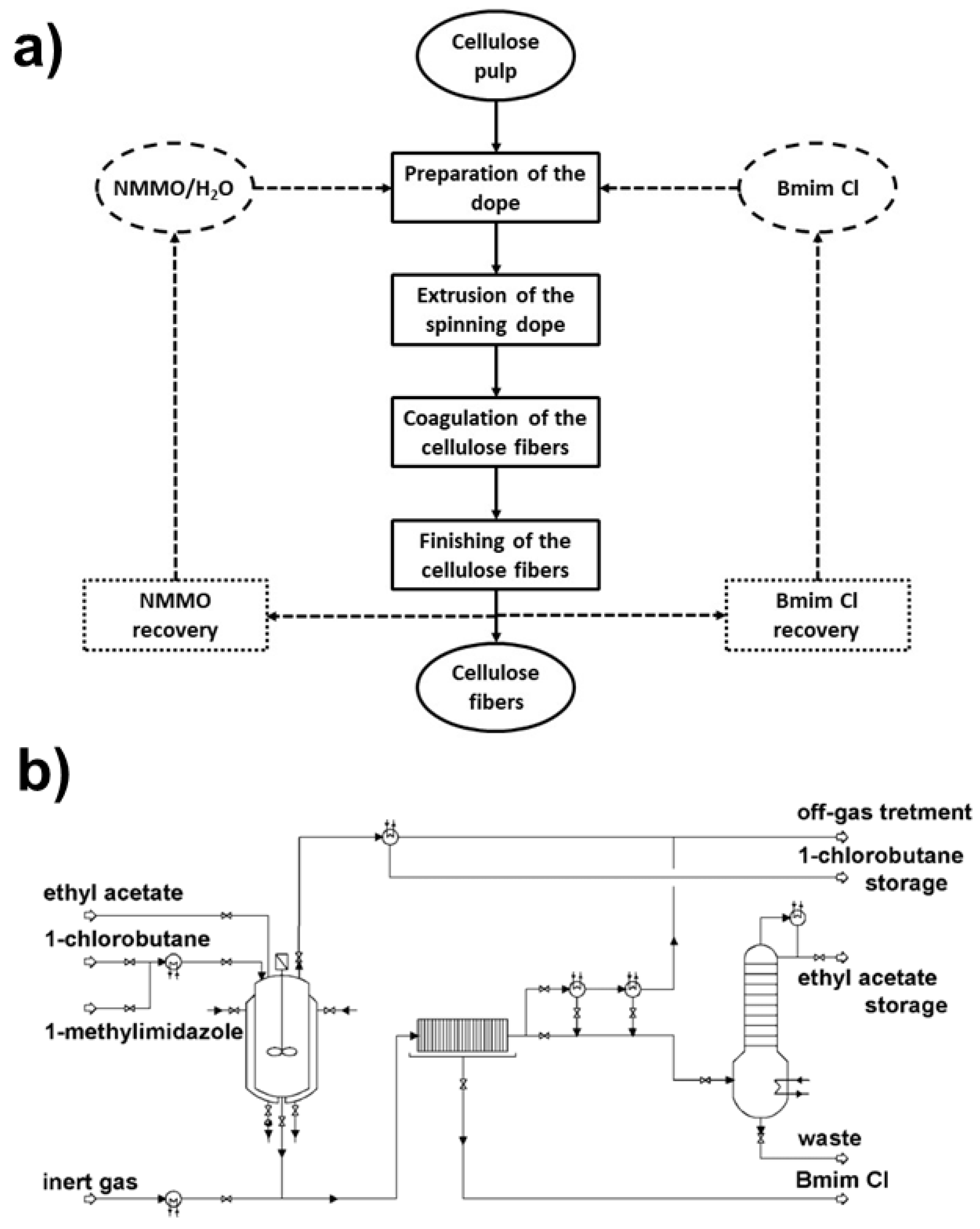
Monohydrated NMMO is a non-derivatizing solvent for cellulose in industry and it is used in the manufacturing of man-made fibers. The NMMO/H2O cellulose dissolution method developed by McCorsley [39] and used as comparison in a study on dissolution with ionic liquids by Kosan et al. [40] was adopted. Steps, process units and potentiality of the cellulose dissolution with BmimCl were taken to be equal to NMMO/H2O dissolution process modifying only the molar ratio between cellulose and solvent (1:6 instead of 1:8) and the spinning mass temperature (116 °C instead of 94 °C) as used by Kosan and coworkers on laboratory-scale [40]. These changes have been done to obtain similar mechanic characteristics of the fiber found by Kosan and co-authors in their approach. The block diagram for the alternative processes with BmimCl and with NMMO/H2O is shown in Figure 1a.
The work entailed the synthesis process modeling of NMMO, BmimCl and several of their precursors. The BmimCl synthesis method reported by Park and Kazlauskas [41] was adopted as the basis for the preliminary design of the industrial scale plant (reference potentiality of the production line: 5 × 10⁵ kg/year of Bmim Cl). Moreover, since 1-chlorobutane, ethyl acetate, 1-methylimidazolium and its precursors monomethylamine (CH3NH2) and glyoxal (CHOCHO) were not included in LCA databases, their industrial-scale chemical syntheses were developed by conceptual and preliminary detailed design activities (Table 1) according to relevant patents and technical literature [42,43,44,45,46,47].
For example, Figure 1b reports the Process Flow Diagram (PFD) developed for the industrial-scale synthesis of BmimCl. As can be observed in the picture, the synthesis occurs in a batch reactor, which is the direct scale-up of the batch process at lab-scale [41]. The preliminary sizing of the reactor (volume and dimensions) allowed the estimation of thermal (heating and cooling) and electric (stirring) inputs required by the unit. Similarly, the closure of the heat and material balances, also supported by the use of CPS software Aspen Plus® in the definition of material properties and equilibria, allowed the calculation of material and energy inputs and outputs for the whole plant (Table 3).
The same approach was followed for the NMMO synthesis: the data reported by Scholten and Rindtorff [48] and the N-methylmorpholine (NMM) synthesis method described by Simon et al. [49] were adopted as reference to design an industrial-scale process (reference potentiality of the production line: 2.5 × 10⁶ kg/year of NMMO). The related LCI of energy and material in input to the synthesis process of NMMO/H2O is reported in Table 4.
3.2. DMC-BioD Case Study
In this case study, Righi et al. [15] aimed at assessing the potential environmental impacts of the production process of dimethyl carbonate-biodiesel (DMC-BioD), an alternative biofuel to diesel which does not involve the production of glycerol [50]. The production process of DMC-BioD was compared to the production of conventional methanol (MeOH)-biodiesel and fossil diesel. This case represents a situation in which the innovative process, tested only at lab scale, has to be compared to already industry-ready and available in LCA databases processes [51]. The life cycle perspective adopted in the study required an in-depth analysis and modeling of the DMC-BioD synthesis process, for which limited information about the associated environmental impacts is available in the literature.
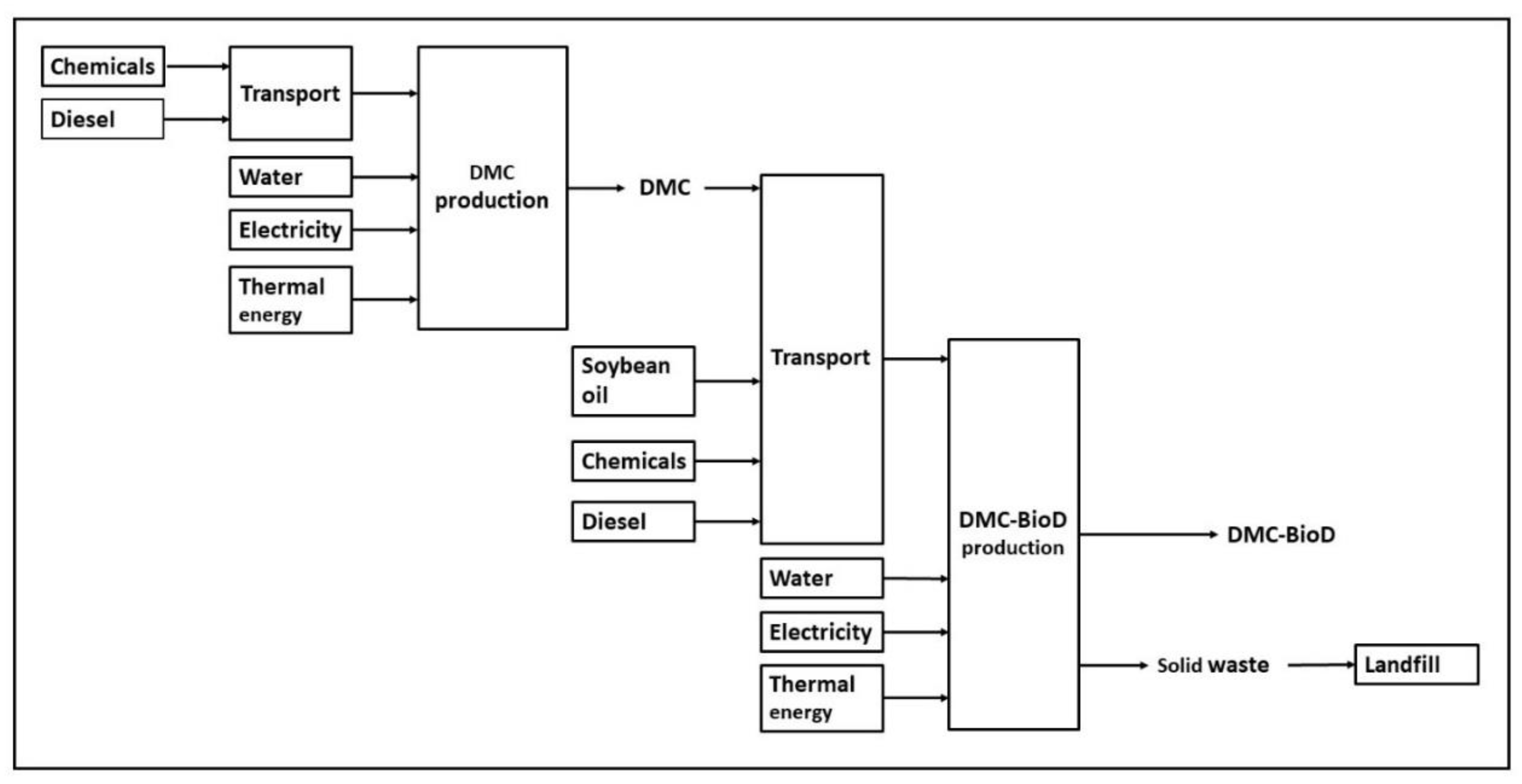
The system boundaries defined for the production processes assessed are “cradle-to-gate” and include all the unit processes from raw materials extraction to product manufacture, while product distribution and use in engines are excluded. Figure 2 shows the system boundaries of the production process of DMC-BioD. LCA databases [51,52] were used as source of background data for: (i) production of electricity and steam; (ii) transport systems; (iii) cultivation of soybean and soybean oil production; and (iv) production of chemicals involved in the process [15].
Modeling and Scale-Up of the Processes
DMC-BioD is obtained by the transesterification reaction of a triglyceride, or a mixture of triglycerides of fatty acids, with DMC in the presence of a base catalyst. The definition of a preliminary process flow diagram of the process from the available technical data [50,53] was based on the principia of good engineering practice in process design [11,12,13]. The estimated material and energy flows, as simulated with the support of Aspen HYSYS® [54], allowed the definition of the relevant inventory data (Table 5).
The work of Righi et al. [15] entailed also the synthesis process modeling of DMC through oxy-carbonylation process, not included in the available LCA databases. The oxy-carbonylation process was chosen among the various DMC production methods thanks to its potential environmental benefits: the avoided contamination from phosgene and the avoided disposal of byproduct inorganic salts. The oxy-carbonylation process developed by ENICHEM Company and detailed in Rivetti and Romano [55] was adopted as reference process.
3.3. PHA Extraction Case Study
Righi et al. [56] compared the environmental performance of the method proposed by Samorì et al. [57] for the extraction of poly-hydroxybutyrate (PHB) with dimethyl carbonate (DMC) from bacteria cells with the environmental performance of an alternative process using 1,2-dichloroethane (DCE), as detailed in the US Patent 4,324,907 [58]. This case represents a situation in which the innovative process, tested only at lab scale, has to be compared to an already industry-ready but not available in LCA databases process.
A “gate-to-gate” approach is used, and only the extraction process has been considered since the bacteria cultivation phase and the bioplastic product manufacture after the polymer extraction are assumed to be equivalent for all considered extraction processes. The system boundaries of the study include the following processes: biomass preparation, chemicals production, PHB extraction, chemicals recovery, air emissions abatement, and solid waste management [56].
This study compares four scenarios of the protocol proposed by Samorì et al. [57], which uses two different biomasses for extracting PHB with DMC: (a) dried biomass (Dry); and (b) microbial slurry (Slurry). For each biomass, two different recovery approaches have been evaluated: (1) the evaporation of the solvent (Evap); or (2) the addition of EtOH and precipitation (Precip).
Modeling and Scale-Up of the Processes
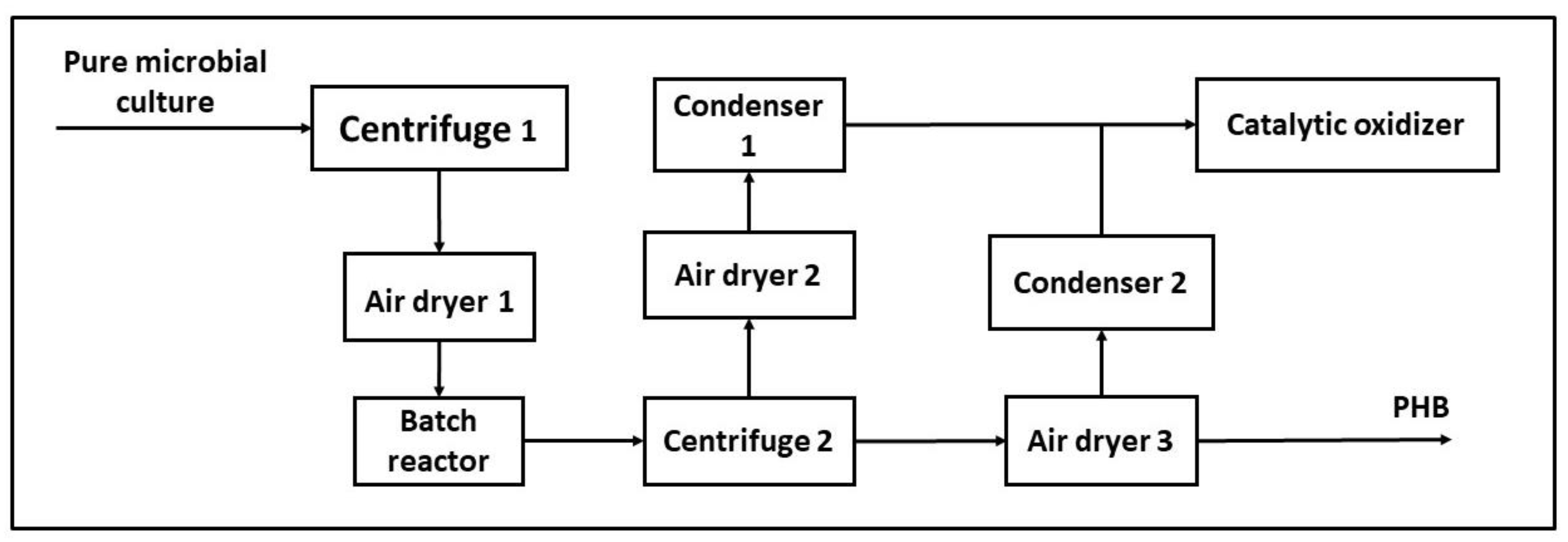
The protocol proposed by Samorì et al. [57] and the US Patent 4,324,907 [58] were adopted as reference documents. The five extraction processes at industrial scale have been proposed. The available data from these protocols are at lab scale and they only report information regarding mass balances and performance of the process such as: biomass/solvent ratio, recovery of PHB, temperature and duration of the extraction, and solvent/non-solvent ratio. For that reason, energy and material balances were solved, and the main equipment units were preliminarily sized based on relevant scientific and technical references and the CPS software (Aspen HYSYS® [54]) (Table 6). The extraction processes are composed by a series of equipment units: (1) centrifuges; (2) batch reaction vessels; (3) air dryers; (4) catalytic oxidizer; and (5) pervaporation systems (only in the scenarios where the polymer is recovered with the addition of EtOH). The equipment is different in size and arrangement depending on the different scenarios. For instance, those of the production scenario “Dry-Evap.” are shown in Figure 3. Table 7 shows a comparison between energy consumptions estimated by lab scale data and by industrial scale-up data of three extraction steps: centrifugation, drying and solubilization. Lab scale data have been estimated by multiplying the specific power of each equipment unit by the duration of its application. As shown in Table 7, data from laboratory scale are much higher than those obtained from industrial scale-up. Table 7 shows also that a further relevant aspect concerns chemicals recovery. It is not considered in the lab scale because avoiding waste and emission and saving reagents are not relevant objectives in this process life cycle stage. Instead, in the industrial scale-up, chemicals recovery is evaluated because reducing solvent consumption is a key aspect.
Table 8 shows the life cycle inventory obtained for “Dry-Evap.” scenario.
3.4. Use of Alternative Sorbents for Acid Gas Removal in Waste-to-Energy Plants
This case study represents a situation in which the process and materials to be analyzed are already industry ready, but the information is difficult to collect. The goal of the study is the evaluation of different dry treatment strategies for acid gas removal from flue gases of waste-to-energy (WtE) plant. The emission of airborne pollutants (e.g., hydrogen chloride, HCl) is the main drawback of the thermal treatment of solid waste [66,67]. The availability of new sorbent materials [68] poses to the designers of new treatment process critical choices that may affect the environmental impacts of the plant under design [69,70]. In a life cycle perspective, the choice of the best dry treatment solution should consider not only the acid gas removal efficiency, but also the indirect environmental burdens related to supply of sorbents and disposal of solid process residues.
Two issues arise in approaching these systems with a LCA method. The first issue is the lack of quantitative information about the removal performance of the different commercially available sorbents, which hinders the correct quantitation of the inventory flows needed to achieve a given HCl removal target. Sorbent suppliers and technology providers rarely disclose their data in the open literature [71], while scholarly studies mainly report results of laboratory-scale tests of little applicability to full-scale systems [72,73]. The second issue is related to the high variability of the composition of processed waste, which may result in significant fluctuation of HCl concentrations in the gases to be treated [74,75], hence the sensitivity of the LCI results to these parameters need to be thoughtfully checked. Being the relationship between removal efficiency and sorbent feed rate non-linear [76], process modeling is required for a correct evaluation of both aspects.
3.4.1. Modeling and Scale-Up of the Processes
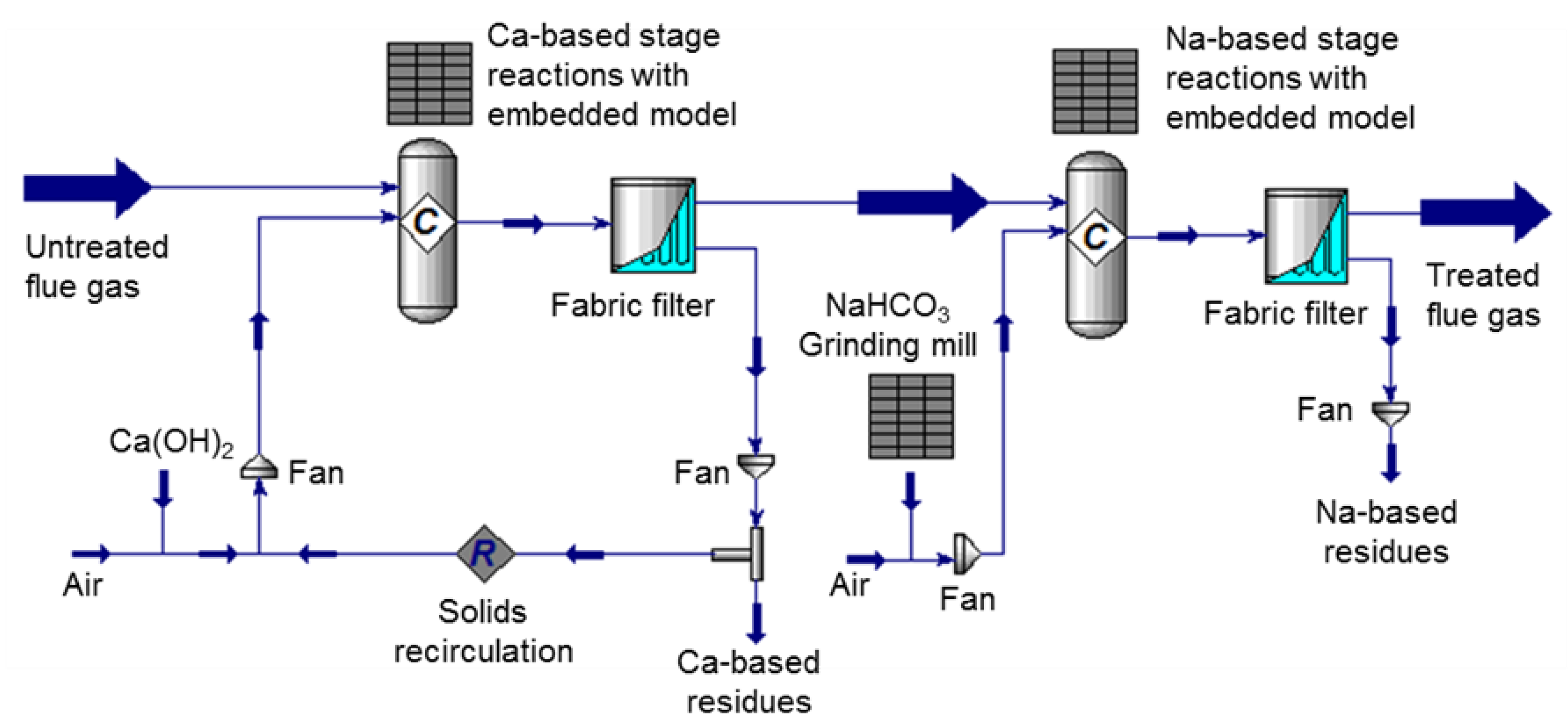
In this case study, the process is well established at industrial scale, so no conceptual definition of the Process Flow Diagram (PFD) is required. The reference dry acid gas treatment technology considered here is a two-stage system, based on the injection and subsequent filtering of calcium hydroxide, Ca(OH)2, and sodium bicarbonate, NaHCO3, respectively, in the 1st and 2nd treatment stage (Figure 4). These sorbents react with the acid pollutants via gas–solid reactions [77]. The spent solid residues are collected by the fabric filters. The two treatment stages have the following features:
- Ca-based stage. Calcium hydroxide is the less reactive of the two sorbents and it is only partially converted in the residence times typical of dry sorbent injection systems [78]. The solid residues of the reaction of Ca(OH)2 with acid gases, known as Ca-based residues (CBR), are to date non-recyclable and, thus, are to be sent to proper disposal sites [79]. Therefore, the Ca-based stage can be equipped with a solids recirculation system, which helps maximizing sorbent conversion.
- Na-based stage. Sodium bicarbonate presents higher affinity towards acid gases, but the sorbent as commercially supplied requires comminution in a grinding mill before injection to promote its reactivity [80]. In contrast with CBR, Na-based residues (NBR) can be recycled off-site: dedicated plants regenerate fresh bicarbonate from the residue, with ~85 wt % efficiency [81].
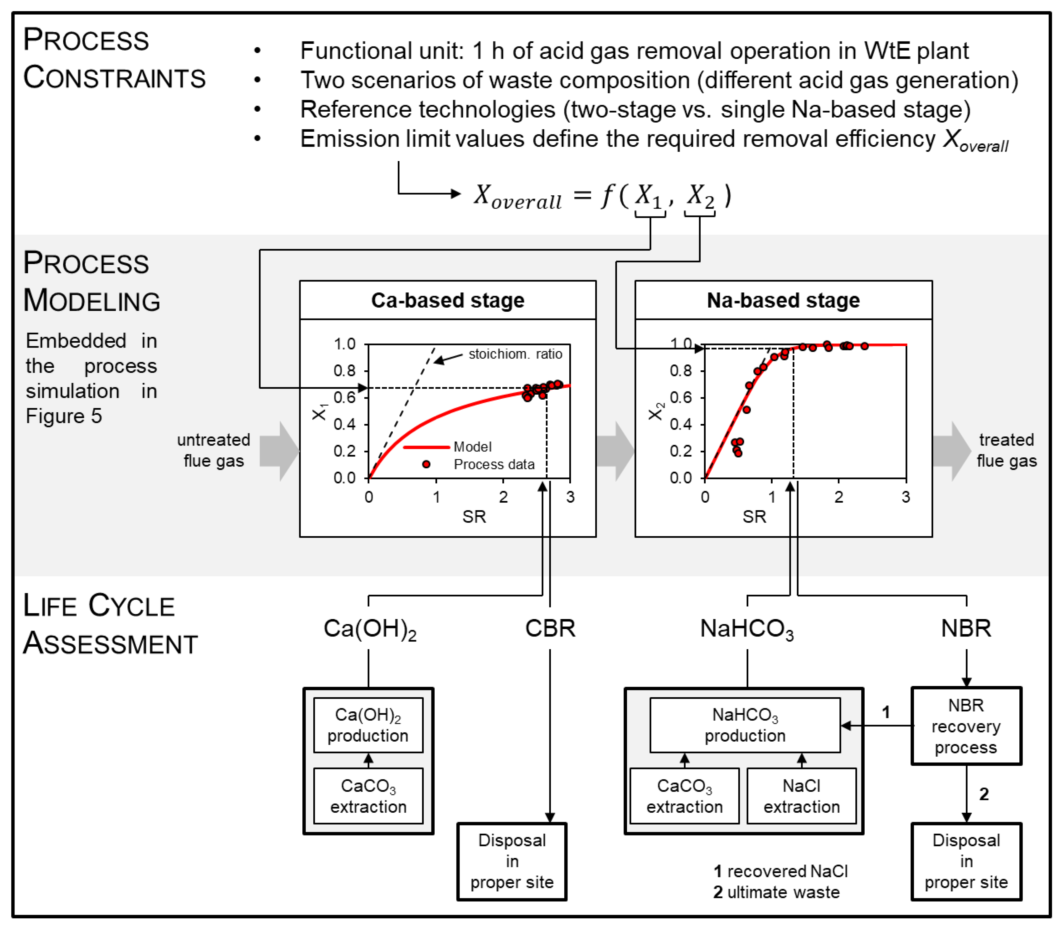
Figure 5 details the procedure adopted for the integration of the process simulation in a life cycle assessment framework. First, the functional unit (1 h of operation of a 360 t/day WtE plant), the waste types (a typical urban waste and a chlorine-rich waste representative of industrial refuses, see [69] for composition), and the emission limit value (2 mg/Nm3 for HCl) are set. As the LCA aims to evaluate the environmental consequences of varying the repartition of HCl removal efficiency X in the 1st calcium-based stage (X1) and in the 2nd sodium-based stage (X2), four reference process configurations are defined (Ca_0 in which only sodium bicarbonate is used; and Ca_25, Ca_50 and Ca_75 in which, respectively, 25 wt %, 50 wt % and 75 wt % of the incoming HCl is removed in the first Ca(OH)2-based stage).
Process modeling was based on the empirical reaction model described by Dal Pozzo et al. [74], calibrated on a set of process data from operating plants and expressing the non-linear relationship between the over-stoichiometric ratio (SR) of reactant fed to the system and the obtained acid gas conversion. The non-linear model linking SR and X for the Ca-based and the Na-based stages is shown in Figure 5, alongside the process data from the reference plant adopted for model calibration. The model was embedded in CPS software to quickly solve energy and material balances and derive contribution of the process to LCI. Figure 4 shows the flow diagram of the process in the simulation environment. The reaction model is the core of the simulation, quantifying the material streams (sorbents and residues) associated with the given HCl removal efficiency for the two stages. The operation of the ancillary equipment (dilute-phase pneumatic conveying for sorbent feed, milling for the sodium bicarbonate feed, dense-phase pneumatic conveying for the discharge and recirculation of residues, and air pulse cleaning for fabric filter) is simulated through specific software objects and/or simple external sub-models linked to the simulation, thus determining the energy requirements of the system (Table 9).
The mass flow rates of sorbents and residues obtained by process simulation define the mass and energy reference flows throughout the life cycle (Figure 5). Extraction and processing of raw materials, transportation phases and disposal are modeled using secondary data, viz. ELCD and CPM databases [82,83]. The process for regenerating the spent Na-based sorbent (NBR recycling process) is not available in the database and limited process data are disclosed in the open literature [81]. Thus, once more, the preliminary design procedure described for the previous case studies (definition of process flow diagram, energy and mass balances, unit operation modeling, preliminary unit sizing) was adopted starting from patent data [84] and availing of CPS software.
3.4.2. LCIA Results and Discussion
In this case study, three impact category indicators were used to illustrate the Life Cycle Impact Assessment (LCIA) results and the role of process simulation in determining them: acidification (AC, expressed in terms of kg SO2 eq.), carbon footprint (CF, expressed in terms of kg CO2 eq.), and primary energy consumption (PEC, expressed in terms of MJ). The characterization factors for the indicators were based on the CML-IA database [88].
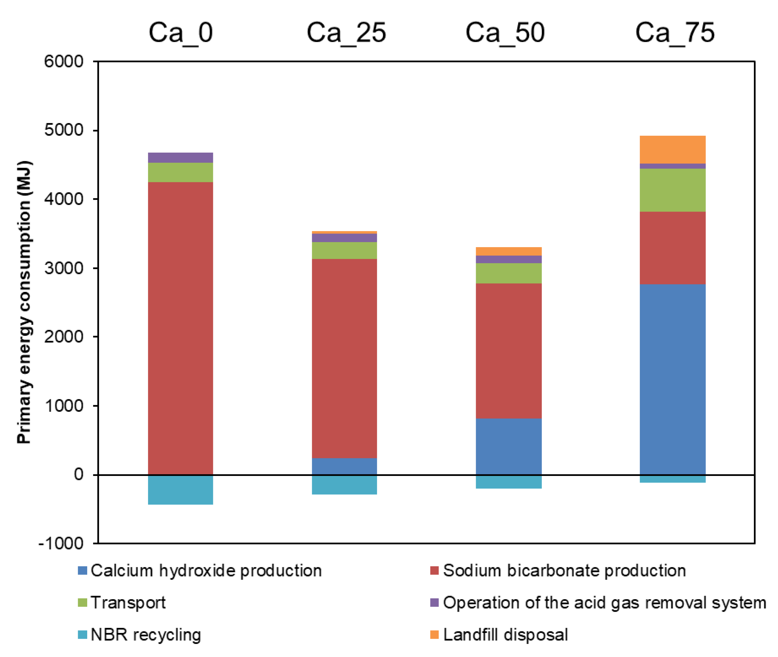
Figure 6 presents the energy consumption indicator (PEC), by detailing the contributions of the different unit processes to the overall indicator, with reference to the urban waste scenario. The production of sodium bicarbonate is, by far, the main contributor, due to the high demand of heat and electricity related to the extraction and processing of the raw materials (sodium chloride and limestone). By increasing the utilization of the Ca-based treatment stage, the share of the PEC indicator associated with the production of calcium hydroxide increases, but the share due to sodium bicarbonate decreases to a greater extent, causing the overall reduction of the PEC indicator. Only for the case Ca_75, the additional impact due to Ca(OH)2 production offsets the reduced demand of NaHCO3, resulting in an increase of the PEC indicator. The figure also highlights the minor role of the energy consumption arisen during the operation of the flue gas cleaning system, compared to the energy flows associated to the extraction and processing of raw materials. Only the 3.5% of the PEC impacts in the case Ca_0 and the 1.6% in the case Ca_75 are ascribed to the operation of the treatment system. As shown in Table 7, the most energy-intensive equipment is the air-classifying mill for the grinding of powdered sodium bicarbonate before the injection in the flue gas ductwork. Even if the utilization of two abatement stages (cases Ca_25 to Ca_75) imply the operation of an additional pneumatic transport line, the energy savings due to the reduction of the bicarbonate feed to be ground cause a lower overall energy consumption for the two-stage configurations than for the case Ca_0.
Lastly, it is shown that the NBR recovery process is associated with a negative contribution to the PEC indicator. The impact credits of the recycling process, i.e., the avoided energy consumption associated with the extraction of fresh brine, largely offset the impacts generated by the energy needs at the recycling plant. Indeed, the energy consumption at the plant, associated for the 95% to the power requirements of the filter press (see Table 7), is equal to just the 4.0% of the avoided energy consumption related to brine extraction.
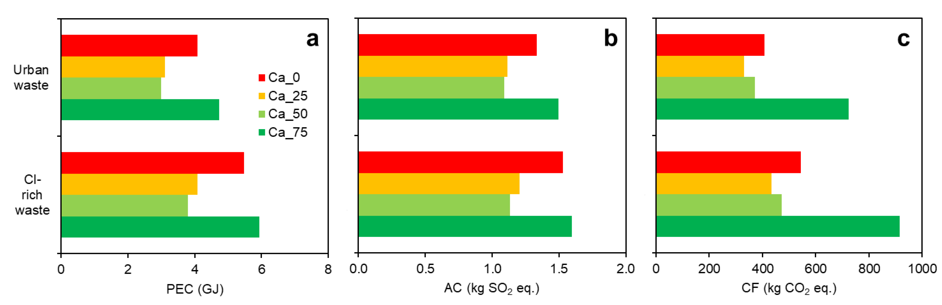
Figure 7 summarizes the three environmental indicators calculated for the four system configurations and the two waste composition scenarios. A higher utilization of the 1st Ca-based treatment stage results in lower impacts in the three environmental indicators considered as long as only a fraction of HCl is removed by the calcium hydroxide (cases Ca_25 and Ca_50). When compared to the single stage Na-based treatment, a two-stage system abating 50% of the HCl load in the first stage (Ca_50) generates an 18% reduction in the acidification indicator in the urban waste scenario, while the carbon footprint and the PEC shrink 8% and 27%, respectively. Conversely, demanding a 75% removal efficiency to the Ca-based stage (Ca_75) generates higher impacts (in particular, a 95% increase of the carbon footprint) due to the high stoichiometric excess of Ca(OH)2 required, as a consequence of the low reactivity of Ca(OH)2 mentioned in Section 3.4.1.
In the Cl-rich waste scenario, the Ca_50 configuration realizes a 26% reduction in the AC indicator, a 13% reduction in the CF indicator and a 31% reduction in the PEC indicator, with reference to the Ca_0 benchmark. It can be noticed that the environmental advantage of the Ca_50 configuration in the presence of Cl-rich waste is higher than in the case of urban waste. This is due to the higher removal efficiency required to meet the same emission target with a higher incoming HCl concentration, which entails a more-than-linear increase in the feed rate of NaHCO3 compared to the urban waste scenario. Therefore, the advantage of reducing the feed rate of NaHCO3 by removing a fixed fraction of the incoming HCl load in the Ca-based stage is greater. The key role of process modeling in correctly characterizing the process (in this case, by considering the non-linearity in the relationship between removal efficiency and sorbent feed) and thus identifying aspects that would be lost in a regular database-driven LCA approach where inventory entries and associated impacts are typically scaled linearly with the functional unit is evident.
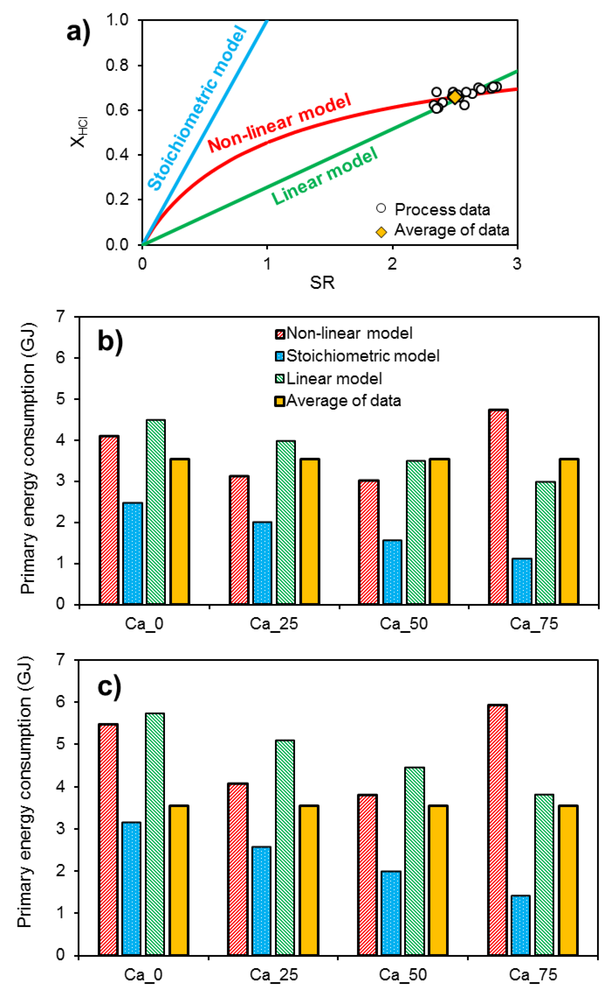
To demonstrate the importance on the LCIA results of the correct choice of a model in the preliminary design of the acid gas removal system, Figure 8 compares the PEC indicator obtained by different choices. Figure 8a illustrates four different ways to model HCl removal in the Ca-based stage. The previous discussion adopted the non-linear model (red curve) calibrated with a set of process data (Figure 5) to quantify the consumption of reactant associated with a given HCl removal efficiency. This option provides a description of the system closer to the real operative performance of sorbents. Conversely, the attempt to use plant data for evaluating LCA inventory, without developing a model for the conversion and the preliminary design of the process, would consider the average of process data (yellow diamond). This is the approach typically used in compiling LCI databases. In between these two cases, other alternative models are considered, featuring a simplified correlation between conversion and stoichiometric ratio (SR): the stoichiometric model (blue curve), which ignores mass transport and kinetic limitations in the reaction, and the linear model (green curve), which assumes proportionality among the considered parameters.
As evident in both the urban waste (Figure 8b) and the Cl-rich waste (Figure 8c) scenarios, the use of average process data (yellow diamond in Figure 8a) does not allow discriminating the different environmental impacts associated to the mode of operation of the acid gas treatment system. Moreover, the values obtained for the PEC indicator may differ as much as 60% from the results based on non-linear modeling.
The use of less precise models, such as linear and stoichiometric models, misestimate the reactivity of sorbents leading again to relevant discrepancies in the indicator results. Indeed, only the non-linear model is capable of considering both the different reactivity of the two sorbents and the “diminishing returns” in terms of removal efficiency of increasing sorbent feed rate, allowing to identify the optimal repartition of HCl removal between the two stages of the treatment system in terms of environmental impacts. This exemplifies that the quality of the approach followed in preliminary design may affect data and, in some cases, even frustrate the efforts invested in the activity.
4. Conclusions
The case studies described in this paper highlighted the use of process design techniques and modeling in tracking and quantifying the energy and material consumption entries associated to both the foreground and background processes of a life cycle. Even if a process is in its early development stage, good engineering practice and scaling rules, assisted by chemical process simulation software, allow drafting the information on the envisaged industrial-scale process at an adequate detail for the purpose of LCA, as shown in the case studies. The preliminary design approach considers all the energy streams required by the process, including utilities, and assesses their relevance. Furthermore, it avoids the overestimation of energy consumption that would be made by directly considering primary data from the laboratory scale, as evidenced in Case Study 3.
Another advantage of the integration of process modeling in the LCA framework is the flexibility provided by the simulation, which enables the study of the sensitivity of the environmental indicators as a function of the process conditions and design choices. For example, in Case Study 4, the effect of a different composition of the treated waste on the environmental burdens from the WtE plant was explored, evidencing the relative stability of the results at the change of HCl concentration in flue gases.
On the other hand, it has to be remarked that the adoption of process models to bridge gaps in available primary data requires due knowledge of the underlying chemical and physical characteristics of the process. With reference to Case Study 4, it was shown how the use of oversimplified models might produce significant discrepancies in the LCIA results.
Generally speaking, the case studies demonstrated that, while an actual scale-up would require extensive research efforts, the proposed simplified approach to process design is adequate to the scope of the exploratory LCA studies for new materials or emerging processes, for which datasets are not available in common LCI databases. Although no off-the-shelf solution is possible for the estimation of energy consumption and case-specific simulation and design activities are usually required, integrating the expertise of LCA practitioners and of process engineers is evidenced here as a key point in performing a reliable sustainability assessment of a new chemical product or process.
Author Contributions
Serena Righi and Alessandro Tugnoli conceived and designed the paper, and wrote the Introduction and Materials and Methods. Filippo Baioli and Alessandro Dal Pozzo wrote the Results and prepared figures and tables. Discussions and Conclusions were the collective work of all four authors.
Conflicts of Interest
The authors declare no conflict of interest.
Abbreviations
| Acronym | Term |
| AC | Acidification |
| BmimCl | 1-butyl-3-methylimidazolium chloride |
| CBR | Ca-based residues |
| CF | Carbon Footprint |
| CPS | Chemical Process Simulation |
| DCE | 1,2-dichloroethane |
| DMC | dimethyl carbonate |
| DMC-BioD | dimethyl carbonate-biodiesel |
| ELCD | European reference Life Cycle Database |
| EtOH | ethanol |
| FU | Functional Unit |
| I/O | Input/Output |
| ISO | International Organization for Standardization |
| LCA | Life Cycle Assessment |
| LCI | Life Cycle Inventory |
| LCIA | Life Cycle Impact Assessment |
| MeOH | methanol |
| NBR | Na-based residues |
| NMM | N-methylmorpholine |
| NMMO/H2O | N-methyl-morpholine-N-oxide monohydrated |
| PD | Preliminary design |
| PEC | Primary Energy Consumption |
| PFD | Process Flow Diagram |
| PHB | poly-hydroxybutyrate |
| PS | Preliminary sizing |
| R&D | Research and Development |
| SR | stoichiometric ratio |
| WtE | waste-to-energy plant |
References
- Ruiz-Mercado, G.J.; Smith, R.L.; Gonzalez, M.A. Sustainability indicators for chemical processes: I. Taxonomy. Ind. Eng. Chem. Res. 2012, 51, 2309–2328. [Google Scholar] [CrossRef]
- Tufvesson, L.M.; Tufvesson, P.; Woodley, J.M.; Borjesson, P. Life cycle assessment in green chemistry: Overview of key parameters and methodological concerns. Int. J. Life Cycle Assess. 2013, 18, 431–444. [Google Scholar] [CrossRef]
- Broeren, M.L.M.; Zijp, M.C.; Waaijers-van der Loop, S.L.; Heugens, E.H.W.; Posthuma, L.; Worrell, E.; Shen, L. Environmental assessment of bio-based chemicals in early-stage development: A review of methods and indicators. Biofuels Bioprod. Biorefin. 2017, 11, 701–718. [Google Scholar] [CrossRef]
- European Commission. Communication from the Commission to the Council and the European Parliament—Integrated Product Policy, Building on the Environmental Life-Cycle Thinking; COM (2003) 302 Final; European Commission: Brussels, Belgium, 2003. [Google Scholar]
- Environmental Management—Life Cycle Assessment—Principles and Framework; ISO 14040; ISO: Geneva, Switzerland, 2006.
- Hellweg, S.; Canals, L.M.I. Emerging approaches, challenges and opportunities in life cycle assessment. Science 2014, 344, 1109–1113. [Google Scholar] [CrossRef] [PubMed]
- UNEP/SETAC. Why Take a Life Cycle Approach? United Nations Publications: New York, NY, USA, 2004. [Google Scholar]
- Arvidsson, R.; Svanström, M. A Framework for Energy Use Indicators and Their Reporting in Life Cycle Assessment. Integr. Environ. Assess. Manag. 2016, 12, 429–436. [Google Scholar] [CrossRef] [PubMed]
- Huijbregts, M.A.J.; Hellweg, S.; Frischknecht, R.; Hendriks, H.W.M.; Hungerbühler, K.; Hendriks, A.J. Cumulative energy demand as predictor for the environmental burden of commodity production. Environ. Sci. Technol. 2010, 44, 2189–2196. [Google Scholar] [CrossRef] [PubMed] [Green Version]
- Huijbregts, M.A.J.; Rombouts, L.J.A.; Hellweg, S.; Frischknecht, R.; Hendriks, A.J.; van de Meent, D.; Ragas, A.M.J.; Reijnders, L.; Struijs, J. Is cumulative fossil energy demand a useful indicator for the environmental performance of products? Environ. Sci. Technol. 2006, 40, 641–648. [Google Scholar] [CrossRef] [PubMed]
- Sinnott, R.K. Coulson & Richardson’s Chemical Engineering, 3rd ed.; Butterworth-Heinemann: Oxford, UK, 1999; Volume 6. [Google Scholar]
- Bisio, A.; Kabel, R.L. Scale-Up of Chemical Processes: Conversion from Laboratory Scale Tests to Successful Commercial Size Design; Wiley: New York, NY, USA, 1985. [Google Scholar]
- Zlokarnik, M. Scale-Up in Chemical Engineering; Wiley: Weinheim, Germany, 2002. [Google Scholar]
- Righi, S.; Morfino, A.; Galletti, P.; Samorì, C.; Tugnoli, A.; Stramigioli, C. Comparative cradle-to-gate life cycle assessments of cellulose dissolution with 1-butyl-3-methylimidazolium chloride and N-methyl-morpholine-N-oxide. Green Chem. 2011, 13, 367–375. [Google Scholar] [CrossRef]
- Righi, S.; Bandini, V.; Fabbri, D.; Cordella, M.; Stramigioli, C.; Tugnoli, A. Modeling of an alternative process technology for biofuel production and assessment of its environmental impacts. J. Clean. Prod. 2016, 122, 42–51. [Google Scholar] [CrossRef]
- Guthrie, K.M. Data and techniques for preliminary capital cost estimating. Chem. Eng. 1969, 76, 114–142. [Google Scholar]
- Remer, D.S.; Chai, L.H. Estimate costs of scaled-up process plants. Chem. Eng. 1990, 97, 138–175. [Google Scholar]
- Caduff, M.; Huijbregts, M.A.J.; Koehler, A.; Althaus, H.-J.; Hellweg, S. Scaling Relationships in Life Cycle Assessment. J. Ind. Ecol. 2014, 18, 393–406. [Google Scholar] [CrossRef]
- Wernet, G.; Papadokonstantakis, S.; Hellweg, S.; Hungerbuhler, K. Bridging data gaps in environmental assessments: Modeling impacts of fine and basic chemical production. Green Chem. 2009, 11, 1826–1831. [Google Scholar] [CrossRef]
- Calvo-Serrano, R.; Gonzalez-Miquel, M.; Papadokonstantakis, S.; Guillen-Gosalbez, G. Predicting the cradle-to-gate environmental impact of chemicals from molecular descriptors and thermodynamic properties via mixed-integer programming. Comput. Chem. Eng. 2018, 108, 179–193. [Google Scholar] [CrossRef]
- Piccinno, F.; Hischier, R.; Seeger, S.; Som, C. From laboratory to industrial scale: A scale-up framework for chemical processes in life cycle assessment studies. J. Clean. Prod. 2016, 135, 1085–1097. [Google Scholar] [CrossRef]
- Caduff, M.; Huijbregts, M.A.J.; Althaus, H.-J.; Hendriks, A.J. Power-Law Relationships for Estimating Mass, Fuel Consumption and Costs of Energy Conversion Equipments. Environ. Sci. Technol. 2011, 45, 751–754. [Google Scholar] [CrossRef] [PubMed]
- Shibasaki, M.; Fischer, M.; Barthel, L. Effects on life cycle assessment d Scale up of processes. In Advances in Life Cycle Engineering for Sustainable Manufacturing Businesses; Takata, S., Umeda, Y., Eds.; Springer: London, UK, 2007; pp. 377–381. [Google Scholar]
- Zhou, Y.; Lee, C.K.; Sharratt, P. Bridging the Gap from Pilot Plant Experimental Records to Life Cycle Inventory. Ind. Eng. Chem. Res. 2017, 56, 10393–10412. [Google Scholar] [CrossRef]
- Smith, R.L.; Ruiz-Mercado, G.J.; Meyer, D.E.; Gonzalez, M.A.; Abraham, J.P.; Barrett, W.M.; Randall, P.M. Coupling Computer-Aided Process Simulation and Estimations of Emissions and Land Use for Rapid Life Cycle Inventory Modeling. ACS Sustain. Chem. Eng. 2017, 5, 3786–3794. [Google Scholar] [CrossRef]
- Zaimes, G.G.; Beck, A.W.; Janupala, R.R.; Resasco, D.E.; Crossley, S.P.; Lobban, L.L.; Khanna, V. Multistage torrefaction and in situ catalytic upgrading to hydrocarbon biofuels: Analysis of life cycle energy use and greenhouse gas emissions. Energy Environ. Sci. 2017, 10, 1034–1050. [Google Scholar] [CrossRef]
- Winjobi, O.; Shonnard, D.R.; Zhou, W. Production of Hydrocarbon Fuel Using Two-Step Torrefaction and Fast Pyrolysis of Pine. Part 1: Techno-economic Analysis. ACS Sustain. Chem. Eng. 2017, 5, 4529–4540. [Google Scholar] [CrossRef]
- Lari, G.M.; Pastore, G.; Haus, M.; Ding, Y.; Papadokonstantakis, S.; Mondelli, C.; Perez-Ramirez, J. Environmental and economical perspectives of a glycerol biorefinery. Energy Environ. Sci. 2018. [Google Scholar] [CrossRef]
- Schakel, W.; Hung, C.R.; Tokheim, L.-A.; Stromman, A.-H.; Worrell, E.; Ramirez, A. Impact of fuel selection on the environmental performance of post-combustion calcium looping applied to a cement plant. Appl. Energy 2018, 210, 75–87. [Google Scholar] [CrossRef]
- Environmental Management—Life Cycle Assessment—Requirements and Guidelines; ISO 14044; ISO: Geneva, Switzerland, 2006.
- Sugiyama, H.; Hirao, M.; Fischer, U.; Hungerbühler, K. Activity modeling for integrating environmental, health and safety (EHS) consideration as a new element in industrial chemical process design. J. Chem. Eng. Jpn. 2008, 41, 884–897. [Google Scholar] [CrossRef]
- Sugiyama, H.; Fischer, U.; Hungerbühler, K.; Hirao, M. Decision framework for chemical process design including different stages of environmental, health, and safety assessment. AIChE J. 2008, 54, 1037–1053. [Google Scholar] [CrossRef]
- Piccinno, F.; Hischier, R.; Seeger, S.; Som, C. Predicting the environmental impact of a future nanocellulose production at industrial scale: Application of the life cycle assessment scale-up framework. J. Clean. Prod. 2018, 174, 283–295. [Google Scholar] [CrossRef]
- Ayres, R.U. Life cycle analysis: A critique. Resour. Conserv. Recycl. 1995, 14, 199–223. [Google Scholar] [CrossRef]
- Tugnoli, A.; Santarelli, F.; Cozzani, V. An approach to quantitative sustainability assessment in the early stages of process design. Environ. Sci. Technol. 2008, 42, 4555–4562. [Google Scholar] [CrossRef] [PubMed]
- Alexander, B.; Barton, G.; Petrie, J.; Romagnoli, J. Process synthesis and optimization tools for environmental design: Methodology and structure. Comput. Chem. Eng. 2000, 24, 1195–1200. [Google Scholar] [CrossRef]
- Brunet, R.; Cortés, D.; Guillén-Gosalbez, G.; Jiménez, L.; Boer, D. Minimization of the LCA impact of thermodynamic cycles using a combined simulation-optimization approach. Appl. Therm. Eng. 2012, 48, 367–377. [Google Scholar] [CrossRef]
- Aspen Plus® 10.2-1. Aspen Technology Inc.: Burlington, MA, USA, 2000.
- McCorsley, C.C.; Asheville, N.C. Process for Shaped Cellulose Article Prepared from a Solution Containing Cellulose Dissolved in a Tertiary Amine N-Oxide Solvent. U.S. Patent 4,246,221, 20 January 1981. [Google Scholar]
- Kosan, B.; Michels, C.; Meister, F. Dissolution and forming of cellulose with ionic liquids. Cellulose 2008, 15, 59–66. [Google Scholar] [CrossRef]
- Park, S.; Kazlauskas, R.J. Improved Preparation and Use of Room-Temperature Ionic Liquids in Lipase-Catalyzed Enantio- and Regioselective Acylations. J. Org. Chem. 2001, 66, 8395–8401. [Google Scholar] [CrossRef] [PubMed]
- Hydrocarbon Processing; The Leonard Process Company: North Hollywood, CA, USA, 1979; Volume 58, p. 194f.
- Forkner, M.W.; Robson, J.H.; Snellings, W.M. Kirk-Othmer Encyclopedia of Chemical Technology, 4th ed.; Wiley: New York, NY, USA, 1994; Volume 12, p. 695. [Google Scholar]
- Mattioda, G.; Blanc, A. Ullmann’s Encyclopedia of Industrial Chemistry, 5th ed.; Verlag Chemie: New York, NY, USA, 1989; Volume A12, p. 491. [Google Scholar]
- Howe, B.K.; Hardy, F.R.F.; Clarke, D.A. Vapour Phase Oxidation of Hydroxy Compounds. GB Patent 1,272,592, 3 May 1972. [Google Scholar]
- Ebel, K.; Koehle, H.; Gamer, A.; Jäckh, A. Ullmann’s Encyclopedia of Industrial Chemistry, 5th ed.; Verlag Chemie: New York, NY, USA, 1989; Volume A13, p. 661. [Google Scholar]
- Von Däniken, A.; Chudacoff, M. Vergleichende ökologische Bewertung von Anstrichstoffen in Baubereich. Band 2: Daten; Buwal Schriftenreihe Unwelt Nr. 232: Bern, Switzerland, 1995. [Google Scholar]
- Scholten, H.; Rindtorff, K. Process for Producing Aqueous N-Methylmorpholine-N-oxide Solutions. U.S. Patent 4,748,241, 31 May 1988. [Google Scholar]
- Simon, J.; Becker, R.; Lebkücher, R.; Neuhauser, H. N-Alkylation of Amines. U.S. Patent 5,917,039, 29 June 1999. [Google Scholar]
- Fabbri, D.; Bevoni, V.; Notari, M.; Rivetti, F. Properties of a Potential Biofuel Obtained from Soybean Oil by Transmethylation with Dimethyl Carbonate. Fuel 2007, 86, 690–697. [Google Scholar] [CrossRef]
- Ecoinvent Centre. Ecoinvent Data and Reports v2.0 Final Reports Ecoinvent 2000; Swiss Centre for Life Cycle Inventories: Dübendorf, Switerland, 2007. [Google Scholar]
- GaBi Professional Database. Available online: http://www.gabisoftware.com/support/gabi/ (accessed on 20 August 2015).
- Notari, M.; Rivetti, F. Use of a Mixture of Esters of Fatty Acids as Fuel or Solvent. Patent WO 2004/052874, 24 June 2004. [Google Scholar]
- Aspen HYSYS 7.1. User’s Guide; Aspen Technology Inc.: Burlington, MA, USA, 2009.
- Rivetti, F.; Romano, U. Procedure for the Production of Alkyl Carbonates. Patent EP534545, 19 September 1992. [Google Scholar]
- Righi, S.; Baioli, F.; Samorì, C.; Galletti, P.; Tagliavini, E.; Stramigioli, C.; Tugnoli, A.; Fantke, P. A life cycle assessment of poly-hydroxybutyrate extraction from microbial biomass using dimethyl carbonate. J. Clean. Prod. 2017, 168, 692–707. [Google Scholar] [CrossRef]
- Samorì, C.; Basaglia, M.; Casella, S.; Favaro, L.; Galletti, P.; Giorgini, L.; Marchi, D.; Mazzocchetti, L.; Torri, C.; Tagliavini, E. Dimethyl carbonate and switchable anionic surfactants: Two effective tools for the extraction of polyhydroxyalkanoates from microbial biomass. Green Chem. 2015, 17, 1047–1056. [Google Scholar] [CrossRef]
- Senior, P.J.; Wright, L.F.; Alderson, B. Extraction Process. U.S. Patent 4,324,907, 13 April 1982. [Google Scholar]
- Perry, R.H.; Green, D.W.; Maloney, J.O. Perry’s Chemical Engineers’ Handbook, 6th ed.; McGraw-Hill: New-York, NY, USA, 1984. [Google Scholar]
- Harding, K.G.; Dennis, J.S.; von Blottnitz, H.; Harrison, S.T.L. Environmental analysis of plastic production processes: Comparing petroleum-based polypropylene and polyethylene with biologically-based poly-b-hydroxybutyric acid using life cycle analysis. J. Biotechnol. 2007, 130, 57–66. [Google Scholar] [CrossRef] [PubMed]
- Morfino, A. Collection, Production and Analysis of the Inventory Data of the Life Cycle of the Ionic Liquid Bmim-BF4 (In Italian). Bachelor’s Thesis, University of Bologna, Bologna, Italy, 2009; p. 91. [Google Scholar]
- Baker, C.G.J.; McKenzie, K.A. Energy consumption of industrial spray dryers. Dry. Technol. 2005, 23, 365–386. [Google Scholar] [CrossRef]
- EEA. EMEP/EEA Air Pollutant Emission Inventory Guidebook 2013; Technical Guidance to Prepare National Emission Inventories; EEA Technical Report 12; Publications Office of the European Union: Luxembourg, 2013. [Google Scholar]
- Kujawski, W. Application of pervaporation and vapor permeation in environmental protection. Pol. J. Environ. Stud. 2000, 9, 13–26. [Google Scholar]
- Neel, J. Introduction to Pervaporation. Pervaporation Membrane Separation Processes; Elsevier: Amsterdam, The Netherlands, 1991. [Google Scholar]
- Chi, C.; Li, Y.; Sun, R.; Ma, X.; Duan, L.; Wang, Z. HCl removal performance of Mg-stabilized carbide slag from carbonation/calcination cycles for CO2 capture. RSC Adv. 2016, 6, 104303–104310. [Google Scholar] [CrossRef]
- Damgaard, A.; Riber, C.; Fruergaard, T.; Hulgaard, T.; Christensen, T.H. Life cycle assessment of the historical development of air pollution control and energy recovery in waste incineration. Waste Manag. 2010, 30, 1244–1250. [Google Scholar] [CrossRef] [PubMed] [Green Version]
- Hunt, G.; Heiszwolf, J.J.; Sewell, M. Enhanced Hydrated Lime—A Simple Solution for Acid Gas Compliance. IEEE Trans. Ind. Appl. 2017, 54, 796–807. [Google Scholar] [CrossRef]
- Dal Pozzo, A.; Guglielmi, D.; Antonioni, G.; Tugnoli, A. Sustainability analysis of dry treatment technologies for acid gas removal in waste-to-energy plants. J. Clean. Prod. 2017, 162, 1061–1074. [Google Scholar] [CrossRef]
- Dal Pozzo, A.; Guglielmi, D.; Antonioni, G.; Tugnoli, A. Two-stage vs. single stage acid gas treatment systems: A performance assessment based on economic and environmental indices. In Proceedings of the 9th International Conference on Environmental Engineering and Management (ICEEM09), Bologna, Italy, 6–9 September 2017. [Google Scholar]
- Foo, R.; Berger, R.; Heiszwolf, J.J. Reaction Kinetic Modeling of DSI for MATS Compliance. In Proceedings of the Power Plant Pollutant Control and Carbon Management “MEGA” Symposium, Baltimore, MD, USA, 16–19 August 2016. [Google Scholar]
- Marocco, L.; Mora, A. CFD modeling of the Dry-Sorbent-Injection process for flue gas desulfurization using hydrated lime. Sep. Purif. Technol. 2013, 108, 205–214. [Google Scholar] [CrossRef]
- Gutiérrez Ortiz, F.J.; Ollero, P. A realistic approach to modeling an in-duct desulfurization process based on an experimental pilot plant study. Chem. Eng. J. 2008, 141, 141–150. [Google Scholar] [CrossRef]
- Dal Pozzo, A.; Antonioni, G.; Guglielmi, D.; Stramigioli, C.; Cozzani, V. Comparison of alternative flue gas dry treatment technologies in waste-to-energy processes. Waste Manag. 2016, 51, 81–90. [Google Scholar] [CrossRef] [PubMed]
- Kim, K.-D.; Jeon, S.-M.; Hasolli, N.; Lee, K.-S.; Lee, J.-R.; Han, J.-W.; Kim, H.-T.; Park, Y.-O. HCl removal characteristics of calcium hydroxide at the dry-type sorbent reaction accelerator using municipal waste incinerator flue gas at a real site. Korean J. Chem. Eng. 2017, 34, 747–756. [Google Scholar] [CrossRef]
- Brna, T.G. Cleaning of Flue Gases from Waste Combustors. Combust. Sci. Technol. 1990, 74, 83–98. [Google Scholar] [CrossRef]
- Antonioni, G.; Dal Pozzo, A.; Guglielmi, D.; Tugnoli, A.; Cozzani, V. Enhanced modelling of heterogeneous gas-solid reactions in acid gas removal dry processes. Chem. Eng. Sci. 2016, 148, 140–154. [Google Scholar] [CrossRef]
- Dal Pozzo, A.; Moricone, R.; Antonioni, G.; Tugnoli, A.; Cozzani, V. Hydrogen Chloride Removal from Flue Gas by Low-Temperature Reaction with Calcium Hydroxide. Energy Fuels 2018, 32, 747–756. [Google Scholar] [CrossRef]
- Margallo, M.; Taddei, M.B.M.; Hernandez-Pellon, A.; Aldaco, R.; Irabien, A. Environmental sustainability assessment of the management of municipal solid waste incineration residues: A review of the current situation. Clean. Technol. Environ. Policy 2015, 17, 1333–1353. [Google Scholar] [CrossRef]
- Walawska, B.; Szymanek, A.; Pajdak, A.; Nowak, M. Flue gas desulfurization by mechanically and thermally activated sodium bicarbonate. Pol. J. Chem. Technol. 2014, 16, 56–62. [Google Scholar] [CrossRef]
- Brivio, S. The SOLVAL platform: A sodium sludges valorization, an industrial reality for the environment (in Italian). L’Ambiente 2005, 3, 48–49. [Google Scholar]
- ELCD. European Reference Life Cycle Database. Available online: eplca.jrc.ec.europa.eu/ELCD3/index.xhtml (accessed on 2 February 2018).
- Swedish Life Cycle Center. CPM LCA Database. Available online: cpmdatabase.cpm.chalmers.se (accessed on 2 February 2018).
- Ninane, L.; Adam, J.F.; Humblot, C. Method for Producing an Aqueous Industrial Sodium Chloride Solution. U.S. Patent 5478447, 26 December 1995. [Google Scholar]
- Molerus, O. Overview: Pneumatic transport of solids. Powder Technol. 1996, 88, 309–321. [Google Scholar] [CrossRef]
- US EPA. Air Pollution Control Cost Manual, 6th ed.; United States Environmental Protection Agency Office of Air Quality Planning and Standards: Research Triangle Park, NC, USA, 2002. Available online: www3.epa.gov/ttncatc1/dir1/c_allchs.pdf (accessed on 2 February 2018).
- European Commission. Reference Document on BAT in Common Waste Water and Waste Gas Treatment/Management Systems in the Chemical Sector; Technical Report; Publications Office of the European Union: Luxembourg, 2016; Available online: https://ec.europa.eu/jrc/en/publication/eur-scientific-and-technical-research-reports/best-available-techniques-bat-reference-document-common-waste-water-and-waste-gas (accessed on 2 February 2018).
- Institute of Environmental Sciences (CML). CML-IA Characterization Factors; Universiteit Leiden: Leiden, The Netherlands, 2016; Available online: www.universiteitleiden.nl/en/research/research-output/science/cml-ia-characterisation-factors (accessed on 2 February 2018).
Figure 1.
(a) Alternative block diagram of cellulose dissolution (left branch with BmimCl and right branch with NMMO/H2O); and (b) process Flow Diagram considered for BmimCl production [14].
Figure 1.
(a) Alternative block diagram of cellulose dissolution (left branch with BmimCl and right branch with NMMO/H2O); and (b) process Flow Diagram considered for BmimCl production [14].

Figure 2.
System boundaries of the production process of dimethyl carbonate-biodiesel (DMC-BioD). “DMC production” and “DMC-BioD production” were modeled via Aspen HYSYS® [15].
Figure 2.
System boundaries of the production process of dimethyl carbonate-biodiesel (DMC-BioD). “DMC production” and “DMC-BioD production” were modeled via Aspen HYSYS® [15].

Figure 3.
Process block diagram of production scenario “Dry-Evap.” [56].
Figure 3.
Process block diagram of production scenario “Dry-Evap.” [56].

Figure 4.
Process flow diagram of the two-stage acid gas treatment system in the adopted chemical process simulation software.
Figure 4.
Process flow diagram of the two-stage acid gas treatment system in the adopted chemical process simulation software.

Figure 5.
Sketch of the integration between process modeling and life cycle assessment in the case study of alternative sorbents for acid gas removal.
Figure 5.
Sketch of the integration between process modeling and life cycle assessment in the case study of alternative sorbents for acid gas removal.

Figure 6.
Contribution of the different LCA unit processes to the primary energy consumption indicator. Waste composition scenario: urban waste.
Figure 6.
Contribution of the different LCA unit processes to the primary energy consumption indicator. Waste composition scenario: urban waste.

Figure 7.
Scores of the different acid gas treatment configurations analyzed in the case of urban waste and Cl-rich waste in the three impact category indicators: (a) primary energy consumption (PEC); (b) acidification (AC); and (c) carbon footprint (CF).
Figure 7.
Scores of the different acid gas treatment configurations analyzed in the case of urban waste and Cl-rich waste in the three impact category indicators: (a) primary energy consumption (PEC); (b) acidification (AC); and (c) carbon footprint (CF).

Figure 8.
Comparison of the influence on Life Cycle Impact Assessment (LCIA) results of different approaches to HCl removal modeling: (a) correlation between conversion of HCl and SR in the alternative models for Ca(OH)2 stage; (b) PEC indicator results (urban waste scenario); and (c) PEC indicator results (Cl-rich waste scenario).


Table 1.
Process design life cycle and data available for Life Cycle Inventory (LCI).
| Process Life Cycle Stage | Process Chemistry | Conceptual Design | Detailed Design | Plant Operation |
|---|---|---|---|---|
| Design activities | Selection of the chemical route and operative conditions | Process definition | Equipment and layout design, utilities design | Plant management and optimization |
| Information available | Stoichiometry, yields, temperature, pressure | Unit operations, energy and material balances | Equipment type and size, piping and instrumentation, operating procedure | Field data on energy and material balances |
| LCI modeling: Material input/output | Main raw materials and products | Raw materials, products and wastes | Raw materials, products, wastes, fugitive emissions | Raw materials, products, wastes, fugitive emissions |
| LCI modeling: Energy input/output | None | Process related energy demand | Plant energy demand (including losses) | Plant energy demand (including losses) |
| Data quality for LCI | Measured (in laboratory conditions) | Estimated data (process specific) | Estimated data (plant specific) | Measured data (plant specific) |
Table 2.
Synopsis of the case studies analyzed in the paper.
| Case Study | Problem with Data Availability | Modeling Based Directly on Available Data | Modeling Assisted by Preliminary Process Design | |||||
|---|---|---|---|---|---|---|---|---|
| Practical Problem | Unit Processes Affected | Available Data | I/O Contribution to LCI | Modeling Approach | I/O Contribution to LCI | |||
| Material I/O | Energy I/O | Material I/O | Energy I/O | |||||
| Case study 1 NMMO/H2O process | Industrial level application but no access to plant data | Cellulose dissolution by NMMO/H2O | Literature data on dissolution process Limited data on solvent recovery | Main input/output No data on solvent losses | No data available | PD of the process PS of the main equipment | Estimated input/output | Estimated thermal (including losses) and electric energy |
| NMMO synthesis | Limited literature data on chemical synthesis process, no data on product separation | Main input/output | No data available | PD of the process PS of the main equipment | Estimated input/output | Estimated thermal (including losses) and electric energy | ||
| Case study 1 Ionic liquid | Lab scale application only | Cellulose dissolution by BmimCl | No process data (laboratory scale solubility test) | No data available | No data available | PD of the process and PS of the equipment based on the NMMO/ H2O case | Estimated input/output | Estimated thermal (including losses) and electric energy |
| BmimCl systhesis | Laboratory synthesis protocol | Input/output at laboratory scale (not optimized) | Data for laboratory scale equipment | PD of the process PS of the main equipment | Estimated input/output | Estimated thermal (including losses) and electric energy | ||
| Case study 2 DMC-BioD | Lab scale application only + Industrial level application but no access to plant data | DMC-BioD production | Laboratory synthesis protocol | Input/output at laboratory scale (not optimized) | Data for laboratory scale equipment | PD of the process PS of the main equipment | Estimated input/output | Estimated thermal (including losses) and electric energy |
| DMC production | Limited literature data on production process | Main input/output | No data available | PD of the process PS of the main equipment | Estimated input/output | Estimated thermal (including losses) and electric energy | ||
| Case study 3 PHA extraction by DMC | Lab scale application only | Extraction process | Laboratory synthesis protocol | Input/output at laboratory scale (not optimized) | Data for laboratory scale equipment | PD of the process PS of the main equipment | Estimated input/output | Estimated thermal (incl. losses) and electric energy |
| Case study 3 PHA extraction by 1,2-DCE | Industrial level application but no access to plant data | Extraction process | Limited literature data on process | Main input/output | No data available | PD of the process PS of the main equipment | Estimated input/output | Estimated thermal (including losses) and electric energy |
| Case study 4 Sorbents for acid gas removal | Industrial level application but limited access to plant data | Flue gas treatment system at the WtE plant | Available plant data refer to specific modes of operation of the process (not optimized) | Main input/output data (no optimization or correlation to waste type) | Data available for specific operative condition | Non-linear model of the reaction, PD of the process, PS of the main equipment | Estimated input/output for different modes of operation | Estimated energy consumption for different modes of operation |
PD: preliminary design; PS: Preliminary sizing; I/O: input/output.
Table 3.
Synthesis processes modeled through Aspen Plus ® involved in the BmimCl. All values are referred to 1 kg of BmimCl produced in an industrial plant of 500 t/year [14].
Table 3.
Synthesis processes modeled through Aspen Plus ® involved in the BmimCl. All values are referred to 1 kg of BmimCl produced in an industrial plant of 500 t/year [14].
| Process | IO | Flow | Unit | Value |
|---|---|---|---|---|
| Glyoxal production | Input | Thermal energy | MJ | 1.53 |
| Electric energy | MJ | 0.43 | ||
| Ethylene glycol | kg | 2.03 | ||
| Output | Glyoxal | kg | 1.16 | |
| Methylamine production | Input | Thermal energy | MJ | 1.86 |
| Electric energy | MJ | 0.02 | ||
| Ammonia | kg | 0.14 | ||
| Methanol | kg | 0.27 | ||
| Output | Methylamine | kg | 0.25 | |
| 1-methylimidazole production | Input | Thermal energy | MJ | 0.74 |
| Electric energy | MJ | 0.48 | ||
| Ammonia | kg | 0.14 | ||
| Formaldehyde | kg | 0.65 | ||
| Glyoxal | kg | 1.16 | ||
| Methylamine | kg | 0.25 | ||
| Output | 1-methylimidazole | kg | 0.49 | |
| 1-chlorobutane production | Input | Thermal energy | MJ | 0.27 |
| Electric energy | MJ | 0.08 | ||
| Butanol | kg | 0.50 | ||
| Hydrochloric acid | kg | 0.25 | ||
| Output | 1-chlorobutane | kg | 0.61 | |
| Ehylacetate production | Input | Thermal energy | MJ | 0.19 |
| Electric energy | MJ | 0.50 | ||
| Ethanol | kg | 0.06 | ||
| Output | Ehylacetate | kg | 0.04 | |
| Bmim Cl production | Input | Thermal energy | MJ | 1.50 |
| Electric energy | MJ | 0.21 | ||
| 1-methylimidazole | kg | 0.49 | ||
| 1-chlorobutane | kg | 0.61 | ||
| Ehylacetate | kg | 0.04 | ||
| Output | Bmim Cl | kg | 1.00 |
Table 4.
Synthesis processes modeled through Aspen Plus ® involved in the NMMO/H2O. All values are referred to 1 kg of NMMO/H2O produced in an industrial plant of 2500 t/year [14].
Table 4.
Synthesis processes modeled through Aspen Plus ® involved in the NMMO/H2O. All values are referred to 1 kg of NMMO/H2O produced in an industrial plant of 2500 t/year [14].
| Process | I/O | Flow | Unit | Value |
|---|---|---|---|---|
| Methylamine production | Input | Thermal energy | MJ | 1.72 |
| Electric energy | MJ | 0.02 | ||
| Ammonia | kg | 0.13 | ||
| Methanol | kg | 0.25 | ||
| Output | Methylamine | kg | 0.23 | |
| NMM production | Input | Thermal energy | MJ | 4.24 |
| Electric energy | MJ | 0.02 | ||
| Methylamine | kg | 0.23 | ||
| Diethylene glycol | kg | 0.44 | ||
| Output | NMM | kg | 0.51 | |
| NMMO/H2O (59% sol) | Input | Thermal energy | MJ | 3.93 |
| Electric energy | MJ | 0.09 | ||
| Hydrogen peroxide | kg | 0.50 | ||
| NMM | kg | 0.51 | ||
| Output | NMMO/H2O (59%sol) | kg | 1.00 |
Table 5.
Summary of the inventory data for dimethyl carbonate synthesis process and dimethyl carbonate-biodiesel (DMC-BioD) synthesis process. The values of DMC production are referred to 1 kg of DMC produced in an industrial plant of 10 t/year, while the values of DMC-BioD process are referred to 1 MJ of DMC-BioD (batch process producing roughly 2700 kg of DMC-BioD per cycle).
| Process | Input/Output | Flow | Unit | Value | Source | Note |
|---|---|---|---|---|---|---|
| DMC production | Input | CO | kg | 1.04 × 100 | [55] | from production plant |
| H2 | kg | 5.58 × 10⁻³ | [55] | from production plant | ||
| O2 | kg | 2.53 × 10⁻¹ | [55] | from production plant | ||
| N2 | kg | 3.90 × 10⁻² | [55] | from production plant | ||
| CH3OH | kg | 7.46 × 10⁻¹ | [55] | from production plant | ||
| HCl | kg | 4.46 × 10⁻³ | [55] | from production plant | ||
| NaOH | kg | 9.00 × 10⁻⁴ | [55] | from production plant | ||
| H2O | kg | 7.62 × 10⁻³ | [55] | from production plant | ||
| Electricity | MJ | 9.50 × 10⁻¹ | [54] | from electricity grid mix | ||
| Thermal energy | MJ | 1.30 × 101 | [54] | thermal energy from natural gas | ||
| Output | DMC | kg | 1.00 × 100 | [55] | to DMC-BioD production | |
| CO2 | kg | 5.00 × 10⁻³ | [54] | emissions to air | ||
| N2 | kg | 4.50 × 10⁻³ | [54] | emissions to air | ||
| O2 | kg | 4.50 × 10⁻² | [54] | emissions to air | ||
| Wastewater | kg | 1.70 × 10⁻¹ | [54] | emissions to sea water | ||
| DMC-BioD production | Input | Soybean oil | kg | 2.66 × 10⁻² | [53] | from production plant |
| DMC | kg | 3.58 × 10⁻³ | [53] | from DMC production | ||
| NaCH3O | kg | 8.53 × 10⁻⁵ | [53] | from production plant | ||
| H3PO4 | kg | 2.25 × 10⁻⁴ | [53] | from production plant | ||
| CH3OH | kg | 1.97 × 10⁻⁴ | [53] | from production plant | ||
| H2O | kg | 3.38 × 10⁻⁵ | [54] | from production plant | ||
| Electricity | MJ | 1.38 × 10⁻³ | [54] | from electricity grid mix | ||
| Thermal energy | MJ | 4.41 × 10⁻² | [54] | thermal energy from natural gas | ||
| Output | DMC-BioD | MJ | 1.00 × 100 | [53] | ||
| NaH2PO4 | kg | 1.20 × 10⁻⁵ | [54] | to landfill |
1 PE means PE International (now Thinkstep).
Table 6.
Main parameters and data sources used to model the extraction processes considering an industrial plant of 500 t/year [56].
Table 6.
Main parameters and data sources used to model the extraction processes considering an industrial plant of 500 t/year [56].
| Equipment | Data | Source |
|---|---|---|
| Centrifuges | Specific power | [59] |
| Volumetric capacity | [59] | |
| Operating time | [60] | |
| Batch reaction vessels | Specific power | [61] |
| Volume | [61] | |
| Air dryers | Energy consumption | [62] |
| Purge flow | [54] | |
| Heat loss | [54] | |
| Catalytic oxidizer | Emission factors | [63] |
| Pervaporation systems | General information | [64] |
| General information | [65] |
Table 7.
Comparison of energy consumption of some processes and DMC recovery between the lab scale and a first industrial scale-up for each biomass: (a) dried biomass (Dry); and (b) microbial slurry (Slurry). All values are referred to 1 kg of processed biomass.
Table 7.
Comparison of energy consumption of some processes and DMC recovery between the lab scale and a first industrial scale-up for each biomass: (a) dried biomass (Dry); and (b) microbial slurry (Slurry). All values are referred to 1 kg of processed biomass.
| Process | Flow | Dry | Slurry | U.M. | ||
|---|---|---|---|---|---|---|
| Laboratory Scale | Industrial Scale-Up | Laboratory Scale | Industrial Scale-Up | |||
| Centrifugation | Electricity | 1.7 × 101 | 2.6 × 10⁻¹ | 1.7 × 101 | 2.6 × 10⁻¹ | MJ |
| Drying | Electricity | 3.8 × 10⁴ | 1.3 × 100 | NR | NR | MJ |
| Steam | NR | 1.1 × 101 | NR | NR | MJ | |
| Solubilization | Electricity | 3.6 × 10² | 7.6 × 10⁻² | 3.6 × 10² | 1.1 × 10⁻¹ | MJ |
| Steam | NR | 2.7 × 100 | NR | 5.5 × 100 | MJ | |
| DMC recovery | DMC | 0 | 99.0–99.8 | 0 | 92.4–93.3 | % |
NR: not required.
Table 8.
Life cycle inventories of a scenario “Dry-Evap” considering an industrial plant of 500 t/year [56].
Table 8.
Life cycle inventories of a scenario “Dry-Evap” considering an industrial plant of 500 t/year [56].
| Process | I/O | Flow | Unit | Value | Note |
|---|---|---|---|---|---|
| Centrifuge 1 | Input | Pure microbial culture | kg | 1.5 × 10² | from cultivation phase |
| Electricity | MJ | 3.8 × 10⁻¹ | from electricity grid mix | ||
| Output | Concentrated wet biomass | kg | 8.9 | to batch reactor | |
| Water | kg | 1.4 × 10² | reusable for a successive cultivation | ||
| Air dryer 1 | Input | Concentrated wet biomass | kg | 8.9 | from centrifuge 1 |
| Electricity | MJ | 1.9 | from electricity grid mix | ||
| Steam | MJ | 1.7 × 101 | steam from natural gas | ||
| Output | Dried biomass | kg | 1.5 | to batch reactor | |
| Water vapor | kg | 7.5 | emission to air | ||
| Batch reactor | Input | DMC new | kg | 5.1 × 10⁻² | from production plant |
| Dried biomass | kg | 1.5 | from air dryer 1 | ||
| DMC recovered | kg | 3.2 × 101 | from condenser 1 and condenser 2 | ||
| Electricity | MJ | 1.1 × 10⁻¹ | from electricity grid mix | ||
| Steam | MJ | 4.0 | from natural gas | ||
| Output | Biomass–DMC mixture | kg | 3.3 × 101 | to centrifuge 2 | |
| Centrifuge 2 | Input | Biomass–DMC mixture | kg | 3.3 × 101 | from batch reactor |
| Electricity | MJ | 7.9 × 10⁻² | from electricity grid mix | ||
| Output | PHB–DMC solution | kg | 3.2 × 101 | to air dryer 3 | |
| Residual biomass–DMC mixture | kg | 9.5 × 10⁻¹ | to air dryer 2 | ||
| Air dryer 2 | Input | Residual biomass–DMC mixture | kg | 9.5 × 10⁻¹ | from centrifuge 2 |
| Electricity | MJ | 2.6 × 10⁻² | from electricity grid mix | ||
| Steam | MJ | 2.3 × 10⁻¹ | from natural gas | ||
| Output | Residual biomass | kg | 4.9 × 10⁻¹ | to waste incineration | |
| DMC | kg | 4.6 × 10⁻¹ | to condenser 1 | ||
| Condenser 1 | Input | DMC | kg | 4.6 × 10⁻¹ | from air dryer 2 |
| Electricity | MJ | 1.1 × 10⁻² | from electricity grid mix | ||
| Output | DMC recovered | kg | 4.6 × 10⁻¹ | to batch reactor | |
| DMC purge | kg | 7.3 × 10⁻⁴ | to catalytic oxidizer | ||
| Air dryer 3 | Input | PHB–DMC solution | kg | 3.2 × 101 | from centrifuge 2 |
| Electricity | MJ | 1.8 | from electricity grid mix | ||
| Steam | MJ | 1.6 × 101 | steam from natural gas | ||
| Output | PHB | kg | 1.0 | raw material | |
| DMC | kg | 3.1 × 101 | to condenser 2 | ||
| Condenser 2 | Input | DMC | kg | 3.1 × 101 | from air dryer 3 |
| Electricity | MJ | 7.5 × 10⁻¹ | from electricity grid mix | ||
| Output | DMC recovered | kg | 3.1 × 101 | to batch reactor | |
| DMC purge | kg | 5.0 × 10⁻² | to catalytic oxidizer | ||
| Catalytic oxidizer | Input | DMC purge | kg | 5.1 × 10⁻² | from condenser 1 and condenser 2 |
| Output | DMC emission | kg | 2.7 × 10⁻⁴ | emission to air | |
| CO2 | kg | 7.4 × 10⁻² | emission to air | ||
| Water vapor | kg | 3.0 × 10⁻² | emission to air | ||
| NOx | kg | 3.2 × 10⁻⁵ | emission to air |
Table 9.
Equipment units and related energy use for the acid gas treatment system and Na-based residues (NBR) recycling.
Table 9.
Equipment units and related energy use for the acid gas treatment system and Na-based residues (NBR) recycling.
| Equipment | Energy Consumption Per FU (kWh/h) | Source for Modeling | |||
|---|---|---|---|---|---|
| Acid gas treatment system | Ca_0 | Ca_25 | Ca_50 | Ca_75 | |
| Dilute-phase conveying (sorbent feeds) | 3.00 | 6.00 | 6.00 | 6.00 | [85] |
| Air-classifying mill (NaHCO3 feed) | 35.45 | 24.05 | 16.31 | 8.82 | [86] |
| Dense-phase conveying (residue streams) | 1.50 | 3.00 | 3.00 | 3.00 | [85] |
| Air pulse cleaning | 0.25 | 0.25 | 0.25 | 0.25 | [86] |
| NBR recycling plant | Ca_0 | Ca_25 | Ca_50 | Ca_75 | |
| Stirrer | 0.11 | 0.08 | 0.05 | 0.03 | [54] |
| Filter press | 4.54 | 3.05 | 2.09 | 1.16 | [87] |
| Pump | 0.15 | 0.10 | 0.07 | 0.04 | [54] |
© 2018 by the authors. Licensee MDPI, Basel, Switzerland. This article is an open access article distributed under the terms and conditions of the Creative Commons Attribution (CC BY) license (http://creativecommons.org/licenses/by/4.0/).
Share and Cite
MDPI and ACS Style
Righi, S.; Baioli, F.; Dal Pozzo, A.; Tugnoli, A. Integrating Life Cycle Inventory and Process Design Techniques for the Early Estimate of Energy and Material Consumption Data. Energies 2018, 11, 970. https://doi.org/10.3390/en11040970
AMA Style
Righi S, Baioli F, Dal Pozzo A, Tugnoli A. Integrating Life Cycle Inventory and Process Design Techniques for the Early Estimate of Energy and Material Consumption Data. Energies. 2018; 11(4):970. https://doi.org/10.3390/en11040970
Chicago/Turabian StyleRighi, Serena, Filippo Baioli, Alessandro Dal Pozzo, and Alessandro Tugnoli. 2018. "Integrating Life Cycle Inventory and Process Design Techniques for the Early Estimate of Energy and Material Consumption Data" Energies 11, no. 4: 970. https://doi.org/10.3390/en11040970
Note that from the first issue of 2016, this journal uses article numbers instead of page numbers. See further details here.