Design of Electric Patrol UAVs Based on a Dual Antenna System

1
Department of Automation, North China Electric Power University, Baoding 071003, China
2
Space GeoData (Beijing) Co., Ltd., Beijing 101300, China
*
Author to whom correspondence should be addressed.
Energies 2018, 11(4), 866; https://doi.org/10.3390/en11040866
Submission received: 25 March 2018
/
Revised: 3 April 2018
/
Accepted: 4 April 2018
/
Published: 8 April 2018
(This article belongs to the Section F: Electrical Engineering)
Abstract
:China completed the construction of more than 1.15 million kilometers of transmission lines with conventional voltage levels spanning its vast territory in 2014. This large and complicated power grid structure relies mainly on manual operation and maintenance of lines. Unmanned aerial vehicles (UAVs) equipped with high-definition digital video cameras and cameras and GPS positioning systems can conduct autonomous patrols along the grid. However, the presence of electromagnetic fields around high-voltage transmission lines can affect the UAV’s magnetometer, resulting in a wrong heading and thus unsafe flight. In this paper, the traditional method of UAV heading calculation using a magnetometer was analyzed, and a novel method for calculating UAV heading based on dual antennas was proposed. Experimental data showed that the proposed method improves the anti-magnetic interference characteristics of UAVs and increases UAV security and stability for power inspection applications.
1. Introduction
The increasing interest in the development of unmanned aerial vehicle (UAV) technology has heightened the demand for safe and efficient UAVs for power transmission line inspection. However, the presence of electromagnetic fields around high-voltage overhead transmission lines affects the sensors on UAVs, especially the magnetometer (LS303DMPU9250 InvenSense, Beijing, China). The entire electromagnetic spectrum will disrupt the magnetometer on UAVs. In China, the electromagnetic field from transmission lines is 50 Hz, resulting in errors in the heading-angles of UAVs, and affecting their flight [1,2]. As a consequence, existing power-patrol UAVs can only carry out long-distance photography, and it is difficult to achieve precise operation requirements with the UAVs. Therefore, this paper proposes a UAV positioning and direction-finding system based on dual-antenna GPS (CUAV NEO-M8N, Beijing, China). This paper reports in detail on the results obtained by the measurement principle and measurement scheme of this system, and verifies the feasibility of the system through experiments.
2. Traditional UAV Positioning
The traditional UAV attitude calculation algorithm is mainly divided into the following steps [3]. First, the data preprocessing and attitude calculation of the data obtained by the gyroscope are carried out, thus providing a set of data containing the measured attitude angle values. Meanwhile, data preprocessing and attitude calculation are performed with the data obtained by the accelerometer and the magnetometer, yielding a second set of data [3,4,5]. Finally, the two groups of data are processed with the Kalman filter to obtain accurate and stable attitude data of the UAV, as shown in Figure 1.
There are three main kinds of attitude calculation algorithms that are widely used at present: the quaternion method, Euler angles, and rotation matrix method [6,7]. The quaternion method is the most widely used in the field of engineering. Its calculation is relatively small, and this method is also used in the UAV attitude calculation. We can use the quaternion to represent the rotation matrix as:
where the R is the rotation moment of the geographic coordinate system to the body axis system. is the initialization quaternion for an initial attitude( are three imaginary numbers fulfilling the condition ; are scalars), and we can calculate the Euler angle according to the following formula:
where is pitch, is yaw, and is heading.
The attitude of the UAV is obtained in real time through the three-axis angular velocity of the gyroscope [3,6,8]. However, because of gyroscope precision error, the data error of gyroscope output will increase with time, so the UAV cannot directly use these angles. Therefore, we need to combine gyroscope data with other sensor data, using an information fusion algorithm to improve the calculation accuracy of UAV attitude. We usually use the data of the three-axis accelerometer to calculate the attitude of the pitch and the roll angle.
When a UAV is stationary relative to a geographic coordinate system, the output of the three-axis acceleration is ; when it leans, the output of the accelerometer in the coordinate system of the body is . We can get the conversion relationship between them according to the Strap-down Inertial Navigation System (SINS) matrix as:
For uniform rectilinear movement of the UAV we can get the pitch and the roll as:
At the same time, the heading angle is determined by the data of the three-axis magnetometer. The measured values of the three-axis magnetometer are in the geographic coordinate system and in the coordinate system of the body; the relationship between and can be described as:
Therefore, the horizontal component of the geomagnetic field can be described as:
We can get the heading angle as:
3. Results
3.1. Dual Antenna System Theory
According to the formula listed in Section 2, the magnetometer data is needed in the process of calculating the heading angle of the UAV. When a UAV is carrying out power transmission line inspection, the external magnetic field of the transmission lines can affect the normal operation of the magnetometer, and this results in the incorrect calculation of the heading angle of the UAV and the phenomenon of turning or even exploding [8,9].
In order to solve the problem of electromagnetic interference with UAVs in complex magnetic field environments, we proposed a new UAV heading calculation method based on dual antennas. By using a real-time kinematic (RTK) module, installed with two antennas, in order to obtain the heading information by receiving the satellite signals and base station signals to calculate the baseline vector, the heading measurement cannot be influenced by external magnetic field interference, thereby improving the level of anti-magnetic interference.
In the RTK module, the base station is placed in a known point, while the mobile station is placed in the UAV. The base station and the mobile station then communicate through the radio, enabling the observation information to be transmitted to the mobile station from the base station, and the mobile station receives both the observation and the satellite information, in order to calculate the real-time, three-dimensional position-coordinates of the mobile station [10,11]. RTK technology reduces the error caused by the signal passing through the ionosphere in the pseudo-distance measurement, and also further improves the measurement accuracy. The principle of the attitude algorithm is to use the difference algorithm to receive two GPS antennas’ carrier signals, calculate the baseline vector, and determine the attitude information of the UAV.
The RTK measurement uses the WGS-84 coordinate system (World Geodetic System-1984 Coordinate System), and the UAV attitude calculation uses the relative position between the body coordinate system (BCS) and the local level coordinate system (LLS) [12]. Therefore, we need to convert the attitude information output by the RTK mobile station with the following conversion algorithm. or a point P in space, it is assumed that its coordinates under WGS-84 are . The coordinates of the origin H of the LLS in the WGS-84 coordinate system are , and its latitude and longitude are , so the transformation matrix between the LLS and the WGS-84 is:
Because the LLS and the body coordinate system have the same origin of coordinates, the transformation parameter between the two coordinate systems is the Euler angle [8,13]. Rolling the LLS in order, we can get the location of P in the body coordinate system:
where is the attitude matrix, and their rotation matrix is:
According to Formula (10), we can use the difference algorithm to get the attitude parameters of the UAV. The collected heading information will be sent to the UAV flight control system through the serial port [3,14,15]. We use heading information from both antennas in the body coordinate system. The flow chart of the algorithm is shown in Figure 2.
3.2. Experiments
In order to verify the characteristics of dual antenna electromagnetic interference, we carried out experiments with four groups of experimental conditions and two experimental environments to test the fluctuation of UAV solution heading information.
Test environment 1 was a place where the magnetic field was normal, and the magnetometer data diagram in this environment is shown in Figure 3. Test environment 2 was a place with larger magnetic field interference, and the magnetometer data diagram in this environment is shown in Figure 4.
In the four test conditions we set up, test condition 1 was in test environment 1 and the UAV used a magnetometer for heading correction; test condition 2 was in test environment 1 and the UAV used the dual antenna for heading correction; test condition 3 was in test environment 2 and the UAV used a magnetometer for heading correction; test condition 4 was in test environment 2 and the UAV used the dual antenna for heading correction.
When the rocker of the remote control channel was in the middle, the expected value of the UAV’s heading angle was a fixed value. If the white noise or the surrounding environment was affected, the heading angle of UAV using magnetometer or dual antenna would fluctuate. When the magnetometer was disturbed by the external magnetic field, the fluctuation was more obvious.
During the experiment, the rocker position of the channel was kept constant and we obtained the change curve of the UAV’s heading angle by testing in four experimental conditions. Figure 5 is the heading angle curve obtained from experimental condition1; Figure 6 is the heading angle curve obtained under test condition 2; Figure 7 is the heading angle curve obtained under test condition 3; Figure 8 is the course angle curve obtained under the test condition 4.
It can be seen that under the condition of small magnetic interference, the magnetometer is less disturbed by external disturbances, which proves that the original heading algorithm can make the UAV fly normally when external magnetic disturbance is small.
It can be seen that when the magnetic disturbance is small, the angle of the dual antenna to calculate the heading angle is basically the same as that of the magnetometer. It is proved that the dual antenna can replace the magnetometer to calculate the heading of the UAV.
It can be seen that when the external magnetic environment interference is large, the heading angle of UAV magnetometer is calculated by external disturbances. The two deviations can be seen as a linear increase. The deviation is so large that it results in the phenomenon of turning and exploding. The experiment proves that the traditional method is not suitable for the operation of the power transmission line inspection with more complex magnetic field environment.
4. Discussion
It can be seen that in the presence of strong external magnetic field interference, the heading angle of the UAV calculated using the dual-antenna is still floating around the expected angle. This proves that the method proposed in this paper is able to calculate the heading angle by using dual-antennas. When exposed to external environmental interference, the UAV can fly normally without interference from the external magnetic field, so it is more suitable for power transmission line inspection. The results are shown in Table 1. We note that in the presence of strong external magnetic interference, the UAV with dual antennas did not exhibit large-range drift, and the amplitude of the heading angle was basically the same.
The results show that the dual antenna calculation method of heading angle can solve the heading angle correctly under the condition of strong external magnetic field. Thus, it is able to be used in the power transmission line inspection application.
5. Conclusions
In order to cope with the complex magnetic environment of UAV power transmission line patrol, we proposed a dual-antenna-based algorithm for UAV heading calculation and designed and applied the implementation method. Experiments showed that our method can easily improve the anti-magnetic-interference capability of UAVs, so they are more suitable for power transmission inspection. There are still some requirements that need to be realized in practical application:
- (1)
- improving the security of dual antenna direction-finding and magnetic compass direction-finding; and
- (2)
- when the UAV accelerometer has problems, the dual antenna baseline solution can be used to calculate the roll and pitch angle of UAVs.
Acknowledgments
This study is supported by National Natural Science of Foundation of China (61773160, 61401154) and National Natural Science Foundation of Hebei Province (F2017502016).
Author Contributions
Yongjie Zhai, Hailong Zhao and Songming Jiao developed the system modeling and algorithm design; Hailong Zhao and Meng Zhao performed the experiments; Meng Zhao and Songming Jiao analyzed the experimental data; Yongjie Zhai, Hailong Zhao, and Songming Jiao wrote the paper.
Conflicts of Interest
The authors declare no conflict of interest.
References
- Melnichenko, M.M.; Osadchy, S.I. Trends of MEMS Technology in UAV Development. In Proceedings of the 2015 IEEE International Conference Actual Problems of Unmanned Aerial Vehicles Developments, Kiev, Ukraine, 13–15 October 2015; pp. 66–68. [Google Scholar] [CrossRef]
- Li, Y.; Chen, Z.; Sun, M.; Liu, Z.; Zhang, Q. ADRC Based Attitude Control of a Quad-rotor Robot. J. Harbin Inst. Technol. 2015, 337, 503–512. [Google Scholar] [CrossRef]
- Misra, D.; Bhattacharjee, S.; Goswami, B. Guaranteed Performance PID Controller for UAV Pitch Control. In Proceedings of the IEEE First International Conference on Control, Measurement and Instrumentation (CMI), Kolkata, India, 8–10 January 2016; pp. 172–176. [Google Scholar] [CrossRef]
- Zheng, Z.; Li, R.; Wang, G. Trajectory Tracking Control of a Small Unmanned Helicopter Based on Fuzzy CMAC-PID. In Proceedings of the 34th Chinese Control Conference, Hangzhou, China, 28–30 July 2015; pp. 5713–5717. [Google Scholar] [CrossRef]
- Wu, W.; Gao, L.; Zhou, S. Present Research and Development of FCS Design Methods. J. Nav. Aeronaut. Astronaut. Univ. 2010, 25, 421–426. [Google Scholar]
- Yi, J.; Zhang, X.; Ning, Z.; Huang, Q. Intelligent Robot Obstacle Avoidance System Based on Fuzzy Control. In Proceedings of the ICISE, Nanjing, China, 26–28 December 2009; pp. 3812–3815. [Google Scholar] [CrossRef]
- Ha, C.; Zuo, Z.; Choi, F.B. Passivity-based adaptive backstepping control of quadrotor-type UAVs. Robot. Auton. Syst. 2014, 62, 1305–1315. [Google Scholar] [CrossRef]
- Carrillo, L.R.G.; López, A.E.D.; Lozano, R.; Pégard, C. Modeling the quad-rotor mini-rotorcraft. In Quad Rotorcraft Control; Springer: London, UK, 2013; pp. 23–34. [Google Scholar]
- Ma, Z.; Hu, T.; Shen, L.; Kong, W.; Zhao, B.; Yao, K. An Iterative Learning Controller for Quadrotor UAV Path Following at a Constant Altitude. In Proceedings of the 34th Chinese Control Conference, Hangzhou, China, 28–30 July 2015; pp. 4406–4411. [Google Scholar] [CrossRef]
- Stowers, J.; Hayes, M.; Bainbridge-Smith, A. Altitude Control of a Quadrotor Helicopter Using Depth Map from Microsoft Kinect Sensor. In Proceedings of the 2011 IEEE International Conference on Mechatronics (ICM), Istanbul, Turkey, 13–15 April 2011; pp. 358–362. [Google Scholar] [CrossRef]
- Raffo, G.V.; Ortega, M.G.; Rubio, F.R. Robust Nonlinear Control for Path Tracking of a Quad-Rotor Helicopter. Asian J. Control 2015, 17, 142–156. [Google Scholar] [CrossRef]
- Jung, S.; Jeong, H. Extended Kalman Filter-Based State of Charge and State of Power Estimation Algorithm for Unmanned Aerial Vehicle Li-Po Battery Packs. Energies 2017, 10, 1237. [Google Scholar] [CrossRef]
- Gross, J.; Gu, Y.; Rhudy, M. Fixed-Wing UAV Attitude Estimation Using Single Antenna GPS Signal Strength Measurements. Aerospace 2016, 3, 14. [Google Scholar] [CrossRef]
- Heredia, G.; Caballero, F.; Maza, I.; Merino, L.; Viguria, A.; Ollero, A. Multi-Unmanned Aerial Vehicle (UAV) Cooperative Fault Detection Employing Differential Global Positioning (DGPS), Inertial and Vision Sensors. Sensors 2009, 9, 7566–7579. [Google Scholar] [CrossRef] [PubMed]
- Vetrella, A.R.; Fasano, G.; Accardo, D.; Moccia, A. Differential GNSS and Vision-Based Tracking to Improve Navigation Performance in Cooperative Multi-UAV Systems. Sensors 2016, 16, 2164. [Google Scholar] [CrossRef] [PubMed]
Figure 1.
Schematic diagram of UAV attitude calculation algorithm. Processing two groups of data with Kalman filter in order to get the accurate and stable attitude data of the UAV.
Figure 1.
Schematic diagram of UAV attitude calculation algorithm. Processing two groups of data with Kalman filter in order to get the accurate and stable attitude data of the UAV.

Figure 2.
Program flow chart of UAV heading angle by double antenna. When the condition is satisfied, the calculation of rotation cosine matrix of the pitch and roll angles will be continued (using heading signal correction gyros drift). If there is no double antenna signal or the signal is not stable, we will continue to use the magnetic compass signal.

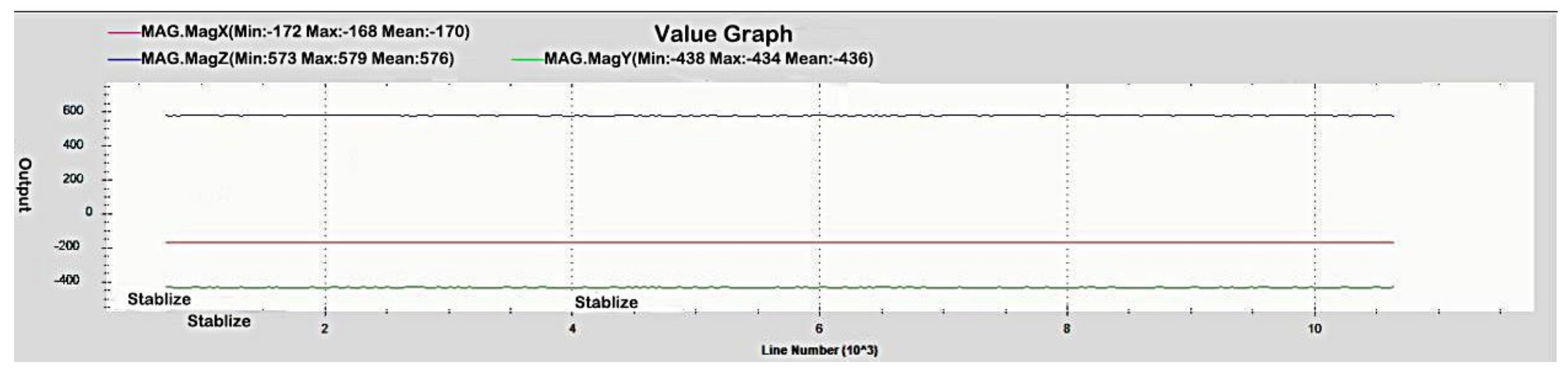
Figure 3.
The magnetic field was small, and the UAV was placed in a place where the magnetic field was normal and there was no electromagnetic or magnetic interference around it. This is the graph of the magnetometer data collected at this time. The curve in the graph is the sampling point curve, where the unit of the vertical axis is degree.

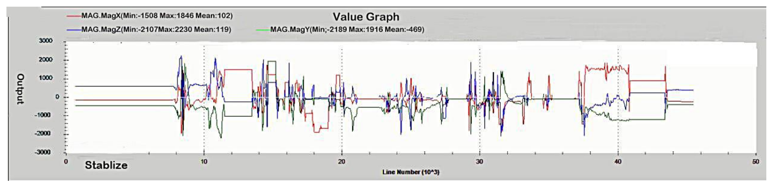
Figure 4.
The interference of magnetic field was large, and the UAV was placed in the normal magnetic field environment. A magnet with Gauss on the surface of 0.3 (Tesla) was held. The magnet was close to the UAV, making the environment one of strong magnetic field interference. This is the graph of the magnetometer data collected at this time. The curve in the graph is the sampling point curve, where the unit of the vertical axis is degree. And we can see the sampling data fluctuates greatly.

Figure 5.
The curve of course angle of UAV under test condition 1. The curve in the graph is the sampling point curve, where the unit of the vertical axis is degree. The green line is the expected value of the heading angle, and the red line is the heading angle calculated by the magnetometer. The amplitude of the course is 0.8 degrees.

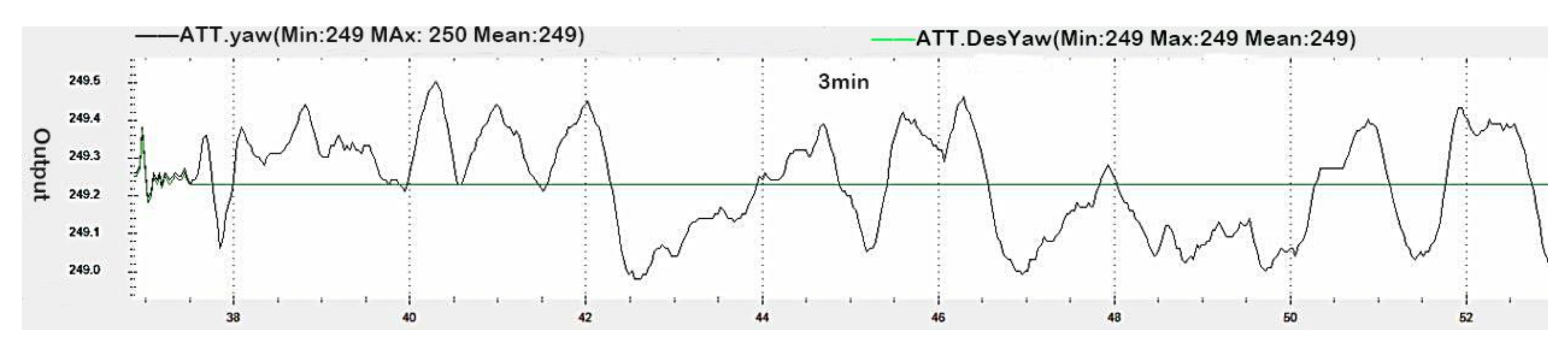
Figure 6.
The curve of course angle of UAV under test condition 2. The curve in the graph is the sampling point curve, where the unit of the vertical axis is degree. The green line is the expected value of the heading angle, and the red line is the heading angle calculated by the dual antenna. The amplitude of the course is 0.5 degrees.

Figure 7.
The curve of UAV’s course angle fluctuation under test condition 3. The curve in the graph is the sampling point curve, where the unit of the vertical coordinate is degree. The green line is the expected value of the heading angle, and the red line is the heading angle calculated by the UAV magnetometer, with a fluctuation range of 5.7 degrees.

Figure 8.
The angle fluctuation curve of the UAV under test condition 4. The curve in the graph is the sampling point curve, where the unit of the vertical coordinate is degree. The green line is the expected value, the red line is the unmanned aerial vehicle dual antenna to calculate the direction angle, the fluctuation amplitude is small, and it is 0.3 degrees.


Table 1.
We conducted four experiments in two different experimental conditions to test the dual antenna UAV antimagnetic interference ability. The experimental conditions have been explained in Section 4. The greater the amplitude of fluctuation, the poorer the UAV anti-magnetic-interference ability.
| Test Condition | Expected Value | Maximum Calculation | Minimum Calculation | Amplitude of Fluctuation |
|---|---|---|---|---|
| Test condition 1 | 135.68° | 136.1° | 135.3° | 0.8° |
| Test condition 2 | 249.23° | 249.5° | 249° | 0.5° |
| Test condition 3 | 154.2° | 166° | 154.3° | 5.7° |
| Test condition 4 | 238.9° | 240.02° | 239.72 | 0.3° |
© 2018 by the authors. Licensee MDPI, Basel, Switzerland. This article is an open access article distributed under the terms and conditions of the Creative Commons Attribution (CC BY) license (http://creativecommons.org/licenses/by/4.0/).
Share and Cite
MDPI and ACS Style
Zhai, Y.; Zhao, H.; Zhao, M.; Jiao, S. Design of Electric Patrol UAVs Based on a Dual Antenna System. Energies 2018, 11, 866. https://doi.org/10.3390/en11040866
AMA Style
Zhai Y, Zhao H, Zhao M, Jiao S. Design of Electric Patrol UAVs Based on a Dual Antenna System. Energies. 2018; 11(4):866. https://doi.org/10.3390/en11040866
Chicago/Turabian StyleZhai, Yongjie, Hailong Zhao, Meng Zhao, and Songming Jiao. 2018. "Design of Electric Patrol UAVs Based on a Dual Antenna System" Energies 11, no. 4: 866. https://doi.org/10.3390/en11040866
Note that from the first issue of 2016, this journal uses article numbers instead of page numbers. See further details here.