Evaluation of SMOS, SMAP, ASCAT and Sentinel-1 Soil Moisture Products at Sites in Southwestern France

 , , , , , and
Abstract
:
1. Introduction
2. Dataset Description
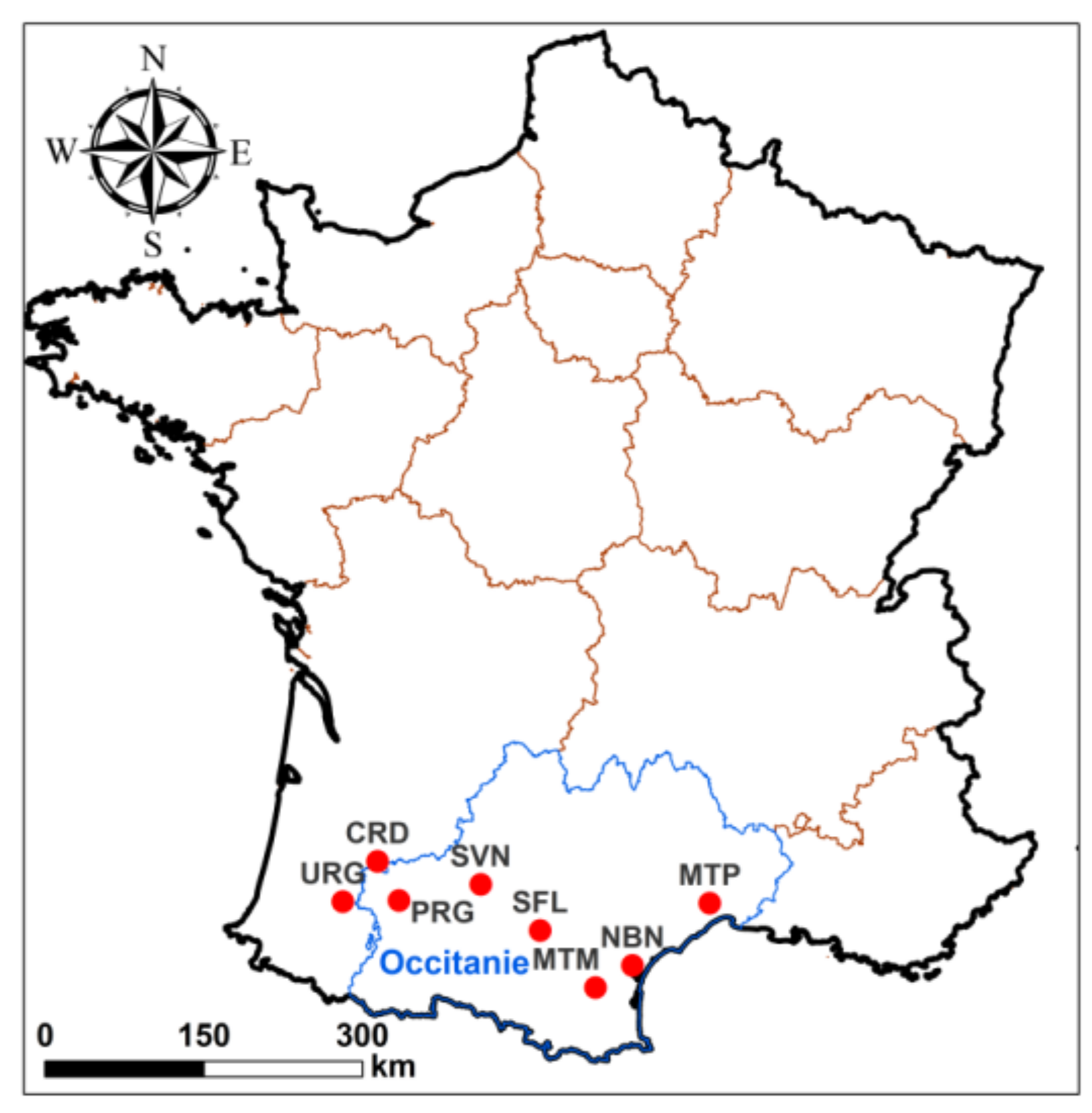
2.1. In Situ Soil Moisture Measurements
2.2. SMOS-Centre Aval de Traitement des Données SMOS Level 3 product
2.3. SMOS Near-Real-Time Product
2.4. SMOS INRA-CESBIO Product
2.5. Soil Moisture Active Passive Products
2.6. Advanced Scatterometer Products
2.7. Sentinel-1 Products
3. Results
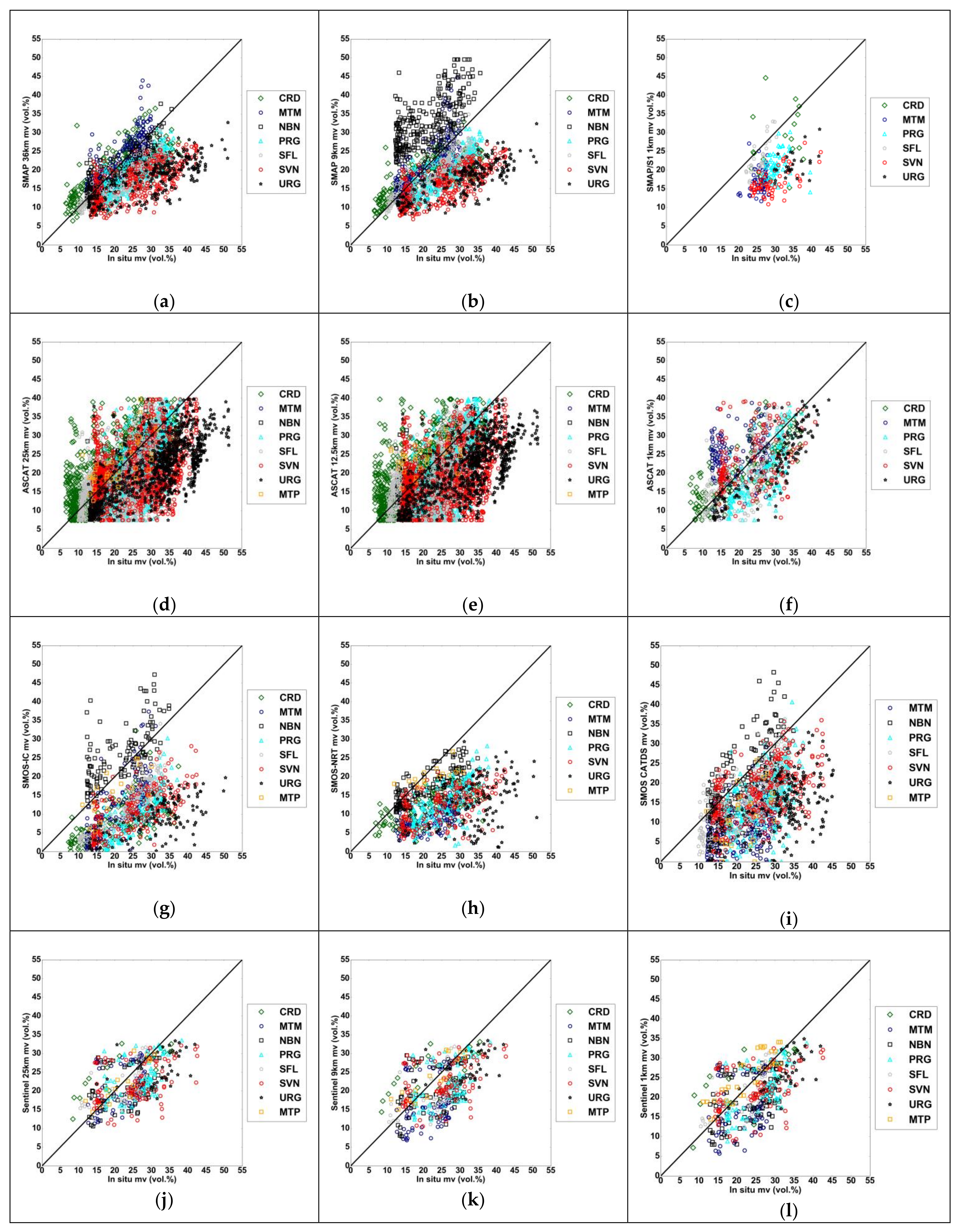
3.1. Using Together All the Data of All the Stations
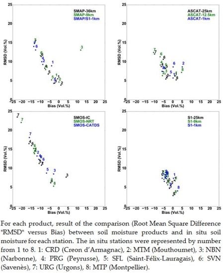
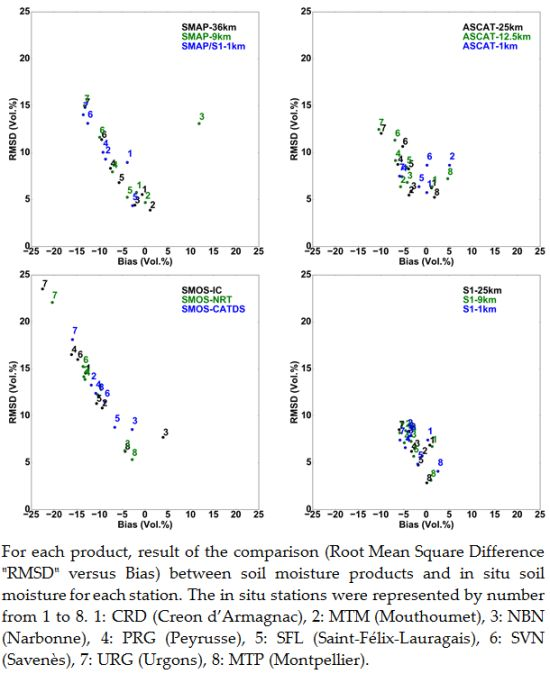
3.2. Using Each Station Alone and the Station Average of Statistics
4. Discussion
5. Conclusions
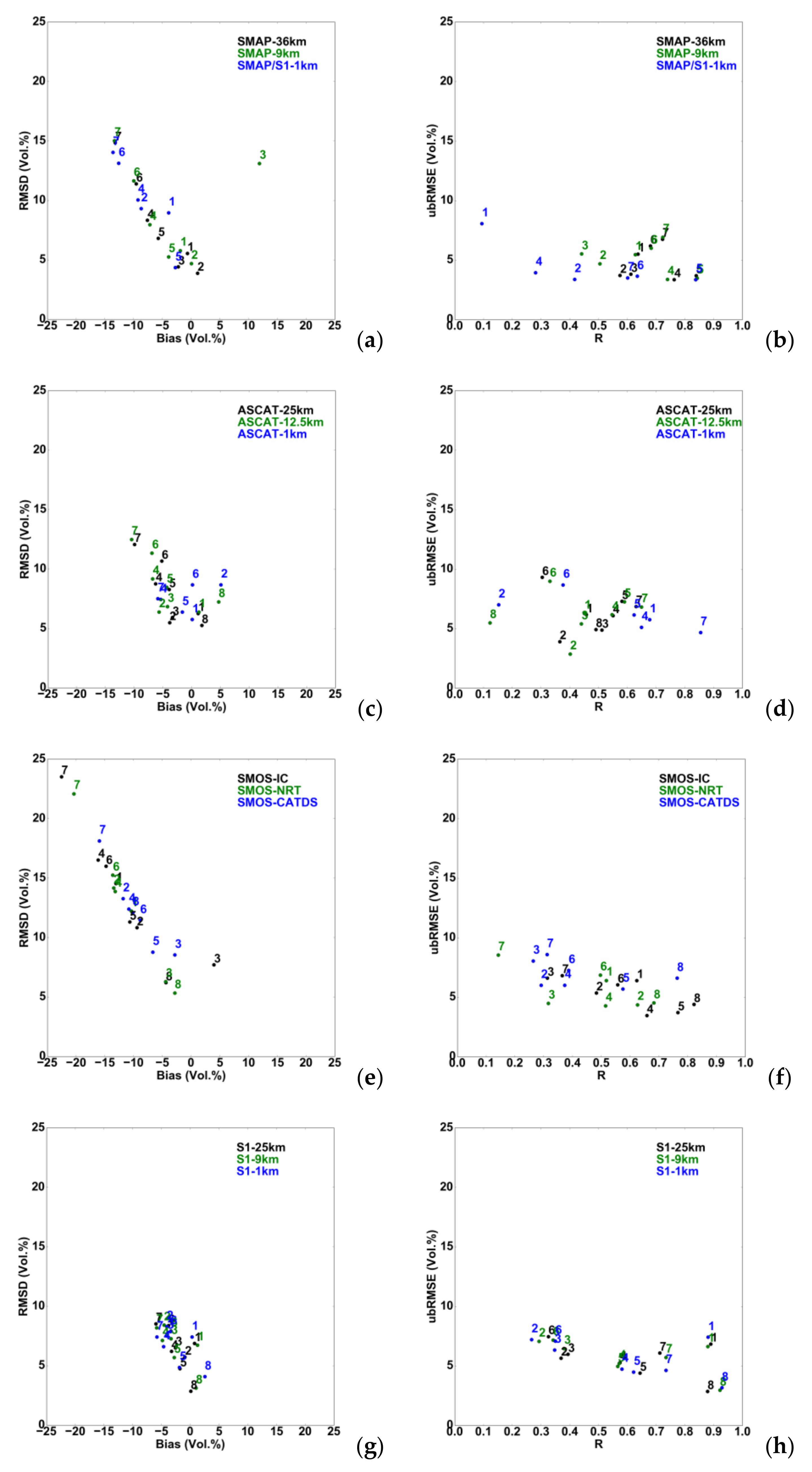
- (i)
- the SMAP/S1-1 km has lower accuracy than SMAP-36 km and SMAP-9 km,
- (ii)
- the accuracy of SMAP-36 km and SMAP-9 km (station average bias about −4.5 vol. %, and station average RMSD about 8.5 vol. %) was better than that of SMOS products (SMOS-IC, SMOS-NRT, and SMOS-CATDS) (station average bias about −10.6 vol. %, and station average RMSD about 12.7 vol. %). On our study sites, this could be related to the presence of RFI noise that affects more SMOS brightness temperature measurements,
- (iii)
- the accuracy of SMAP products (SMAP-36 km and SMAP-9 km) was close to that of ASCAT (ASCAT-25 km, ASCAT-12.5 km and ASCAT-1 km) and S1 (S1-25 km, S1-9 km, and S1-1 km) products.
Acknowledgments
Author Contributions
Conflicts of Interest
References
- Huntington, T.G. Evidence for intensification of the global water cycle: Review and synthesis. J. Hydrol. 2006, 319, 83–95. [Google Scholar] [CrossRef]
- Daly, E.; Porporato, A. A review of soil moisture dynamics: From rainfall infiltration to ecosystem response. Environ. Eng. Sci. 2005, 22, 9–24. [Google Scholar] [CrossRef]
- Koster, R.D.; Dirmeyer, P.A.; Guo, Z.; Bonan, G.; Chan, E.; Cox, P.; Gordon, C.T.; Kanae, S.; Kowalczyk, E.; Lawrence, D.; et al. Regions of strong coupling between soil moisture and precipitation. Science 2004, 305, 1138–1140. [Google Scholar] [CrossRef] [PubMed]
- Western, A.W.; Grayson, R.B.; Blöschl, G. Scaling of soil moisture: A hydrologic perspective. Annu. Rev. Earth Planet. Sci. 2002, 30, 149–180. [Google Scholar] [CrossRef]
- Saux-Picart, S.; Ottlé, C.; Decharme, B.; André, C.; Zribi, M.; Perrier, A.; Coudert, B.; Boulain, N.; Cappelaere, B.; Descroix, L.; et al. Water and energy budgets simulation over the AMMA-Niger super-site spatially constrained with remote sensing data. J. Hydrol. 2009, 375, 287–295. [Google Scholar] [CrossRef]
- Paris Anguela, T.; Zribi, M.; Hasenauer, S.; Habets, F.; Loumagne, C. Analysis of surface and root-zone soil moisture dynamics with ERS scatterometer and the hydrometeorological model SAFRAN-ISBA-MODCOU at Grand Morin watershed (France). Hydrol. Earth Syst. Sci. 2008, 12, 1415–1424. [Google Scholar] [CrossRef] [Green Version]
- Kerr, Y.H.; Waldteufel, P.; Wigneron, J.-P.; Delwart, S.; Cabot, F.; Boutin, J.; Escorihuela, M.-J.; Font, J.; Reul, N.; Gruhier, C.; et al. The SMOS mission: New tool for monitoring key elements ofthe global water cycle. Proc. IEEE 2010, 98, 666–687. [Google Scholar] [CrossRef] [Green Version]
- Kerr, Y.H.; Waldteufel, P.; Wigneron, J.-P.; Martinuzzi, J.-M.; Font, J.; Berger, M. Soil moisture retrieval from space: The Soil Moisture and Ocean Salinity (SMOS) mission. IEEE Trans. Geosci. Remote Sens. 2001, 39, 1729–1735. [Google Scholar] [CrossRef]
- Entekhabi, D.; Njoku, E.G.; Neill, P.E.; Kellogg, K.H.; Crow, W.T.; Edelstein, W.N.; Entin, J.K.; Goodman, S.D.; Jackson, T.J.; Johnson, J.; et al. The soil moisture active passive (SMAP) mission. Proc. IEEE 2010, 98, 704–716. [Google Scholar] [CrossRef]
- Wagner, W.; Hahn, S.; Kidd, R.; Melzer, T.; Bartalis, Z.; Hasenauer, S.; Figa-Saldaña, J.; de Rosnay, P.; Jann, A.; Schneider, S.; et al. The ASCAT soil moisture product: A review of its specifications, validation results, and emerging applications. Meteorol. Z. 2013, 22, 5–33. [Google Scholar] [CrossRef]
- El Hajj, M.; Baghdadi, N.; Zribi, M.; Bazzi, H. Synergic use of Sentinel-1 and Sentinel-2 images for operational soil moisture mapping at high spatial resolution over agricultural areas. Remote Sens. 2017, 9, 1292. [Google Scholar] [CrossRef]
- Oliva, R.; Daganzo, E.; Kerr, Y.H.; Mecklenburg, S.; Nieto, S.; Richaume, P.; Gruhier, C. SMOS radio frequency interference scenario: Status and actions taken to improve the RFI environment in the 1400–1427-MHz passive band. IEEE Trans. Geosci. Remote Sens. 2012, 50, 1427–1439. [Google Scholar] [CrossRef] [Green Version]
- Scipal, K.; Drusch, M.; Wagner, W. Assimilation of a ERS scatterometer derived soil moisture index in the ECMWF numerical weather prediction system. Adv. Water Resour. 2008, 31, 1101–1112. [Google Scholar] [CrossRef]
- Naeimi, V.; Paulik, C.; Bartsch, A.; Wagner, W.; Kidd, R.; Park, S.-E.; Elger, K.; Boike, J. ASCAT Surface State Flag (SSF): Extracting information on surface freeze/thaw conditions from backscatter data using an empirical threshold-analysis algorithm. IEEE Trans. Geosci. Remote Sens. 2012, 50, 2566–2582. [Google Scholar] [CrossRef]
- Al Bitar, A.; Leroux, D.; Kerr, Y.H.; Merlin, O.; Richaume, P.; Sahoo, A.; Wood, E.F. Evaluation of SMOS soil moisture products over continental US using the SCAN/SNOTEL network. IEEE Trans. Geosci. Remote Sens. 2012, 50, 1572–1586. [Google Scholar] [CrossRef] [Green Version]
- Albergel, C.; Rüdiger, C.; Carrer, D.; Calvet, J.-C.; Fritz, N.; Naeimi, V.; Bartalis, Z.; Hasenauer, S. An evaluation of ASCAT surface soil moisture products with in-situ observations in Southwestern France. Hydrol. Earth Syst. Sci. 2009, 13, 115–124. [Google Scholar] [CrossRef]
- Albergel, C.; De Rosnay, P.; Gruhier, C.; Muñoz-Sabater, J.; Hasenauer, S.; Isaksen, L.; Kerr, Y.; Wagner, W. Evaluation of remotely sensed and modelled soil moisture products using global ground-based in situ observations. Remote Sens. Environ. 2012, 118, 215–226. [Google Scholar] [CrossRef]
- Brocca, L.; Hasenauer, S.; Lacava, T.; Melone, F.; Moramarco, T.; Wagner, W.; Dorigo, W.; Matgen, P.; Martínez-Fernández, J.; Llorens, P.; et al. Soil moisture estimation through ASCAT and AMSR-E sensors: An intercomparison and validation study across Europe. Remote Sens. Environ. 2011, 115, 3390–3408. [Google Scholar] [CrossRef]
- Leroux, D.J.; Kerr, Y.H.; Richaume, P.; Berthelot, B. Estimating SMOS error structure using triple collocation. In Proceedings of the 2011 IEEE International Geoscience and Remote Sensing Symposium (IGARSS), Vancouver, BC, Canada, 24–29 July 2011; pp. 24–27. [Google Scholar]
- Sanchez, N.; Martínez-Fernández, J.; Scaini, A.; Perez-Gutierrez, C. Validation of the SMOS L2 soil moisture data in the REMEDHUS network (Spain). IEEE Trans. Geosci. Remote Sens. 2012, 50, 1602–1611. [Google Scholar] [CrossRef]
- Sinclair, S.; Pegram, G.G.S. A comparison of ASCAT and modelled soil moisture over South Africa, using TOPKAPI in land surface mode. Hydrol. Earth Syst. Sci. 2010, 14, 613–626. [Google Scholar] [CrossRef]
- Su, Z.; Wen, J.; Dente, L.; van der Velde, R.; Wang, L.; Ma, Y.; Yang, K.; Hu, Z. A plateau scale soil moisture and soil temperature observatory for quantifying uncertainties in coarse resolution satellite products. Hydrol. Earth Syst. Sci. Discuss. 2011, 8, 243–276. [Google Scholar] [CrossRef]
- Al-Yaari, A.; Wigneron, J.-P.; Ducharne, A.; Kerr, Y.H.; Wagner, W.; De Lannoy, G.; Reichle, R.; Al Bitar, A.; Dorigo, W.; Richaume, P.; et al. Global-scale comparison of passive (SMOS) and active (ASCAT) satellite based microwave soil moisture retrievals with soil moisture simulations (MERRA-Land). Remote Sens. Environ. 2014, 152, 614–626. [Google Scholar] [CrossRef] [Green Version]
- Parrens, M.; Zakharova, E.; Lafont, S.; Calvet, J.-C.; Kerr, Y.; Wagner, W.; Wigneron, J.-P. Comparing soil moisture retrievals from SMOS and ASCAT over France. Hydrol. Earth Syst. Sci. 2012, 16, 423–440. [Google Scholar] [CrossRef]
- Jackson, T.J.; Cosh, M.H.; Bindlish, R.; Starks, P.J.; Bosch, D.D.; Seyfried, M.; Goodrich, D.C.; Moran, M.S.; Du, J. Validation of advanced microwave scanning radiometer soil moisture products. IEEE Trans. Geosci. Remote Sens. 2010, 48, 4256–4272. [Google Scholar] [CrossRef]
- Jackson, T.J.; Bindlish, R.; Cosh, M.H.; Zhao, T.; Starks, P.J.; Bosch, D.D.; Seyfried, M.; Moran, M.S.; Goodrich, D.C.; Kerr, Y.H.; et al. Validation of soil moisture and ocean salinity (SMOS) soil moisture over watershed networks in the US. IEEE Trans. Geosci. Remote Sens. 2012, 50, 1530–1543. [Google Scholar] [CrossRef] [Green Version]
- Colliander, A.; Jackson, T.J.; Bindlish, R.; Chan, S.; Das, N.; Kim, S.B.; Cosh, M.H.; Dunbar, R.S.; Dang, L.; Pashaian, L.; et al. Validation of SMAP surface soil moisture products with core validation sites. Remote Sens. Environ. 2017, 191, 215–231. [Google Scholar] [CrossRef]
- Calvet, J.-C.; Fritz, N.; Froissard, F.; Suquia, D.; Petitpa, A.; Piguet, B. In situ soil moisture observations for the CAL/VAL of SMOS: The SMOSMANIA network. In Proceedings of the IEEE International Geoscience and Remote Sensing Symposium, IGARSS 2007, Barcelona, Spain, 23–28 July 2007; pp. 1196–1199. [Google Scholar]
- Albergel, C.; Rüdiger, C.; Pellarin, T.; Calvet, J.-C.; Fritz, N.; Froissard, F.; Suquia, D.; Petitpa, A.; Piguet, B.; Martin, E. From near-surface to root-zone soil moisture using an exponential filter: An assessment of the method based on in-situ observations and model simulations. Hydrol. Earth Syst. Sci. Discuss. 2008, 12, 1323–1337. [Google Scholar] [CrossRef]
- Albergel, C.; Calvet, J.-C.; De Rosnay, P.; Balsamo, G.; Wagner, W.; Hasenauer, S.; Naeimi, V.; Martin, E.; Bazile, E.; Bouyssel, F.; et al. Cross-evaluation of modelled and remotely sensed surface soil moisture with in situ data in southwestern France. Hydrol. Earth Syst. Sci. 2010, 14, 2177–2191. [Google Scholar] [CrossRef] [Green Version]
- Al Bitar, A.; Mialon, A.; Kerr, Y.H.; Cabot, F.; Richaume, P.; Jacquette, E.; Quesney, A.; Mahmoodi, A.; Tarot, S.; Parrens, M.; et al. The global SMOS Level 3 daily soil moisture and brightness temperature maps. Earth Syst. Sci. Data 2017, 9, 293–315. [Google Scholar] [CrossRef]
- Brodzik, M.J.; Billingsley, B.; Haran, T.; Raup, B.; Savoie, M.H. EASE-Grid 2.0: Incremental but significant improvements for Earth-gridded data sets. ISPRS Int. J. Geo-Inf. 2012, 1, 32–45. [Google Scholar] [CrossRef]
- Wigneron, J.-P.; Kerr, Y.; Waldteufel, P.; Saleh, K.; Escorihuela, M.-J.; Richaume, P.; Ferrazzoli, P.; De Rosnay, P.; Gurney, R.; Calvet, J.-C.; et al. L-band microwave emission of the biosphere (L-MEB) model: Description and calibration against experimental data sets over crop fields. Remote Sens. Environ. 2007, 107, 639–655. [Google Scholar] [CrossRef]
- Rodríguez-Fernández, N.J.; Sabater, J.M.; Richaume, P.; de Rosnay, P.; Kerr, Y.H.; Albergel, C.; Drusch, M.; Mecklenburg, S. SMOS near-real-time soil moisture product: Processor overview and first validation results. Hydrol. Earth Syst. Sci. 2017, 21, 5201–5216. [Google Scholar] [CrossRef]
- Kerr, Y.H.; Waldteufel, P.; Richaume, P.; Wigneron, J.P.; Ferrazzoli, P.; Mahmoodi, A.; Al Bitar, A.; Cabot, F.; Gruhier, C.; Juglea, S.E.; et al. The SMOS soil moisture retrieval algorithm. IEEE Trans. Geosci. Remote Sens. 2012, 50, 1384–1403. [Google Scholar] [CrossRef]
- Schaefer, G.L.; Cosh, M.H.; Jackson, T.J. The USDA natural resources conservation service soil climate analysis network (SCAN). J. Atmos. Ocean. Technol. 2007, 24, 2073–2077. [Google Scholar] [CrossRef]
- Bell, J.E.; Palecki, M.A.; Baker, C.B.; Collins, W.G.; Lawrimore, J.H.; Leeper, R.D.; Hall, M.E.; Kochendorfer, J.; Meyers, T.P.; Wilson, T.; et al. US Climate Reference Network soil moisture and temperature observations. J. Hydrometeorol. 2013, 14, 977–988. [Google Scholar] [CrossRef]
- Wigneron, J.P.; Mialon, A.; De Lannoy, G.; Fernandez-Moran, R.; Al-Yaari, A.; Rodriguez-Fernandez, N.; Kerr, Y.; Quets, J.; Pellarin, T.; Fan, L.; et al. SMOS-IC: Current status and overview of soil moisture and VOD applications. In Proceedings of the IEEE IGARSS, Valencia, Spain, 23–27 July 2018. submitted for publication. [Google Scholar]
- Fernandez-Moran, R.; Al-Yaari, A.; Mialon, A.; Mahmoodi, A.; Al Bitar, A.; De Lannoy, G.; Rodriguez-Fernandez, N.; Lopez-Baeza, E.; Kerr, Y.; Wigneron, J.-P. SMOS-IC: An alternative SMOS soil moisture and vegetation optical depth product. Remote Sens. 2017, 9, 457. [Google Scholar] [CrossRef]
- Fernandez-Moran, R.; Wigneron, J.-P.; De Lannoy, G.; Lopez-Baeza, E.; Parrens, M.; Mialon, A.; Mahmoodi, A.; Al-Yaari, A.; Bircher, S.; Al Bitar, A.; et al. A new calibration of the effective scattering albedo and soil roughness parameters in the SMOS SM retrieval algorithm. Int. J. Appl. Earth Obs. Geoinf. 2017, 62, 27–38. [Google Scholar] [CrossRef]
- O’Neill, P.E.; Njoku, E.G.; Jackson, T.J.; Chan, S.; Bindlish, R. SMAP Algorithm Theoretical Basis Document: level 2 & 3 Soil Moisture (Passive) Data Products; JPL D-66480; Jet Propuls. Lab., California Inst. Technol.: Pasadena, CA, USA, 2015. [Google Scholar]
- Jackson, T.J.; Schmugge, T.J. Vegetation effects on the microwave emission of soils. Remote Sens. Environ. 1991, 36, 203–212. [Google Scholar] [CrossRef]
- Kim, H.; Parinussa, R.; Konings, A.; Wagner, W.; Cosh, M.; Choi, M. Global-scale Assessment and Combination of SMAP with ASCAT (Active) and AMSR2 (Passive) Soil Moisture Products. EGU Gen. Assem. Conf. Abstr. 2018, 19, 10957. [Google Scholar] [CrossRef]
- Naeimi, V.; Bartalis, Z.; Wagner, W. ASCAT soil moisture: An assessment of the data quality and consistency with the ERS scatterometer heritage. J. Hydrometeorol. 2009, 10, 555–563. [Google Scholar] [CrossRef]
- Naeimi, V.; Scipal, K.; Bartalis, Z.; Hasenauer, S.; Wagner, W. An improved soil moisture retrieval algorithm for ERS and METOP scatterometer observations. IEEE Trans. Geosci. Remote Sens. 2009, 47, 1999–2013. [Google Scholar] [CrossRef]
- Wagner, W.; Noll, J.; Borgeaud, M.; Rott, H. Monitoring soil moisture over the Canadian prairies with the ERS scatterometer. Geosci. IEEE Trans. Remote Sens. 1999, 37, 206–216. [Google Scholar] [CrossRef]
- Amri, R.; Zribi, M.; Lili-Chabaane, Z.; Wagner, W.; Hasenauer, S. Analysis of C-band scatterometer moisture estimations derived over a semiarid region. IEEE Trans. Geosci. Remote Sens. 2012, 50, 2630–2638. [Google Scholar] [CrossRef]
- Draper, C.S.; Reichle, R.H.; De Lannoy, G.J.M.; Liu, Q. Assimilation of passive and active microwave soil moisture retrievals. Geophys. Res. Lett. 2012, 39. [Google Scholar] [CrossRef] [Green Version]
- Inglada, J.; Vincent, A.; Arias, M.; Tardy, B.; Morin, D.; Rodes, I. Operational high resolution land cover map production at the country scale using satellite image time series. Remote Sens. 2017, 9, 95. [Google Scholar] [CrossRef]
- Attema, E.P.W.; Ulaby, F.T. Vegetation modeled as a water cloud. Radio Sci. 1978, 13, 357–364. [Google Scholar] [CrossRef]
- Fung, A.K. Microwave Scattering and Emission Models and Their Applications; Artech House: Boston, MA, USA, 1994; ISBN 978-0-89006-523-5. [Google Scholar]
- Baghdadi, N.; El Hajj, M.; Zribi, M.; Bousbih, S. Calibration of the Water Cloud Model at C-Band for Winter Crop Fields and Grasslands. Remote Sens. 2017, 9, 969. [Google Scholar] [CrossRef]
- Baghdadi, N.; Zribi, M. Characterization of Soil Surface Properties Using Radar Remote Sensing. In Land Surface Remote Sensing in Continental Hydrology; Elsevier: Oxford, UK, 2016; pp. 1–39. [Google Scholar]
- Baghdadi, N.; Holah, N.; Zribi, M. Calibration of the integral equation model for SAR data in C-band and HH and VV polarizations. Int. J. Remote Sens. 2006, 27, 805–816. [Google Scholar] [CrossRef]
- Baghdadi, N.; Gherboudj, I.; Zribi, M.; Sahebi, M.; King, C.; Bonn, F. Semi-empirical calibration of the IEM backscattering model using radar images and moisture and roughness field measurements. Int. J. Remote Sens. 2004, 25, 3593–3623. [Google Scholar] [CrossRef]
- Baghdadi, N.; Cresson, R.; El Hajj, M.; Ludwig, R.; La Jeunesse, I. Estimation of soil parameters over bare agriculture areas from C-band polarimetric SAR data using neural networks. Hydrol. Earth Syst. Sci. 2012, 16, 1607–1621. [Google Scholar] [CrossRef] [Green Version]
- Albergel, C.; Dorigo, W.; Reichle, R.H.; Balsamo, G.; De Rosnay, P.; Muñoz-Sabater, J.; Isaksen, L.; De Jeu, R.; Wagner, W. Skill and global trend analysis of soil moisture from reanalyses and microwave remote sensing. J. Hydrometeorol. 2013, 14, 1259–1277. [Google Scholar] [CrossRef]
- Kumar, S.V.; Peters-Lidard, C.D.; Mocko, D.; Reichle, R.; Liu, Y.; Arsenault, K.R.; Xia, Y.; Ek, M.; Riggs, G.; Livneh, B.; et al. Assimilation of remotely sensed soil moisture and snow depth retrievals for drought estimation. J. Hydrometeorol. 2014, 15, 2446–2469. [Google Scholar] [CrossRef]
- Al-Yaari, A.; Wigneron, J.-P.; Kerr, Y.; Rodriguez-Fernandez, N.; O’Neill, P.E.; Jackson, T.J.; De Lannoy, G.J.M.; Al Bitar, A.; Mialon, A.; Richaume, P.; et al. Evaluating soil moisture retrievals from ESA’s SMOS and NASA’s SMAP brightness temperature datasets. Remote Sens. Environ. 2017, 193, 257–273. [Google Scholar] [CrossRef]
- Delwart, S.; Bouzinac, C.; Wursteisen, P.; Berger, M.; Drinkwater, M.; Martín-Neira, M.; Kerr, Y.H. SMOS validation and the COSMOS campaigns. IEEE Trans. Geosci. Remote Sens. 2008, 46, 695–704. [Google Scholar] [CrossRef]
- Kerr, Y.H.; Al-Yaari, A.; Rodriguez-Fernandez, N.; Parrens, M.; Molero, B.; Leroux, D.; Bircher, S.; Mahmoodi, A.; Mialon, A.; Richaume, P.; et al. Overview of SMOS performance in terms of global soil moisture monitoring after six years in operation. Remote Sens. Environ. 2016, 180, 40–63. [Google Scholar] [CrossRef]


| Products | Bias (vol. %) | RMSD (vol. %) | ubRMSD (vol. %) | R | N |
|---|---|---|---|---|---|
| SMAP-36 km | −5.5/−5.4 | 8.7/7.9 | 6.8/4.7 | 0.69/0.69 | 1847 |
| SMAP-9 km | −3.5/−3.5 | 9.8/9.1 | 9.2/5.1 | 0.66/0.65 | 1793 |
| SMAP/S1-1 km | −9.2/−8.5 | 10.6/10.0 | 5.4/4.3 | 0.48/0.48 | 259 |
| ASCAT-25 km | −4.7/−3.7 | 9.1/7.8 | 7.9/6.2 | 0.50/0.49 | 5291 |
| ASCAT-12.5 km | −5.2/−4.1 | 9.4/8.5 | 7.8/6.1 | 0.50/0.44 | 5252 |
| ASCAT-1 km | −1.2/−1.3 | 7.5/7.4 | 7.4/6.2 | 0.55/0.56 | 942 |
| SMOS-IC | −11.9/−10.9 | 14.8/13.3 | 8.7/5.3 | 0.56/0.57 | 1128 |
| SMOS-NRT | −12.4/−11.2 | 14.5/12.7 | 7.6/5.6 | 0.43/0.47 | 900 |
| SMOS-CATDS | −9.5/−9.6 | 12.3/12.1 | 7.8/6.9 | 0.38/0.42 | 1479 |
| S1-25 km | −2.6/−2.2 | 6.7/6.2 | 6.1/5.6 | 0.49/0.60 | 459 |
| S1-9 km | −3.7/−2.8 | 7.4/6.8 | 6.5/5.8 | 0.48/0.59 | 447 |
| S1-1 km | −3.45/−2.6 | 7.2/6.8 | 6.3/5.6 | 0.50/0.59 | 462 |
© 2018 by the authors. Licensee MDPI, Basel, Switzerland. This article is an open access article distributed under the terms and conditions of the Creative Commons Attribution (CC BY) license (http://creativecommons.org/licenses/by/4.0/).
Share and Cite
El Hajj, M.; Baghdadi, N.; Zribi, M.; Rodríguez-Fernández, N.; Wigneron, J.P.; Al-Yaari, A.; Al Bitar, A.; Albergel, C.; Calvet, J.-C. Evaluation of SMOS, SMAP, ASCAT and Sentinel-1 Soil Moisture Products at Sites in Southwestern France. Remote Sens. 2018, 10, 569. https://doi.org/10.3390/rs10040569
El Hajj M, Baghdadi N, Zribi M, Rodríguez-Fernández N, Wigneron JP, Al-Yaari A, Al Bitar A, Albergel C, Calvet J-C. Evaluation of SMOS, SMAP, ASCAT and Sentinel-1 Soil Moisture Products at Sites in Southwestern France. Remote Sensing. 2018; 10(4):569. https://doi.org/10.3390/rs10040569
Chicago/Turabian StyleEl Hajj, Mohammad, Nicolas Baghdadi, Mehrez Zribi, Nemesio Rodríguez-Fernández, Jean Pierre Wigneron, Amen Al-Yaari, Ahmad Al Bitar, Clément Albergel, and Jean-Christophe Calvet. 2018. "Evaluation of SMOS, SMAP, ASCAT and Sentinel-1 Soil Moisture Products at Sites in Southwestern France" Remote Sensing 10, no. 4: 569. https://doi.org/10.3390/rs10040569