Electricity Consumption Clustering Using Smart Meter Data

1
Systems Analysis, the Department of Management Engineering, Technical University of Denmark, 2800 Kgs. Lyngby 2800 Kgs, Denmark
2
Dynamical Systems, the Department Compute, Technical University of Denmark, 2800 Kgs. Lyngby 2800 Kgs, Denmark
*
Author to whom correspondence should be addressed.
Energies 2018, 11(4), 859; https://doi.org/10.3390/en11040859
Submission received: 23 February 2018
/
Revised: 28 March 2018
/
Accepted: 4 April 2018
/
Published: 6 April 2018
Abstract
:Electricity smart meter consumption data is enabling utilities to analyze consumption information at unprecedented granularity. Much focus has been directed towards consumption clustering for diversifying tariffs; through modern clustering methods, cluster analyses have been performed. However, the clusters developed exhibit a large variation with resulting shadow clusters, making it impossible to truly identify the individual clusters. Using clearly defined dwelling types, this paper will present methods to improve clustering by harvesting inherent structure from the smart meter data. This paper clusters domestic electricity consumption using smart meter data from the Danish city of Esbjerg. Methods from time series analysis and wavelets are applied to enable the K-Means clustering method to account for autocorrelation in data and thereby improve the clustering performance. The results show the importance of data knowledge and we identify sub-clusters of consumption within the dwelling types and enable K-Means to produce satisfactory clustering by accounting for a temporal component. Furthermore our study shows that careful preprocessing of the data to account for intrinsic structure enables better clustering performance by the K-Means method.
1. Introduction
The number of days that Denmark fully covers its electricity demand through renewable sources is increasing. By the end of 2020, renewable electricity production in Denmark is projected to cover an average of 84% of electricity demand [1]. Though there is still a deficit of renewables in the system, the gap is closing, also at a European scale [2]. The caveat is that renewables induce volatility in the electricity grid as the production is tied to uncontrollable sources. A deeper understanding of electricity demand can help alleviate the implications of the volatile production, by promoting flexible consumption through tariff incentives.
The advent of residential electricity smart meters has enabled utilities to record and monitor electricity consumption by the minute. Recording electricity consumption at this unprecedented granularity can help us understand electricity demand in more detail. Analyzing consumption patterns can enable electricity utilities to develop targeted tariffs for individual groups mitigating production volatility by harnessing the flexibility of consumers.
The future electricity grid is expected to experience growing demand from the electrification of transportation [1] and the increased application of electric heat pumps. The introduction of renewable resources in the electricity sector therefore introduces significant challenges. The expected increase in demand and volatility in electricity production will put a strain on the entire distribution and transmission grid. Demand flexibility has been discussed as a means to match demand with the volatility in production. To evaluate demand flexibility, a deeper understanding of consumption patterns is essential.
The application of smart meter data to cluster electricity consumption is a research field that has been gaining momentum over the past decade, beginning with [3], which analyzed smart meter electricity data, clustering methods and validation. In the electricity smart meter literature, K-Means is a very prevalent [4] method for clustering. The clusters created often exhibit variation to such an extent that clusters overlap, resulting in academically viable but practically indistinguishable clusters.
This paper will apply modern data mining techniques and methods from signal analysis to reduce the cluster overlap. The proposed methods will enable K-Means to analyze intrinsic data information which was previously ignored by the clustering. Reducing the overlap will produce more distinguishable and generally applicable cluster solutions. Data from more than 34,000 household electricity smart meters are included in the analysis performed in this paper. This paper contributes to the electricity smart meter literature through the following:
- Presenting a cluster analysis of Danish household electricity consumption data.
- Confirmation of autocorrelation in the data, information which K-Means is unable to incorporate in the clustering.
- Transformation and extraction of input data features enabling K-Means to account for autocorrelation in the clustering. This can easily be extended to include other data structures.
- Extending the concept of cross-validation to unsupervised learning employing cluster validation indices resulting in variability estimates of the resulting clustering performance.
The remainder of this paper is divided into six sections. First, Section 2 describes the current state of the art of smart meter electricity consumption classification, followed by a data summary and preprocessing in Section 3. Section 4 outlines the methodology applied in this paper. In Section 5 we apply the methodology to the smart meter electricity consumption data, followed by a discussion of the results in Section 6, and Section 7 concludes with the papers contributions.
2. Literature Review
This section presents a review of the current state of the art in smart meter electricity consumption clustering. The foundation for the study is [4], which conducts a systematic review of the current state of the art in smart meter data analytics. The paper evaluates approximately 2100 unique peer-reviewed papers and presents three main finding related to clustering methods, data and cluster validation.
Several methods for clustering have been applied and the most prevalent is K-means [5,6] and derivatives such as fuzzy K-Means [7,8] and adaptive K-Means [9]. Further algorithms like hierarchical clustering [10,11], and random effect mixture models [12,13] are also popular. Many of the papers apply K-Means for baseline clustering and compare more advanced methods to this baseline [14,15,16], with inconclusive outcomes regarding the best method for clustering. Some papers make an effort to preprocess the smart meter data; popular preprocessing methods are principal component analysis and factor analysis for dimensionality reduction [17,18] and self-organizing maps for 2 Dimensional representation of the data [3,10]. All identified methods are not particularly well-suited to time series data, such as smart meter data. Consequently, the clustering methods applied to the data do not leverage the intrinsic temporal data structure hidden in the smart meter data.
Many of the papers identified in [4] fail to acknowledge smart meter readings as time series data, a data type which contains a temporal component. Only one paper recognized the time series properties through the application of Fourier transformation, which maps data from the time to the frequency domain and subsequently applies K-Means to cluster by largest frequency [7]. The omission of the time series structure in the analysis leads to the application of methods that are not designed for handling temporal components. K-Means ignores autocorrelation, unless the input data is preprocessed; methods for preprocessing input data to enable K-Means to account for autocorrelation are described in [19].
In [20,21], principal component analysis and similarity measures for time series evaluation of generic data are discussed. The conclusions are applicable to smart meter data, although the method works best with fewer meters than recordings and thus, conversely, the dataset expands.
The clusters identified in the papers are validated by a variety of indices, with the most prevalent being the cluster dispersion index (CDI) [22,23,24], the Davies–Bouldin index (DBI) [25,26] and the mean index adequacy (MIA) [8,13].
This paper will describe methods for preprocessing smart meter data to enable K-Means to evaluate autocorrelation in data. These methods will make it possible to exploit hidden structures and thus increase the amount of information applicable for clustering.
3. Data Summary and Preparation
This section introduces the smart meter electricity consumption data that will be analyzed for the remainder of this paper. The data is kindly provided by SydEnergi, the largest electricity utility company in southern Denmark.
This paper analyzes consumption patterns for apartments and (semi)detached houses connected to the district heating system in the city of Esbjerg. It covers four postal codes—6700, 6705, 6710, and 6715—and the two selected household types are expected to behave identically. There were initially 34,000+ consumers of these two types in Esbjerg, each with a smart meter installed that records consumption every 60 min. We only analyzed these two residential categories as we were interested in analyzing consumption differences within consumer groups and not across different housing types.
The literature does not advise on the time length for analyzing consumption patterns. Paper [16] analyzes load profiles with a consumption window of one week, which is also the consumption window that we selected for this study. We selected the second week of January 2011, starting on Monday the 10th and ending Sunday the 16th, with both days included. With consumption recorded each 60 min, this yields 24 recordings per day for a total of 168 recordings per meter across the seven days.
The precise number and types of smart meter data employed in this paper is described in Table 1. The accompanying waterfall table (Table 2) illustrates the effect of the preprocessing on the final data set size.
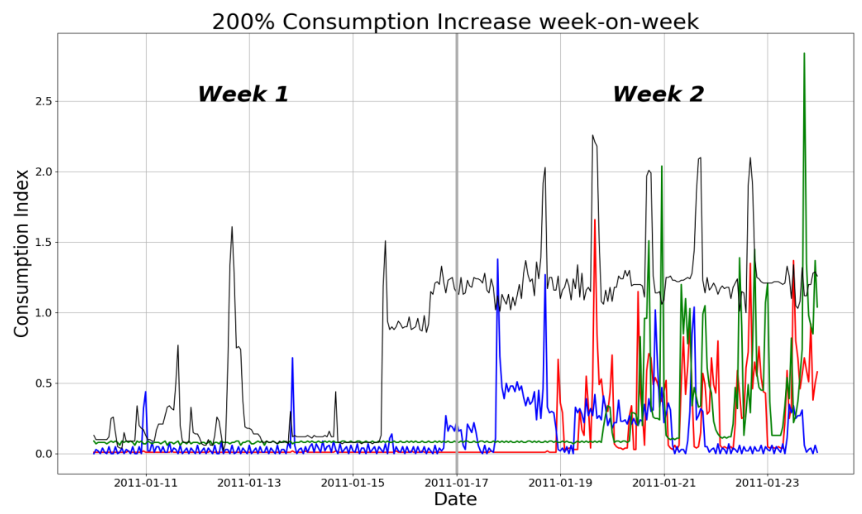
Before analysis, the data was preprocessed to remove missing data and other undesirable traits. A two-stage process for cleaning the data was applied. Stage 1 involved a simple descriptive statistical examination of the data, ensuring the removal of; missing values, zero mean consumption, zero median consumption, and zero variance, all of which would indicate missing consumption information. This preprocessing is outlined in a waterfall statistic, seen in Table 2, which presents the effect of each step of the preprocessing. For more advanced anomaly detection methods see [27]. Stage 2 exploited the fact that the data set encompassed data from the subsequent third week of January from the 17th–23rd. This helped us to identify meters that were behaving irregularly in week two, by evaluating the week-on-week consumption change. This change can be an indication of vacant dwellings with a subsequent consumption increase, e.g., returning from vacation. We defined irregular as a week-on-week consumption change of more than 200%. Meters that exhibited this consumption pattern were removed from the data set.
Figure 1 shows four different meters that exhibit week-on-week consumption changes above 200% percent. In the figure, the consumption change indicates a return to the dwelling; we were not interested in clustering vacant dwelling consumption and accordingly removed meters with a 200% increase in consumption.
4. Methodology
This section describes the theoretical statistical framework that we applied to analyze the smart meter data. Section 4.1 starts with a discussion of the concept of statistical learning and presents a flow chart illustrating the process applied in this paper. The literature review in Section 2 identified K-Means clustering as the most prevalent clustering method for electricity smart meter consumption data. Section 4.2 discusses the K-Means clustering method and the importance of normalization. Section 4.3 includes a discussion of cluster validation with the subsequent description of four selected indices—MIA, cluster dispersion index, the Davies–Bouldin index and the silhouette index. This section also includes a description of the unsupervised cross-validation applied in this paper. Section 4.4 and Section 4.5 discuss autocorrelation feature extraction and wavelet transformation, which are methods that can enable K-Means to include temporal components in the clustering process.
4.1. Statistical Learning
The statistical segmentation of data into smaller more homogeneous subsets is carried out by applying supervised or unsupervised learning. The distinction between supervised and unsupervised learning is bound to differences in the initial problem conditions. For supervised learning problems there exist some known class labels and knowledge of the membership attributes of a class. This membership knowledge is used to create a mathematical function that maps the observations to classes. For unsupervised learning, class labels do not exist. In unsupervised learning there exists no apparent external or internal information that can unambiguously identify the potential underlying clusters. Different methods have been developed in an effort to remedy the problem and enable unsupervised clustering, but the clusters identified in this way are rarely stable and unique. There exist several techniques for unsupervised clustering; popular methods include K-means and hierarchical clustering.
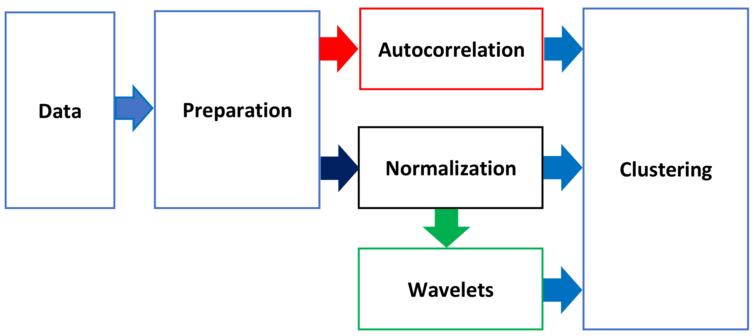
This paper introduces the extraction of data features to enable K-Means to account for the temporal component in smart meter data. Three different manipulations of the input data were investigated—normalization, wavelet transformation and autocorrelation feature extraction. Figure 2 illustrates a process overview, where blue boxes indicate the processes that all methods were subjected to. All analysis was drawn from the data, preparation of data and clustering. This paper introduces three different data manipulation methods prior to clustering, to enable K-Means to account for intrinsic information. The methods applied were autocorrelation feature extraction (red), normalization (black), and wavelets (green). We applied normalization to the wavelet transformation before clustering.
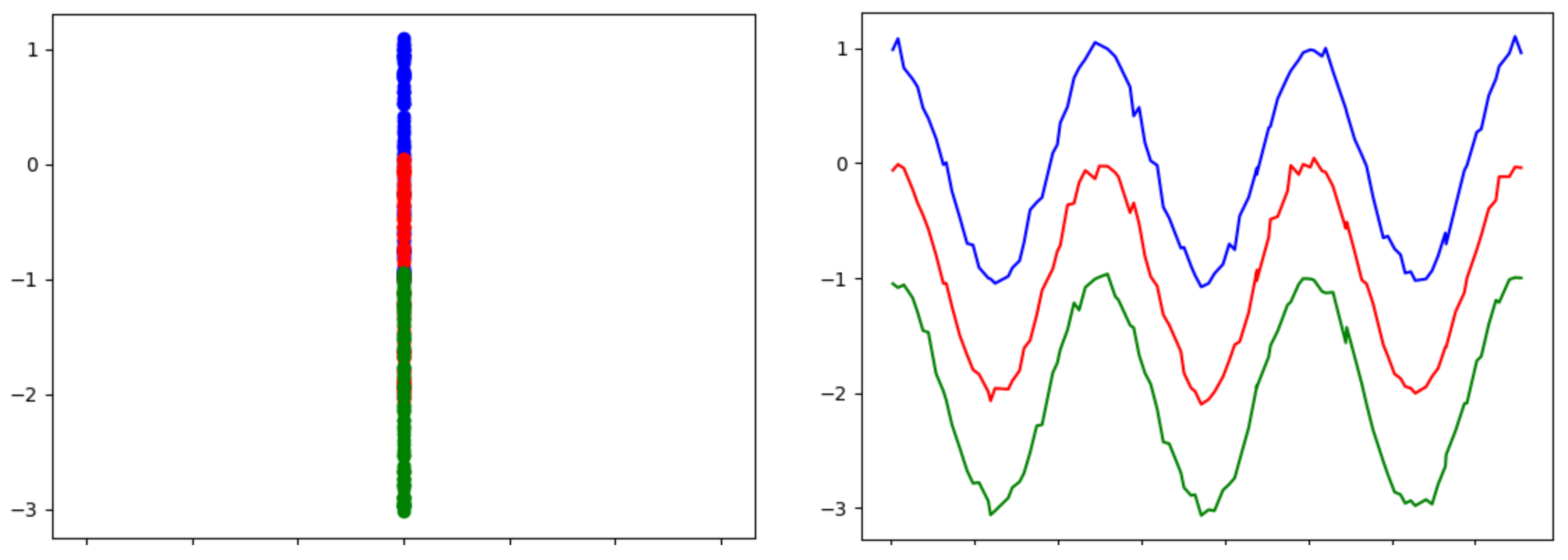
Smart meter data is recorded over time; accounting for the temporal component, which can convey information about the data patterns. By default, K-Means clustering does not consider this temporal component. Thus, a very important feature of the data—the temporal component—is not employed in the clustering. Figure 3 shows data with and without a temporal component; the left side shows data where the temporal component has been collapsed. It is not possible to estimate whether the data overlaps or is just very close in distance. The right side shows the exact same data with the temporal component reinstated. From the right side it can clearly be seen that there is a temporal structure in the data, this component reveals three different non-overlapping cosine structures. The temporal component accounts for intrinsic data information that the K-means and other unsupervised methods do not evaluate when clustering. This paper will present methods to alleviate the problem and enable the K-Means method to account for temporal structures. Preprocessing the data before clustering with K-Means can help to include the structure from the right side of Figure 3.
In electricity smart meter data analytics, the clustering methodology is often either K-Means or hierarchical clustering. These are simple and robust methods that perform reasonably well under various circumstances. Both employ a distance measure for clustering, and the selection of distance measure can heavily influence the shape of the clusters [28].
In the absence of knowledge of the true clusters, and to avoid the trivial clustering case of assigning one cluster to each observation, reducing the variability to 0, several cluster validation indices were introduced. These indices evaluated the intra-cluster distance and related it to the inter-cluster distance. Often the indices favor a clustering solution that minimizes the intra-cluster distance while maximizing the inter-cluster distance.
4.2. K-Means
As described in [4], the K-Means method is the most prevalent technique for electricity smart meter consumption clustering. K-Means is a simple and robust algorithm for partitioning n observations into k clusters. This is done by assigning each of the n observations to the closest cluster centroid given some distance measure. Due to random initialization of the K-Means algorithm, it can result in locally optimal solutions. It is advised to rerun the clustering several times with different initial random seeds and select the clustering that yields the best discriminatory performance [29].
The K-Means implementation employed in this paper is the SKlearn data analysis package for Python version 0.18.2 [30]. We used the SKlearn default settings for maximum iterations until convergence (max_iter) 300. The K-Means was by default randomly initialized 10 times. The initial random seed for testing purposes in this paper was set to 12345.
Even though K-Means yields robust solution it is important to recognize that K-Means only evaluates data from a distance perspective, which from a smart meter data perspective implies that each time step is evaluated independently without correlation to the neighboring time steps. That is; K-Means evaluates all meter readings at t = 0 without regards to any structure or correlation effect with neighboring time steps such as t = 1. Especially with time series, autocorrelation is an integral aspect, and for electricity consumption we expect there to be some recurrent structure in the consumption patterns. K-Means does not evaluate this structure, however, through feature extraction it is possible to account for the autocorrelation in the input data [19], enabling K-Means to include this information in the clustering. This paper applies both autocorrelation feature extraction and the wavelet transformation described in Section 4.4 and Section 4.5 to account for the autocorrelation.
Normalizing the smart meter time series makes the data fit the interval [0–1]; in [31], normalization was applied to smart meter data. This process makes it possible to identify time series with equivalent consumption patterns instead of identical consumption volumes. As the focus of this paper is clustering by consumption pattern, we normalize by:
4.3. Cluster Validation
In unsupervised learning there exists no natural quantification of the discrepancy between model and truth, as the true clusters are unknown. The need for evaluating the performance of unsupervised methods has resulted in the development of various cluster evaluation indices [13]. This paper has, based on the prevalence found in [4], selected four prominent indices for validation, namely MIA, the cluster dispersion index (CDI), Davies–Bouldin index (DBI) and the silhouette index. The indices each evaluate different properties of the clusters. Even though none of the indices can identify the true underlying structure, their values for different number of clusters can give an indication of how many clusters to retain in the final clustering. Plotting the progression of the indices as a function of clusters allows for visual inspection, where abrupt changes in their decline or fluctuating pattern can help select the number of clusters within a given data set [19]. We advise the evaluation of several indices jointly, as the combination can be applied to strengthen the argument for the selection of a specific number of clusters.
4.3.1. Mean Adequacy Index (MIA)
The MIA index calculates the square root of the average distance from each member of a class to the class centroid and scales it by the number of classes K.
where is the squared average distance within cluster k. The MIA index is a measure of within-class dispersion. Large distances within the class indicate a poor fit; high index values indicate large within-cluster dispersion.
4.3.2. Cluster Dispersion Index (CDI)
The CDI is a revised version the MIA index scaled by the average cluster distance . The CDI prefers large inter-cluster distances and small intra-cluster distances [24].
Smaller values indicate better clustering. d(C) is the average cluster distance between any two clusters in the clustering, while is the average squared within the cluster distance.
4.3.3. Davies–Bouldin Index (DBI)
The DBI evaluates the overlap between clusters. This is done by evaluating the average intra-cluster distance, given by of all clusters and subsequently comparing all pairs of clusters divided by their centroid distance and selecting the maximum distance for each class.
Smaller values of DBI implies that the K-means clustering algorithm separates the data set properly [11].
4.3.4. Silhouette Index
The Silhouette index evaluates the average distance between each vector within a class While is the minimum distance from a vector in class to a vector not in , scaled by the maximum distance between two classes [4].
The index is bound in the interval [−1, 1], where higher values are better; negative values indicate misclustering [31].
4.3.5. Unsupervised Cross-Validation
Cross-validation is an effort to increase model robustness by dividing the data set into a training and a test set. The training set is used to train the model and the test set is used test the model on an “unknown” data set. The process helps quantify model stability and helps reduce the chance of overfit. For cross-validation to achieve its purpose of reducing overfit and evaluating model performance, there needs to exist a measure of fit. For unsupervised learning no such fit exists [32]; to remedy this situation we regard the cluster validation indices as the measure of fit, creating a pseudo cross-validation measure for the fit of our clustering. This pseudo cross-validation enables us at each number of clusters to evaluate the maximum and minimum value of the index and thus how stable the index is for a given number of clusters. This paper applied 10-fold cross validation to the indices.
4.4. Autocorrelation Feature Extraction
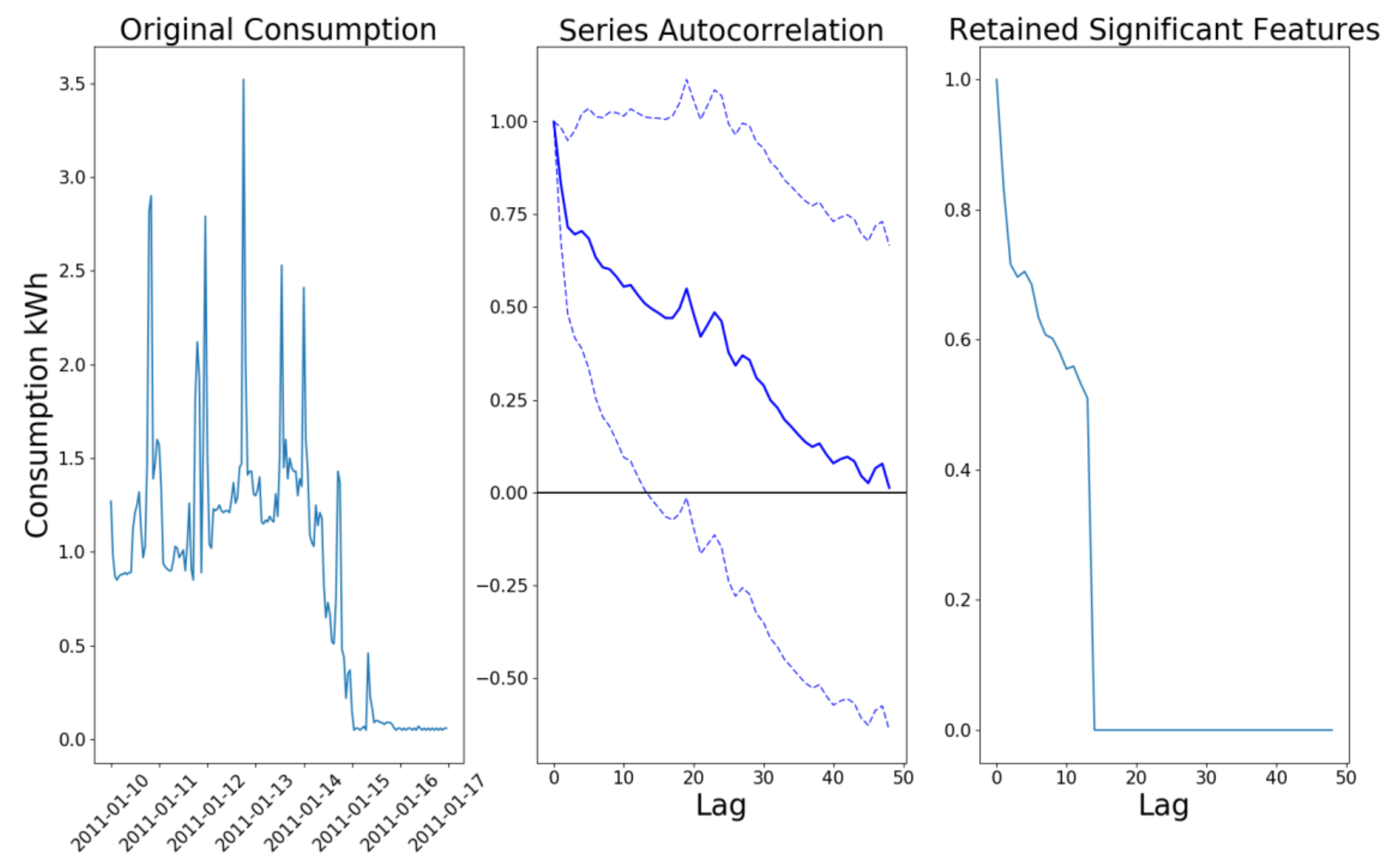
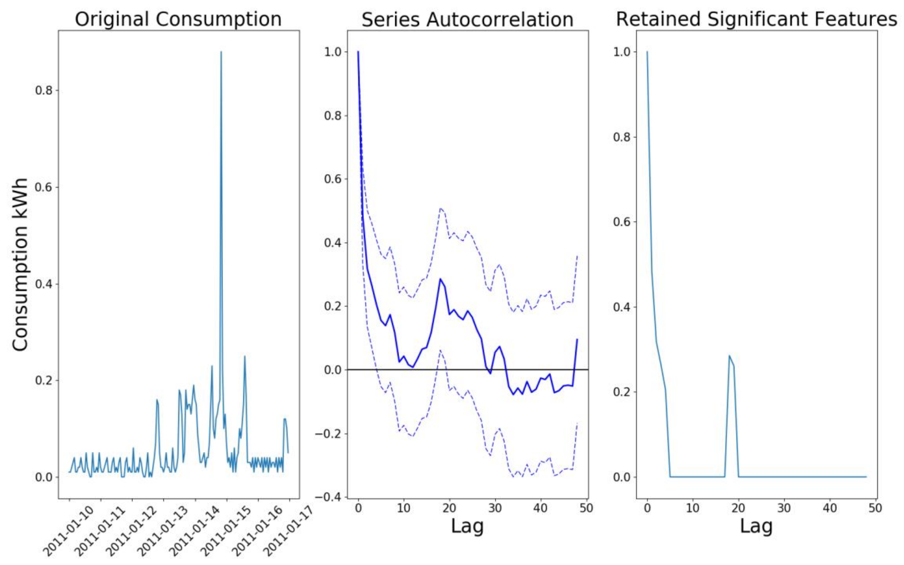
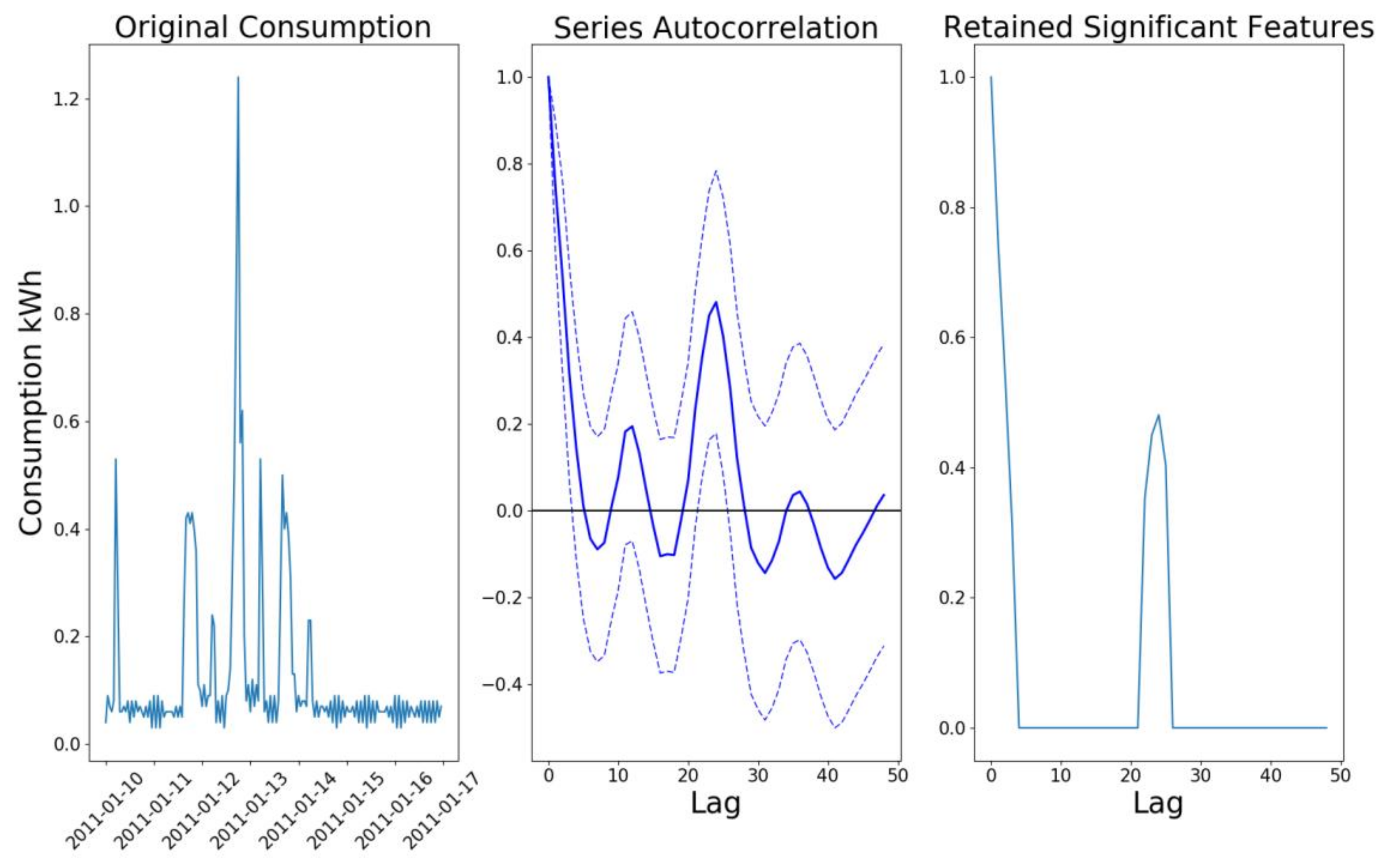
In time series analysis autocorrelation is an essential concept, encompassing the temporal component of the data, e.g., the time dependency in a data series. Autocorrelation is, like correlation, a standardized version of covariance, and is calculated like correlation but as a function of time steps. It quantifies the relation between time steps, called lags. Plotting the autocorrelation coefficients as a function of lag reveals important structures of the data such as trends, seasonality and the stability of the time series [33]. Figure 4, Figure 5 and Figure 6 show different consumption recordings, illustrating different consumption patterns and different autocorrelation functions, with 48 lags. The left side shows the original consumption, while the middle shows the autocorrelation coefficient (solid line) and the 95% confidence interval (dashed line). The right side of the figures shows the significant autocorrelation coefficients. The figures illustrate differences in autocorrelation structures. In Figure 4 the lags indicate no daily cycle and only immediate lags are significant. Figure 5 and Figure 6 exhibit a periodicity in the autocorrelation near lag 20, indicating a recurrent pattern for both consumers.
4.5. Wavelet Feature Extraction
The wavelet transformation is a basis transformation using wavelet basis functions; wavelets can represent smooth and locally non-smooth functions. Wavelets have time and frequency localization, effectively linking time and frequency in contrast to the Fourier transformation which only allows frequency localization [29]. Wavelets are especially well suited for analyzing high frequency data because of their ability to capture global smoothness and local spikes in the signal [34], while filtering out high frequency noise [35]. The application of wavelets for time series feature extraction in this study was inspired by [36]. In the process of filtering high frequency data, wavelets perform efficient data compression by removing non-significant coefficients. Often this process removes a considerable number of coefficients. The decomposition of the signal into wavelet coefficients is not easily interpretable by humans but are readily applicable as input for the K-Means algorithm. The wavelet coefficients are uncorrelated [37].
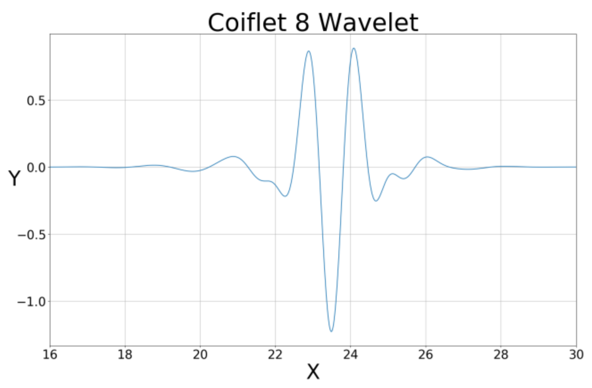
Choosing a suitable wavelet is difficult, as the scaled basis wavelet must be able to encompass the structure of the original signal. We applied the Coiflet 8 wavelet seen in Figure 7, which is highly fluctuating, enabling the encapsulation of high frequency data. We removed non-significant coefficients by applying universal thresholding [38] to the wavelet coefficients. The Python wavelet package PyWt [39] was utilized for the wavelet analysis performed in this paper.
5. Results
This section will describe the results obtained by applying the methodology introduced in Section 4 to the dataset described in Section 3. Section 5.1 will describe clustering with normalized data, while Section 5.2 describes the application of the wavelet transformation and Section 5.3 describes the influence of the autocorrelation feature extraction on the clustering performance. Finally, Section 5.4 will summarize the performed clustering solutions.
5.1. Cluster Permance: Normalized Data
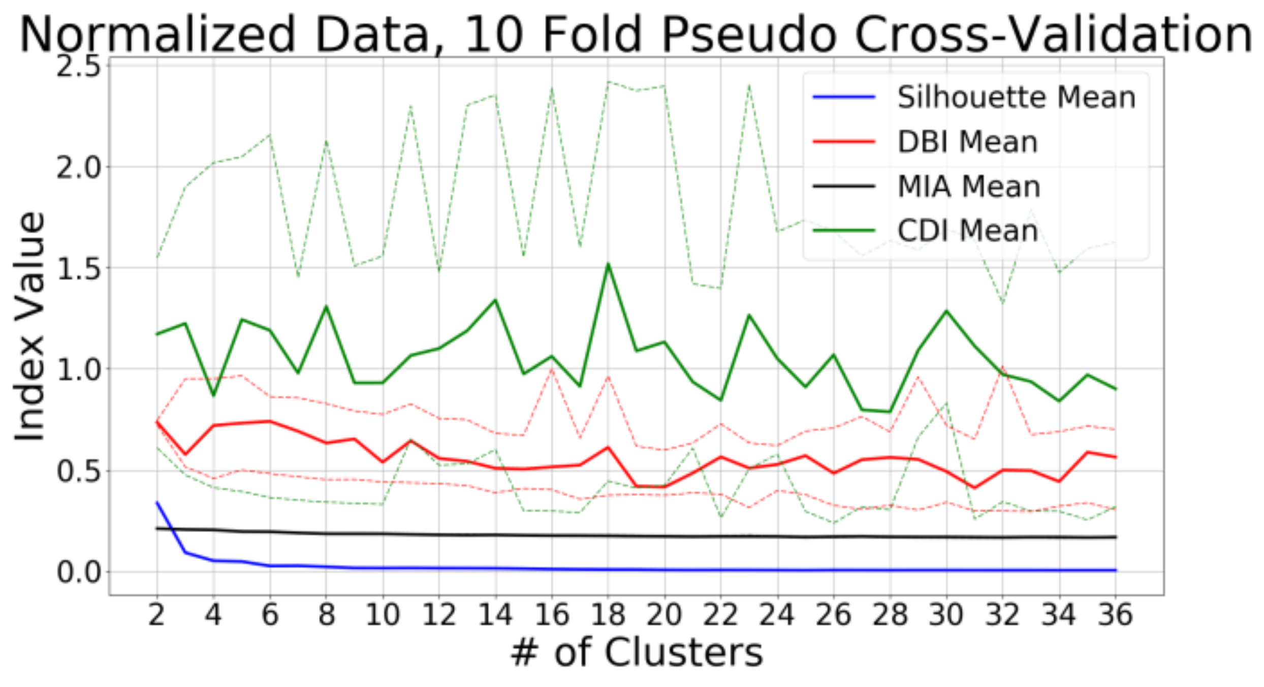
In [19] and various other papers, clustering smart meter consumption by only normalizing data has produced acceptable clustering performance. Clustering the SydEnergi data by only normalizing the data produced the inconclusive cluster validation index graphs seen in Figure 8, indicating a lack of identifiable clusters. Figure 8 shows how the cluster validation indices develop as function of the number of clusters. The dashed lines surrounding the individual indices indicate the maximum and minimum observed values at each selection of clusters calculated by pseudo cross-validation, as described in Section 4.3.5.
As described in Section 4.3, we were looking for an elbow break in the index development, indicating that more clusters will not improve the clustering. The silhouette and MIA indices exhibited very small changes, indicating stability, and both flattened almost immediately, as they were questionable with regards to their performance on the SydEnergi data. Arguably, the silhouette index indicates three clusters, but the structure was poorly defined in the graph and hence we discarded it as a possible optimum number of clusters. The inability of the K-Means to cluster the normalized data can in this case be attributed to the close resemblance of the households included in the study. We included only houses and apartments from the city of Esbjerg connected to district heating.
Normalizing the SydEnergi input data prior to the K-Means clusters, the households included in this analysis were similar in overall grouping, but for 32,000+ consumers the method was expected to reveal sub-clusters. This is an indication that normalization of smart meter data in this case was so subtle that K-Means was unable to identify clusters.
5.2. Cluster Performance: Wavelet Transformation
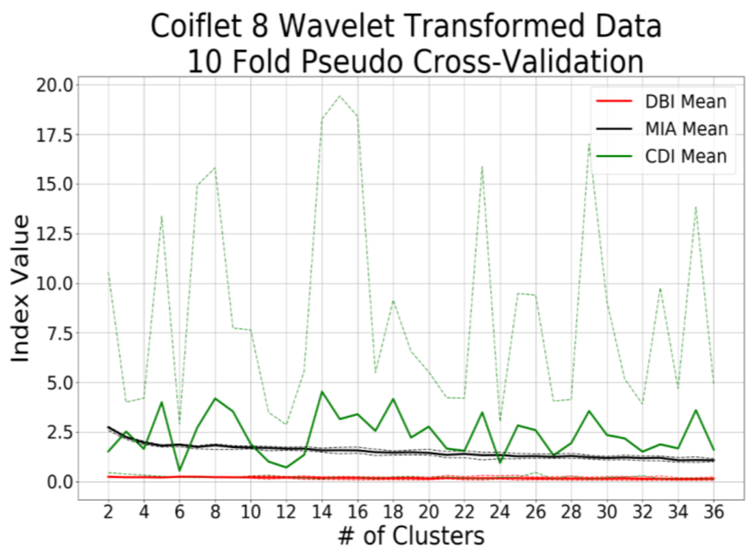
The application of the wavelet transformation of input data resolves the autocorrelation, as the coefficients are uncorrelated. In effect, wavelet transformation performs dimension reduction, keeping the structure of the time series with a reduced number of coefficients. This makes the feature space very similar to the original space, thus—as seen in Figure 9—creating very similar cluster validation indices. In this case, the wavelets did not create more insightful index development and no apparent optimum number of clusters was identifiable. As the wavelet transform compressed the data, the inability to identify clusters was no surprise, as the compressed data was similar to the normalized data. The Python wavelet package; PyWt [39] was unable to calculate the silhouette due to memory overflow issues, attributable to the large data set, and this is thus not included.
5.3. Cluster Performance: Autocorrelation Feature Extraction
The autocorrelation feature extraction (ACF) method—described in Section 4.4—was applied to the data with 24 lags, equivalent to 24 h temporal information. Only statistically significant lags were retained as input data to the K-Means. The transformation reduced the data set size from 32,241 smart meters X 168 hours to 32,241 smart meters X 24 lags (hours). This is a clear reduction of the dataset, with a tangible effect on the computational cost of the K-Means clustering.
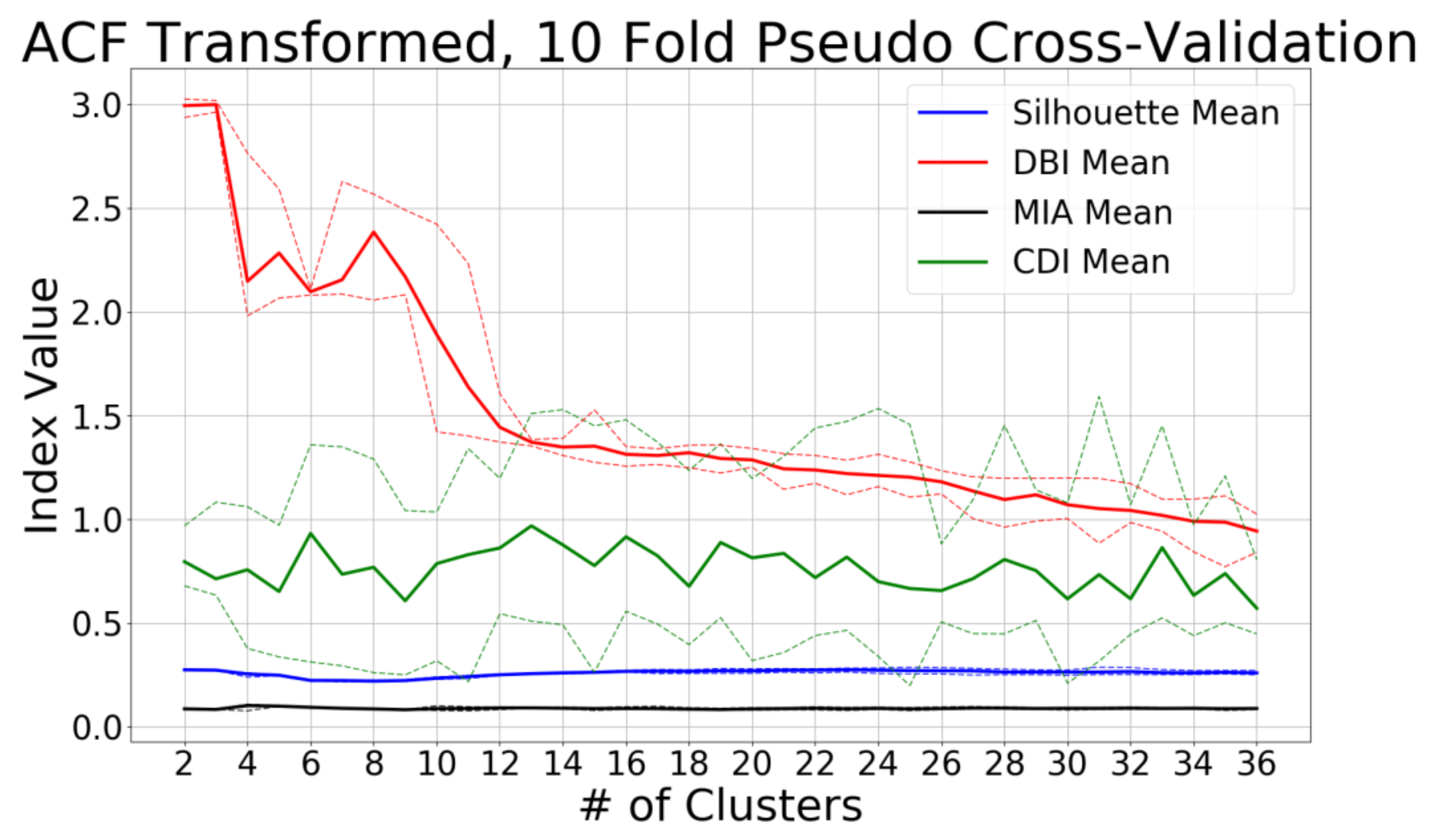
As with the normalized clustering, we calculated the cluster validation index for each number of clusters from 2 to 36; Figure 10 shows the index development. The solid line represents the average index value, with the corresponding dashed lines indicating the maximum and minimum observed values for any given cluster number. In Figure 10, the DBI index shows an “elbow break” at 12 clusters, combined with narrow minimum and maximum bands, implying that 12 clusters is optimum. The MIA and silhouette indices are almost horizontal throughout the entire span of clusters, with very small variation, giving no indication of cluster selection. In contrast, the CDI index exhibits large variation and a jagged horizontal development, also indicating no specific number of clusters. This indicates that the autocorrelation features are potent for the identification of subtle differences in a perceived homogeneous group, enabling even finer clustering.
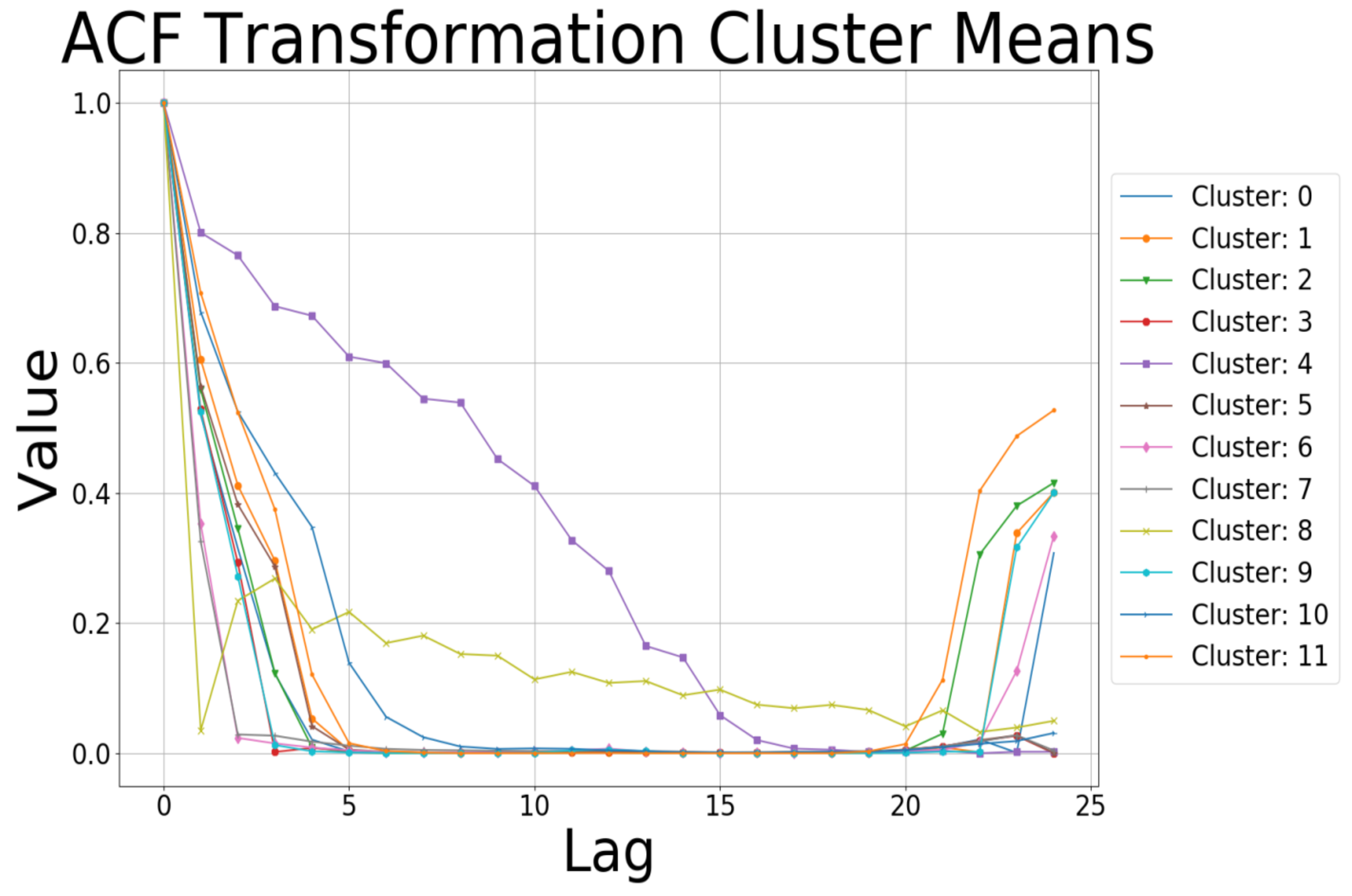
The corresponding plot of the different cluster means in the 12-cluster case is shown in Figure 11. Many of the clusters exhibit similar auto-correlation structures with slight variations in the value and lag offset. Generally, except for clusters 4 and 8, there is a short-term dependency of the past five lags (hours) with zero significant lags in the interval from 5 to 20 lags (hours), and then an indication of recurrent structure. Clusters 4 and 8 are distinctively different from all other clusters; cluster 4 shows a close to linear declining lag function, but no recurrent component, indicating no daily cycle in the consumption pattern. Cluster 8 also exhibits a close to linear decline throughout the 24 lags—except for some fluctuation in the very first lag—and no indication of a 24 hour trend. The remaining clusters have significant lags for the first and final five lags, with different offsets around lag 20 indicating a recurrent consumption pattern. The 12 clusters indicate similar consumption but with slight differences, these differences are attributable to diversity in consumption; although the overall consumption is similar, the finer details are amplified using the autocorrelation features.
The cluster composition of the 12 identified clusters gives further indication of the clustering performance. Table 3 presents an overview of each cluster’s composition in terms of size, dwelling type distribution and postal code distribution. The clusters are well balanced, each accounting for approximately 10% of the total data. In each cluster there is a 40–60% penetration of apartments, indicating, as stated in Section 3, that electricity consumption is influenced more by inhabitants than by dwelling type; apartment or house. Finally, the distribution across postal codes is even according to the size of each postal code. This indicates overall balanced clusters and not just a clustering of select outliers, demonstrating no geographical clustering.
5.4. Comparison of Results
The three different preprocessing methods of the K-Means input data yield very different results. In the data from Esbjerg, where the two household composition groups chosen are very similar, the normalization and the normalization + wavelet transformation were unable to provide any meaningful clustering solution for the data. There was no significant difference in the data structure between normalizing and wavelet transformation of the SydEnergi data. The wavelets do compress and remove autocorrelation, but do not provide the K-Means with the possibility to leverage the autocorrelation. For data where the normalization produced viable clustering solutions, the wavelet transformation was expected to do the same, but with a reduced number of dimensions and thus a significant reduction in computational effort.
With the SydEnergi data, the autocorrelation feature (ACF) method provided clustering solutions that leveraged the autocorrelation inherent in the data. This produced balanced clusters that encompassed the underlying structure found in the consumption patterns of the individual smart meters. The clustering solution generated by ACF was different from the normalization and wavelet transformation solution in that it provided more clusters, but also a different number of clusters. This difference was also observed in [19].
A measure for evaluating the clustering is analyzing the computational effort needed to perform the clustering. All three cases preprocessed the input data. The processes can be run in constant time and their influence on the overall runtime is negligible compared to K-Means lower bound runtime of [40] and upper bound of O(kn) [40], where k is clusters and n is observations. The reduction of the input data via the autocorrelation features or wavelet transformation can result in a significant decrease in the minimum and worst case computational effort needed to cluster the data [19], see Table 4.
6. Discussion
The K-Means clustering algorithm is a simple, efficient and robust method for unsupervised clustering. It is readily implemented in many software suites and easy to apply to numeric data sets. However, the straightforward application of modern data mining software exposes possible pitfalls in data analysis. As this paper shows, it is not possible to calculate meaningful clusters from the SydEnergi data applying the K-Means method directly. Only through careful preprocessing of the input data to enable K-Means to account for temporal components did we calculate meaningful clusters. This demonstrates the importance of understanding and recognizing the data type under analysis. Failing to regard smart meter data as data evolving over time impairs the analysis by not encompassing all available information. Intrinsic data information is not generally utilized in smart meter analysis; reference [4] showed that data type knowledge was not consistently applied in the literature. In the case of smart meter data, the missing information is the autocorrelation, which quantifies how past observations influence current observations.
As described in Section 4.2, K-Means is unable to include autocorrelation, and in effect ignores this intrinsic information. In a supervised—e.g. regression—setting, this could potentially result in singularities, making the problem unsolvable, or at least rendering the coefficients unstable. K-Means robustness ignores this and creates a clustering regardless, not requiring the analyst to reflect upon model and data decisions. This paper has improved on the clustering performance of K-Means by enabling the algorithm to account for intrinsic information. This has been achieved through transformation and feature extraction based on data insights. The preprocessing of the input data enables K-Means to cluster data structures it was not originally intended to include. K-Means input preprocessing was successfully applied in this paper, but also to district heating data [19], where it was applied to reduce within-cluster variance.
K-Means is useful for prototyping, with extensive applications in smart meter clustering. However, the within-cluster variability is consistently large, such that the clusters overlap, delivering academically viable clusters with inconsequential practical value. The overlap results in indistinguishable clusters. There exists a gap in the literature on time series comparison, not just regarding clustering, but also the subsequent evaluation of the similarity of the time series. There exists some literature where various features are extracted from the individual time series and compared. This is a computationally expensive process, which is not always easily automatable. In general, the features proposed and traditional time series analysis have not yet been combined into a strong framework for comparing time series data. Ultimately there is a need for future research into statistically sound methods for evaluating the differences between time series, enabling researchers to better evaluate the resulting clusters and conclude on their (dis)similarity. Without better tools to evaluate differences in time series and reduce the within-cluster variability, smart meter consumption clustering could potentially linger as an academic exercise. This applies not only to smart meter data, but to time series clustering in general.
Not all transformations improve the clustering performance of K-Means. The paper applied several, with only successful application of autocorrelation features. Further, we conducted a principal component analysis with an ensuing substantial reduction in dimensions, however the subsequent clustering of the transformed data showed no improvement compared to the normalization of the input data.
Wavelet transformation was applied and retained much of the general structure of the data in compressed form; thus the cluster validation index development closely resembled the development of the normalized data. The wavelet transformation removed autocorrelation and compressed the data by large factors, resulting in faster performance of the clustering, but with a similar result as that for the original uncompressed data.
The feature extraction methods applied in this paper also reduced the dimensionality of the input data set. This reduction had a significant impact on the computational cost of clustering smart meter data. The wavelet method compresses but maintains the original structure, enabling faster but similar clusters than normalized clustering, while the autocorrelation clusters around data features from the time series and produces different and—for the SydEnergi data—finer-grained clusters.
Mathematics provides a myriad of methods for data manipulation, which can help draw out intrinsic information from data. It requires that the analyst bring knowledge of the data and reflect upon the methods applicable, beyond the popular choices, and that they apply their knowledge to improve the model performance. This paper has shown that careful preprocessing of the data before clustering can improve the clustering performance in several ways, namely speed, the information included in clustering and better cluster definitions by measure of variance.
7. Conclusions
This paper has shown the existence of autocorrelation in specific smart meter electricity data. It is not a general proof of the existence of autocorrelation in all smart meter datasets, but is an indication that smart meter data needs to be examined for autocorrelation before analysis commences. This paper successfully extracted significant autocorrelation coefficients and incorporated them into subsequent clustering using K-Means.
The autocorrelation coefficients, regarded as features, enabled the K-Means algorithms to encompass autocorrelation and deliver more detailed clusters. The resulting clusters are well balanced, with an even distribution of dwelling type within each cluster and across different postal codes. Two clusters were distinctly different from the rest in their overall consumption profile but also in their size, being markedly smaller. In contrast, normalizing the smart meter electricity consumption data was unsuccessful in providing unambiguous clusters. Wavelet transformation of the input data to the K-Means was successful in compressing the data and removing multi-collinearity, but it did not succeed in identifying an optimum number of clusters. Furthermore, this paper implemented an unsupervised version of cross-validation enabling stability measures of the validation indices.
In conclusion, this paper has shown that the clever transformation of data prior to K-Means clustering can improve performance and enable K-Means to handle data and information of types for which it was not originally intended. This result makes it possible to produce clusters from smart meter data that are better defined through smaller clusters with less within-cluster variance.
Acknowledgments
This work is part of the CITIES project funded in part by the Danish Innovation found. Grant DSF 1305-00027B. The data was provided by SydEnergi.
Author Contributions
Alexander Tureczek conceived and designed the study with subsequent analysis. Alexander Tureczek and Per Sieverts Nielsen wrote the paper. Per Sieverts Nielsen and Henrik Madsen reviewed and proofread the paper. Henrik Madsen facilitated the data acquisition for this paper.
Conflicts of Interest
The authors declare no conflict of interest. The founding sponsors had no role in the design of the study; in the collection, analyses, or interpretation of data; in the writing of the manuscript, and in the decision to publish the results.
References
- Dansk Energi (Danish Energy Association). Giv Energien Videre—Nye Energipolitiske Visioner og Udfordringer 2020–2030; Copenhagen, Denmark, 2015; Available online: https://www.danskenergi.dk/udgivelser/nye-energipolitiske-visioner-udfordringer-2020-2030-giv-energien-videre (accessed on 22 February 2018).
- Eurelectric. Vision for the European Electricity Industry; 2018; p. 2. Available online: http://www.eurelectric.org/media/340222/vision_for_the_european_electricity_industry-2017-030-0781-01-e.pdf (accessed on 22 February 2018).
- Chicco, G.; Napoli, R.; Piglione, F.; Postolache, P.; Scutariu, M.; Toader, C. Load pattern-based classification of electricity customers. IEEE Trans. Power Syst. 2004, 19, 1232–1239. [Google Scholar] [CrossRef]
- Tureczek, A.M.; Nielsen, P.S. Structured Literature Review of Electricity Consumption Classification Using Smart Meter Data. Energies 2017, 10, 584. [Google Scholar] [CrossRef]
- Rhodes, J.D.; Cole, W.J.; Upshaw, C.R.; Edgar, T.F.; Webber, M.E. Clustering analysis of residential electricity demand profiles. Appl. Energy 2014, 135, 461–471. [Google Scholar] [CrossRef]
- Park, S.; Ryu, S.; Choi, Y.; Kim, J.; Kim, H. Data-Driven Baseline Estimation of Residential Buildings for Demand Response. Energies 2015, 8, 10239–10259. [Google Scholar] [CrossRef]
- Ozawa, A.; Furusato, R.; Yoshida, Y. Determining the relationship between a household’s lifestyle and its electricity consumption in Japan by analyzing measured electric load profiles. Energy Build. 2016, 119, 200–210. [Google Scholar] [CrossRef]
- Tsekouras, G.J.; Hatziargyriou, N.D.; Member, S.; Dialynas, E.N.; Member, S. Two-Stage Pattern Recognition of Load Curves for Classification of Electricity Customers. IEEE Trans. Power Syst. 2007, 22, 1120–1128. [Google Scholar] [CrossRef]
- Kwac, J.; Flora, J.; Rajagopal, R. Household energy consumption segmentation using hourly data. IEEE Trans. Smart Grid 2014, 5, 420–430. [Google Scholar] [CrossRef]
- Räsänen, T.; Voukantsis, D.; Niska, H.; Karatzas, K.; Kolehmainen, M. Data-based method for creating electricity use load profiles using large amount of customer-specific hourly measured electricity use data. Appl. Energy 2010, 87, 3538–3545. [Google Scholar] [CrossRef]
- Gouveia, J.P.; Seixas, J. Unraveling electricity consumption profiles in households through clusters: Combining smart meters and door-to-door surveys. Energy Build. 2016, 116, 666–676. [Google Scholar] [CrossRef]
- Coke, G.; Tsao, M. Random effects mixture models for clustering electrical load series. J. Time Ser. Anal. 2010, 31, 451–464. [Google Scholar] [CrossRef]
- Granell, R.; Axon, C.J.; Wallom, D.C.H. Impacts of Raw Data Temporal Resolution Using Selected Clustering Methods on Residential Electricity Load Profiles. IEEE Trans. Power Syst. 2015, 30, 3217–3224. [Google Scholar] [CrossRef]
- Chicco, G.; Napoli, R.; Piglione, F. Comparisons Among Clustering Techniques for Electricity Customer Classification. IEEE Trans. Power Syst. 2006, 21, 933–940. [Google Scholar] [CrossRef]
- Chicco, G.; Sumaili Akilimali, J. Renyi entropy-based classification of daily electrical load patterns. IET Gener. Transm. Distrib. 2010, 4, 736–745. [Google Scholar] [CrossRef]
- Mcloughlin, F.; Duffy, A.; Conlon, M. A clustering approach to domestic electricity load profile characterisation using smart metering data. Appl. Energy 2015, 141, 190–199. [Google Scholar] [CrossRef]
- Ndiaye, D.; Gabriel, K. Principal component analysis of the electricity consumption in residential dwellings. Energy Build. 2011, 43, 446–453. [Google Scholar] [CrossRef]
- Kavousian, A.; Rajagopal, R.; Fischer, M. Determinants of residential electricity consumption: Using smart meter data to examine the effect of climate, building characteristics, appliance stock, and occupants’ behavior. Energy 2013, 55, 184–194. [Google Scholar] [CrossRef]
- Tureczek, A. Clustering District Heat Exchange Stations Using Smart Meter Consumption Data. In Proceedings of the 3rd International Conference on Smart Meter Energy Systems and 4th Generation District Heating, Copenhagen, Denmark, 13 August 2017; p. 24. [Google Scholar]
- Billard, L.; Douzal-Chouakria, A.; Samadi, S.Y. An Exploratory Analysis of Multiple Multivariate Time Series. In Proceedings of the 1st International Workshop Advanced Analytics Learning on Temporal Data AALTD 2015, Porto, Portugal, 11 September 2015; Volume 3, pp. 1–8. [Google Scholar]
- Serrà, J.; Arcos, J.L. An empirical evaluation of similarity measures for time series classification. Knowl.-Based Syst. 2014, 67, 305–314. [Google Scholar] [CrossRef]
- Carpaneto, E.; Chicco, G.; Napoli, R.; Scutariu, M. Electricity customer classification using frequency—Domain load pattern data. Int. J. Electr. Power Energy Syst. 2006, 28, 13–20. [Google Scholar] [CrossRef]
- Chicco, G.; Ionel, O.M.; Porumb, R. Electrical load pattern grouping based on centroid model with ant colony clustering. IEEE Trans. Power Syst. 2013, 28, 1706–1715. [Google Scholar] [CrossRef]
- Kang, J.; Lee, J. Electricity Customer Clustering Following Experts’ Principle for Demand Response Applications. Energies 2015, 8, 12242–12265. [Google Scholar] [CrossRef]
- Viegas, J.L.; Vieira, S.M.; Melício, R.; Mendes, V.M.F.; Sousa, J.M.C. Classification of new electricity customers based on surveys and smart metering data Commission for Energy Regulation. Energy 2016, 107, 804–817. [Google Scholar] [CrossRef]
- Ramos, S.; Duarte, J.M.; Duarte, F.J.; Vale, Z. A data-mining-based methodology to support MV electricity customers’ characterization. Energy Build. 2015, 91, 16–25. [Google Scholar] [CrossRef]
- Liu, X.; Nielsen, P.S. Regression-based Online Anomaly Detection for Smart Grid Data. arXiv, 2016; in press. [Google Scholar]
- Lattin, J.; Carrol, J.D.; Green, P.E. Analyzing Multivariate Data, 1st ed.; Thomson Brooks/Cole: Duxbury, MA, USA, 2004; Volume 46. [Google Scholar]
- Friedman, J.; Hastie, T. The Elements of Statistical Learning, 1st ed.; Springer: Berlin/Heidelberg, Germany, 2008. [Google Scholar]
- Pedregosa, F.; Varoquaux, G.; Gramfort, A.; Michel, V.; Thirion, B.; Grisel, O.; Blondel, M.; Prettenhofer, P.; Weiss, R.; Dubourg, V.; et al. Scikit-learn: Machine Learning in Python. J. Mach. Learn. Res. 2012, 12, 2825–2830. [Google Scholar]
- Al-otaibi, R.; Jin, N.; Wilcox, T.; Flach, P. Feature Construction and Calibration for Clustering Daily Load Curves from Smart-Meter Data. IEEE Trans. Ind. Inform. 2016, 12, 645–654. [Google Scholar] [CrossRef]
- Perry, P.O. Cross-Validation for Unsupervised Learning. arXiv, 2009; in press. [Google Scholar]
- Madsen, H. Time Series Analysis; Chapman & Hall/CRC: Boca Raton, FL, USA, 2008. [Google Scholar]
- Wasserman, L. All of Statistics; Springer: Berlin/Heidelberg, Germany, 2003; Volume C. [Google Scholar]
- Barford, L.A.; Fazzio, R.S.; Smith, D.R. An Introduction to Wavelets; Technical Report HPL-92-124; Hewlett-Packard Labs: Bristol, UK, 1992; Volume 2, pp. 1–29. [Google Scholar]
- Morchen, F. Time Series Feature Extraction for Data Mining Using DWT and DFT; 2003; pp. 1–31. Available online: http://www.mybytes.de/papers/moerchen03time.pdf (accessed on 22 February 2018).
- Li, T.; Li, Q.; Zhu, S.; Ogihara, M. A survey on wavelet applications in data mining. ACM SIGKDD Explor. Newsl. 2002, 4, 49–68. [Google Scholar] [CrossRef]
- Wasserman, L. All of Nonparametric Statistics; Springer: New York, NY, USA, 2006. [Google Scholar] [CrossRef]
- Wasilewski, F. PyWavelets; 2006; Available online: https://pywavelets.readthedocs.io/en/latest/ (accessed on 22 February 2018).
- Arthur, D.; Vassilvitskii, S. How slow is the k-means method? In Proceedings of the Twenty-Second Annual Symposium on Computational Geomeometry, Sedona, AZ, USA, 5–7 June 2006; p. 144. [Google Scholar]
Figure 1.
Four different meters all exhibiting a week-on-week consumption increase above 200%. This is to filter out dwellings that were vacant during the week analyzed, as we were not interested in clustering standby consumption.
Figure 1.
Four different meters all exhibiting a week-on-week consumption increase above 200%. This is to filter out dwellings that were vacant during the week analyzed, as we were not interested in clustering standby consumption.

Figure 2.
Methodology flow chart. This chart illustrates the different data processing methods applied. The (blue) boxes indicate processes to which all methods were applied, namely data, preparation and clustering. After preparation, autocorrelation (red) indicates the extraction of autocorrelation features. Normalization (black) was applied both as a sole processing method, but also in preparation for wavelet transformation (green).

Figure 3.
(Left): A scatter of points collapsed to have no temporal component. The three colors indicate three different clusters, but it is not possible to identify overlap. (Right): The scatter has been expanded by its original temporal component.
Figure 3.
(Left): A scatter of points collapsed to have no temporal component. The three colors indicate three different clusters, but it is not possible to identify overlap. (Right): The scatter has been expanded by its original temporal component.

Figure 4.
(Left) The original consumption profile, (Middle) the solid line is the autocorrelation coefficient, dashed lines are the 95% confidence intervals. (Right) Significant autocorrelation coefficients retained as meter features and applied as input to K-Means clustering. The significant lags only include the first 14 lags, indicating no recurrent pattern.

Figure 5.
(Left) The original consumption profile, (Middle) the solid line is the autocorrelation coefficient, dashed lines are the 95% confidence intervals. (Right) Significant autocorrelation coefficients retained as meter features and applied as input to K-Means clustering. The significant lags include lags from the first five lags and a recurrence at around lag 20, indicating some periodicity in the consumption.

Figure 6.
(Left) The original consumption profile, (Middle) the solid line is the autocorrelation coefficient, dashed lines are the 95% confidence intervals. (Right) Significant autocorrelation coefficients retained as meter features and applied as input to K-Means clustering. The significant lags include lags from the first five lags and a recurrence at around lag 20, indicating some periodicity in the consumption. The significant lags are distinct from the lags in Figure 5.

Figure 7.
The Coiflet 8 wavelet applied in this paper. It exhibits a similar structure to the meter data, making it a suitable candidate for the wavelet transformation of the input data.
Figure 7.
The Coiflet 8 wavelet applied in this paper. It exhibits a similar structure to the meter data, making it a suitable candidate for the wavelet transformation of the input data.

Figure 8.
Cluster validation indicator development as a function of clusters. The silhouette and MIA validation indices were non-informative in this data set. While the CDI index exhibits large variation, there is no indication of optimum cluster selection, which was also the case for the DBI index.

Figure 9.
Cluster validation index development from 2 to 36 clusters using Coiflet 8 wavelet transformation. Significance was established applying universal thresholding. No apparent structure was found in the development of the three indices. As with normalized data, the CDI exhibited large fluctuations, while MIA and DBI had very controlled fluctuations.

Figure 10.
Cluster validation index development for the autocorrelation features (ACF). The DBI index shows a distinct “elbow” break at 12 clusters.
Figure 10.
Cluster validation index development for the autocorrelation features (ACF). The DBI index shows a distinct “elbow” break at 12 clusters.

Figure 11.
Plot of the 12 autocorrelation function cluster means (ACF) identified using the CDI. Clusters 4 and 8 are distinctly different showing linear decline and no recurrence. The remaining clusters exhibit a largely similar structure, with different values, and a different lag for recurrence.
Figure 11.
Plot of the 12 autocorrelation function cluster means (ACF) identified using the CDI. Clusters 4 and 8 are distinctly different showing linear decline and no recurrence. The remaining clusters exhibit a largely similar structure, with different values, and a different lag for recurrence.


Table 1.
Initial data description of SydEnergi data for the city of Esbjerg, comprising 13 distinct quantitative measures of the data applied in the paper. As introduced in [4].
Table 1.
Initial data description of SydEnergi data for the city of Esbjerg, comprising 13 distinct quantitative measures of the data applied in the paper. As introduced in [4].
| Data Description | Value |
|---|---|
| Country | Denmark |
| Region | Region Syd (Region South) postal codes: 6700, 6705, 6710, 6715 (City of Esbjerg) |
| Supplier | SydEnergi Electricity Utility |
| Initial Size | 34,418 m |
| Clear Reduction | Confer Table 2. |
| Missing Values | 70 m |
| Final Size | 32,241 |
| Recording Frequency | 60 min |
| Start | 10 January 2011 |
| End | 16 January 2011 |
| Length | 168 observations (hourly readings) |
| Type | Single family house (18,058 initial size) Apartments (15,721 initial size) both heated via district heating. |
| Referral | Data has never before been referenced. |
Table 2.
Data cleaning waterfall. Filter indicates the removal criteria and Meters show the remaining meters after the application of the filter. Discard is the number of meters discarded through the filtering. Final bulk is the number of meters ready for analysis after the cleaning of data.
Table 2.
Data cleaning waterfall. Filter indicates the removal criteria and Meters show the remaining meters after the application of the filter. Discard is the number of meters discarded through the filtering. Final bulk is the number of meters ready for analysis after the cleaning of data.
| Filter | Meters | Discard | Note |
|---|---|---|---|
| Initial Data | 34,418 | - | Original data |
| Missing | 34,348 | 70 | Removal of meters with missing recordings |
| Mean Zero | 33,325 | 1023 | Removal of meters with 0 mean indicating no consumption |
| Median Zero | 32,745 | 580 | Removal of meters with 0 median indicating no consumption |
| Variance Zero | 32,745 | 0 | Removal of meters with 0 variance indicating flat consumption |
| Consumption < 0 | 32,744 | 1 | Removal of meters with <0 consumption indicating prosumers |
| Overlapping | 32,586 | 158 | Overlapping with 2nd week for comparison |
| +200% Increase | 32,241 | 345 | +200% consumption increase from (10th–16th) to (17th–23rd) |
| Final bulk | 32,241 | - | Final number of meters included in analysis |
Table 3.
Cluster composition table of the 12 different clusters. Only clusters 4 and 8 are markedly different from rest, with a very small cluster size. The remaining clusters sizes are well-balanced across all parameters.
Table 3.
Cluster composition table of the 12 different clusters. Only clusters 4 and 8 are markedly different from rest, with a very small cluster size. The remaining clusters sizes are well-balanced across all parameters.
| Cluster Composition | Dwelling Type | Postal Code in Esbjerg | ||||||
|---|---|---|---|---|---|---|---|---|
| Cluster | Size | % of Total Data | Apartments | Houses | 6700 | 6705 | 6710 | 6715 |
| 0 | 3198 | 9.92% | 1244 | 1954 | 1396 | 571 | 754 | 477 |
| 1 | 2456 | 7.62% | 851 | 1605 | 976 | 460 | 609 | 411 |
| 2 | 3342 | 10.37% | 1240 | 2102 | 1427 | 603 | 798 | 514 |
| 3 | 3988 | 12.37% | 1920 | 2068 | 1953 | 739 | 763 | 533 |
| 4 | 239 | 0.74% | 117 | 122 | 127 | 36 | 45 | 31 |
| 5 | 4295 | 13.32% | 1854 | 2441 | 1956 | 846 | 888 | 605 |
| 6 | 3014 | 9.35% | 1616 | 1398 | 1522 | 586 | 489 | 417 |
| 7 | 3590 | 11.13% | 2237 | 1353 | 1976 | 674 | 539 | 401 |
| 8 | 405 | 1.26% | 300 | 105 | 256 | 63 | 46 | 40 |
| 9 | 3703 | 11.48% | 1476 | 2227 | 1568 | 670 | 868 | 597 |
| 10 | 1794 | 5.56% | 859 | 935 | 875 | 344 | 347 | 228 |
| 11 | 2217 | 6.88% | 946 | 1271 | 940 | 462 | 488 | 327 |
| Total | 32,241 | 100.00% | 14,660 | 17,581 | 14,972 | 6054 | 6634 | 4581 |
Table 4.
Clustering method runtime comparison. The normalized and wavelet methods were unable to provide meaningful clusters and are for comparison set to 12 clusters and 25% compression for wavelets. The autocorrelation and wavelet method reduced the dataset size, with a significant impact on the runtime. The table is an adaptation from a table in [19].
| Processing | Normalization | Autocorrelation Features | Wavelet |
|---|---|---|---|
| Scaling/Transform | Constant time | Constant time | Constant time |
| Size of input data (n) | 168 × 32k+ | 24 × 32k+ | 42 × 32k+ |
| Best case running time (12 clusters) | |||
| Worst case running time (12 clusters) | 12168 | 1224 | 1242 |
© 2018 by the authors. Licensee MDPI, Basel, Switzerland. This article is an open access article distributed under the terms and conditions of the Creative Commons Attribution (CC BY) license (http://creativecommons.org/licenses/by/4.0/).
Share and Cite
MDPI and ACS Style
Tureczek, A.; Nielsen, P.S.; Madsen, H. Electricity Consumption Clustering Using Smart Meter Data. Energies 2018, 11, 859. https://doi.org/10.3390/en11040859
AMA Style
Tureczek A, Nielsen PS, Madsen H. Electricity Consumption Clustering Using Smart Meter Data. Energies. 2018; 11(4):859. https://doi.org/10.3390/en11040859
Chicago/Turabian StyleTureczek, Alexander, Per Sieverts Nielsen, and Henrik Madsen. 2018. "Electricity Consumption Clustering Using Smart Meter Data" Energies 11, no. 4: 859. https://doi.org/10.3390/en11040859
Note that from the first issue of 2016, this journal uses article numbers instead of page numbers. See further details here.