A General Approach to Enhance Short Wave Satellite Imagery by Removing Background Atmospheric Effects

Swedish Meteorological and Hydrological Institute (SMHI), SE-60176 Norrköping, Sweden
*
Author to whom correspondence should be addressed.
Remote Sens. 2018, 10(4), 560; https://doi.org/10.3390/rs10040560
Submission received: 2 February 2018
/
Revised: 23 March 2018
/
Accepted: 26 March 2018
/
Published: 5 April 2018
(This article belongs to the Special Issue Atmospheric Correction of Remote Sensing Data)
Abstract
:Atmospheric interaction distorts the surface signal received by a space-borne instrument. Images derived from visible channels appear often too bright and with reduced contrast. This hampers the use of RGB imagery otherwise useful in ocean color applications and in forecasting or operational disaster monitoring, for example forest fires. In order to correct for the dominant source of atmospheric noise, a simple, fast and flexible algorithm has been developed. The algorithm is implemented in Python and freely available in PySpectral which is part of the PyTroll family of open source packages, allowing easy access to powerful real-time image-processing tools. Pre-calculated look-up tables of top of atmosphere reflectance are derived by off-line calculations with RTM DISORT as part of the LibRadtran package. The approach is independent of platform and sensor bands, and allows it to be applied to any band in the visible spectral range. Due to the use of standard atmospheric profiles and standard aerosol loads, it is possible just to reduce the background disturbance. Thus signals from excess aerosols become more discernible. Examples of uncorrected and corrected satellite images demonstrate that this flexible real-time algorithm is a useful tool for atmospheric correction.
1. Introduction
Any satellite based Earth remote sensing application has to deal with the atmosphere. Either the atmosphere (and its constituents) itself is in the focus of the study or it is regarded as a source of perturbation. The latter applies when the scope is observation of phenomena on the surface of the Earth. For instance in ocean color applications when the purpose is the retrieval of information on substances and particles in the water, the atmosphere is obscuring the upwelling radiance observed by the satellite. Interactions of sunlight and atmospheric particles can lead to a reduced reflection (absorption by gases or aerosols above bright surface), increased reflection (Rayleigh scattering by molecules or Mie scattering by aerosols above dark surface) or may even result in a net horizontal transport (in case of horizontal inhomogeneity). As the atmospheric path length varies with scanning angle, the atmospheric effects on the signal at interest may vary strongly, depending on the spectral range, all within one satellite scene. Thus, in order to retrieve consistent information on atmospheric phenomena, it may require properly describing this scan-dependent impact on the observation.
Man made or natural, phenomena with large environmental impact such as smoke from forest fires and desert dust can be observed by satellites passively measuring radiance in the visible part of the spectral range. However, in order for those phenomena to be easily discernible in satellite imagery the effects of the atmospheric background due to water vapor, Ozone, other gaseous constituents, and background aerosols, need to be accounted for. The problem is well understood and tools are at hand to solve the radiative transfer equation numerically to an adequate precision (e.g., [1] or [2]). However, in addition to the comprehensive computational efforts, a thorough solution also requires extensive auxiliary information, such as aerosol loads, water vapor content, Ozone content, and surface characterization.
Newer satellite imaging instruments have the capability to derive aerosol optical properties. However, still, the approach, accuracy and type of product depend strongly on the available channels and their spectral response functions. Algorithms, based on more or less independent data (i.e., data from other sources than the imager itself) would therefore be hard to adapt to other instruments. In contrast, the dependence on other data than the satellite observations makes it challenging for operational applications, not just because of the required timeliness, but also due to the reliability of such data: A Numerical Weather Prediction (NWP) model may provide fairly accurate estimations of Ozone content and water vapor, however, the latter is more sensitive to synoptic and sub-synoptic scale weather patterns and therefore more prone to inaccurate modeling. Further, it is not possible in todays forecast models to get the actual atmospheric aerosol load accurately enough to be applied in satellite retrievals supposed to work on the km-scale.
Many existing algorithms address the problem of atmospheric interference on surface reflection. The Simplified Method for Atmospheric Correction (SMAC) [3] and the model of Sandmeier and Itten [4] use plane-parallel radiative transfer models, which, for large viewing zenith angle (as for full-disk geostationary imagery) or at low sun elevations (most pronounced in polar regions), would lead to large systematic errors. Others, like the MODIS Corrected Reflectance (CREFL) [1] algorithm, support only a limited set of sensors or satellites, and are not easily adaptable. Radiative transfer calculations are still very time consuming, and the many auxiliary data required may easily make the calculations extensive and costly, and thus not possible to apply for real-time operational purposes. Instead radiative transfer calculations need to be run offline to produce faster accessible look-up tables (LUTs), or calculations need to be parameterized. The latter has the disadvantage that every time a new sensor arrives a new calculation of sensor specific parameters needs to be derived. What we will present here is a method where sensor and method are decoupled, so one set of LUTs allows to derive corrections for all imagers operating in the visible spectral range.
The main aim of the approach presented in this paper is to provide an easy to use tool that allows generating high contrast true color imagery by correcting for the most prominent atmospheric effects, i.e., scattering and absorption for both gaseous constituents as well as standard aerosols. The method is valid globally under all sun-satellite viewing conditions and applicable to any satellite sensor with spectral capability in the visible spectral range. Atmosphere corrected true color imagery is an important support to real-time forecasting and monitoring of events like smoke from forest/grass fires and desert dust, potentially affecting areas like aviation and public health. The method is implemented in the open source software package Pyspectral, which is part of the Pytroll suite of free and open source Python packages [5].
Theoretical background of how atmospheric interaction influences satellite observed surface reflection and which approach is chosen to reduce its effect is given in Section 2. The algorithm itself is explained in detail in Section 3. Pyspectral, and examples how it together with other Pytroll packages, can be used to easily generate true color images is introduced in Section 4. Section 5 gives examples of uncorrected and corrected images. It is followed by a short summary and our conclusions in Section 6.
2. Theoretical Background
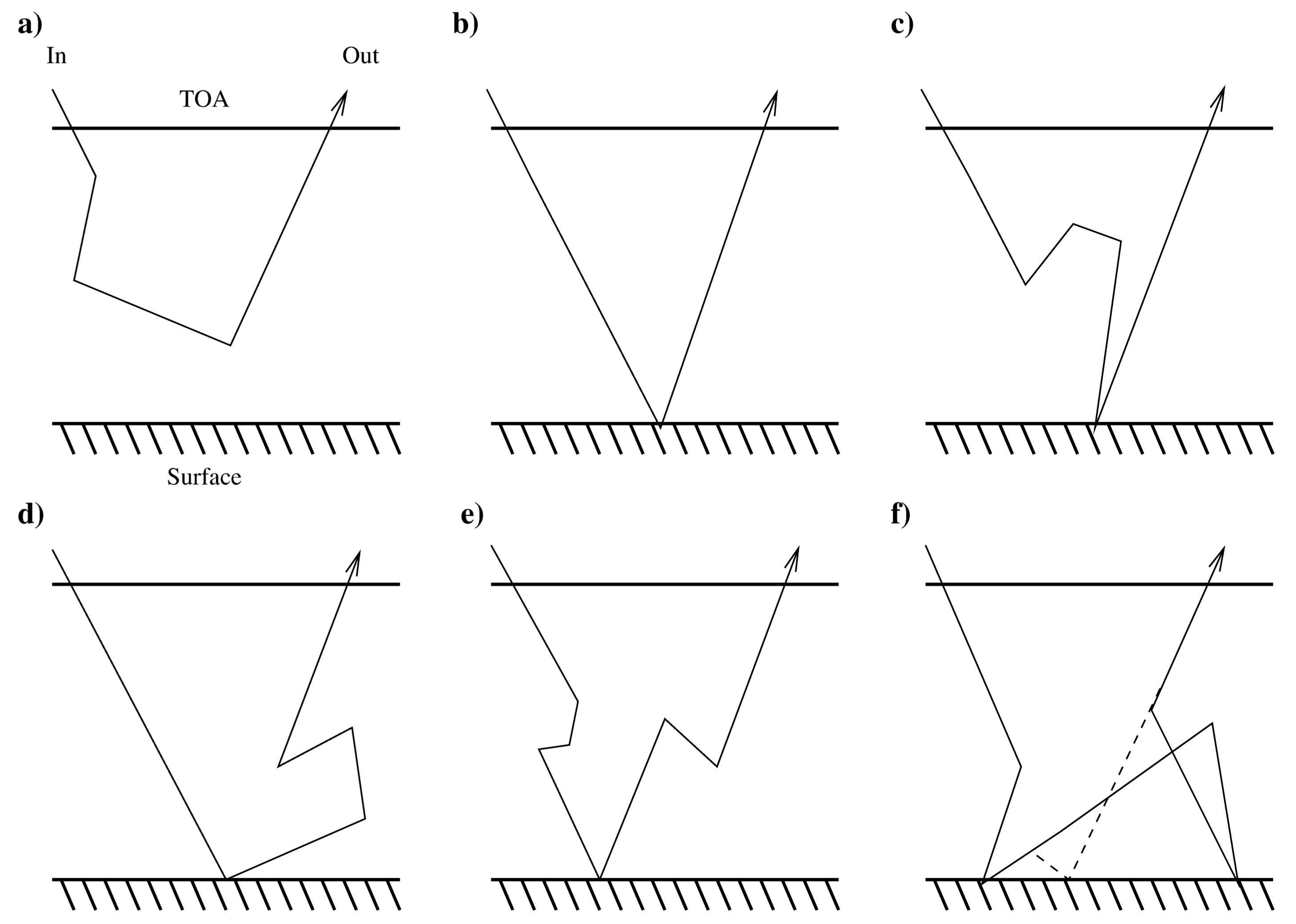
Information transfered from Earth to a space-born instrument via light beams depends strongly on their path and interactions of light and matter. Figure 1 according to [6] shows schematic pathways on how solar light beams (the arrow) may reach the satellite detector. An interaction (scattering) of light and matter is displayed by a change of the arrows direction. Direct information from the surface (which means no further interaction after surface-contact) can be carried by rays of light traveling as shown in sketches b and c and dashed parts of f. Light that does not reach the detector is also part of the signal. When light is scattered out of the beam or absorbed by the surface, it does contribute to the spectral composition of the RGB image by changing the color of the pixel. Light rays which do not touch the ground at all (sketch a) and thus do not carry any information of the surface or overwrite their surface information (sketches d, e and solid parts of f) by interaction with atmospheric particles after the surface reflection are the noise that we want to remove from the image. Sketch f collects all light beams hitting the ground more often than just once. The last interaction before hitting the detector may be of both origins, atmospheric (solid) or surface (dashed). It is sampled together because of its relative low contribution, especially for conditions with low surface reflections (compare Table 1, last column).
A simple study with the 3D Monte Carlo radiative transfer model GRIMALDI [7] is used to identify the most relevant sources of distortion. It allows quantifying the importance of individual paths. The percentage contribution for different solar zenith angle - surface albedo combinations is displayed in Table 1. Note that the residuum goes to atmospheric and surface absorption. In general, Table 1 shows that the numbers increase (except for a, which is completely independent of surface properties) with increasing surface albedo. This is simply because of fewer light beams being taken out of the system by surface absorption. Any individual setting is dominated by a and b. While b increases with increasing surface albedo, a increases with increasing solar zenith angle. Contaminations from rays of light with atmospheric interaction after surface contact (d, e and parts of f) do also increase with increasing surface albedo, however, their contribution remains low compared to light beams carrying the signal (b). So a perfect atmospheric correction algorithm would remove contributions from a, d, e and parts of f because these cases feature light-atmosphere interactions before reaching the detector and thus contaminate the surface signal.
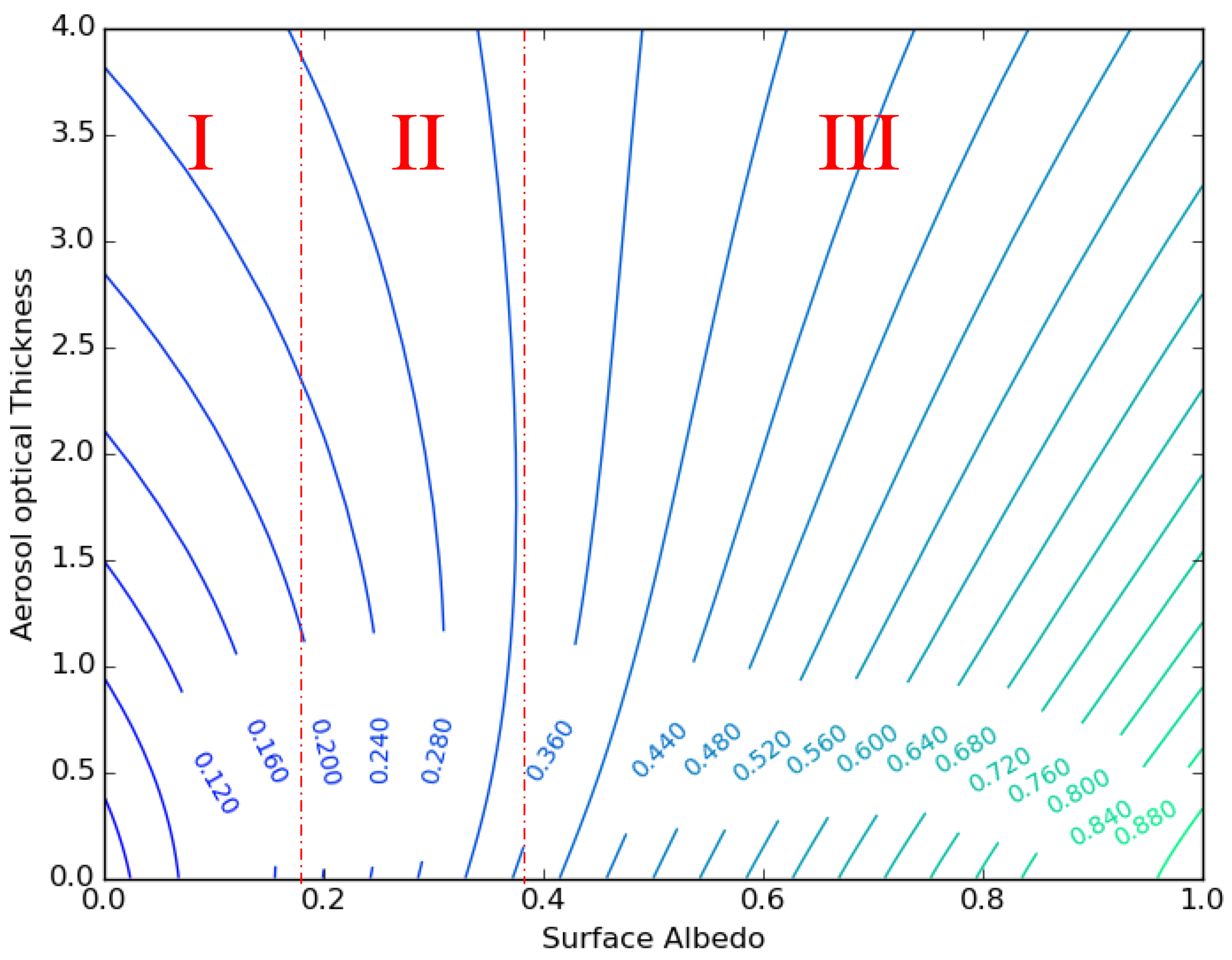
Detailed information of the atmospheric composition (water vapor and aerosol species and distribution, etc.) and extensive in-line radiative transfer calculations or complex sets of look-up tables would be needed for a quantitative correct estimate of the atmospheric noise content. Therefore, this algorithm focuses on the qualitative enhancement of physical RGB image features and not on quantitative feature retrievals. Figure 2 illustrates how complex reflection modifications by aerosols may look.
In-depth knowledge of the atmospheric composition without the use of auxiliary data is impossible for most applications. Auxiliary data, on the other hand hamper flexibility and adaption to new instruments. The other alternative, built-in retrievals of atmospheric properties would require other channels to provide information. Since the information content of satellite channels in accordance to aerosol and gaseous properties depends on the spectral response function of the detector, it would be even more demanding, if not impossible, to adapt such an algorithm to other instruments.
In order to achieve a flexible (i.e., easy to adapt to other/new instruments) algorithm that is sufficiently fast for real-time applications, the strategy we follow in this approach is to remove theoretical contributions from light rays without surface contact, with climatological gaseous and aerosol composition and smooth out the correction for highly reflective targets like for example clouds or snow covered areas.
3. Method
3.1. Radiative Transfer Simulations
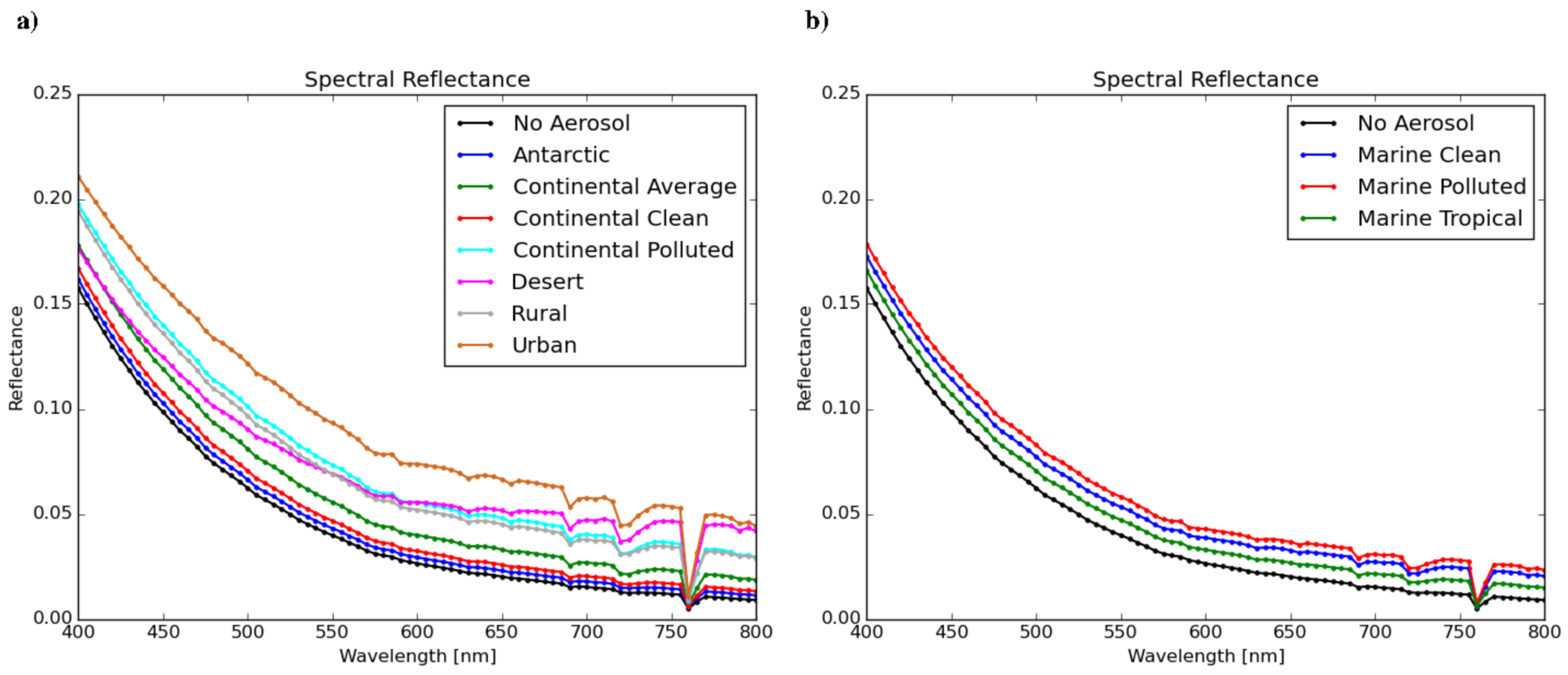
The atmospheric contribution to the observed reflection (i.e., Table 1 a) is estimated by means of radiative transfer calculations. Simulations are performed with a black surface (albedo = 0 to exclude all contributions from the ground), varying observation and sun geometry, and different compositions of standard atmospheres and background aerosols (see Table 2). DISORT [11], a model using the discrete-ordinate-method from the package libRadtran [8] version 2.0 is the selected solver. Atmospheric standard profiles, based on McClatchey’s work [12] are used here. Rayleigh scattering is calculated from particle density, gaseous absorption from profiles of ozone, oxygen, water vapor, carbon dioxide and nitrogene dioxide. Aerosol scattering and absorption is calculated from Mie-theory. Most of the background aerosols are recommended mixtures from the OPAC software package [13] (antarctic, avarage continental, clean continental, polluted continental, desert, clean marine, polluted marine, tropical marine, and urban) and one (rural) is the libRadtran standard aerosol profile [14].
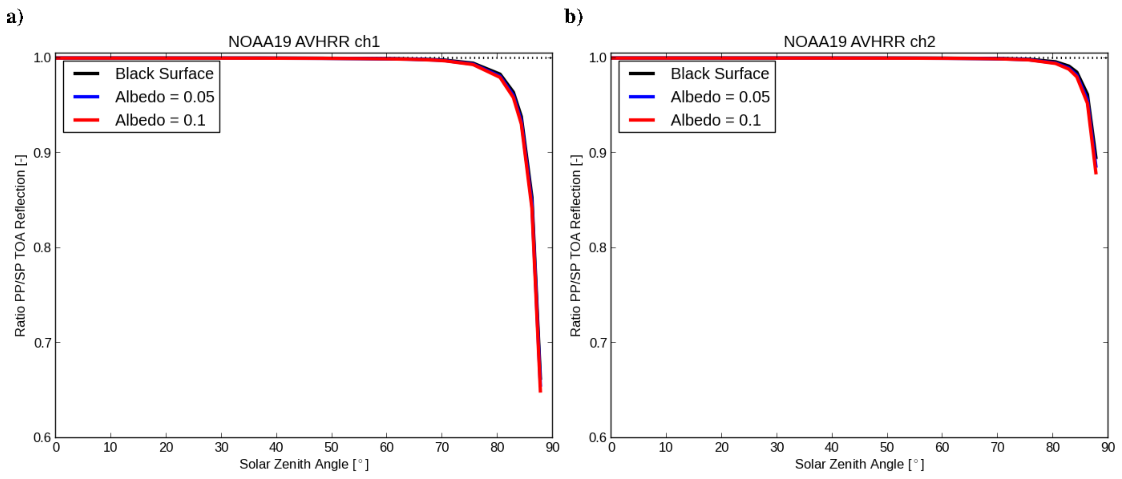
In a previous study [15] it has been shown, that the assumption of a plane-parallel atmosphere may lead to considerable deviations in TOA reflections (see Figure 3). Channels in the solar spectral range (or general low-wavelength-channels) are especially susceptible to errors. To allow for global application (including polar regions) of this algorithm and under all possible illumination conditions, a pseudo-spherical setting was selected for the radiative transfer simulations.
3.2. Look-Up Tables
As outlined in Table 2 the radiative transfer simulations were done in wavelength steps of 5 nm over the entire visible spectral range, and for each atmosphere and aerosol profile varying the three sun-satellite observation angles as detailed. This resulted in around million radiative transfer simulations. From Table 2 we see that the simulations have been done for equidistant zenith angles up to degrees, corresponding to a secant, () equals 3 for both the zenith angles, and further in non-equidistant steps for the solar zenith angles up to a secant of 25, corresponding to a sun elevation of a little more than 2 degrees.
As the path length of the signal is proportional to the satellite and sun secants, rather than the angles, we stored the results in HDF5 files using secant for the Solar and satellite angles. In order to have radiative transfer calculations for all daylight situations we have interpolated the simulations along the axis of the Solar zenith secant above all the way to using steps of . This results in 96 = 3,102,624 (81 wavelengths, 19 azimuth angles, 21 satellite zenith angles and 96 sun-zenith angles) simulations for each atmosphere and aerosol profile, thus more than 200 million reflectance correction values, which we have stored in 66 individual HDF5 files (one for each atmosphere and aerosol profile). These HDF5 files provide Look-Up Tables (LUTs) which can be used in a computer program for fast calculations of the atmosphere corrected reflectance applicable to a given satellite observation.
3.3. Adaptation to Specific Channel
The radiative transfer simulations are monochromatic and strictly applicable only to a narrow band around each wavelength in the 5 nm resolution available in the LUTs. To get a reflectance correction for a given spectral band one should in principle convolve the relative spectral response function with reflectance obtained from simulations with a resolution in wavelength which is much higher than the width of the band. However, in the vast dominant part of the visible spectrum the effects of molecular and aerosol absorption and scattering is very smooth as a function of wavelength. Only towards the higher end of the wavelength spectrum from around 700 nm is this picture slightly distorted (cf. Figure 4).
Since reflectance corrections are available at a resolution comparable to the typical sensor band width (see Figure 5), convolution is not necessary. Instead we derive an effective wavelength and then find the two closest wavelengths in the LUT and make a linear interpolation between the two corrections. The effective wavelength is the average of the wavelength over the response function weighted by . This weighting function takes care of the fact that the Rayleigh scattering is proportional to the reciprocal of the wavelength to the fourth power.
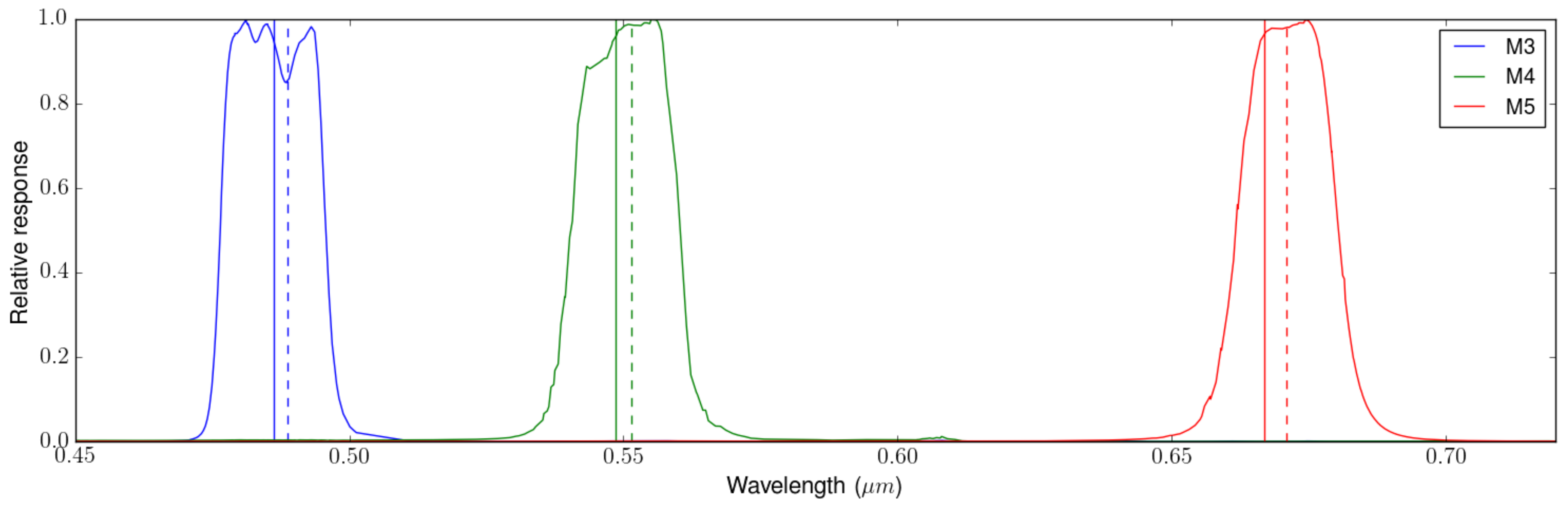
Figure 5 shows spectral responses and the central and effective wavelengths for the three visible M-bands of the VIIRS sensor on board the Suomi-NPP satellite commonly used to generate true color imagery from this sensor.
3.4. Application to Satellite Imagery
The method outlined, using a set of LUTs with the contribution to the TOA reflectance from the atmospheric effects described in sketch a of Figure 1, as a function of wavelength and sun-satellite observation geometry, allows for atmospheric correction of satellite imagery in real-time. Besides the observed visible reflectances the method requires additional ancillary data as input. The effective wavelength is of course mandatory input, and so are for each pixel the satellite view zenith angle, the solar zenith angle, and the satellite-sun azimuth difference angle. In addition a land-sea mask in pixel resolution can be used to perform a land-sea dependent atmospheric correction.
The correction derived from the LUTs applies strictly only to surface targets with a complete cloud free line of sight to the satellite sensor through the entire atmosphere. For elevated or cloud covered targets the atmospheric correction derived from the LUTs would be too strong. To account for this we apply a simple method using the observed reflectance in the red part of the visible spectrum around . High reflectance in the red part of the visible spectrum is an adequate proxy for presence of clouds as well as snow covered ground, and the latter is at least partly correlated with terrain elevation. When the red band reflectance is above the atmospheric correction is linearly reduced by the factor according to Equation (1).
This way of reducing the reflection correction to account for the actual amount of atmosphere observed can of course only provide a rough approximation, and it will for instance not be correct over sea-ice or snow covered low land areas or in high terrain where there is no snow cover. However, it is by far sufficient for the generation of true color imagery, and also in general for atmospheric correction for applications over open ocean or snow free low level land areas. Furthermore, the signal from high reflecting surfaces dominates the TOA signal (cf. Table 1). Contributions from surface reflections increase with surface albedo. At a solar zenith angle of 30 and a surface albedo of 0.5 it reaches 0.37 (b), while contributions from the atmosphere sum up to less than 0.11 (a, d, e and f). This means that it is unlikely for a pixel with a high surface albedo to get a specific color because of atmospheric contribution. Unless there is strong absorption, which would disable the reduction of the correction, these pixels remain white or white-like.
With the access to a digital elevation model and even the cloud height it will be possible to do a more correct reduction of the correction to be applied to all pixels, but this has not been the aim of the method presented in this paper.
4. PySpectral—Atmospheric Corrections Implemented in PyTroll
The method detailed above has been implemented in the software package PySpectral. It allows for the atmospheric correction of satellite imagery in the visible part of the spectrum in just a few lines of Python code. PySpectral belongs to the PyTroll [5] suite of open source Python packages, and it is freely available on the Python Package Index (https://pypi.python.org/pypi/pyspectral) and Github (https://github.com/pytroll/pyspectral). See www.pytroll.org for more details.
Provided an effective wavelength in microns of a visible band of interest, and given the observed reflectance and the sun-satellite viewing angles, PySpectral derives an atmospheric correction and returns this as a Python NumPy array. This correction can then be subtracted from the observed reflectance. In order to account for the high resolution in sun-satellite viewing geometry at pixel level a multi-linear interpolation in 3D is performed on the values extracted from the LUTs. PySpectral uses another PyTroll library, python-geotiepoints, where fast multi-linear interpolation is implemented in Cython. PySpectral is used under the hood of SatPy, also belonging to the PyTroll suite, which will automatically apply the correction derived by PySpectral. SatPy reads a wealth of different satellite data in various formats, and among other things provides an engine for re-mapping the satellite data and generating various RGB composite images. The effective wavelength can be derived using the relative spectral response (RSR) of the given satellite sensor band. RSR data are readily available in PySpectral for many of the imaging sensors currently operational on environmental satellites, including VIIRS on Suomi-NPP and NOAA-20 (JPSS-1), OLCI on Sentinel-3A, ABI on GOES-16, and AHI on Himawari-8&9. For a full list of platforms and sensors supported please visit the documentation on ReadTheDocs (https://pyspectral.readthedocs.io/). If a sensor is not supported it is easy adding it, or as an alternative the effective wavelength can be calculated offline and provided directly to PySpectral. With PySpectral it is also possible to derive the reflective and emissive parts of the signal observed in any near infrared (NIR) band around 3–4 m where both passive terrestrial emission and solar backscatter mix the information received by the satellite.
PySpectral and all other PyTroll packages are easily installed on Linux using pip install package-name, for example: pip install pyspectral. PySpectral can also be run under Windows or Mac using for example Conda (http://conda.io). The examples presented below in Section 5 are all produced with SatPy and PySpectral, and can easily be reproduced following the examples published on the pytroll-example Jupyter Notebooks in [16].
5. Results
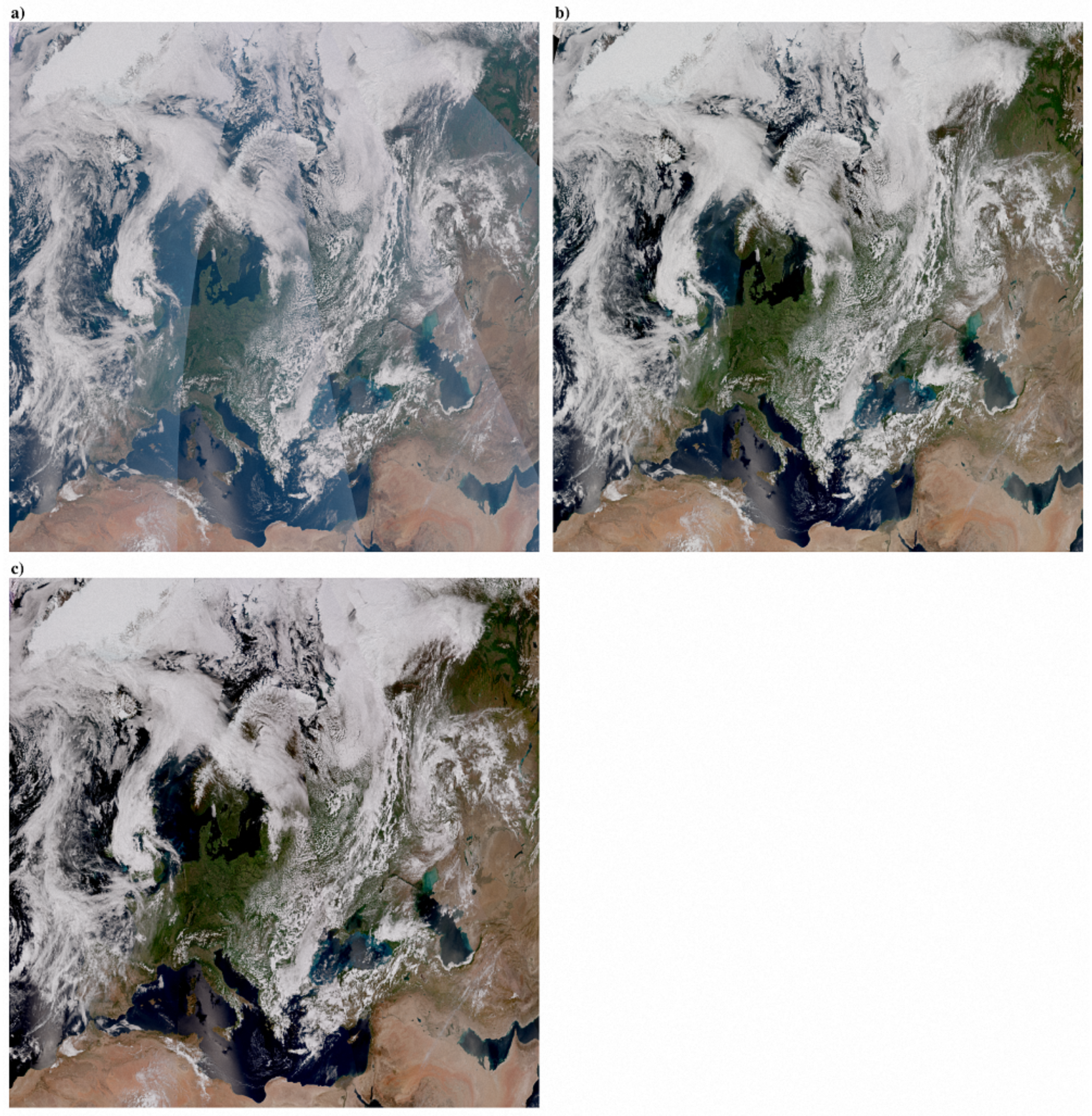
One way to evaluate the consistency of a given technique for satellite image processing is to apply it on data from a series of overlapping polar orbiting satellite overpasses. Creating such a composite scene, pixels with the same or nearly the same surface and atmospheric characteristics but different observation geometry lie side by side along the swath edges. Figure 6 (Supplementary Materials S1) displays a composite created from VIIRS observations of five consecutive Suomi-NPP overpasses over Europe. Individual overpasses are clearly distinguishable on the uncorrected (raw) image a. The interaction of radiation on atmosphere depends strongly on the sun-satellite viewing geometry and there are thus abrupt changes at the edges of swaths. The observations of two consecutive overpasses are separated in time by approximately 102 min (the time it takes for one revolution of a sun-synchronous high-inclination polar orbiting satellite). Provided the surface and atmosphere does not change significantly during this time span these artificial lines separating two passes should disappear after correction by a perfect algorithm, except for cloudy regions, as clouds are usually subject to much faster changes than the state of the surface.
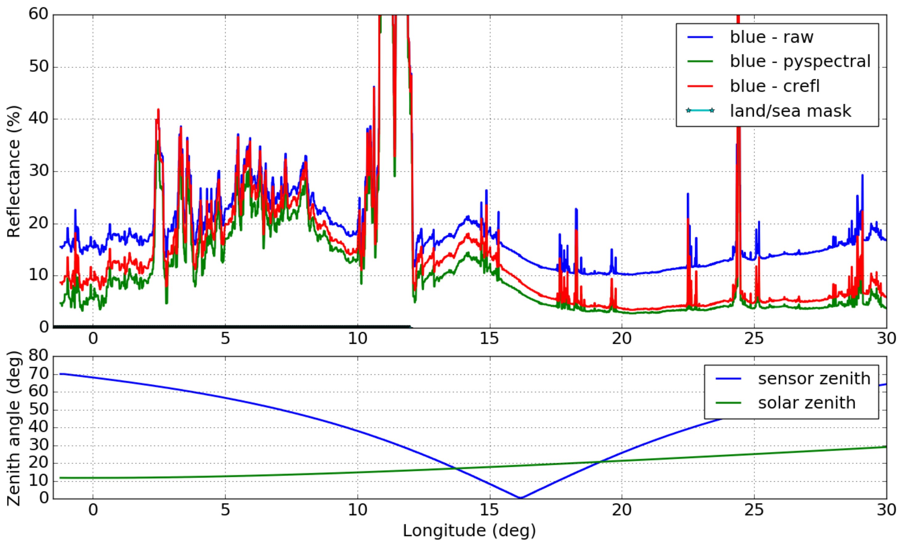
Both corrected images in Figure 6 show improvements in that sense. Also water features due to algae blooming or suspended matter, like the light blueish color seen in the north eastern Caspian Sea and the Black Sea becomes more obvious after correction. There is an overall increase in contrast but overpass edges are still faintly apparent, slightly more distinct in the image corrected by CREFL (b) than in the image processed by the proposed algorithm (c). The image shown in figure c is a result of applying the proposed correction with a US-Standard Atmosphere, and a Continental Average aerosol composition over land areas, and a Marine Clean aerosol composition for water pixels, see Table 2. Figure 7 illustrate how the uncorrected reflectance (here the VIIRS M3 band) increase with increasing atmospheric path length and satellite zenith angle, producing a smile effect. Applying the atmospheric correction presented here removes this smile effect almost completely. The correction is comparable but slightly stronger than the one by CREFL.
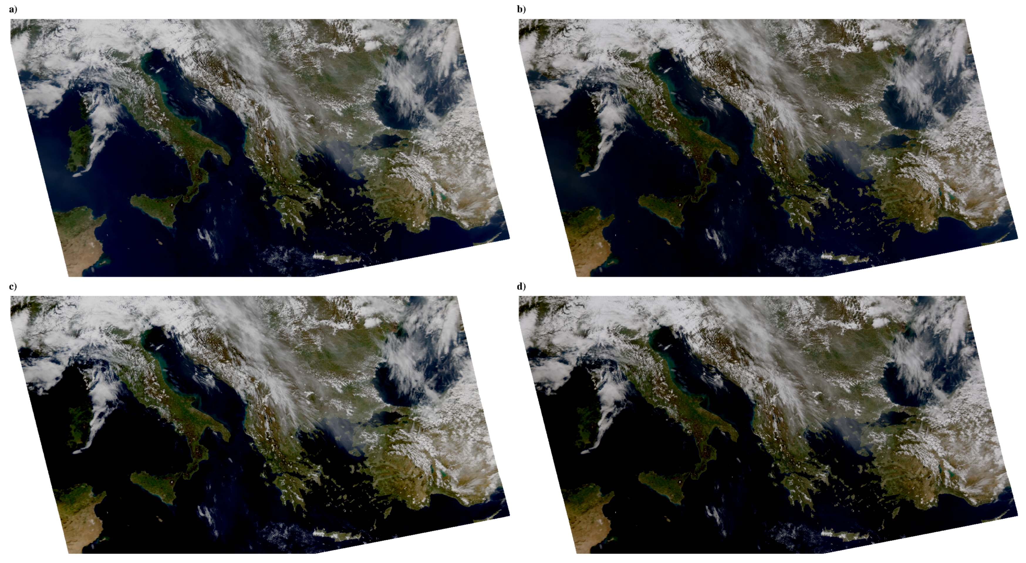
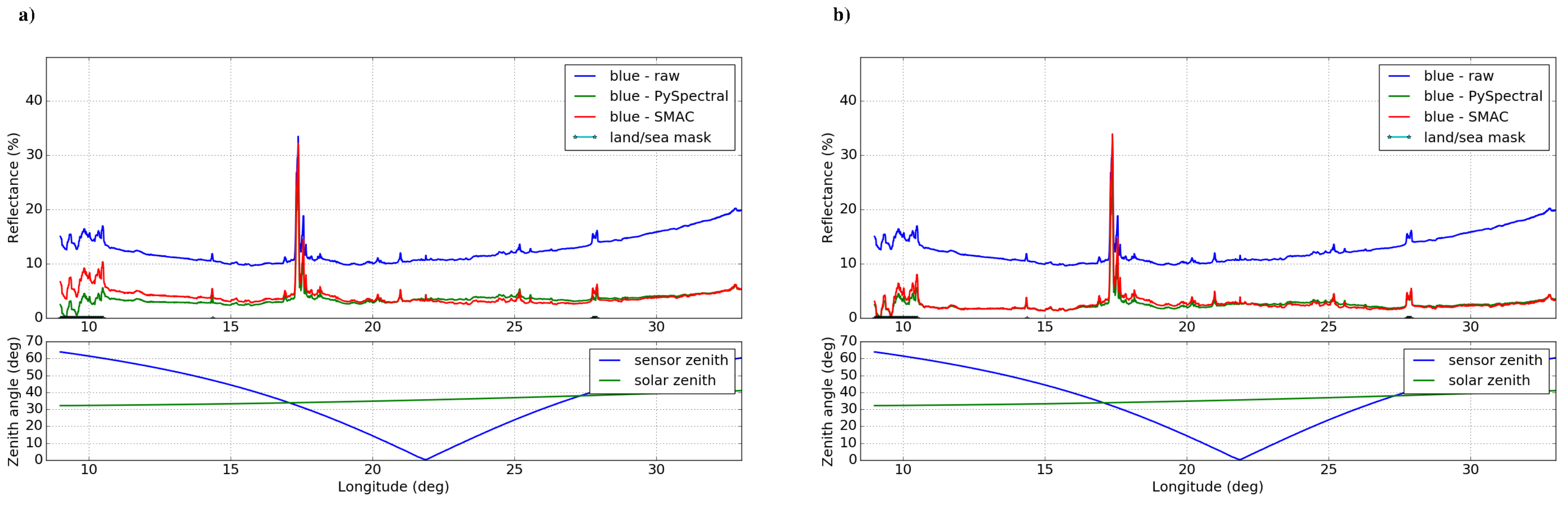
Figure 8 shows an RGB image of the Mediterranean area, observed by the Moderate resolution Imaging Spectroradiometer (MODIS). In a direct inter-comparison with the SMAC algorithm (left column) and without aerosol (upper row), the PySpectral algorithm (right column) provides approximately the same level of detail. The color of the landmass differs slightly between the images. An area south of Corsica looks slight more hazy with SMAC, indicating that SMAC does not completely remove the atmospheric background signal. When adding the marine clean aerosol properties (SMAC was provided with the AOD of the referring aerosol profile), most of the differences disappear or decrease. Looking at the details, a cross section along the 36 degree latitude of uncorrected and corrected reflectance (Figure 9) gives further information. It shows a better agreement between the two algorithms of corrected reflectance in the presence of aerosols (b) than for the aerosol-free scenario (a). Differences in a are most distinct in the western part of the cross section (coinciding with the hazy areas referred to above). The smile-effect (i.e., the reflectance increase towards the edges of the swath as seen in the cross section of the raw data) is more obvious in the aerosol-free correction, and slightly more prominent using SMAC in the western half of the cross section (the hazy area in the image).
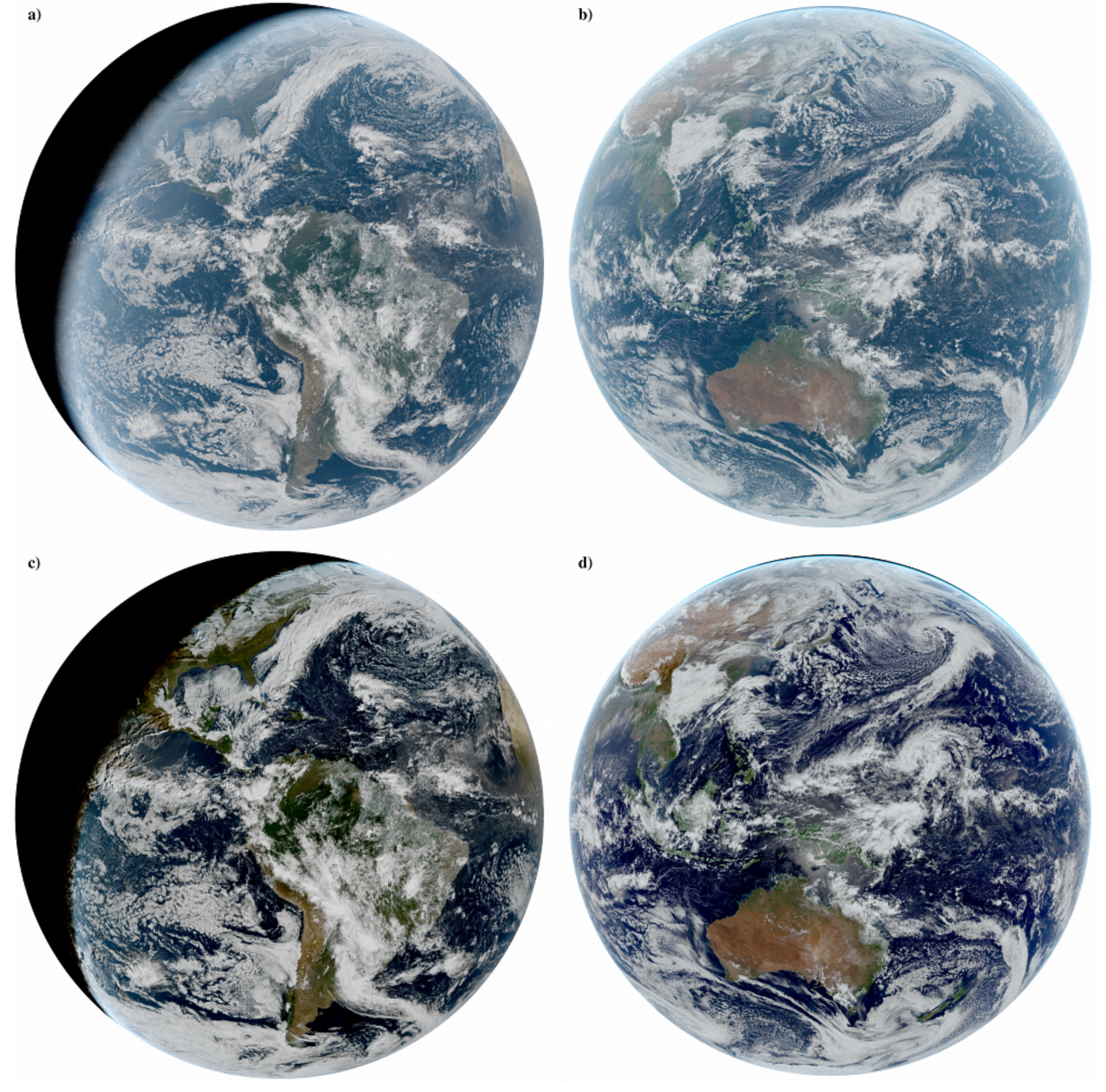
Examples for geostationary satellites are given in Figure 10 (Supplementary Materials S2). A full disk Geostationary Operational Environmental Satellite 16 (GOES-16) image (a and c) and a corresponding Himawari-8 image (b and d) have been processed by the proposed algorithm, using a Tropical gaseous atmosphere, and the Marine Tropical aerosol composition over ocean, and the Continental Average aerosol composition over land. Please note that the Advanced Baseline Imager (ABI) on GOES-16 is lacking a green channel, so to achieve a true color proxy we create a green channel from the red, blue and the NIR band around m. Further, to create the Himawari true color image displayed in Figure 10 we have vegetation boosted the green band by mixing in a bit of the reflectance from the NIR band.
There are no obvious systematic differences between images from both instruments, neither in land, nor in ocean color. Colors are clear and the contrast is high on both images; over a wide range of the disk and thereby over a wide variety of solar and viewing angles. Only close to the edges of the disk is it evident the correction becomes more inefficient. This is expected since the edge itself is a singularity in terms of its geometrical conditions. The pseudo-spherical radiative transfer model, though more adequate than its plane-parallel counterpart, is not aiming to solve for such extreme situations.
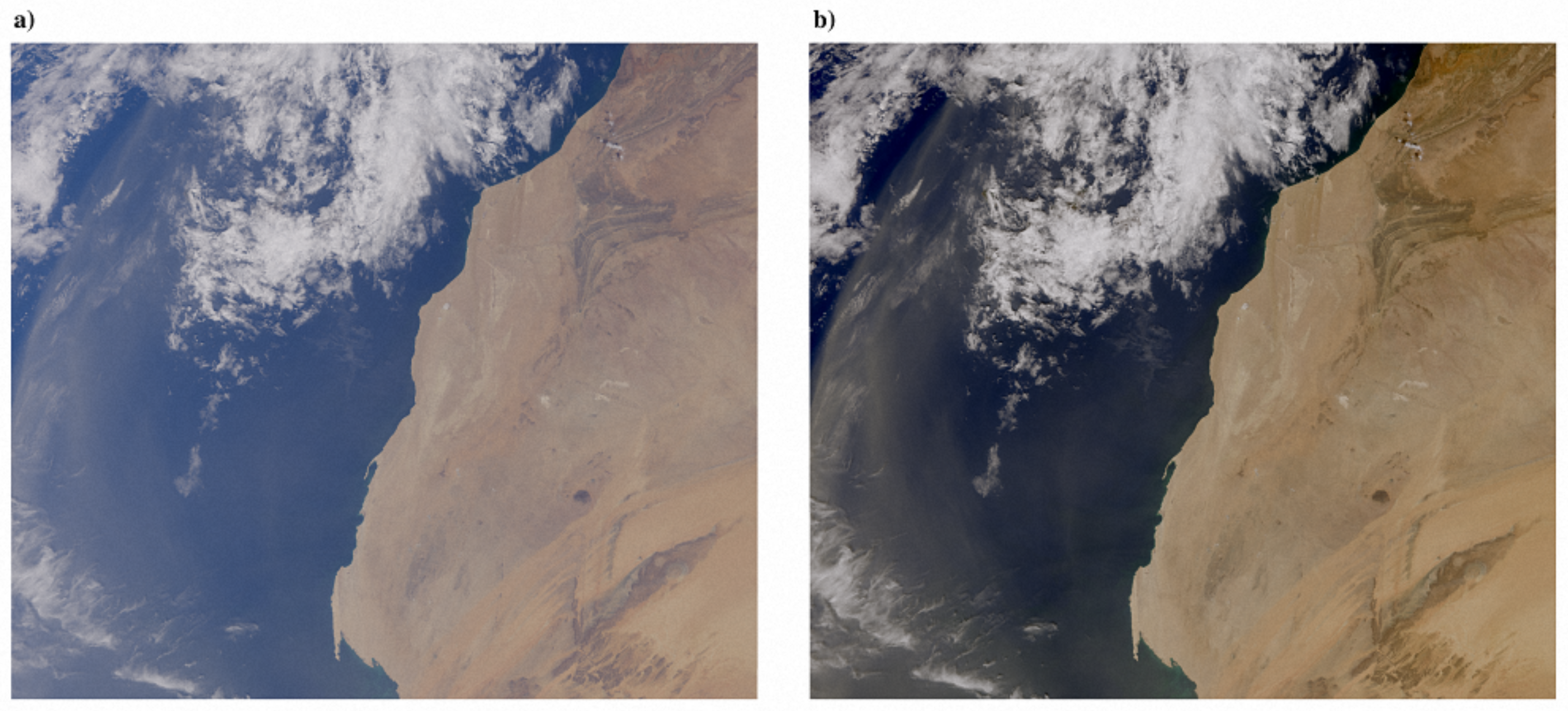
Figure 11 (Supplementary Materials S3) shows a section of east Atlantic ocean and western Africa during a significant desert-dust outbreak in mid October 2017. Compared to the uncorrected image (a), the atmospheric corrected image (b) reveals deeper contrast. It makes it possible to discern more details, as enhanced differences in color provide the possibility to distinguish intuitively between cloud (white), dust (yellowish) and ocean pixels (black). Visualization of clear contours is the key to estimate the propagation velocity from consecutive images. Thus, improved image contrast is a step towards improved forecast of speed and direction of aerosol clouds.
More details on how these examples were created as well as useful program code to process these examples and other satellite data can be found on the Jupyter Notebook viewer [16].
6. Summary and Conclusions
A general method to correct observed TOA reflectance in the visible part of the spectrum from the most dominant atmospheric effects has been presented. The generic approach allows it to be easily applied on any satellite imager operating in the visible spectrum. The method is based on a large database of off-line radiative transfer calculations, assuming a pseudo-spherical atmosphere. In contrast to other methods based on 6S (see [17,18]) and the assumption of a plane parallel atmosphere, the method presented here is more suitable for high solar zenith angles, dominating the high latitudes, and high satellite zenith angles that are constantly present in full-disk Geostationary satellite data. The method seeks to remove the effects of a climatological background atmosphere. Thus the applied correction does not require any ancillary data other than the sun-satellite viewing geometry and the effective wavelength of the spectral band. However, the use of a land-sea mask in order to be able to apply adequate aerosol corrections over both land and sea, is strongly recommended. The correction does not aim to remove the effects of actual and local atmospheric disturbances with enhanced amounts of particles or chemical compounds in the air, for example due to forest fires or dust storms. Rather the removal of the background atmospherical signal will allow improved detection of actual perturbations in the atmosphere as well as surface features on land and in the ocean under normal (unperturbed) conditions.
The method is implemented in PySpectral which is freely available and allows to perform atmospheric correction of satellite imagery in real-time in a few lines of Python code. The LUTs, with the radiative transfer results, and used by PySpectral are available on zenodo.org [19] and downloads automatically when needed. PySpectral integrates with SatPy, another high level Python package of the PyTroll suite of open source software for satellite processing, allowing easy access to a large variety of satellite data and formats.
Corrections of composite satellite scenes demonstrate that the algorithm produces consistent results. This is not only important for this type of images where discontinuities may impede detection of aerosol or surface features, but also for the comparison of images, observed under different geometrical conditions, or with different satellites, where the comparability depends not only on algorithm performance, but also strongly on available spectral channels.
Full-disk imagery from geostationary satellites show homogeneous results over a wide range of solar and satellite viewing angles. Like other methods, at the edges of the geostationary full disk, however, sufficient correction is not possible with this method. In any case, it is questionable whether an analysis under such high viewing angles is meaningful at all.
An example with data from OLCI on Sentinel-3A over western Africa showed how the atmospheric correction scheme can contribute to ease identification of heavy aerosol loads in presence of clouds.
The radiative transfer simulations are done on a set of 6 different standard atmospheres and 10 different aerosol profiles plus one without aerosols, altogether assumed to roughly cover any given observed atmospheric state at any time and place on the earth, from clean marine arctic to polluted continental. The method is generic in the way that it leaves it to the user to apply any one of these atmospheres to a given satellite data set, or combine the results of different aerosol profiles and atmospheres as it is deemed sensible. In this paper, we have used a land-sea mask to apply correction using different profiles and atmospheres over land and sea. Example code showing how to apply such a land-sea dependent atmospheric correction in PyTroll using PySpectral has been demonstrated. As the radiative transfer simulations are valid for a full atmospheric profile from mean sea level to the TOA, pixels over elevated terrain and clouds would be over corrected if applying the corrections from the LUTs unadjusted. The same applies in general to strongly reflective surfaces. Conveniently clouds in particular and to some degree also (snow covered) high terrain are effective reflectors in the short wave. In the method implemented in PySpectral we utilize this and apply a simple linear reduction of the correction over pixels with red band reflectance over .
It would be possible to have a terrain and cloud height dependent adjustment, but this has so far not been implemented in PySpectral, as it is not considered a critical issue for the main applications for which the method and software was developed, namely true color imagery for ocean applications and disaster monitoring and warning including smoke from forest fires and Saharan dust outbreaks. A terrain dependent adjustment would in particular be an improvement to satellite applications over snow and ice free high terrain, and if such needs are found critical for a user application, the generic method presented here, and its open source implementation, allows for such an enhancement.
Supplementary Materials
The following are available online at https://www.mdpi.com/2072-4292/10/4/560/s1.
Acknowledgments
The authors specially wish to thank Abhay Devasthale, SMHI, for valuable and constructive comments and proof reading the draft manuscript. David Hoese, Space Science and Engeneering Center (SSEC), University of Wisconsin-Madison, Madison, USA, has helped during implementation and testing of the method, as well as proof reading the article. The authors are also grateful to the encouragement, comments and suggestions from the anonymous reviewers.
Author Contributions
All three authors contributed to the conception of the paper, the development of the method, data processing, analysis and discussion and the writing of the manuscript. R.S. performed the radiative transfer simulations and the sensitivity study, A.D. and M.R implemented the method in PySpectral and processed the data for the image examples presented.
Conflicts of Interest
The authors declare no conflict of interest.
References
- Vermoté, E.; Vermeulen, A. Algorithm Theoretical Background Document—Atmospheric Correction Algorithm: Spectral Reflectances (MOD09), version 4; NASA, University of Maryland, Department of Geography: College Park, MD, USA, 1999. [Google Scholar]
- Chrysoulakis, N.; Abrams, M.; Feidas, H.; Arai, K. Comparison of atmospheric correction methods using ASTER data for the area of Crete, Greece. Int. J. Remote Sens. 2010, 31, 6347–6385. [Google Scholar] [CrossRef]
- Rahman, H.; Dedieu, G. SMAC: A simplified method for the atmospheric correction of satellite measurements in the solar spectrum. Int. J. Remote Sens. 1994, 15, 123–143. [Google Scholar] [CrossRef]
- Sandmeier, S.; Itten, K.I. A physically-based model to correct atmospheric and illumination effects in optical satellite data of rugged terrain. IEEE Trans. Geosci. Remote Sens. 1997, 35, 708–717. [Google Scholar] [CrossRef]
- Raspaud, M.; Hoese, D.; Dybbroe, A.; Lahtinen, P.; Devasthale, A.; Itkin, M.; Hamann, U.; Rasmussen, L.Ø.; Stigård Nielsen, E.; Leppelt, T.; et al. Pytroll: An open source, community driven Python framework for processing Earth Observation satellite data. Bull. Am. Meteorol. Soc. 2018. submitted. [Google Scholar]
- Putsay, M. A simple atmospheric correction method for the short wave satellite images. Int. J. Remote Sens. 1992, 13, 1549–1558. [Google Scholar] [CrossRef]
- Scheirer, R.; Macke, A. On the accuracy of the independent column approximation in calculating the downward fluxes in the UVA, UVB, and PAR spectral ranges. J. Geophys. Res. Atmos. 2001, 106, 14301–14312. [Google Scholar] [CrossRef]
- Mayer, B.; Kylling, A. Technical note: The libRadtran software package for radiative transfer calculations—Description and examples of use. Atmos. Chem. Phys. 2005, 5, 1855–1877. [Google Scholar] [CrossRef]
- D’Almeida, G.A. On the variability of desert aerosol radiative characteristics. J. Geophys. Res. Atmos. 1987, 92, 3017–3026. [Google Scholar] [CrossRef]
- Léon, J.F.; Derimian, Y.; Chiapello, I.; Tanré, D.; Podvin, T.; Chatenet, B.; Diallo, A.; Deroo, C. Aerosol vertical distribution and optical properties over M’Bour (16.96∘ W; 14.39∘ N), Senegal from 2006 to 2008. Atmos. Chem. Phys. 2009, 9, 9249–9261. [Google Scholar] [CrossRef]
- Stamnes, K.; Tsay, S.C.; Wiscombe, W.; Jayaweera, K. Numerically stable algorithm for discrete-ordinate-method radiative transfer in multiple scattering and emitting layered media. Appl. Opt. 1988, 27, 2502–2509. [Google Scholar] [CrossRef] [PubMed]
- McClatchey, R.; Fenn, R.; Salby, J.; Volz, F.; Garing, J. Optical Properties of the Atmosphere (Environmental Research Papers), 3rd ed.; Technical Report; Air Force Cambridge Research Laboratory: Cambridge, MA, USA, 1972; Volume 411. [Google Scholar]
- Hess, M.; Koepke, P.; Schult, I. Optical Properties of Aerosols and Clouds: The Software Package OPAC. Bull. Am. Meteorol. Soc. 1998, 79, 831–844. [Google Scholar] [CrossRef]
- Shettle, E.P. (Ed.) Models of Aerosols, Clouds, and Precipitation for Atmospheric Propagation Studies. In Proceedings of the AGARD, Atmospheric Propagation in the UV, Visible, IR, and MM-Wave Region and Related Systems Aspects Conference, Copenhagen, Denmark, 9–13 October 1989. [Google Scholar]
- Eastwood, S.; Dybbroe, A.; Scheirer, R.; Håkansson, N.; Godøy, Ø. OSI-SAF/NWC-SAF Federated Activity on Cloud and Ice Masking in Polar Conditions—Final Report; Technical Report; EUMETSAT: Darmstadt, Germany, 2016. [Google Scholar]
- Jupyter Notebook Viewer. Available online: https://nbviewer.jupyter.org/github/pytroll/pytroll-examples/tree/master/pyspectral/ (accessed on 2 February 2018).
- Vermoté, E.; Tanré, D.; Deuze, J.; Herman, M.; Morcrette, J. Second Simulation of the Satellite Signal in the Solar Spectrum: An overview. IEEE Trans. Geosci. Remote Sens. 1997, 35, 675–686. [Google Scholar] [CrossRef]
- Vermoté, E.; Tanré, D.; Deuze, J.; Herman, M.; Morcrette, J. Second Simulation of the Satellite Signal in the Solar Spectrum; User Guide Version 2; Dept. of Geography, Univ. of Maryland, NASA-Goddard Space Flight Center: Greenbelt, MD, USA, 1997; p. 53. [Google Scholar]
- PySpectral Atmospheric correction Look Up Tables. Available online: https://doi.org/10.5281/zenodo.1205534 (accessed on 22 March 2017).
Figure 1.
Conceptual light beams to illustrate the contribution of different information sources to the satellite measurement (see [6]). Part a typifies all beams, that are reflected into space without any contact to the surface. Sketch b represents beams, which are reflected by the surface without atmospheric interaction, and so on. Pure surface information is only transported to the satellite if there is no atmospheric interaction after surface reflection (b, c and partly f, pictured by the dashed path).

Figure 2.
Contour plot of simulated (with LibRadtran [8]) TOA reflectance at 672 nm wavelength for a given Aerosol distribution and constant sun-viewing geometry. Solar zenith angle = , viewing zenith angle = . Aerosol type is mineral dust, optical properties from d’Almeida [9], vertical profile according to Leon et al. [10]. This Figure shows three types of pattern: (I) Reflection increases with increasing aerosol optical thickness (AOT), this is typical for dark surface. (III) Reflection decreases with increasing AOT (very bright surface). (II) Over medium range surface albedo, reflection decreases with increasing AOT up to a certain amount of AOT, where after it decreases. Details determined by vertical distribution of aerosols, absorption coefficient, scattering coefficient and scattering phase function. This pattern changes with atmospheric composition and geometrical settings.

Figure 3.
Illustration of the expected error (a value of 1 means that results of plane-parallel and pseudo spherical simulation are identical) due to assumption of plane-parallel atmosphere. Displayed are ratios of simulated TOA reflections from plane-parallel to the pseudo spherical assumptions for the AVHRR 0.6 m channel (a) and the AVHRR 0.9 m channel (b).

Figure 4.
Examples of spectral TOA reflection by gases and aerosols (Just light-beams that did not reach the surface) at a solar zenith angle of , a viewing zenith angle of and an azimuth difference of . Aerosol-free atmosphere and continental aerosols (a), aerosol-free atmosphere and marine-type aerosols (b). Note the dip around 760 nm, which is due to absorption in the oxygen A-band.

Figure 5.
Relative spectral responses for the low resolution (M-bands) blue, green and red bands of the VIIRS sensor on board the Suomi-NPP platform. The central wave lengths (dashed line) and the “Rayleigh weighted” effective wavelengths (solid line) are shown as well.
Figure 5.
Relative spectral responses for the low resolution (M-bands) blue, green and red bands of the VIIRS sensor on board the Suomi-NPP platform. The central wave lengths (dashed line) and the “Rayleigh weighted” effective wavelengths (solid line) are shown as well.

Figure 6.
Suomi-NPP Visible Infrared Imaging Radiometer Suite (VIIRS) true color RGB composite scene from 27 May 2017. Images from five consecutive overpasses are overlayed on top of each other. Raw uncorrected data (a), data corrected by CREFL [1] (b), and data corrected by PySpectral (proposed algorithm) (c).

Figure 7.
Cross section in one VIIRS orbit from Figure 6 along the 33 degree latitude, from northern Algeria in the west over Tunisia and into the Mediterranean Sea ending a bit north of Alexandria, Egypt. The upper panel show the uncorrected blue (M3) band reflectance (blue) and the corresponding reflectance according to PySpectral (green) and CREFL (red). The lower panel show the satellite sensor and solar zenith angles. The western part of the cross section until around 12 degrees east is over land, and the rest is over water. An area of sun glint seen around 14 degrees east, also visible in Figure 6. The cross section is mostly cloud free over sea with a few cloud patches. The land part of the data arr affected by a pronounced band of clouds over Tunisia (10–12 degrees east) and a few scattered and thinner clouds west of that.

Figure 8.
MODIS scene from 30 March 2016, 11:43 UTC over the eastern Mediterranean region. Left column: Atmospheric correction by the SMAC algorithm (see [3]), Right column: Atmospheric correction using the proposed algorithm implemented in PySPectral. Top row: Without aerosols. Bottom row: With marine clean aerosol profile (PySpectral) and (SMAC).

Figure 9.
A detail view of Figure 8. Cross section along the 36 degree latitude without aerosol (a) and with marine clean aerosol (b).
Figure 9.
A detail view of Figure 8. Cross section along the 36 degree latitude without aerosol (a) and with marine clean aerosol (b).

Figure 10.
Two full-disk true color scenes. The first is from ABI on Geostationary Operational Environmental Satellite (GOES) 16 from 14 January 2018 14:00 (uncorrected (a) and corrected (c)). And the second from Advanced Himawari Imager (AHI) on Himawari-8, from 7 February 2018 03:00 (uncorrected (b) and corrected (d)).

Figure 11.
Sentinel-3A Ocean and Land Color Instrument (OLCI) true color image from 15 October 2017 over western Africa (Western Sahara, Mauritania and southern Morocco) and adjacent Atlantic Ocean. Displayed are raw data (a) and atmospheric corrected data (b). Correction was performed using a tropical atmospheric profile, and a marine tropical aerosol profile over sea and desert aerosol profile over land. An outbreak of heavy loads of Saharan dust over the Atlantic Ocean is more clearly discernible in the corrected image to the right.


Table 1.
Percental contribution to TOA reflection for sketches shown in Figure 1. Calculations are done for mid-latitude summer profile at 0.55 m wavelength for varying solar zenith angle and surface albedo.
Table 1.
Percental contribution to TOA reflection for sketches shown in Figure 1. Calculations are done for mid-latitude summer profile at 0.55 m wavelength for varying solar zenith angle and surface albedo.
| Albedo | a | b | c | d | e | f | |
|---|---|---|---|---|---|---|---|
| 15 | 0.05 | 4.31 | 3.75 | 0.18 | 0.40 | 0.02 | 0.02 |
| 15 | 0.1 | 4.31 | 7.50 | 0.35 | 0.79 | 0.04 | 0.08 |
| 15 | 0.5 | 4.31 | 37.49 | 1.77 | 3.96 | 0.19 | 2.10 |
| 30 | 0.05 | 4.79 | 3.71 | 0.20 | 0.39 | 0.02 | 0.02 |
| 30 | 0.1 | 4.79 | 7.42 | 0.39 | 0.78 | 0.04 | 0.08 |
| 30 | 0.5 | 4.79 | 37.11 | 1.95 | 3.92 | 0.21 | 2.09 |
| 60 | 0.05 | 8.01 | 3.45 | 0.33 | 0.36 | 0.03 | 0.02 |
| 60 | 0.1 | 8.01 | 6.89 | 0.65 | 0.73 | 0.07 | 0.08 |
| 60 | 0.5 | 8.01 | 34.47 | 3.26 | 3.65 | 0.35 | 2.02 |
Table 2.
Variations and range of parameters for radiative transfer simulations. The number in brackets give the optical thickness at 550 nm of the referring profile.
Table 2.
Variations and range of parameters for radiative transfer simulations. The number in brackets give the optical thickness at 550 nm of the referring profile.
| Parameter | Values |
|---|---|
| Atmospheric Profile | Subarctic Summer (0.128), Subarctic Winter (0.13), Midlatitude Summer (0.128), |
| Midlatitude Winter (0.131), Tropical (0.124), US-Standard Atmosphere (0.128) | |
| Background Aerosol | Antarctic (0.032), Continental Clean (0.052), Desert (0.276), Marine |
| Polluted (0.171), Continental Average (0.12), Continental Polluted (0.263), | |
| Marine Clean (0.163), Marine Tropical (0.075), Rural (0.162), Urban (0.536) | |
| Wavelength | 400 to 800 nm in 5 nm steps |
| Solar Zenith Angle | 0., 36.87, 48.19, 55.15, 60., 63.61, 66.42, 68.68, 70.53, 75.52, 80.41, |
| 82.82, 84.26, 86.18, 87.71 | |
| Observation Zenith Angle | 0., 36.87, 48.19, 55.15, 60., 63.61, 66.42, 68.68, 70.53 |
| Azimuth Difference | 0 to 180 in 10 degree steps |
© 2018 by the authors. Licensee MDPI, Basel, Switzerland. This article is an open access article distributed under the terms and conditions of the Creative Commons Attribution (CC BY) license (http://creativecommons.org/licenses/by/4.0/).
Share and Cite
MDPI and ACS Style
Scheirer, R.; Dybbroe, A.; Raspaud, M. A General Approach to Enhance Short Wave Satellite Imagery by Removing Background Atmospheric Effects. Remote Sens. 2018, 10, 560. https://doi.org/10.3390/rs10040560
AMA Style
Scheirer R, Dybbroe A, Raspaud M. A General Approach to Enhance Short Wave Satellite Imagery by Removing Background Atmospheric Effects. Remote Sensing. 2018; 10(4):560. https://doi.org/10.3390/rs10040560
Chicago/Turabian StyleScheirer, Ronald, Adam Dybbroe, and Martin Raspaud. 2018. "A General Approach to Enhance Short Wave Satellite Imagery by Removing Background Atmospheric Effects" Remote Sensing 10, no. 4: 560. https://doi.org/10.3390/rs10040560
Note that from the first issue of 2016, this journal uses article numbers instead of page numbers. See further details here.