Hydrological Effects of Vegetation Cover Degradation and Environmental Implications in a Semiarid Temperate Steppe, China

Abstract

Studying the impact of vegetation dynamics on hydrological processes is essential for environmental management to reduce ecological environment risk and develop sustainable water management strategies under global warming. This case study simulated the responses of streamflow to vegetation cover degradation under climate variations in the Xilin River Basin in a semi-arid steppe of northern China. The snowmelt and river ice melting processes in the Soil and Water Assessment Tool (SWAT) were improved to estimate the changes in streamflow under multiple scenarios. Results showed that the improved SWAT simulations matched well to the measured monthly streamflow for both calibration (determination coefficient R² = 0.75 and Nash–Sutcliffe E_NS = 0.67) and validation periods (R² = 0.74 and E_NS = 0.68). Simulations of vegetation change revealed that obvious changes occurred in streamflow through conversion between high and low vegetation covers. The reductions in vegetation cover can elevate streamflow in both rainfall and snowmelt season, but the effects are most pronounced during the rainfall seasons (i.e., the growing seasons) and in drier years. These findings highlight the importance of vegetation degradation on modifying the hydrological partitioning in a semi-arid steppe basin. We conclude that in a particular climate zone, vegetation cover change is one of the important contributing factors to streamflow variations. Increases in streamflow in water-limited regions will likely reduce the effective water content of soil, which in turn leads to further degradation risk in vegetation. Therefore, vegetation cover management is one of the most effective and sustainable methods of improving water resources in water-constrained regions.

1. Introduction

Terrestrial vegetation plays a crucial role in controlling catchment water balance. Studying the impact of vegetation cover change on streamflow can help water resource managers to develop sustainable management strategies. Vegetation modulates and sustains evapotranspiration (ET) and precipitation (P). Without vegetation, the terrestrial water cycle would be much slower because of smaller ET losses and lower precipitation rates. Land regions lose their rainwater input either as ET or as surface and groundwater runoff [1]. The amount of water that the ground absorbs also will depend on the land cover. Vegetation impacts the speed of water that will move across a surface. More vegetation leads to slower flowing water. Arid and semi-arid regions cover 41% of the Earth's land surface and contain 38% of the human population [2]. These regions are more ecologically vulnerable and sensitive to climate change and human activities. It is a critical challenge to achieve and maintain ecosystem health in these regions [3]. Understanding the connection between vegetation degradation and hydrological processes under global climate change is essential for quantifying the likely consequences of climate change and human activities on grassland ecosystems and achieving long-term grassland ecosystem sustainability in semi-arid watersheds.

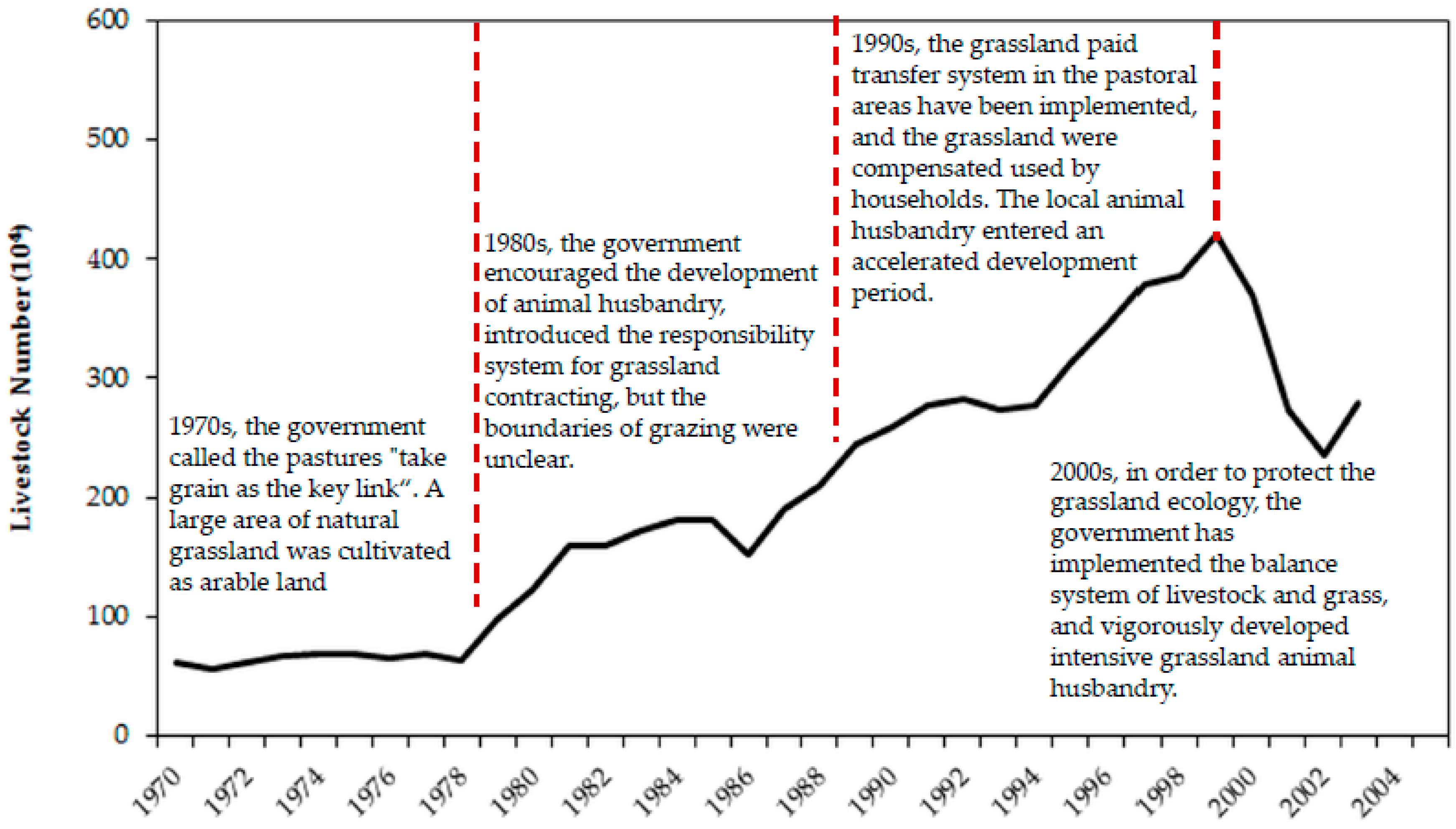
Overgrazing and land cover changes often lead to natural grassland ecosystem deterioration and degradation of catchments in arid and semi-arid regions [4,5,6]. In the Inner Mongolian Plateau of China, land cover change and grassland overgrazing have been recognized as the key causes for the declines of grassland cover and quality, loss of biological diversity and degradation of ecosystem functions [7,8]. Vegetation degradation due to overgrazing and land cover changes affects various hydrological processes, such as interception, infiltration and ET, thereby influencing runoff generation. However, the impacts of vegetation changes on hydrological processes vary in space and time. Little is known in many catchments about the effects of specific land cover types on runoff production, streamflow and water balance closure [9].

Numerous studies have attempted to evaluate the hydrological effects of vegetation dynamics and land cover changes using different methods, such as observation experiments [10], remote sensing products and a statistic-based model [11]. Li et al. [12] investigated the underlying causes of satellite-derived vegetation change and subsequent impacts on runoff in the Northern Shaanxi Loess Plateau. Zhang et al. [13] established a relationship between the change in the landscape parameter and vegetation change using the Budyko equation and quantified the impact of vegetation change on the regional hydrological cycle. However, traditional field experiments are generally constrained to the field scale, and the site level studies may be sensitive to the specific climatic and soil condition [14]. Remote sensing products have some limitations to distinguish vegetation cover classes in arid and semi-arid areas due to their poor and scattered vegetation cover [15]. The physically-based distributed ecohydrological model provided mechanistic and quantitative tools to investigate the connection between vegetation degradation and changes in hydrological processes under global climate change. The Soil and Water Assessment Tool (SWAT) [16] is such a model that utilizes a plant growth module to simulate many types of land cover [17]. As a process-based model, SWAT can be extrapolated to a broad range of conditions that may have limited observations. Therefore, it is widely used to study the impacts of environmental change for a wide range of scales and environmental conditions across the globe [17,18,19].

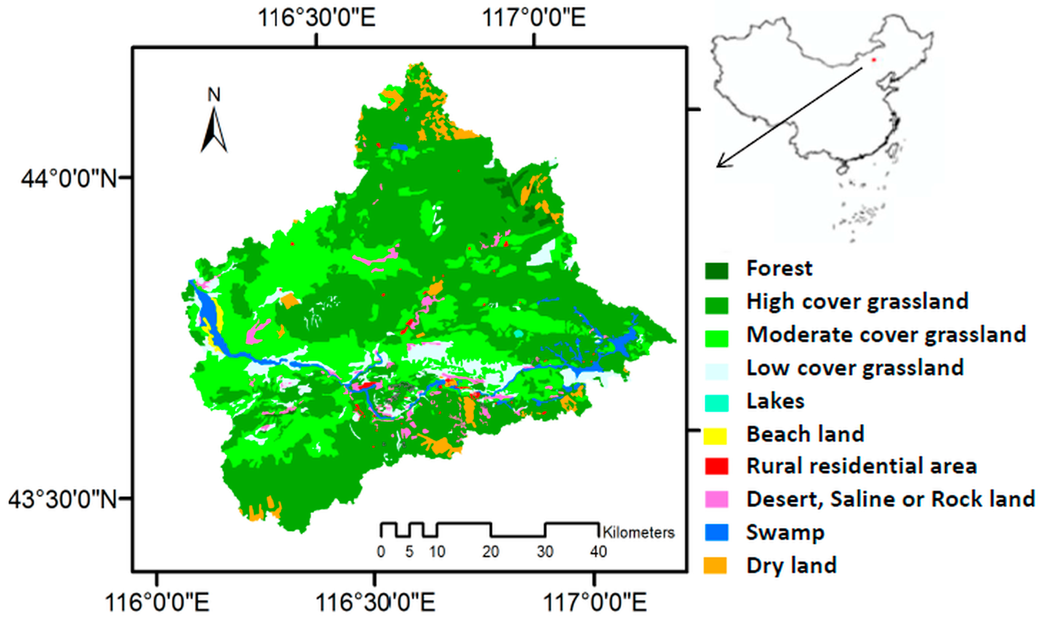
The Xilin River Basin (XLRB) is one of the few well-preserved areas of the Inner Mongolia grassland in northern China. This region has uneven distributions of both water and heat and, thus, large variations in primary productivity and hydrologic regimes [8]. The runoff yield mechanism in the inland river basin is complex, especially for those basins, such as the XLRB, located in semi-arid regions [20]. During the past three decades, due to adverse environmental conditions and intensified human activities (e.g., overgrazing and coal mining), the grassland ecosystem in this region has suffered from severe deterioration [11].

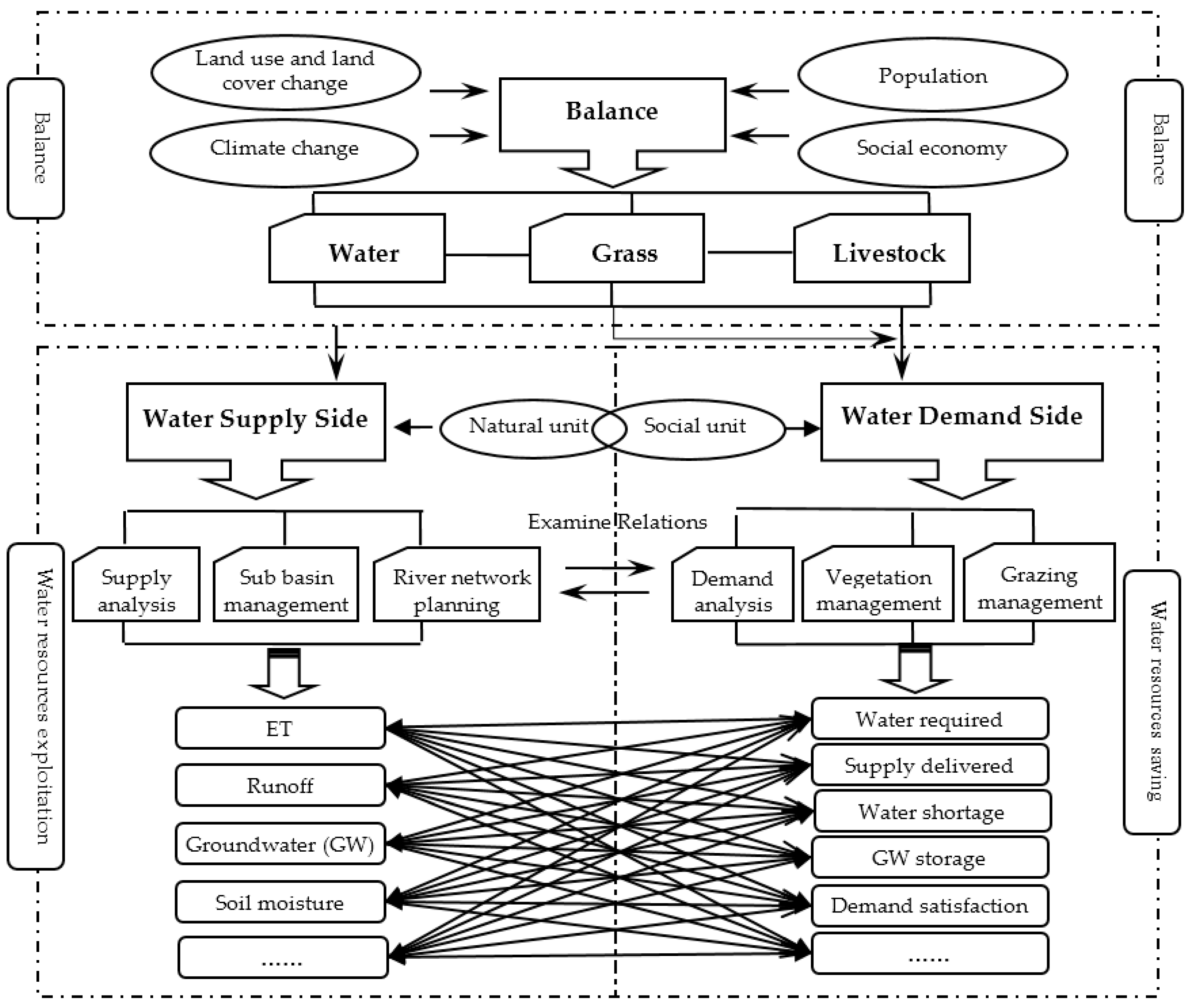
This study aimed at understanding the ecohydrological responses of a water-limited environment to climate changes and human activities using long-term ecohydrological simulation with the SWAT model. The specific objectives of this case study were to explore the following questions: (1) to setup and improve the SWAT model based on understanding the specific hydrological processes of the XLRB; (2) to simulate the consequences of vegetation cover on streamflow under multiple scenarios using improved SWAT; (3) to explore the relationships between vegetation cover and regional water balance. These objectives will be achieved by defining scenarios for changes in vegetation cover inputs to the SWAT model. The results contribute to the in-depth understanding of the mechanism of degradation and restoration of grassland ecosystem and regional biophysical and physiological processes under global climate change, as well as provide critical information to develop methods and strategies towards sustainable development in the study basin and beyond.

2. Materials and Methods

2.1. Location and Climate

The XLRB is located in the central part of the Eurasian Steppe with a typical temperate steppe representing the major native grasslands of Inner Mongolia in northern China. The Xilin reservoir is located in the main stream of Xilin River, which is 9 km away from Xilinhot City. In this paper, the study region is above the reservoir dam site with areas of 3852 km² (43°24′ N–44°08′ N, 116°02′ E–117°16′ E), accounting for 37.4% of the whole of XLRB (Figure 1, Figure 2 and Figure 3).

The XLRB is in the temperate semi-arid continental monsoon climate zone. The annual precipitation is about 300 mm with large intra-annual variability, and about 80% of that falls mainly in summer (June–September). The annual mean temperature is 2.4 °C with large annual and daily temperature fluctuations. Recorded annual extreme maximum and minimum temperatures are 39.9 °C and −42.4 °C, respectively. The freezing period is as long as five months, which is one of the coldest regions in North China. The Xilin River is characterized by a spring flood regimes, which is mostly related to snowmelt and permafrost melting in April. It has a low surface runoff depth of 4.63 mm per year due to very high evaporation with annual pan evaporation of 1904 mm and, hence, a negative water balance. Nevertheless, the surface runoff is very important for the maintenance of the grassland ecosystem [11].

The vegetation types in this region include various formations of typical steppes, meadow steppes and desert steppes. However, the grassland showed a degradation trend during the past three decades. Before the year 2000, an accelerated degradation process has been observed, and the most serious and intensive degradation occurred in the 1990s [21,22], with a decrease by 65.9% in the meadow area (high cover) and 13.8% in the typical steppe area (moderate cover) and an increase by 56.1% in the desert grassland area (low cover) [23]. After 2000, the grassland showed some improvements due to the implementation of a series of local ecological restoration policies and managements [21].

2.2. Improved SWAT Model

The SWAT model provides several options when simulating hydrologic processes, which can be chosen by users based on their data availability. For example, infiltration can be simulated with the curve number (CN) or Green–Ampt method and potential evapotranspiration (PET) with Hargreaves, Priestley–Taylor or Penman–Monteith equation.

In this paper, the traditional SWAT model was applied for the upper part (~3852 km²) of the XLRB first. However, the simulations did not match very well to the measured streamflow. Therefore, we improved the SWAT model based on understanding the specific hydrological processes of XLRB in this study. The following model options were used for all of the XLRB simulations performed in both phases: (1) the curve number method for the partitioning of precipitation between surface runoff and infiltration; (2) the Muskingum method for channel routing; and (3) the Penman–Monteith method for PET.

2.2.1. Specified Vegetation Type

In the SWAT model, there is only one type of grassland with a leaf area index (LAI) of 4.0. In this study, we specified three grassland types in the land use/cover database of the SWAT model according to the vegetation LAI in XLRB [24]. High cover grassland (Pasture with high cover, PSTH) means that its cover is more than 50% with LAI of 4.70; the moderate cover grassland (Pasture with moderate cover, PSTM) is from 20% to 50% with LAI of 1.63; and the low cover grassland (Pasture with low cover, PSTL) is from 5% to 20% with an LAI of 0.65 (

Table 1. Vegetation cover scenarios (km²).

Scenarios	High Cover Area	Moderate Cover Area	Low Cover Area
Baseline (0)	2160	1040	234
Increased (+)	3200	234	0
Decreased (−)	0	2160	1274

).

2.2.2. Improved Snowmelt Module

In XLRB, every year from October to early April in the next year is the snow season with snow cover of about a 20–30-cm depth. The snowmelt runoff in spring accounts for a large proportion of the total annual runoff. However, the simulated snowmelt runoff in SWAT model was much smaller than the measured value. In the SWAT model, the parameters related to snowmelt runoff are SFTMP (mean air temperature at which precipitation is equally likely to be rain as snow/freezing rain, °C), SMTMP (threshold temperature for snow melt, °C), SMFMX (melt factor on 21 June, mm H₂O/day-°C), SMFMN (melt factor on 21 December, mm H₂O/day-°C) and TIMP (snow temperature lag factor). The improvement of simulation for the snowmelt runoff will be limited if only these parameters are calibrated. Therefore, we improved the snowmelt module as follows.

In SWAT, the mass balance for the snow pack is:

Sno_i = Sno_i−1 + R_day − E_sub − Sno_mlt

(1)

where Sno_i is the water content of the snow pack on current i day (mm H₂O), Sno_i−1 is the water content of the snow pack on the i − 1 day (mm H₂O), R_day is the amount of precipitation on a given day (mm H₂O), E_sub is the amount of sublimation on a given day (mm H₂O) and Sno_mlt is the amount of snow melt on a given day (mm H₂O). The amount of snow is expressed as depth over the total hydrologic response unit (HRU) area.

Due to the influences of wind drifting, shading, topography and land cover factors, the snow in XLRB is always concentrated in the upstream river course and swamp basins. The snow accumulation increased snow depth and reduced snow sublimation area and, thus, reserved water in snow. The original SWAT model calculated the change of snow cover according to the areal depletion curve based on the correlation between snow cover extend areas and the amount of snowfall, but this is not suitable for the XLRB. We analyzed the historic observed data of snow and spring flood in the XLRB and found that the spring flood peak can be better simulated if the snowfall were multiplied by a coefficient α.

Sno_i = Sno_i−1 + R_day α − E_sub − Sno_mlt

(2)

where α is the compensation coefficient; see Equation (3). It can be seen that α is inversely proportional to snowfall in the current i winter (snow_i), and proportional to snowfall in the i − 1 winter (snow_i−1). In the actual application in the XLRB, the snow_i should be divided into three levels of <10 mm, 10 mm–20 mm and >20 mm to calibrate β and C, respectively.

$$\alpha =\frac{sno{w}_i+sno{w}_{i-1}\times 0.1}{sno{w}_i}\times \beta +C$$

(3)

where snow_i is snowfall in the current i winter and snow_i−1 is snowfall in the i − 1 winter. β and α are the empirical coefficients that need to be calibrated at different stages based on the snowfall in the current winter. We added a module to input snowfall data into the SWAT model before running the module. In order to guarantee the reliability of the simulation, a preheating period of at least two years was required.

2.2.3. Improved Groundwater Module

The SWAT model simulates two aquifers in each sub-basin. The shallow aquifer is an unconfined aquifer that contributes to flow in the main channel or reach of the sub-basin. The deep aquifer is a confined aquifer. Water that enters the deep aquifer is assumed to contribute to streamflow somewhere outside of the watershed [16].

The water balance for the shallow aquifer is:

aq_sh,i = aq_sh,i−1 + w_rchrg − Q_gw − w_revap − w_deep − w_pump,sh

(4)

where aq_sh,i is the amount of water stored in the shallow aquifer on day i (mm H₂O), aq_sh,i−1 is the amount of water stored in the shallow aquifer on day i − 1 (mm H₂O), w_rchrg is the amount of recharge entering the aquifer on day i (mm H₂O), Q_gw is the groundwater flow, or base flow, into the main channel on day i (mm H₂O), w_revap is the amount of water moving into the soil zone in response to water deficiencies on day i (mm H₂O), w_deep is the amount of water percolating from the shallow aquifer into the deep aquifer on day i (mm H₂O) and w_pump,sh is the amount of water removed from the shallow aquifer by pumping on day i (mm H₂O).

However, some scholars found that significant increases in precipitation will lead to an abnormal maximum streamflow value in the hydrological simulation using the SWAT model. Song and Ma [18] found that in the year with increased precipitation, the abnormal high streamflow value occurred and continued and thereafter affected the simulation results in the next year. Bai et al. [19] also encountered the same problem in the Kaidu River Basin, and their solution was to remove the two years with an abnormally high value. We also found that when the sum of aq_sh,i−1 and w_rchrg was greater than GWQMN (threshold water level in the shallow aquifer for base flow), the simulated runoff was unusually large. This problem can be solved when w_rchrg was multiplied by a coefficient α as follows:

aq_sh,i = aq_sh,i−1 + w_rchrg,sh α − Q_gw − w_revap − w_deep − w_pump,sh ((aq_sh,i−1 + w_rchrg) > GWQMN)

(5)

where 0.95 < α < 1 and α needs to be calibrated.

2.2.4. Improved Seasonal Permafrost Module

The XLRB is located in the seasonal permafrost regions, and its frozen period is up to six months from November to early April in the next year. The thickness of the permafrost is up to 3.2 m. In existing studies, it is generally believed that the hydrological process in permafrost is complicated, and permafrost increases the water storage capacity of soil [25]. In the XLRB, the phenomenon of ‘frozen to the bottom’ often occurred in the river from early December to the end of March in the next year. During this period, shallow groundwater cannot supply the river channel, and the runoff in the river is zero. When permafrost melts in April, runoff increases dramatically in a short period, and storm stream occurs.

The SWAT model calculates soil temperature in different soil layers through the soil temperature module. When the temperature of the second soil layer is below 0 °C, the SWAT model considers the start of the permafrost process. At this time, the precipitation interception by the soil surface layer increased, and the process in which soil water leaked downward stopped. However, the process in which the shallow aquifer supplied the river channel still existed. Apparently, the SWAT model did not consider the phenomenon of ‘frozen to the bottom’ in this basin. We also found that the soil frozen period is very consistent with the dry season in the XLRB. Based on this, we developed the module of water storage in frozen soil. The main equation is as follows:

$$\{\begin{array}{c}\mathrm{g}{w}_q=0(soi{l}_{tem}<0)\\ w_{frz}=\alpha \left(w_{rchrg}-w_{deep}\right)\times \left(1-\exp \left(alpha\_bf\right)\right)(soi{l}_{tem}<0)\end{array}$$

(6)

where gw_q is the supplementary amount of the groundwater recharge to the river channel, w_frz is the water storage when permafrost occurred, alpha_bf is the regression coefficients of the baseflow, soil_tmp is the soil temperature of the second layer, α is a constant that needs to be calibrated and the definition of w_rchrg and w_deep is the same as Equation (4).

2.3. Data

In this paper, the DEM (digital elevation model, 1:250,000), soil types map (1:1,000,000) and land cover maps (1996 and 2000, 1:100,000) were provided by the Environmental and Ecological Science Data Center for West China (Figure 1, Figure 2 and Figure 3).

2.3.1. Land Use and Land Cover Data

The main land cover in this basin is grassland, accounting for more than 90% of total area (Figure 1). In 2000, the high cover grassland area (cover ≥ 50%), moderate (20% ≤ cover ≤ 50%) and low (5% ≤ cover ≤ 20%) accounts for 57%, 28% and 6% of the whole basin area, respectively. Over the past three decades, the XLRB suffered dramatic vegetation degradation characterized by decreases in high and moderate cover grassland and increases in shrub, desertification land and saline land [23,26].

2.3.2. Soil Data

The soils in this area range from dark chestnut soils, chernozem, dune sand to light chestnut soils. The soil database in SWAT is based on the simplified American standard formulated by the USDA (Figure 3). China has completed two national soil surveys (1958–1960, 1979–1985), respectively adopting the system of the Soviet Union (Kaczynski system) and international system [27]. The soil classification data [28] and soil database used in this paper are obtained from Nanjing Institute of Soil Science, Chinese Academy of Sciences [29], which adopted the international soil particle size grading standard. Before applying to the SWAT model, it has been transformed into the American standard. There are many methods to convert soil particle size. Due to the relatively smaller error, the cubic spline interpolation method [30] was used to carry out interpolated calculation. The soil-plant-atmosphere-water (SPAW) model [31] was used to calculate parameters including the available water capacity of the soil layer, (SOL_AWC), the soil moist bulk density (SOL_BD) and the soil saturated hydraulic conductivity (SOL_K) to build the soil database for SWAT model.

2.3.3. Meteorological and Hydrologic Data

There is no weather observation station in the XLRB. The nearest weather stations are Xilinhot station (43°57′ N, 116°07′ E), West Ujimqin station (44°35′ N, 117°36′ E) and Linxi station (43°36′ N, 118°04′ E). We collected meteorological data of these three stations during 1958–2012 from the China Meteorological Administration (CMA) and Inner Mongolia Meteorological Bureau, which included daily data of precipitation, maximum and minimum temperature, solar radiation, humidity and wind speed. The inverse square law was used for the interpolation of the observed data in the three stations for the SWAT model input.

The runoff data of the Xilin River were obtained from the Xilinhot Hydrologic station (Figure 2) which included annual data during 1958–2008 and monthly data during 1963–1973, as well as daily data during 1976–1979 and 1991–1994. Due to no water diversion project in the upstream of Xilinhot hydrological station and thus no need for water reduction calculation, the measured runoff series can be used on behalf of the natural runoff series. In this study, the streamflow in the rainfall season was defined as the average value from July to August, and that in the snowmelt season was from March–April.

2.4. Model Evaluation

The coefficient of Nash–Sutcliffe simulation efficiency (E_NS) and the determination coefficient (R²) were used to evaluate the performance of the SWAT model (Equations (7)–(9)). The R² value provides a measure of how well observed outcomes are predicted by the model. The E_NS value indicates how well the plot of the observed versus the simulated values fits the 1:1 line [32]. In addition, we used relative error (R_E) to indicate model bias.

$$E_{NS}=1-\frac{{\sum }_{i=1}^n{(Q_o-Q_p)}^2}{{\sum }_{i=1}^n{(Q_o-Q_{avg})}^2}$$

(7)

$$R^2=\frac{{\left(n\sum Q_o\times Q_p-\sum Q_o\sum Q_p\right)}^2}{(n\sum Q_o^2-{(\sum Q_o)}^2)(n\sum Q_p^2-{(\sum Q_p)}^2)}$$

(8)

$$R_E=\frac{Q_p-Q_o}{Q_o}\times 100\%$$

(9)

where Q_o is observed steam flow, Q_p is simulated steam flow, Q_ave is mean observed steam flow and n is samples.

2.5. Scenarios’ Setup

According to Chen [23] and Yan et al. [21], the XLRB shows decreases in high and moderate cover grassland and increases in low cover areas over the past three decades. Based on this, we set two vegetation cover scenarios to represent improved and degraded vegetation situation (Table 1), and multiple scenarios with vegetation cover change and climate variations (

Table 2. Multiple scenarios with vegetation cover changes and climate variations. P, precipitation.

Scenarios	T (°C)	P (%)	Vegetation	Scenarios	T (°C)	P (%)	Vegetation
S00	0	0	0	S14	+1	0	−
S01	0	0	+	S15	+1	+15	0
S02	0	0	−	S16	+1	+15	+
S03	0	−15	0	S17	+1	+15	−
S04	0	−15	+	S18	+2	−15	0
S05	0	−15	−	S19	+2	−15	+
S06	0	+15	0	S20	+2	−15	−
S07	0	+15	+	S21	+2	0	0
S08	0	+15	−	S22	+2	0	+
S09	+1	−15	0	S23	+2	0	−
S10	+1	−15	+	S24	+2	+15	0
S11	+1	−15	−	S25	+2	+15	+
S12	+1	0	0	S26	+2	+15	−
S13	+1	0	+

). In the baseline, the vegetation cover is that of 2000, and the observed climate is from 1961 to 2010.

3. Results

3.1. Climate and Hydrology Variations

The climate records at Xilinhot Weather Station indicate that there is a drying and warming trend during the past five decades (Figure 4) with precipitation declined at −8.1 mm∙10 a⁻¹ (10 a⁻¹ represents per a ten-year period) and temperature increased at 0.42 °C∙10 a⁻¹. The annual mean runoff depth is 4.63 mm with a slow decline of 0.39 mm∙10 a⁻¹ (p > 0.05) during the whole five decades, but there is a significant decreasing trend during 1958–1990 (p < 0.05), a significantly increasing trend (p < 0.05) in the 1990s and a significant decline (p < 0.05) in the 2000s. The runoff coefficient declined since the 1960s and fell to the lowest during the 1980s, then increased in the 1990s and decreased again in the 2000s (Figure 5, insert).

Seasonal change of runoff shows that a bimodal type runoff process results from snowmelt, permafrost melt and precipitation (Figure 5, insert). The runoff in April is the highest peak value (1.67 mm); the amount of that accounts for about 32% of the total annual runoff. In May, the snow and permafrost melt completely, and the runoff mainly comes from rainfall. At the same time, grass grows with the rising temperature, and runoff decreases gradually with increasing ET [4]; the runoff reached a relatively low value of about 0.44 mm in June. The second peak flow occurred in August (0.63 mm), less than the spring flood peak. From December to March in the next year, the phenomenon of ‘frozen to the bottom’ occurs, and the runoff is zero.

The double mass curve (Figure 5) showed that compared with the 1960s (Q/P = 0.019, Q is mean runoff), the accumulated runoff has an obvious deviation during the 1970s (Q/P = 0.016) and 1980s (Q/P = 0.013), which represents a decrease in the runoff coefficient. However, the slope of the accumulated curve in the 1990s is back to the 1960s, with an increase in the runoff coefficient (Q/P = 0.021).

3.2. Calibration and Validation of the Improved SWAT Model

The sensitivity of 26 parameters related to the runoff was analyzed and sorted using the LH-OAT sensitivity analysis tool [32] in the SWAT model. Nine parameters influenced the simulated runoff results greatly, including CN2, GWQMN, REVAPMN, ALPHA_BF, GW_DELAY, SMFMX, SMFMN, TIMP and RCHRG_DP, selected for calibration manually (

Table 3. Hydrologic calibration parameters and values for the Xilin River Basin (XLRB).

Parameters	Descriptions	Initial Estimates	Calibrated Value
CN2	Curve number for moisture Condition II	a 1	−44
GWQMN	Threshold water level in the shallow aquifer for baseflow (mm)	0	+3.95
REVAPMN	Threshold water level in the shallow aquifer for “revap” 2 or percolation to the deep aquifer (mm)	1	+2.98
ALPHA_BF	Baseflow recession constant	0.048	+0.032
GW_DELAY	Delay time for aquifer recharge (days)	31	+469
SMFMX	Melt factor on 21 June (mm/day-°C)	4.5	−3.1
SMFMN	Melt factor on 21 December (mm/day-°C)	4.5	−3.2
TIMP	Snow temperature lag factor	1	−0.78
RCHRG_DP	Aquifer percolation coefficient	0.05	−0.01

¹ a represents initial SCS runoff curve number, the value changed in different HRUs; ² “revap “means water in the shallow aquifer returning to the root zone in response to a moisture deficit during the time step (mm H₂O).

).

After modification of the groundwater module, frozen soil module, as well as the improved snowmelt module, the simulations matched well to measured monthly streamflow for both the calibration periods (R² = 0.75 and E_NS = 0.67) and validation periods (R² = 0.74 and E_NS = 0.68) (

Table 4. Evaluation of the simulated results using the improved SWAT model during the calibration period (1963–1967) and the validation period (1968–1972).

Improved SWAT Modules	Period	ENS	R2	|RE|
Original simulation results	Calibration	−0.36	0.14	0.48
	Validation	−0.36	0.19	0.47
Improved snowmelt module	Calibration	0.06	0.25	0.12
	Validation	0.25	0.39	0.38
Improved snowmelt, groundwater and frozen soil module	Calibration	0.67	0.75	0.15
	Validation	0.68	0.74	0.11

, Figure 6).

3.3. Response of Streamflow to Climate and Vegetation Change

Using the S00 scenario as the baseline, the simulated largest runoff occurred in S08 with an increase by 84% in streamflow, while the smallest in S19 with a decrease by 76%. Comparison of S06 and S03 with the S00 simulation results, we can see that under the multiple scenarios with fixed temperature and grassland cover, the streamflow increased by 49% when precipitation increased by 15% and reduced by 42% with the rainfall decrease by 15%. In the scenarios of S12, S21 and S00 with fixed precipitation and grassland cover, the streamflow decreased by 21% with temperature increased by 1 °C and reduced by 38% with the temperature increase by 2 °C. In the scenarios of S02, S01 and S00 with fixed temperature and precipitation, the streamflow increased by 29% as a result of seriously degraded vegetation cover and reduced by 13% when the grassland recovered (

Table 5. Streamflow (Q) in different climate variation and vegetation scenarios (1961–2010).

Scenarios	T (°C)	P (%)	Vegetation	Mean Q (m3∙s−1)	Change in Q (%)
S08	0	15	−	0.93	83.9
S17	+1	15	−	0.80	57.5
S06	0	15	0	0.75	49.2
S26	+2	15	−	0.69	35.8
S07	0	15	+	0.68	33.7
S02	0	0	−	0.65	29.4
S15	+1	15	0	0.62	22.4
S16	+1	15	+	0.54	7.7
S14	+1	0	−	0.54	7.3
S24	+2	15	0	0.52	2.0
S00	0	0	0	0.51	0.0
S23	+2	0	−	0.45	−11.1
S25	+2	15	+	0.45	−11.6
S01	0	0	+	0.44	−12.5
S05	0	−15	−	0.41	−19.8
S12	+1	0	0	0.40	−20.6
S13	+1	0	+	0.34	−32.1
S11	+1	−15	−	0.32	−37.4
S21	+2	0	0	0.32	−37.5
S03	0	−15	0	0.29	−41.8
S22	+2	0	+	0.26	−48.0
S20	+2	−15	−	0.25	−50.3
S04	0	−15	+	0.25	−51.3
S09	+1	−15	0	0.21	−57.8
S10	+1	−15	+	0.17	−66.3
S18	+2	−15	0	0.15	−69.4
S19	+2	−15	+	0.12	−76.1

).

In rainfall seasons from July to August (1963–1972), the streamflow increases apparently by 15% with a reduction in vegetation cover compared with the baseline, and increases by 9% in the snowmelt season from March to April (

Table 6. Mean streamflow in the snowmelt season (March–April) and the rainfall season (July–August) (1963–1972).

Year	Baseline S00 (m3∙s−1)		Degraded Vegetation S02 (m3∙s−1)		Increase Rate (%)
	Snowmelt	Rainfall	Snowmelt	Rainfall	Snowmelt	Rainfall
1963	0.56	0.96	0.62	1.06	10	11
1964	0.95	0.83	1.00	0.93	6	13
1965	0.09	0.53	0.12	0.61	32	15
1966	0.15	0.39	0.18	0.45	19	15
1967	0.17	0.77	0.17	0.90	5	18
1968	0.77	0.07	0.77	0.09	−1	27
1969	0.26	1.23	0.34	1.41	30	14
1970	0.55	0.55	0.62	0.63	12	13
1971	1.02	0.47	1.13	0.56	11	19
1972	0.70	0.25	0.80	0.29	14	16
Average	0.52	0.60	0.57	0.69	9	15

). This is mainly because that the rainfall seasons has more vegetation cover than the snowmelt season.

For the periods with small snowmelt (e.g., 1965, 1966), the effects of decreasing vegetation cover on the streamflow are more obvious (32%, 19%, respectively) than those with more snowmelt (e.g., 6% and 11% for 1964 and 1971, respectively). The rainfall streamflow has similar effects with that of snowmelt, i.e., the vegetation effects with less rainfall are more obvious (27% in 1968) than those with more rainfall (e.g., 11% and 14% for 1963 and 1969, respectively) (Table 6).

3.4. Grazing History

Figure 7 shows the livestock number change and management policies during different periods in this basin. By 2000, the number of livestock had grown from 600 thousand to about four million. It was not until 2000 that the livestock number reduced. The government management policy was the main driving force of livestock numbers. Before the year 2000, the main purpose of the government’s management policy was to promote economic development. After 2000, the government began to pay more attention to ecological environment protection, implemented the balance system of livestock and grass, and vigorously developed intensive grassland animal husbandry.

3.5. “Water-Grass-Livestock” Conceptual Framework

We propose a “water-grass-livestock” conceptual framework for integrated watershed management in water-constrained pastures (Figure 8). The management conceptual framework illustrates the point to determine the pasture scale according to the available water resources and to determine the livestock number according to the pasture scale and its carrying capacity, i.e., to keep the balance of “water-grass-livestock”.

4. Discussions

4.1. SWAT Model Improvement

Vegetation is a key component of terrestrial ecosystems and thus mandatory to be considered in integrated models simulating biophysical and hydrological processes [17]. The distributed hydrological SWAT model has become an effective method to analyze the hydrology, ecology and environment of the watershed due to its accurate description of the mechanism of hydrological processes, the clear physical meaning of the parameters and the effective usage of spatial information with remote sensing (RS) and geographic information system (GIS) technology.

However, the original structure and database of the SWAT model is designed based on the hydrological and geographical conditions in agricultural watersheds in North America. The impacts of vegetation changes on hydrological process differ across regions depending on many kinds of changes experienced and the specific response of regional vegetation to those changes, including both climate and human activities, especially in arid and semi-arid regions with less precipitation and large annual and intra-annual variability in precipitation and temperature. All of these characteristics put forward higher requirements for the hydrological model to simulate the water balance accurately. Previous studies [33,34] point out that the SWAT model needs to be improved in the simulation of snowmelt runoff and permafrost processes when applied in cold regions. In this study, we improved the snowmelt, groundwater and frozen soil module of the SWAT model based on understanding the specific hydrological behavior of XLRB. The results show that the improved SWAT model simulations matched well to measured monthly streamflow for both the calibration periods and validation periods. However, at present, our improvement is mainly based on empirical evidence, rather than on the basis of the physical mechanism of the ecohydrological process.

4.2. Relationship between Vegetation and Hydrology

Streamflow is an important indicator of hydrological processes that represents the combined effects of climatic and land surface conditions [3]. This study simulated the consequences of vegetation cover and climate variations scenarios on streamflow using the improved SWAT. The simulation results show that the streamflow is sensitive to both climate variations and vegetation cover changes. The reductions in vegetation cover can elevate the streamflow in the rainfall season (July–August), which is higher than that in the snowmelt season (March–April) with less vegetation cover.

Previous studies suggested that vegetation change may affect greatly the precipitation distribution ratio between actual evapotranspiration and runoff [3]. Gumindoga et al. [9] predicted streamflow for land cover changes in the Upper Gilgel Abay River Basin using TOPography based hydrological MODEL (TOPMODEL) and found that the highest peak flow, as well as the annual streamflow volume varied among the land cover types agriculture, forest and grassland. Li et al. [12] pointed out that more ET from restored vegetation in recent large-scale ecological restoration projects is the primary reason for the reduced runoff coefficient in the Northern Shaanxi Loess Plateau. Liang et al. [3] found the runoff coefficients in flood season and non-flood season were both decreased in China’s Loess Plateau based on a Budyko hydrological model. Yang et al. [35] found a positive correlation between the water balance component (ET/P) and vegetation cover in the Yellow River Basin and the Inland River Basin using the Budyko hypothesis. Wang et al. [11] investigated runoff and vegetation by observation experiments combining RS and GIS technology in the XLRB and found that the total runoff increases continually in the growing season in the last 30 years.

Our simulation findings show that vegetation degradation causes the increase in streamflow, and vegetation restoration reduces streamflow, which are partially consistent with previous studies. The maximum slope of double mass curve and biggest runoff coefficient (Q/P = 0.021) in the 1990s with the most serious grassland degradation situation [21,23] (Figure 5) also supports our simulation results. Boggs and Sun [36] conclude that the effects of vegetation removal on streamflow are most pronounced during the growing seasons. Our results also showed that the reductions in vegetation cover can elevate the streamflow in both rainfall season (July–August) and the snowmelt season (March–April), but the effects of the former appear more obvious due to more vegetation cover in the rainfall season. During the past three decades, decreased precipitation during the flood season in the XLRB as a dominated factor results in the decreasing annual runoff, which were partly offset by increased runoff due to ice and snow melt in warming winter and vegetation cover reductions. Less ET due to degraded vegetation results in increases in streamflow, which will reduce the effective water content of the soil and in turn lead to the degradation in vegetation with combined effects of drying and warming climate in this water-limited region. Long-term monitoring data in this region indicated that soil moisture has dramatically decreased at 50-, 70- and 100-cm depths during the past decades as a result of persistent drought and the change in precipitation patterns [4]; and likely vegetation change. Therefore, ecological and hydrological processes can interact strongly in landscapes, yet these processes are often studied separately [37]. A better understanding of the relationship between vegetation and water balance would help to explain the complicated interactions between climate change, vegetation dynamics and the water cycle [35]. The present study advanced the understanding of the processes of vegetation degradation on streamflow using the improved process-based SWAT model. Study results had important environmental implications for semi-arid inland basins in China and elsewhere with similar environments.

4.3. Relationship between Vegetation and Grazing

In water-limited pastures, attributing the trend in runoff to the changing climate and anthropogenic factors is a topic that is important for future water resource planning and management decisions to ensure sustainable water resource utilization [38]. Our modeling results suggest that vegetation degradation causes increases in streamflow, and vegetation restoration reduces streamflow. Vegetation cover management is one of the most effective methods of improving water resources. A complete vegetation cover helps to reduce soil erosion and flooding through the detention of rainfall by interception, increased infiltration and reduced runoff through enhanced evaporation and evapotranspiration.

A major challenge facing pastoralists in highly variable rangeland environments is balancing animal numbers with forage supply. Overgrazing is a key factor driving grassland degradation in arid and semi-arid regions [26]. Changes in vegetation cover are usually accelerated when both drought and high grazing pressures occur concurrently [39]. When animal numbers exceed carrying capacity for a sustained period, there can be a loss of perennial species and associated changes in species composition that underpin landscape productivity [40]. In addition to the climate warming threat to local water resources and ecosystems, sufficient evidence has shown that the XLRB is suffering from desertification and vegetation degradation due to human activities, e.g., overgrazing and groundwater withdrawal. The overgrazing in this basin results in the reduction of grassland cover, loss of biological diversity and destruction of ecosystem function in this region [8]. Because the ecosystem has a certain self-healing ability, if the environmental conditions do not change and enough time is given, excluding the factors resulting in its degeneration, the ecosystem can restore to the original state by itself [41]. Therefore, grazing prohibition by fencing, a low-input management measure, is widely used to reverse the grassland degeneration and make it restore towards a healthy state [8,42]. With the support of this view, the “returning grazing land to grassland” project and other ecological protection projects were carried out widely in XLRB and achieved good results. However, regional grassland degradation due to intensive overgrazing is still very common. The potentially increasing frequency of extreme climate events could aggravate the negative effect of overgrazing on the vegetation.

Results obtained from this case study can be helpful in assessing the impacts of current and future climate change and vegetation change due to human activities on the streamflow of the XLRB. Climate change represents an important additional stress on those systems already affected by increasing resource demands and unsustainable management practices, which in many cases may be equal to or greater than those of climate change.

4.4. Sustainable Management in Water Constrained Regions and Environmental Implications

Most of the pastures in China are located in arid and semi-arid areas, which have uneven distributions of both water and heat and, thus, large variations in primary productivity and hydrologic regimes [4]. Exploring the relationships between vegetation cover, grazing and regional water balance in these regions offers insights to the observed environmental changes (i.e., land degradation and climate change). Previous studies have explored how spatial and temporal patterns of grassland degradation were linked to vegetation cover and socioeconomic drivers in the Xilin River Basin. Jiang et al. [26] found that the grassland degradation was positively correlated with increasing stocking rates from the 1970’s to 2004. Therefore, grazing management is important for sustaining the productivity and health of rangelands. Resting, or removal of grazing for strategic periods of recovery, has been recommended as a grazing strategy to eliminate or reduce the negative impacts of grazing [40]. Zhang et al. [43] suggested to establish intensive pastureland of high quality and yield within 30–40 years in the future, which can replace natural grassland for supporting animal husbandry production, and to restore the natural grassland for ecological services.

In response to regional environmental concerns, the Chinese government launched an ambitious project called “Returning Grazing Lands to Grasslands” in northern, northwestern and southwestern China. The ultimate goal of the large project was to slow down overgrazing and thus reverse the severe grassland degradation trend. In this project, some pastures were closed for several months each year for rotational grazing, while other pastures were fenced for livestock exclusion for 5–10 years, and grazing was permanently prohibited [8]. However, these projects pay more attention to balancing the livestock and grass. These grassland-dominated regions are all water-limited and vulnerable to both human and natural disturbances. Whether grazing management or vegetation management was considered, water resources are the key factor for the sustainability of animal husbandry and the grassland ecosystem in these arid and semi-arid pastures. Solving pasture water issues should consider both supply and demand management measures to achieve the goals of the sustainable use of water resources in water-stressed pastures in northern China. The concepts of integrated watershed management [44,45] have been well recognized as one of the best approaches for achieving water resource sustainability. For this purpose, we proposed a “water-grass-livestock” conceptual framework for integrated watershed management in water-constrained pastures (Figure 8).

4.5. Uncertainties and Limitations

The effect on streamflow is highly location specific and scale dependent [46]. In this study, we use the improved SWAT model to simulate the influence of vegetation cover change on surface runoff and try to detect the processes of vegetation cover change caused due to grassland degradation on surface runoff. In addition to vegetation cover, there are many other factors, i.e., the vegetation height and density, vegetation community structure, plant root depth, surface litter and soil structure changes due to vegetation degradation, can also affect surface runoff process [11,47]. Future studies should be carried out to detect the effects of multiple factors on the hydrological processes combined with field observation experiments and other technologies, such as remote sensing=based time series of vegetation cover change. Due to no weather station being in this basin, the inverse square law was used for the interpolation of observed data in the three stations around the basin for the SWAT model input, and thus, the accuracy of the precipitation data is limited.

Vegetation cover and land use are the two main factors that affect ecohydrological physical processes. It is thought that vegetation cover and land use can to a certain extent affect the water balance by changing water distribution among ET, runoff, soil moisture and ground water [48,49]. In this paper, we focus on streamflow only. Future studies should consider all of these factors on the bases of understanding the comprehensive processes that affect the water balance. Our future studies will also consider calculating annual streamflow change rates as a basis for land cover change scenarios based on the available land cover data from 1996 to 2000. In addition, Zhang et al. [50] found that there is a dependency on catchment size for the hydrological response to environmental change. There is a need in research to fully understand the ecohydrological processes that control the effects of land conversions on land surface energy and water balances at multiple scales [51]. Future studies should also explore the ecohydrological processes from the physical mechanism to reduce uncertainties in the result from the parameters’ calibration.

5. Conclusions

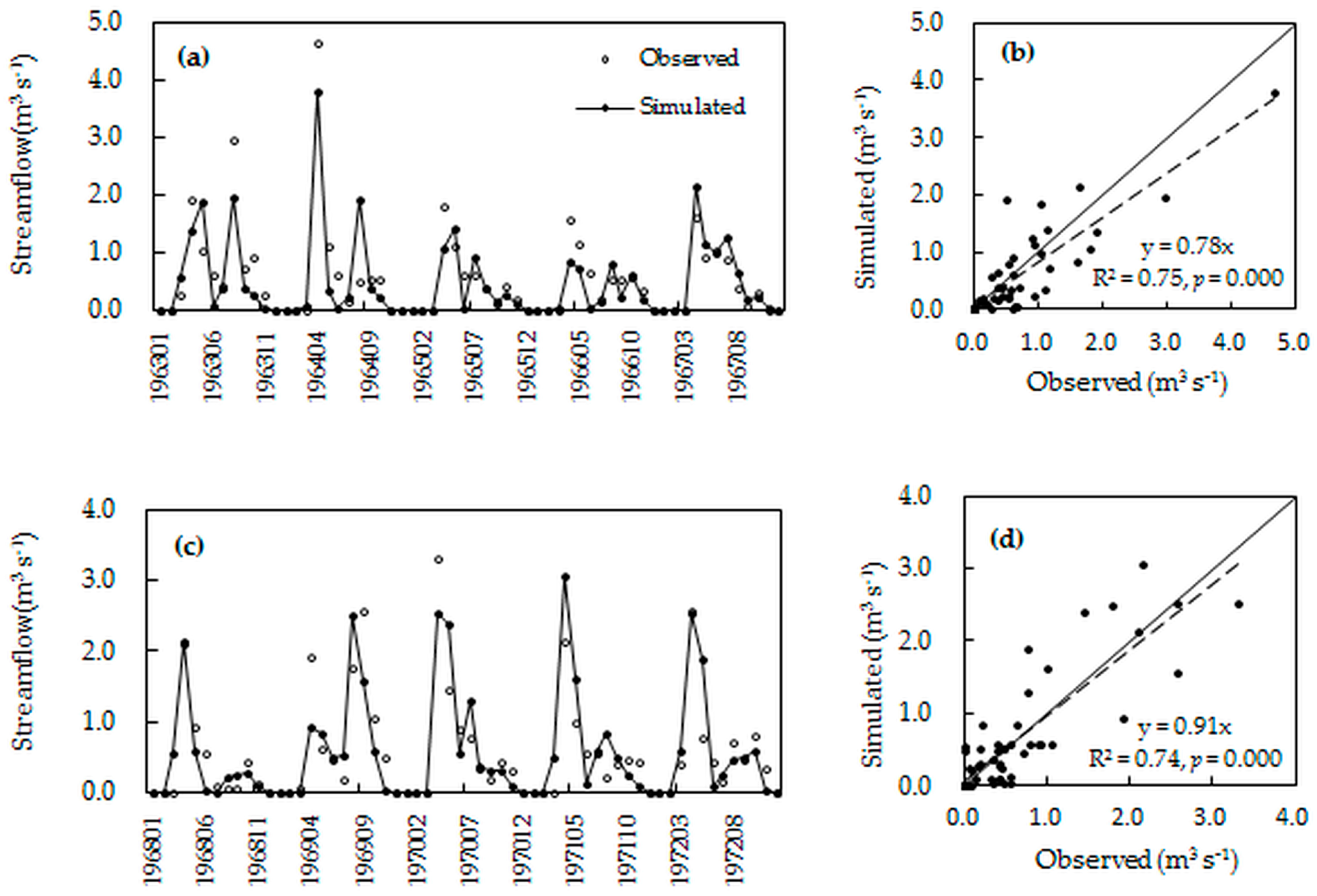
The vegetation cover changes due to climate change and human disturbances can change rangeland ecosystems considerably through altering the land use/cover patterns and ecosystem water balances between rainfall and ET [4,52]. Simulation method provides an effective and promising method that can support the understanding of dynamics, processes and the formation mechanism of environmental risk [53,54]. This study offers an improved SWAT model to simulate the response of streamflow to vegetation cover change and climate variations under multiple scenarios and aims to understand the ecohydrological responses of a water-limited environment to climate changes and to human activities. The results showed that the improved SWAT model simulations matched well to measured monthly streamflow for both calibration periods with determination coefficient R² = 0.75 and Nash–Sutcliffe E_NS = 0.67, as well as validation periods with R² = 0.74 and E_NS = 0.68.

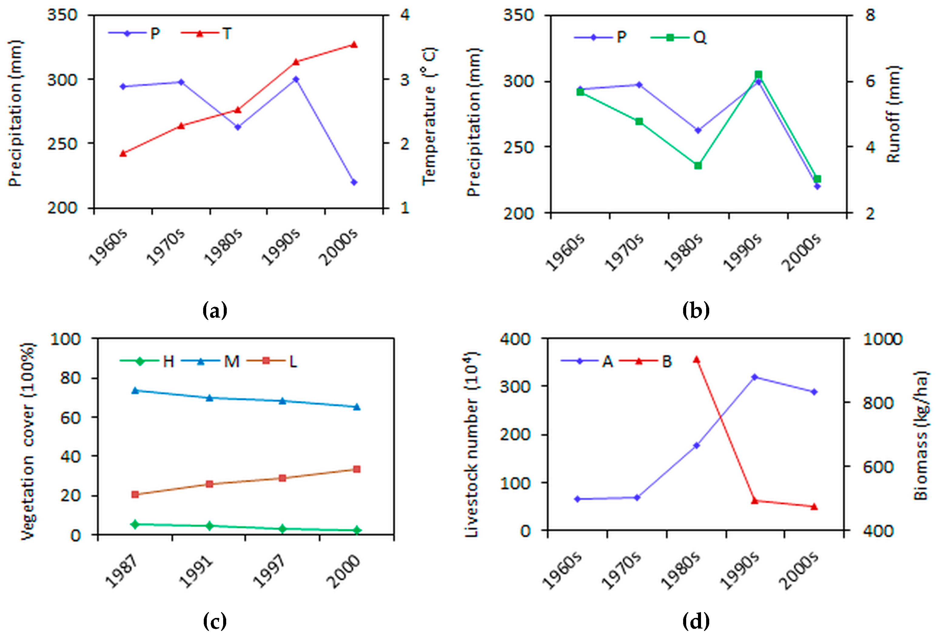
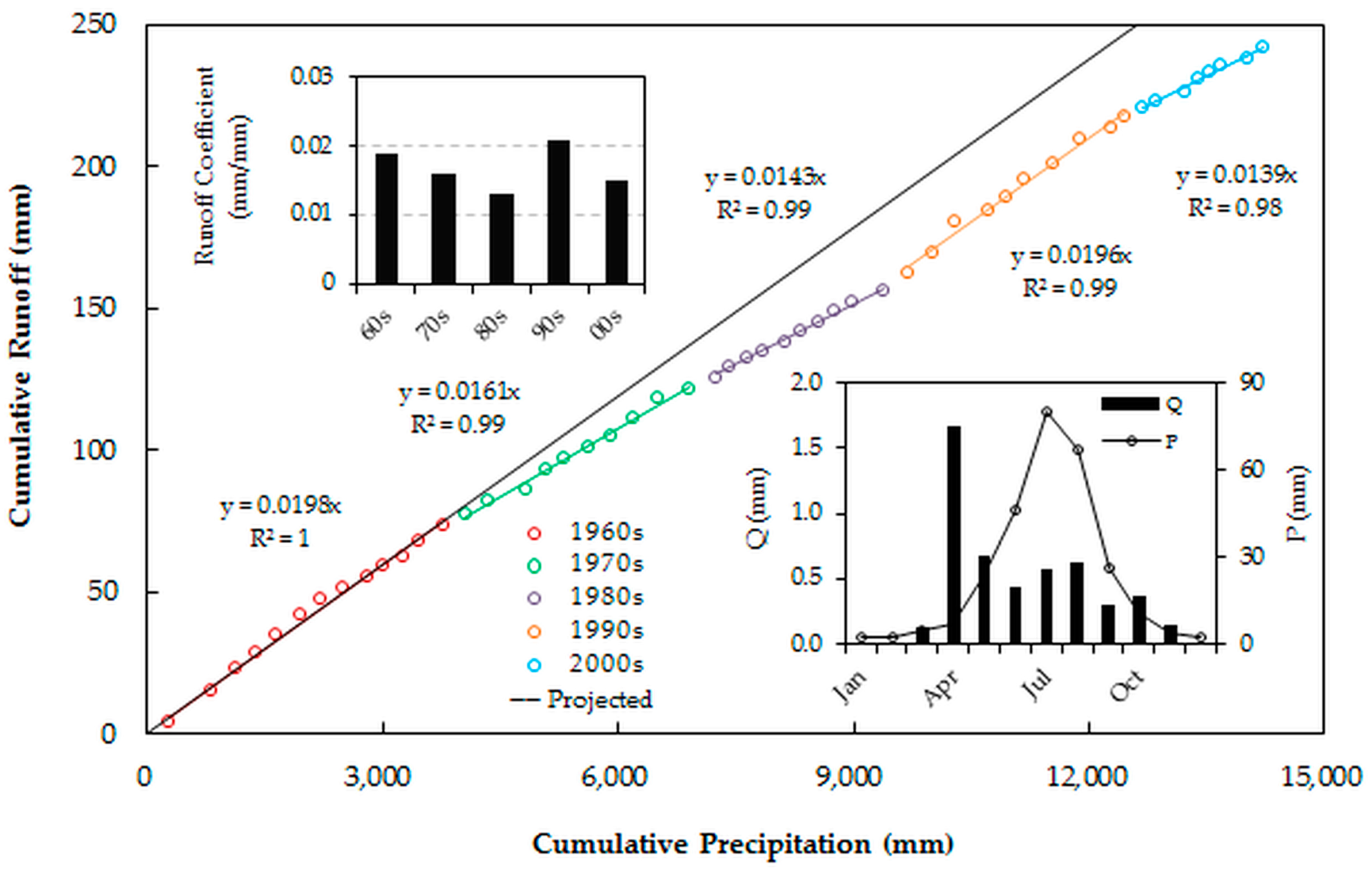
The simulating results indicated that precipitation dominated the water balances, and snow and permafrost melting in April dominated the annual river flow. The vegetation change scenario simulation results revealed that obvious changes occurred through conversion between high and low vegetation cover areas. The streamflow is sensitive to both climate variations and vegetation cover changes. The analysis suggests a clear association between streamflow change and precipitation variation, but also reveals that vegetation change may be an important factor. We also found the reductions in vegetation cover can elevate streamflow in both the rainfall season (July–August) and the snowmelt season (March–April), but the effects of the former are more obvious due to more vegetation cover in the rainfall season. These vegetation effects are more obvious during the periods with less rainfall or snowmelt. We conclude that in a particular climate zone, vegetation cover change is an important contributing factor to streamflow variations. Increases of streamflow in water-limited regions will likely reduce the effective water content of the soil, which in turn lead to further degradation of vegetation, particularly in the context of a drying and warming climate in this region.

Our study indicates that the ongoing large-scale degradation of vegetation due to overgrazing and other anthropogenic activities, such as mining and groundwater overuse, in the Xilin River Basin will likely change the hydrological environment and therefore increase the risk of ecological degradation and social vulnerability due to the loss of the ecosystem services of grassland vegetation. These findings highlight the importance of vegetation degradation on modifying the hydrological partitioning in the semi-arid steppe basin. The proposed relationship still needs to be evaluated in other catchments around the globe. The results contribute to the in-depth understanding of the mechanism of degradation and restoration of the grassland ecosystem and regional biophysical and physiological processes under global climate change, as well as provide critical information to develop methods and strategies towards sustainable development in the study basin and beyond.

References

1. Fraedrich, K.; Kleidon, A.; Lunkeit, F. A green planet versus a desert world: Estimating the effect of vegetation extremes on the atmosphere. J. Clim. 1999, 12, 3156–3163. [Google Scholar] [CrossRef]
2. Reynolds, J.F.; Stafford Smith, D.M.; Lambin, E.F.; Turner, B.L.; Mortimore, M.; Batterbury, S.P.; Downing, T.E.; Dowlatabadi, H.; Fernández, R.J.; Herrick, J.E.; et al. Global desertification: Building a science for dryland development. Science 2007, 316, 847–851. [Google Scholar] [CrossRef] [PubMed]
3. Liang, W.; Bai, D.; Wang, F.; Fu, B.; Yan, J.; Wang, S.; Yang, Y.; Long, D.; Feng, M. Quantifying the impacts of climate change and ecological restoration on streamflow changes based on a Budyko hydrological model in China’s Loess Plateau. Water Resour. Res. 2015, 51, 6500–6519. [Google Scholar] [CrossRef]
4. Hao, L.; Sun, G.; Liu, Y.; Zhou, G.; Wan, J.; Zhang, L.; Niu, J.; Sang, Y.; He, J. Evapotranspiration and soil moisture dynamics in a temperate grassland ecosystem in Inner Mongolia, China. Trans. ASABE 2016, 58. [Google Scholar] [CrossRef]
5. Li, H.; Zhang, Y.; Vaze, J.; Wang, B. Separating effects of vegetation change and climate variability using hydrological modelling and sensitivity-based approaches. J. Hydrol. 2012, 420–421, 403–418. [Google Scholar] [CrossRef]
6. Kashaigili, J.J.; Majaliwa, A.M. Implications of land use and land cover changes on hydrological regimes of the Malagarasi River, Tanzania. J. Agric. Sci. Appl. 2013, 2, 45–50. [Google Scholar]
7. Zhen, L.; Ochirbat, B.; Lv, Y.; Wei, Y.J.; Liu, X.L.; Chen, J.Q.; Yao, Z.J.; Li, F. Comparing patterns of ecosystem service consumption and perceptions of range management between ethnic herders in Inner Mongolia and Mongolia. Environ. Res. Lett. 2010, 5. [Google Scholar] [CrossRef]
8. Hao, L.; Sun, G.; Liu, Y.; Gao, Z.; He, J.; Shi, T.; Wu, B. Effects of precipitation on grassland ecosystem restoration under grazing exclusion in Inner Mongolia, China. Lands. Ecol. 2014, 29, 1657–1673. [Google Scholar] [CrossRef]
9. Gumindoga, W.; Rientjes, T.H.M.; Haile, A.T.; Dube, T. Predicting streamflow for land cover changes in the Upper Gilgel Abay River Basin, Ethiopia: A TOPMODEL based approach. Phys. Chem. Earth 2014, 76–78, 3–15. [Google Scholar] [CrossRef]
10. Miao, B.L.; Liang, C.Z.; Wang, W.; Wang, L.X.; Yun, W.L. Effects of vegetation on degradation surface runoff of typical steppe. J. Soil Water Conserv. 2008, 22, 10–14. (In Chinese) [Google Scholar]
11. Wang, Y.L.; Yun, W.L.; Miao, B.L.; Liang, C.Z.; Wang, W. The pattern and dynamics of surface runoff in the typical steppe of Inner Mongolia. Res. Soil Water Conserv. 2008, 15, 114–122. (In Chinese) [Google Scholar]
12. Li, S.; Liang, W.; Fu, B.; Lv, Y.; Fu, S.; Wang, S.; Su, H. Vegetation changes in recent large-scale ecological restoration projects and subsequent impact on water resources in China’s Loess Plateau. Sci. Total Environ. 2016, 569–570, 1032–1039. [Google Scholar] [CrossRef] [PubMed]
13. Zhang, S.; Yang, H.; Yang, D.; Jayawardena, A. Quantifying the effect of vegetation change on the regional water balance within the Budyko framework. Geophys. Res. Lett. 2015. [Google Scholar] [CrossRef]
14. Guo, Y.; Shen, Y. Quantifying water and energy budgets and the impacts of climatic and human factors in the Haihe River basin, China: 1.Model and validation. J. Hydrol. 2015, 528, 206–216. [Google Scholar] [CrossRef]
15. Yang, Y.T.; Long, D.; Guan, H.D.; Liang, W.; Simmons, C.T.; Batelaan, O. Comparison of three dual-source remote sensing evapotranspiration models during the MUSOEXE-12 campaign: Revisit of model physics. Water Resour. Res. 2015, 51, 3145–3165. [Google Scholar] [CrossRef]
16. Arnold, J.G.; Srinivasan, R.; Muttiah, R.S.; Williams, J.R. Large area hydrologic modeling and assessment, pt.1: Model Developmen. J. Am. Water Resour. Assoc. 1998, 34, 73–89. [Google Scholar] [CrossRef]
17. Strauch, M.; Volk, M. SWAT plant growth modification for improved modeling of perennial vegetation in the tropics. Ecol. Model. 2013, 269, 98–112. [Google Scholar] [CrossRef]
18. Song, Y.H.; Ma, J.H. SWAT-Aided research on hydrological responses to ecological restoration: A case study of the Nanhe River Basin in Huajialing of Longxi Loess Plateau. Acta Ecol. Sin. 2008, 28, 636–644. (In Chinese) [Google Scholar]
19. Bai, S.Y.; Wang, L.; Shi, J.Q.; Li, W. Runoff simulation for Kaidu river basin based on SWAT model. J. Arid Land Resour. Environ. 2013, 27, 79–84. (In Chinese) [Google Scholar] [CrossRef]
20. Kang, E.S.; Chen, R.S.; Zhang, Z.H.; Ji, X.B.; Jin, B.W. Some scientific problems facing researches on hydrological processes in an inland river basin. Adv. Earth Sci. 2007, 22, 940–953. (In Chinese) [Google Scholar]
21. Yan, Y.; Hu, Y.F.; Liu, Y.; Yu, G.M. The tendency and its spatial pattern of grassland changes in the East Xilin Gol from 1975 to 2009. J. Geo-Inf. Sci. 2011, 13, 549–555. [Google Scholar] [CrossRef]
22. Kawamura, K.; Akiyama, T.; Yokota, H.; Tsutsumi, M.; Yasuda, T.; Watanabe, O.; Wang, G.; Wang, S. Monitoring of forage conditions with MODIS imagery in the Xilingol steppe, Inner Mongolia. Int. J. Remote Sens. 2005, 26, 1423–1436. [Google Scholar] [CrossRef]
23. Chen, S.Q.; Liu, J.Y.; Zhuang, D.F.; Xiao, X.M. Quantifying land use and land cover change in Xilin River Basin using muti-temporal landsat TM/ETM sensor data. Acta Geogr. Sin. 2003, 58, 45–52. (In Chinese) [Google Scholar]
24. Liu, Y.; Zhou, Y.; Ju, W.; Chen, J.; Wang, S.; He, H.; Wang, H.; Guan, D.; Zhao, F.; Li, Y.; et al. Evapotranspiration and water yield over China’s landmass from 2000 to 2010. Hydrol. Earth Syst. Sci. 2013, 17, 4957–4980. [Google Scholar] [CrossRef]
25. Zhao, H.S. Studies on the ground water in the seasonal frozen soil region. Acta Pedol. Sin. 1981, 18, 389–394. (In Chinese) [Google Scholar]
26. Jiang, Y.; Bi, X.; Huang, J.; Bai, Y. Patterns and drivers of vegetation degradation in Xilin river basin, Inner Mongolia, China. J. Plant Ecol. 2010, 34, 1132–1141. (In Chinese) [Google Scholar]
27. The Office for the Second National Soil Survey of China (OSNSSC). Soil Series of China; Agricultural Press: Beijing, China, 1996; pp. 1–898. [Google Scholar]
28. Shi, X.Z.; Yu, D.S.; Warner, E.D.; Sun, W.X.; Petersen, G.W.; Gong, Z.T. Cross-reference system for translating between genetic soil classification of China and Soil Taxonomy. Soil Sci. Soc. Am. J. 2006, 70, 78–83. [Google Scholar] [CrossRef]
29. China Soil Database. Available online: http://gis.soil.csdb.cn/ (accessed on 14 August 2016).
30. Cai, Y.M.; Zhang, K.L.; Li, S.C. Study on the conversion of different soils texture. Acta Pedol. Sin. 2003, 40, 511–517. (In Chinese) [Google Scholar]
31. Saxton, K.E.; Rawls, W. Soil Water Characteristics Hydraulic Properties Calculator [EB/OL]. 2007. Available online: http://hydrolab.arsusda.gov/soilwater/Index.htm (accessed on 8 February 2017). [Google Scholar]
32. Nash, J.E.; Sutcliffe, J.V. River flow forecasting through conceptual models: Part 1—A discussion of principles. J. Hydrol. 1970, 10, 282–290. [Google Scholar] [CrossRef]
33. Sun, W.G.; Guo, X.Z.; Chen, X.X.; Sui, Y.; Qu, B.X. Analysis of semi-solidification effect and unconfined compressive strength of dredging spoil. Water Resour. Power 2012, 30, 41–43. (In Chinese) [Google Scholar]
34. Cheng, L.; Xu, Z.X.; Luo, R.; Mi, Y.J. SWAT application in arid and semi-arid region: A case study in the Kuye River Basin. Geogr. Res. 2009, 28, 65–73. (In Chinese) [Google Scholar]
35. Yang, D.; Shao, W.; Yeh, P.J.F.; Yang, H.; Kanae, S.; Oki, T. Impact of vegetation coverage on regional water balance in the nonhumid regions of China. Water Resour. Res. 2009, 45, W00A14. [Google Scholar] [CrossRef]
36. Boggs, J.L.; Sun, G. Urbanization alters watershed hydrology in the Piedmont of North Carolina. Ecohydrology 2011, 4, 256–264. [Google Scholar] [CrossRef]
37. Ludwig, J.A.; Wilcox, B.P.; Breshears, D.D.; Tongway, D.J.; Imeson, A.C. Vegetation patches and runoff–erosion as interacting ecohydrological processes in semiarid landscapes. Ecology 2005, 2, 288–297. [Google Scholar] [CrossRef]
38. Lei, H.; Yang, D.; Huang, M. Impacts of climate change and vegetation dynamics on runoff in the mountainous region of the Haihe River basin in the past five decades. J. Hydrol. 2014, 511, 786–799. [Google Scholar] [CrossRef]
39. Fuhlendorf, S.D.; Briske, D.D.; Smeins, F.E. Herbaceous vegetation change in variable rangeland environments: The relative contribution of grazing and climatic variability. Appl. Veg. Sci. 2001, 4, 177–188. [Google Scholar] [CrossRef]
40. Ash, A.J.; Corfield, J.P.; McIvor, J.G.; Ksiksi, T.S. Grazing Management in Tropical Savannas: Utilization and Rest Strategies to Manipulate Rangeland Condition. Rangel. Ecol. Manag. 2011, 64, 223–239. [Google Scholar] [CrossRef]
41. Golodets, C.; Kigel, J.; Sternberg, M. Recovery of plant species composition and ecosystem function after cessation of grazing in a Mediterranean grassland. Plant Soil 2010, 329, 365–378. [Google Scholar] [CrossRef]
42. Yeo, J.J. Effects of grazing exclusion on rangeland vegetation and soils, East Central Idaho. West. N. Am. Nat. 2005, 65, 91–102. [Google Scholar]
43. Zhang, X.S.; Tang, H.P.; Dong, X.B.; Li, B.; Huang, Y.M.; Gong, J.R. The dilemma of steppe and it’s transformation in China. Chin. Sci. Bull. 2016, 2, 165–177. [Google Scholar]
44. Qi, H.H.; Altinakar, M.S. A Conceptual Framework of Agricultural Land Use Planning with BMP for Integrated Watershed Management. J. Environ. Manag. 2011, 92, 149–155. [Google Scholar] [CrossRef] [PubMed]
45. Samaras, A.G.; Koutitas, C.G. The Impact of Watershed Management on Coastal Morphology: A Case Study Using an Integrated Approach and Numerical. Geomorphology 2014, 211, 52–63. [Google Scholar] [CrossRef]
46. Chomitz, K.M.; Kumari, K. The domestic benefits of tropical forests: A critical review. World Bank Res. Obs. 1998, 13, 13–35. [Google Scholar] [CrossRef]
47. Self-Davis, M.L.; Moore, P.A., Jr.; Daniel, T.C.; Nichols, D.J.; Sauer, T.J.; West, C.P.; Aiken, G.E.; Edwards, D.R. Forage species and canopy cover effects on runoff from small plots. J. Soil Water Conserv. 2003, 58, 349–359. [Google Scholar]
48. Huang, Y.L.; Fu, B.J.; Chen, L.D. Advances in ecohydrological process research. Acta Ecol. Sin. 2003, 23, 580–587. (In Chinese) [Google Scholar]
49. Sun, G.; McNulty, S.G.; Myers, J.A.M.; Cohen, E.C. Impacts of multiple stresses on water demand and supply across the southeastern United States. J. Am. Water Resour. Assoc. 2008, 44, 1441–1457. [Google Scholar] [CrossRef]
50. Zhang, L.; Podlasly, C.; Ren, Y.; Feger, K.H.; Wang, Y.; Schwärzel, K. Separating the effects of changes in land management and climatic conditions on long-term streamflow trends analyzed for a small catchment in the Loess Plateau region, NW China. Hydrol. Process 2014, 28, 1284–1293. [Google Scholar] [CrossRef]
51. Hao, L.; Sun, G.; Liu, Y.; Wan, J.; Qin, M.; Qian, H.; Liu, C.; Zheng, J.; John, R.; Fan, P.; et al. Urbanization dramatically altered the water balances of a paddy field-dominated basin in southern China. Hydrol. Earth Syst. Sci. 2015, 19, 3319–3331. [Google Scholar] [CrossRef]
52. Costa, M.H.; Botta, A.; Cardille, J.A. Effects of large-scale changes in land cover on the discharge of the Tocantins Rivers, Southeastern Amazonia. J. Hydrol. 2003, 283, 206–217. [Google Scholar] [CrossRef]
53. Gao, J.M. Analysis and assessment of the risk of Snow and Freezing Disaster in China. Int. J. Disast. Risk Reduct. 2016. [Google Scholar] [CrossRef]
54. Yu, H.; Wang, J.; Chai, M.; Shi, P.J. Review on research methods of disaster loss accumulation and amplification of disaster chains. Prog. Geogr. 2014, 11, 1498–1511. (In Chinese) [Google Scholar]
Figure 1. Location and land cover in the Xilin River Basin (2000).
Sustainability 09 00281 g001
Figure 2. DEM in the Xilin River Basin.
Sustainability 09 00281 g002
Figure 3. Soil type in the Xilin River Basin.
Sustainability 09 00281 g003
Figure 4. Mean annual precipitation (P) and (a) temperature (T); (b) the observed mean annual runoff (Q); (c) vegetation cover (H is high cover; M is moderate cover; and L is low cover; data source: [23]); and (d) livestock number (A, data source: Statistical Yearbook of Animal Husbandry in Inner Mongolia) and above ground biomass (B, data source: census data of grassland resources from Inner Mongolia Grassland Survey and Design Institute) in Xilin River Basin (1960s–2000s).
Sustainability 09 00281 g004
Figure 5. Double mass curve showing the relationships between accumulated annual precipitation (P) and total runoff (Q) for the Xilin River Basin (1958–2008). The left insert shows the runoff coefficient, the ratio of Q/P. The right insert shows the mean monthly Q and P.
Sustainability 09 00281 g005
Figure 6. Monthly time series comparison of observed versus simulated streamflow at the Xilin Reservoir Dam site using the improved SWAT model during (a,b) the calibration period (1963–1967) and (c,d) the validation period (1968–1972).
Sustainability 09 00281 g006
Figure 7. The livestock number change and management policies during the past decades in the XLRB (data source: Statistical Yearbook of Animal Husbandry in Inner Mongolia).
Sustainability 09 00281 g007
Figure 8. “Water-grass-livestock” conceptual framework for integrated watershed management in water-constrained pasture basins.
Sustainability 09 00281 g008