Article

Cloud Properties under Different Synoptic Circulations: Comparison of Radiosonde and Ground-Based Active Remote Sensing Measurements

1
Key Laboratory of Middle Atmosphere and Global Environment Observation, Institute of Atmospheric Physics, Chinese Academy of Sciences, Beijing 100029, China
2
Center of Technical Support and Service, Institute of Atmospheric Physics, Chinese Academy of Sciences, Beijing 100029, China
3
Collaborative Innovation Center on Forecast and Evaluation of Meteorological Disasters, Nanjing University of Information Science & Technology, Nanjing 210044, China
*
Author to whom correspondence should be addressed.
Atmosphere 2016, 7(12), 154; https://doi.org/10.3390/atmos7120154
Submission received: 30 August 2016 / Revised: 14 November 2016 / Accepted: 22 November 2016 / Published: 28 November 2016

Abstract

:
In this study, long-term (10 years) radiosonde-based cloud data are compared with the ground-based active remote sensing product under six prevailing large-scale synoptic patterns, i.e., cyclonic center (CC), weak pressure pattern (WP), the southeast bottom of cyclonic center (CB), cold front (CF), anticyclone edge (AE) and anticyclone center (AC) over the Southern Great Plains (SGP) site. The synoptic patterns are generated by applying the self-organizing map weather classification method to the daily National Centers for Environmental Protection mean sea level pressure records from the North American Regional Reanalysis. It reveals that the large-scale synoptic circulations can strongly influence the regional cloud formation, and thereby have impact on the consistency of cloud retrievals from the radiosonde and ground-based cloud product. The total cloud cover at the SGP site is characterized by the least in AC and the most in CF. The minimum and maximum differences between the two cloud methods are 10.3% for CC and 13.3% for WP. Compared to the synoptic patterns characterized by scattered cloudy and clear skies (AE and AC), the agreement of collocated cloud boundaries between the two cloud approaches tends to be better under the synoptic patterns dominated by overcast and cloudy skies (CC, WP and CB). The rainy and windy weather conditions in CF synoptic pattern influence the consistency of the two cloud retrieval methods associated with the limited capabilities inherent to the instruments. The cloud thickness distribution from the two cloud datasets compares favorably with each other in all synoptic patterns, with relative discrepancy of ≤0.3 km.

1. Introduction

Clouds have a critical influence on the Earth’s radiation budget and climate change [1]. Cloud vertical structures can interact with atmospheric dynamics and have a pronounced impact on the climate sensitivity [2,3,4]. Despite their significance, the accurate information of cloud profile is one of the most fundamental data sources for global weather and climate studies [5]. Thus far, significant discrepancies still exist in cloud retrievals from different cloud products [6,7,8].
To produce the reliable cloud climatology from various measurements at a regional scale, the U.S. Department of Energy’s Atmospheric Radiation Measurement (ARM) program has deployed a suite of ground-based remote sensing instruments at a few fixed sites. As the first ARM field measurement site, the Southern Great Plains (SGP) Central Facility site near Lamont, Oklahoma has been providing cloud data collected by the surface radar, ceilometers and lidar for over two decades. The cloud vertical structure information is available as an Active Remote Sensing of Cloud (ARSCL) value-added product (VAP) over the site [9]. The ARSCL has become a popular product in cloud research for numerous applications, for example, to obtain the regional cloud characteristics, to evaluate the satellite measurements and numerical models [10,11,12,13].
In addition to the ground-based instruments, the radiosonde launches have also been conducted for many years over the SGP site. By performing in-situ measurements of atmospheric temperature and humidity, the radiosonde is able to provide cloud information thus can be used to generate the cloud vertical structure [14,15,16,17,18,19]. To supply the measurements obtained from the ARM fix sites, an ARM mobile facility (AMF) was deployed in China in 2008 [20,21]. Zhang et al. [22] deployed the radiosonde data collected from this AMF campaign to analyze the cloud distributions over the site by using a modified method of [23] that employed the relative humidity (RH) and temperature profiles from the radiosonde data to determine the locations and boundaries of cloud layer. A preliminary validation of this method was further conducted based on the radiosonde data collected from different climate regimes, which suggested this method could produce a promising accuracy [24]. Costa-Surós et al. [25] summarized all the previous radiosonde-based cloud vertical structure estimation methods and also compared cloud vertical profiles to the ARSCL product at the SGP site. More importantly, they modified the method presented by [22] and their results demonstrated a better agreement between radiosounding method and ARSCL observations.
The local weather conditions and their changes are highly associated with the large-scale synoptic circulations. The atmospheric variables, such as temperature, RH, wind, and cloud distributions as well as their vertical structures can also be closely related to the large-scale synoptic circulations [26,27,28,29,30,31,32]. Therefore, the identification of large-scale synoptic patterns could be the basis on which to improve the understanding of the consistencies in cloud retrievals from various observational data as well as to determine the potential attributed sources of their differences. Based on this consideration, a comprehensive comparison of long-term (2001–2010) cloud products generated from the radiosonde and ground-based cloud retrieval approaches is performed at the SGP site on the basis of the classification of large-scale synoptic patterns in this study. It will help prompt knowledge of the interaction between the large-scale synoptic circulations and the regional cloud properties, and thereby quantitatively evaluate whether/how the synoptic patterns can influence the consistency and/or discrepancy between the cloud retrievals from the radiosonde and ARSCL data. Another important objective is to seek the potential causes for these differences. It is hoped that the results of this paper can assist with climate model performance by expanding our capability to derive cloud boundaries from the radiosonde to evaluate models over locations where ground-based radar and lidar are not deployed. The paper is organized as follows. Section 2 describes the two cloud detection algorithms and synoptic patterns data used in this study. Comparisons of cloud retrievals from two types of observational datasets are performed under different large-scale synoptic patterns in Section 3; potential causes for the discrepancies are also discussed. Main conclusions are summarized in Section 4.

2. Method and Data

2.1. Radiosonde-Based Cloud Detection Algorithm and Products

Radiosonde launches with a vertical resolution of ~10 m are generally conducted four times each day (at 05:30, 11:30, 17:30, and 23:30 UTC) over the SGP site. By using the algorithm presented in [24], radiosonde data collected over the SGP site between 2001 and 2010 were used to derive cloud layers in this study. A brief description of the algorithm is presented here while detailed procedure can be found in the above literature. The algorithm originates from the method of [23] with many modifications. It employs height-resolving RH thresholds to determine the cloud layers after transforming the RH with respect to ice for the levels with temperatures below 0 °C.

2.2. ARSCL Products

Three ground-based active remote sensors that are the 35-GHz Millimeter Microwave Cloud Radar (MMCR), Micropulse Lidar (MPL), and laser ceilometers have been deployed at the SGP site during the period of our study concerned [11,33,34,35,36,37]. The vertical resolutions of MMCR and MPL are 45- and 30-m respectively. A Vaisala CT25K ceilometer (15-m resolution), which can provide very accurate cloud base height up to ~7620 m, was deployed from May 2000 to April 2010. The CT25K ceilometer was then replaced with a Vaisala CL 31 to provide greater resolution (10-m). The MPL can detect cloud bases up to 18 km in the absence of any hazy layer and lower cloud layer. ARM cloud radars have a maximum detection range of ~20 km. The laser beams from the MPL and the ceilometers are excellent for detecting all clouds that are visible from the ground to the instruments’ height measurement ranges, but easily attenuated as they pass through cloud layers. The detection of cloud-base heights from radar is often affected by the presence of large precipitation particles, as well as insects and bits of vegetation. The radar is unable to detect some of clouds composed of small hydrometeors or thin clouds located at high altitudes. The greatest strength of radar measurements is to provide the cloud vertical distribution and to amend the drawback of lidar measurement, which cannot penetrate thick clouds. By combining the advantages of these three instruments, the ground-based cloud product (ARSCL) was generated by the ARM project [9,38]. This cloud product has a temporal resolution of 10 s and a vertical resolution of 45 m. A maximum of 10 cloud layers boundaries can be obtained from each ARSCL profile. The laser beams from the ceilometers and MPL are appropriate for providing first cloud base height. Hence, the Cloud Base Best Estimate (CBBE) field, which uses a mixture of ceilometer and MPL information, is deployed to filter hydrometeors below CBBE [39], which is specified as follows. The ARSCL cloud layers are discarded if both their cloud base heights and cloud top heights are lower than the CBBE. The cloud base height is set to CBBE for the ARSCL cloud layers with cloud base heights below the CBBE but the cloud top heights above the CBBE.

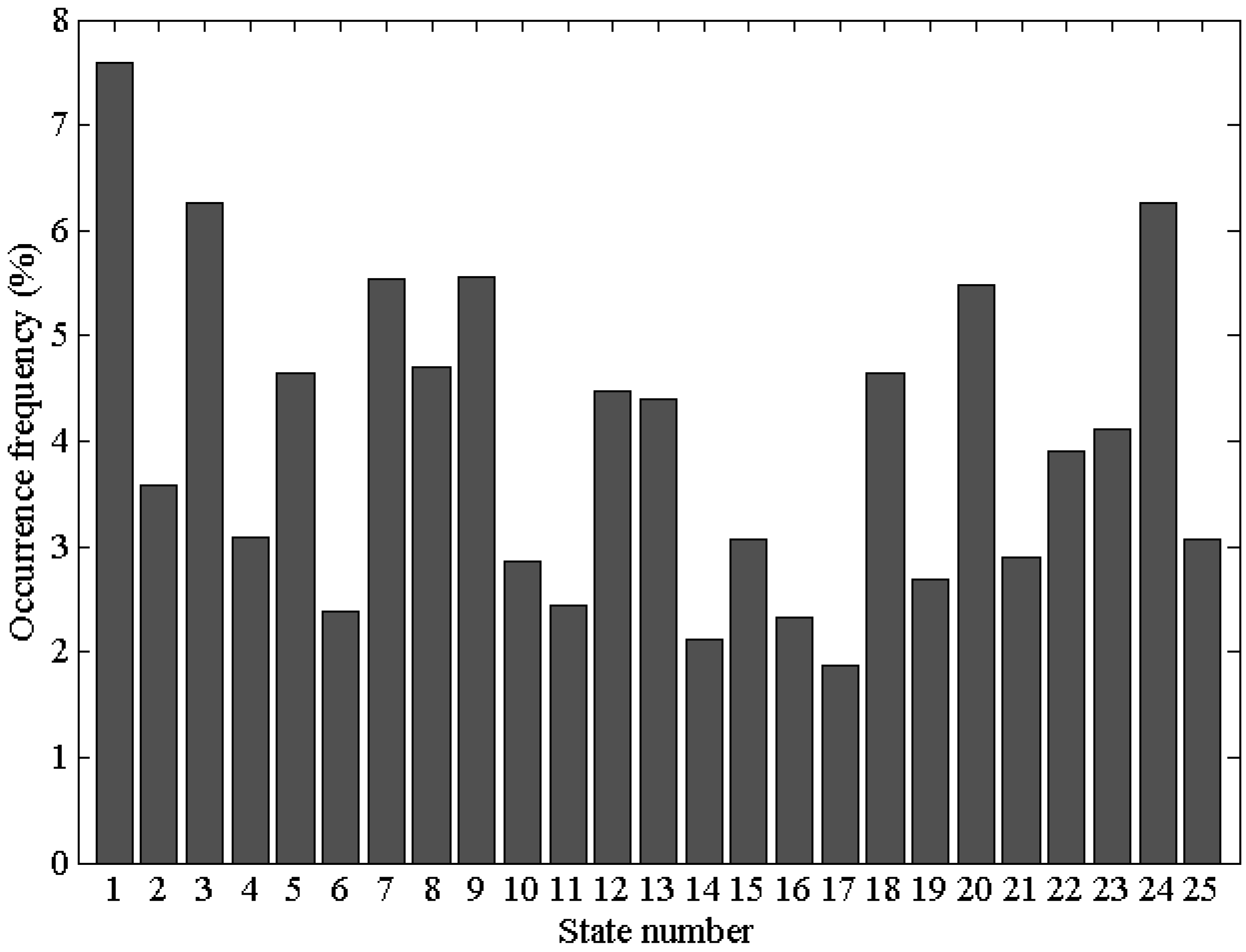
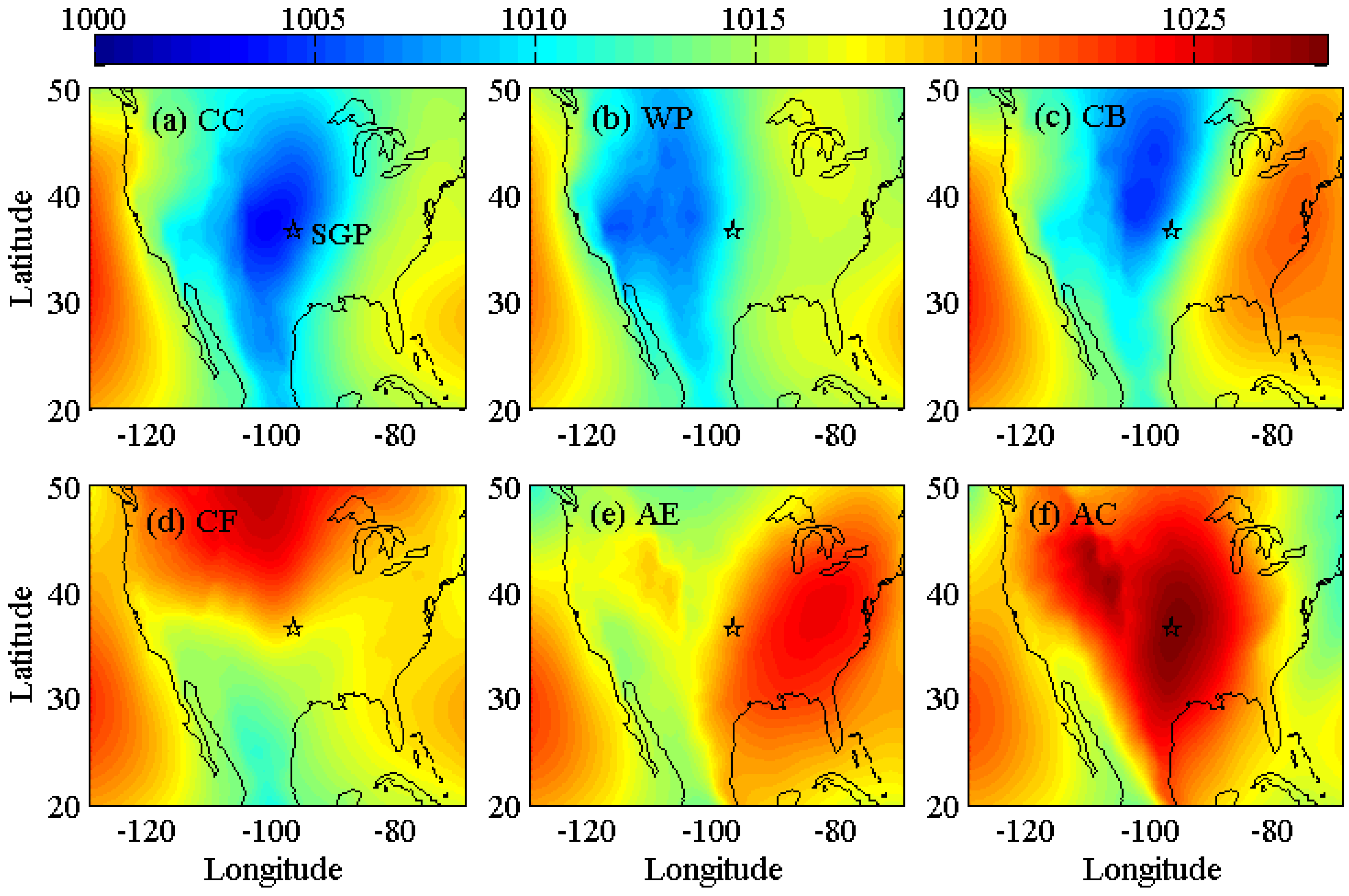
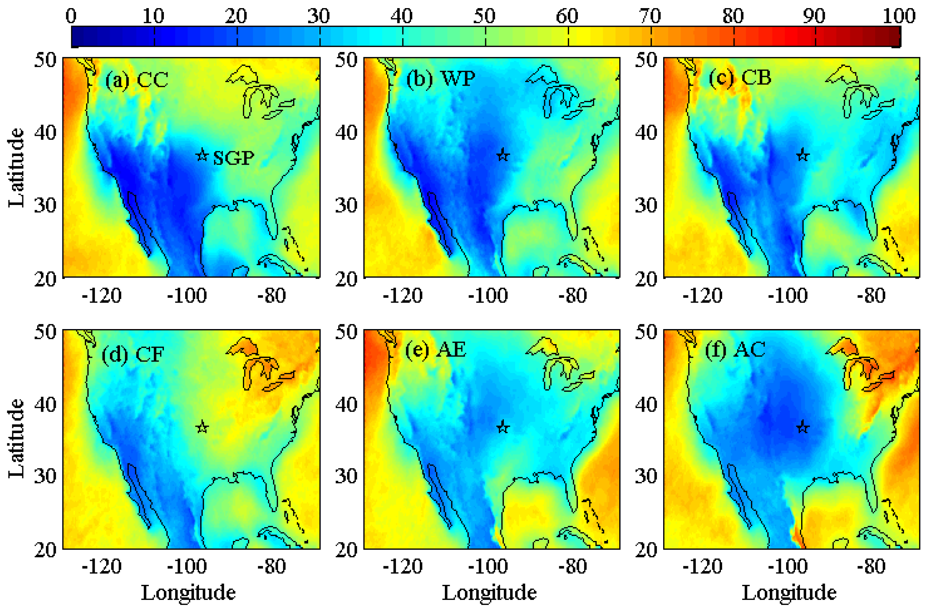
2.3. Synoptic Patterns Algorithm and Products

The synoptic patterns identification method used in this study is adopted from the approach of [40]. A detailed description of the weather classification can be found in the reference. A brief introduction is presented here for completeness. By applying the self-organizing map (SOM) method to 10 years of daily National Centers for Environmental Protection (NCEP) mean sea level pressure (MSLP) records from the North American Regional Reanalysis (NARR), a total of 25 synoptic patterns are characterized for the ARM SGP domain. The NCEP NARR products are used because they are the grid data with high spatial resolution (32 km × 32 km) and wide domain range (from 30°N to 50°N, and from 75°W to 120°W), which are specifically appropriate for the SOM method. The MSLP field associates highly with the spatial pattern of large-scale synoptic processes and is thus widely taken as a proxy for the atmospheric circulation [41]. As an artificial neural network algorithm used for clustering, visualization and abstraction, the SOM is very effective in studying the relationships between the local weather conditions and the large-scale climatology [42,43].
The occurrence frequencies of all 25 patterns at the SGP site are shown in Figure 1, with the maximum and minimum values of 7.6% and 1.9%, respectively. Six synoptic patterns are selected and discussed in this study. These 6 patterns are the cyclonic center (CC), the weak pressure pattern (WP), the southeast bottom of cyclonic center (CB), the cold front (CF), the anticyclone edge (AE) and the anticyclone center (AC), whose numbers are 1, 3, 5, 18, 20 and 24 in Figure 1, respectively. The typical patterns of CC, WP, AE and AC occurred most frequently, which account for 7.6%, 6.3%, 5.5% and 6.3%, respectively. The occurrence frequencies of both CB and CF are 4.7%. In the CB scenario, the weather conditions are dominated by cloudy skies associated with the moist southwesterly airflow at the 500-hPa level. In the CF scenario, drastic changes of synoptic patterns occur due to the intersection of cold and warm air masses. In view of the relative higher occurrence values compared to most of the other patterns as well as the typical synoptic features of CB and CF, they are also included in the study. The sum frequency of these selected 6 patterns is 35%. The percentage of situations represented by the other 19 patterns, which are discarded, is 65%. Some synoptic patters (e.g., 7 and 9) with large percentages of occurrence frequencies are discarded because they are the transition synoptic patters that are somewhat similar and relevant to the selected six patterns.
The MSLP, the geopotential height at the 500-hPa pressure level and the total cloud cover derived from the daily NCEP NARR product averaged over 2001–2010 under the selected six synoptic patterns are separately shown in Figure 2, Figure 3 and Figure 4. The geopotential heights at 500-hPa pressure level (not used by the SOM method) are deployed to help understand the air source of high altitude and background synoptic circulations of cloud formations. The major features of the six synoptic patterns and their general weather conditions are briefly introduced as follows. The SGP domain is located within the area of lowest atmospheric surface pressure in the CC pattern (Figure 2a); the skies are usually overcast due to the moist southwesterly airflow at the 500-hPa level over the SGP site (Figure 3a). In the WP scenario, the SGP site is within an area of weak depression at the surface; weather conditions are dominated by cloudy skies. In the CB scenario, the SGP site is located at the southeast bottom of a strong depression and near a strong anticyclone; conditions at the 500-hPa level are close to those in the CC pattern and weather conditions are dominated by cloudy skies. In the CF scenario, the SGP site is located in the transition zone between warm and cold air masses; the common weather conditions are rainy and windy under this synoptic pattern. In the AE scenario, the SGP site is situated at the rear of a strong anticyclone and the dominant airflow at the 500-hPa level is from the west; the weather conditions are usually clear or scattered cloudy sky. In the AC scenario, the SGP site is located in the center of anticyclone subsidence and is associated with strong divergence in the lower atmosphere; clear skies dominate as a result of the cold and dry northwest airflow at 500-hPa over the SGP site.

3. Comparison of Cloud Retrievals from Radiosonde and ARSCL in Different Synoptic Patterns

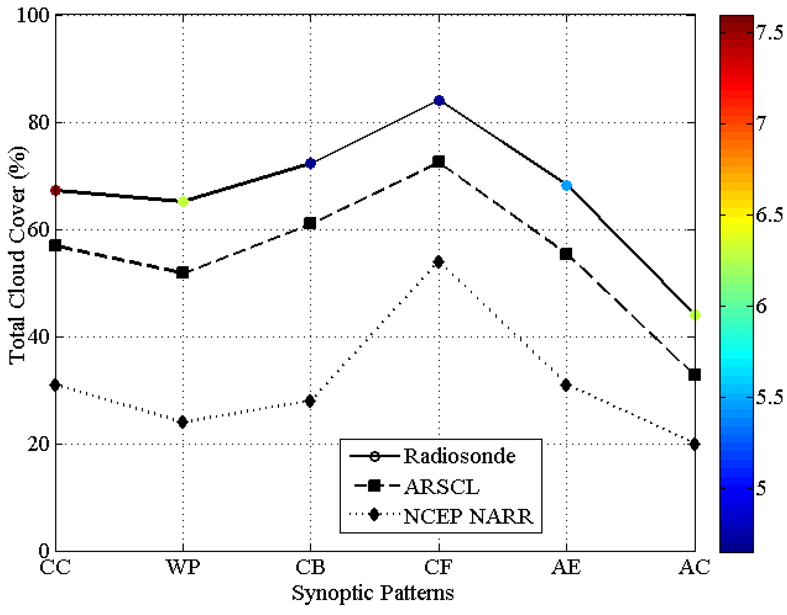
3.1. Total Cloud Cover

Ten years (2001–2010) of total cloud cover derived from the radiosonde and ARSCL products under six synoptic patterns are shown in Figure 5. The total cloud cover is defined as the number of samples with clouds present divided by the total number of ARSCL (or radiosonde) samples for each synoptic pattern. A total of 4575 radiosonde profiles are used in this study. The frequencies of cloud occurrence at the times of radiosonde launches are extremely likely different from that all day long obtained by the ground measurements due to the diurnal cycle of the cloud occurrence [44,45]. To avoid these potential diurnal cycle biases, the ARSCL data corresponding to the radiosonde launch periods are selected and used in this study. Colored dots (color bar) in Figure 5 represent the relative occurrence frequency (%) of each synoptic pattern during 2001–2010, varying from 4.7% (CB and CF) to 7.6% (CC). The NCEP NARR-based total cloud covers surrounding the SGP domain are also presented in Figure 5, which are 31%, 24%, 28%, 54%, 31% and 20% under six selected synoptic patterns, respectively, varying in a similar manner as that by the observational retrievals from both radiosonde and ground-based instruments. It is seen that the magnitude of the total cloud cover is highly dependent on the large-scale synoptic circulations. Both the radiosonde and ARSCL-based total cloud amounts over the SGP site are characterized by the least and the most occurred in patterns of AC (Radiosonde: 44%; ARSCL: 33%) and CF (Radiosonde: 84%; ARSCL: 72%), respectively. Overall, very similar manners of their variability are revealed by the two cloud measurements. However, a systematic difference occurs in the magnitude of total cloud cover between the two observational cloud products. Cloud amounts from the radiosonde measurements are always larger than the ARSCL products by ~10% for all six patterns. It should be noted that a similar systematic difference (8%) between radiosonde (59%: 114/193 cases) and ARSCL (51%: 99/193 cases) cloud retrieval methods was presented in [25] at the SGP site. In view of the high complexity and variations of the cloud distributions, the ARSCL product can express the total cloud cover well over the SGP site due to its high temporal resolution (ten seconds). The systematic difference between the two cloud products should be partially attributed to their different observation temporal intervals [4,11], and the mismatch of the objects detected by the two instruments due to the balloon’s drift and fixed ground-based observation [24]. The minimum and maximum differences between the two methods are 10.3% and 13.3% in patterns of CC and WP, respectively; their mean bias is 11.8% for all six patterns.

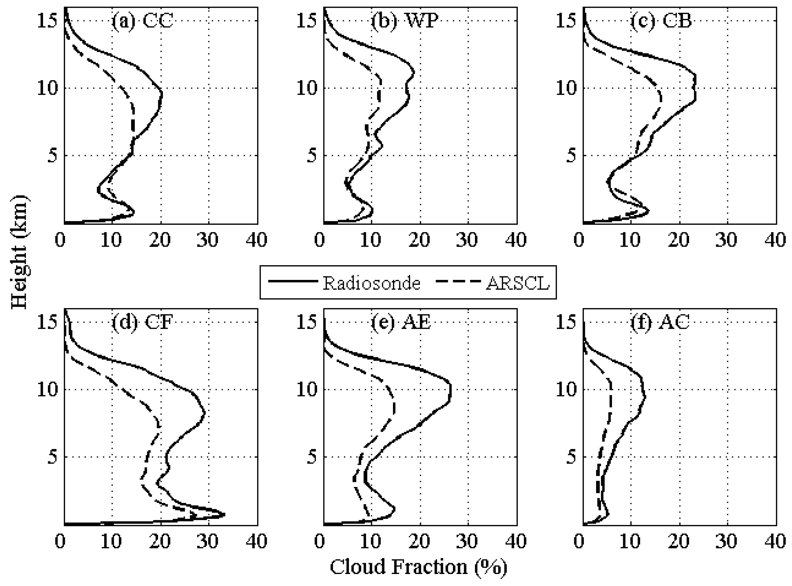
3.2. Vertical Cloud Fraction

Many years’ worth of radiosonde and ARSCL data at the SGP site allows for a closer look at the difference of the vertical cloud fraction between the two datasets at a fine vertical resolution, which should favor for the better understanding of their consistencies/discrepancies. The vertical resolutions of the radiosonde and ARSCL profiles are 10 m and 45 m, respectively. To make the comparison more meaningful, the vertical cloud fractions from both measurements are generated at atmospheric heights ranging from the surface to 16 km spaced at 100-m intervals (i.e., 0–100 m, 100–200 m, …, 15,900–16,000 m) and specified as follows. The radiosonde- and ground-based vertical cloud fractions in each 100-m bin is defined as the number of times a cloud or portion of cloud is detected in that bin divided by the total number of vertical profiles for each synoptic pattern. The average profiles of vertical cloud fractions derived from the two cloud products in six patterns during 2001–2010 are shown in Figure 6. A common characteristic exhibited by all six synoptic patterns is that the cloud retrievals from the two datasets are bimodal with a lower peak located in the boundary layer and an upper peak located in the high troposphere. However, large variations in magnitude are demonstrated among different synoptic patterns at a more detailed level. With regard to the lower-level peak, most cloud layers are detected in CF pattern (Radiosonde: 33%; ARSCL: 27%) and much fewer cloud layers occur in the other patterns, especially in AC (Radiosonde: 5%; ARSCL: 4%). For the upper-level peaks, the maximum and minimum values also occur in patterns of CF (Radiosonde: 29%; ARSCL: 20%) and AC (Radiosonde: 13%; ARSCL: 6%), respectively.
The agreement between the two cloud products is reasonable for the low/middle-level clouds located below 6 km at the majority of altitude levels in all six patterns. Their absolute difference is generally less than 3%, except that the relative larger bias of the two cloud approaches tends to occur in CF and AE patterns when the radiosonde overestimates the cloud fraction than the ARSCL estimation by at most up to ~5% at a few levels. Compared to the low/middle-level clouds, much greater discrepancies between the two methods are clearly demonstrated for the cloud layers in the upper troposphere. Many more high clouds are generated in all six patterns by the radiosonde than observed by the ARSCL products, which should be partially associated with the limitation of ground-based instruments in detecting some high cirrus associated with the attenuation effect of lower clouds and fog on the radar-lidar signals [7]. Furthermore, the magnitudes of the bias between the two cloud retrievals (radiosonde-ARSCL) vary among different synoptic patterns. Their maximum biases are 7.7%, 9.9%, 11.4%, 13.1%, 13.3% and 6.8% that generally locates at ~10 km for the six patterns, respectively. Although these biases are smallest in AC pattern (6.8%), it should be noted that its relative bias, denoted as (radiosonde-ARSCL)/radiosonde, is rather large because of the least clouds observed by the two approaches in this pattern.

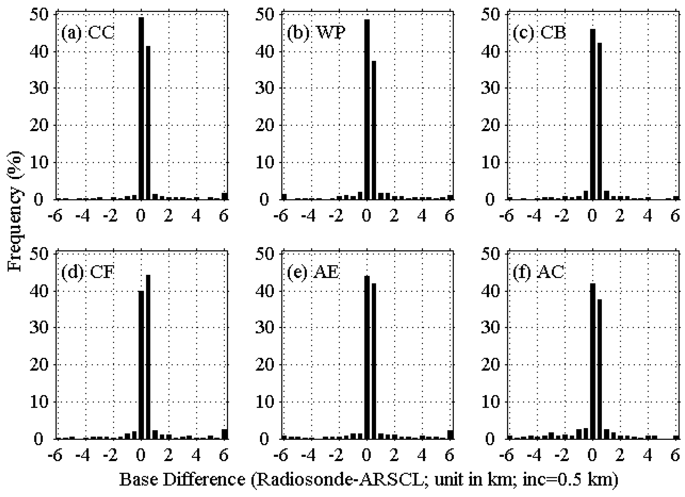
3.3. Collocation of Cloud Boundaries

The cloud boundaries, i.e., cloud-base height and cloud-top height derived from the radiosonde and ARSCL data, are compared according to different synoptic patterns in this section. The ground-based observations provide cloud information over the observational site, but the radiosonde measurements generate cloud information along a slanted pathway. When comparing the two cloud data sets, consideration must be taken of the differences caused by balloon drifting and the instantaneous nature of ground-based remote sensing measurements taken at a fixed site. Due to the cloud horizontal motion caused by the wind field, the ground-based data collected during a period of time could to some extent represent the cloud distributions over the areas surrounding the SGP site. To compensate the spatial difference between the radiosonde and ARSCL, comparisons of cloud boundaries cannot be limited to an instantaneous moment, but should be made for a certain time range. In this study, the cloud boundaries from ARSCL data collected during the radiosonde launch periods (generally 1.5 h for each radiosonde launch) are collocated in vertical with the radiosonde measurements. A total of 5278 collocated cloud boundaries from individual radiosonde and ARSCL retrievals are obtained from the six synoptic patterns. Figure 7 shows the comparisons of cloud-base heights between the two cloud retrieval methods. Colored dots in each panel represent the radiosonde drift distances when the cloud-base height is detected by the radiosonde. In general, a good agreement of the cloud-base heights between the radiosonde and ARSCL are demonstrated for all patterns, as shown by the vast majority of data points falling along or overlapping the 1:1 line. As indicated by the colors of the dots, a few outlier data are due in part to the mismatched observations in space between the radiosonde and ground-based measurements as a result of the relative large balloon drift distances [24]. The correlation coefficients are 0.93, 0.93, 0.95, 0.90, 0.90 and 0.90 for the six patterns. Given that most of data points are situated nearby the 1:1 line in Figure 7, the histograms of the differences for the cloud-base heights from the radiosonde and ARSCL data are further presented in Figure 8. The occurrence frequencies are ≥80% for the absolute differences of cloud base-heights less than 0.5 km in all six patterns, of which the maximum is 90% in CC pattern. The mean biases of the two retrievals (radiosonde-ARSCL) are 0.16 km, 0.26 km, 0.15 km and −0.14 km in CC, CF, AE and AC patterns, respectively; they are almost zero for both WP and CB patterns.
Figure 9 and Figure 10 show the comparison of collocated cloud-top heights retrieved from the two approaches under six patterns. Similar to the cloud-base heights, the agreements of the cloud-top heights are reasonable with most of the data points located in the vicinity of the 1:1 line; their correlation coefficients are generally larger than 0.90 with the maximum value of 0.95 in CB pattern. The mean biases (radiosonde-ARSCL) for cloud-top heights are 0.32 km, 0.16 km, 0.10 km, 0.47 km, 0.35 km and 0.01 km for the six patterns, respectively. The occurrence frequencies hover around 80% for their absolute differences of cloud top-heights less than 0.5 km under different synoptic patterns.
The previous comparisons of cloud-base height and cloud-top height are summarized in Table 1 and Table 2. Note that the clear sky cases are not taken into account in the standard deviation, correlation coefficient and the other parameters calculations. On average, both the cloud-base height and cloud-top height are generally higher in the radiosonde retrievals relative to the ARSCL measurements under different patterns. An exception occurs in AC pattern when lower cloud-base height is determined by the radiosonde relative to the ARSCL with a bias of −0.13 km. The few cloud layers in this pattern might increase the possibility of mismatch between radiosonde and ARSCL measurements as a result of the balloon drift. A much closer inspection of Table 1 and Table 2 further reveals a few interesting features. First, the correction coefficient (mean bias) generally varies in a similar trend for both cloud-base height and cloud-top height among the six patterns. This suggests that, for a certain synoptic pattern, it has the consistent impact on the agreement of the two methods in terms of both cloud-base height and cloud-top height. Second, the cloud boundaries tend to agree better for the two cloud methods in the synoptic patterns dominated by overcast and cloudy skies (CC, WP and CB) compared to the patterns characterized by scattered cloudy and clear skies (AE and AC). In the later synoptic categories, the occurrence and properties of scattered (or few) clouds are very complex and highly variable in space and time, which will influence the agreement of the two cloud methods due to the difference of the fixed ground-based instruments and drifting balloon. The maximum difference of the two cloud products occurs in CF pattern with an average bias of 0.26 (0.47) km for the cloud-base (cloud-top) height. The weather condition in this pattern is often rainy and windy. The performance of the radiosonde and ground-based cloud generations decreases under the rainy weather conditions due to the wetness of the radiosonde sensors and the attenuation effect of precipitation on the radar-lidar signals [7,24]; meanwhile, the wind will increase the radiosonde drift thus decrease the agreement of the two cloud products. Last, the agreement of the cloud-base height from the two approaches is better relative to the cloud-top retrievals, which can be explained as follows. Except that the attenuation effect of cloud layers deteriorates the capability of ground-based instruments in detecting the cloud-top height, the accuracy of radiosonde observations may become worse within a certain distance after the balloon travels through a cloud layer due to the time lag error associated with the wetness of the sensors [24]. However, it seems that this time lag effect may decrease in AC pattern which is dominated by clear sky and dry air in the atmosphere, resulting in a minimum bias of 0.01 km for the cloud-top height between the two estimations in this pattern (Table 2).

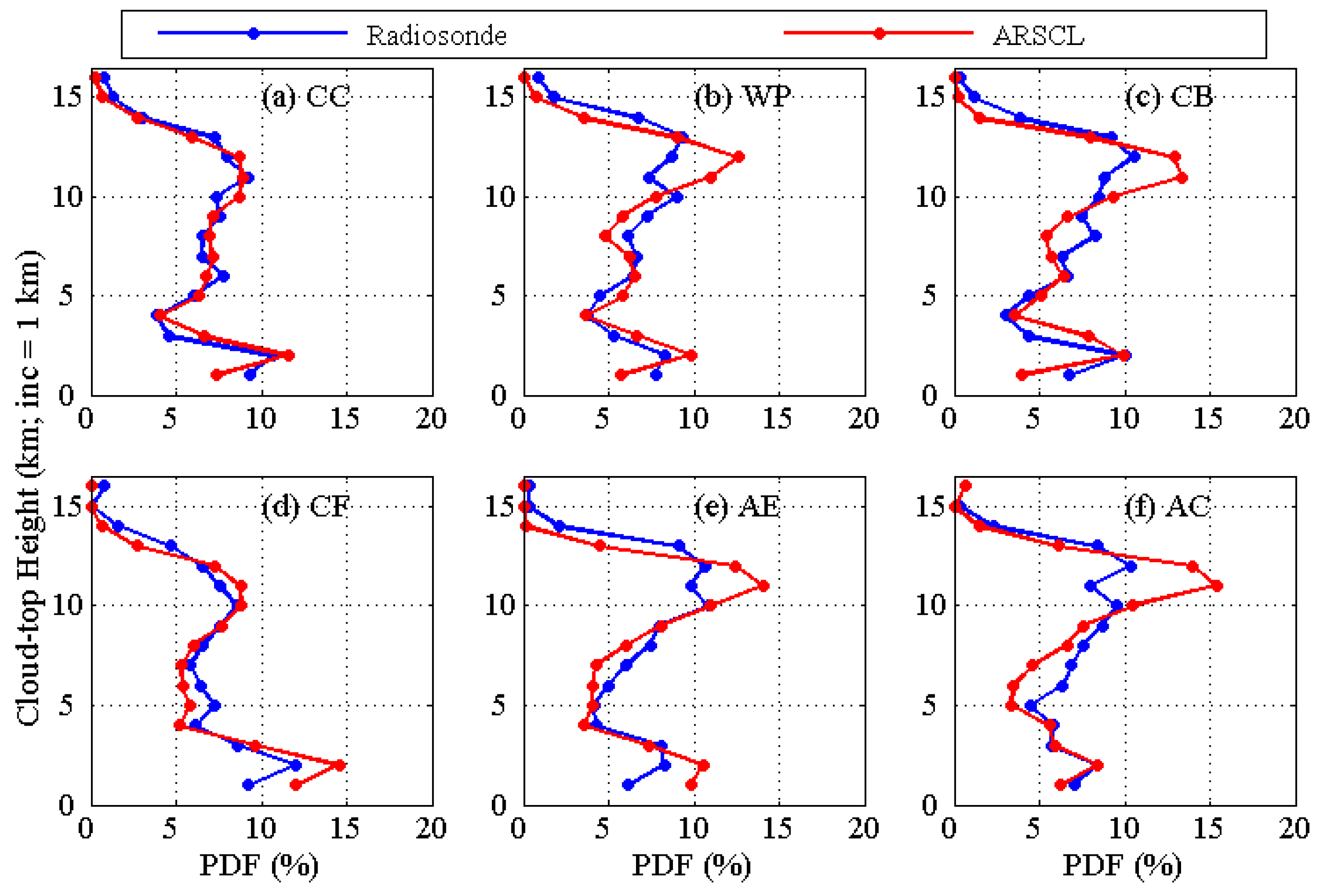
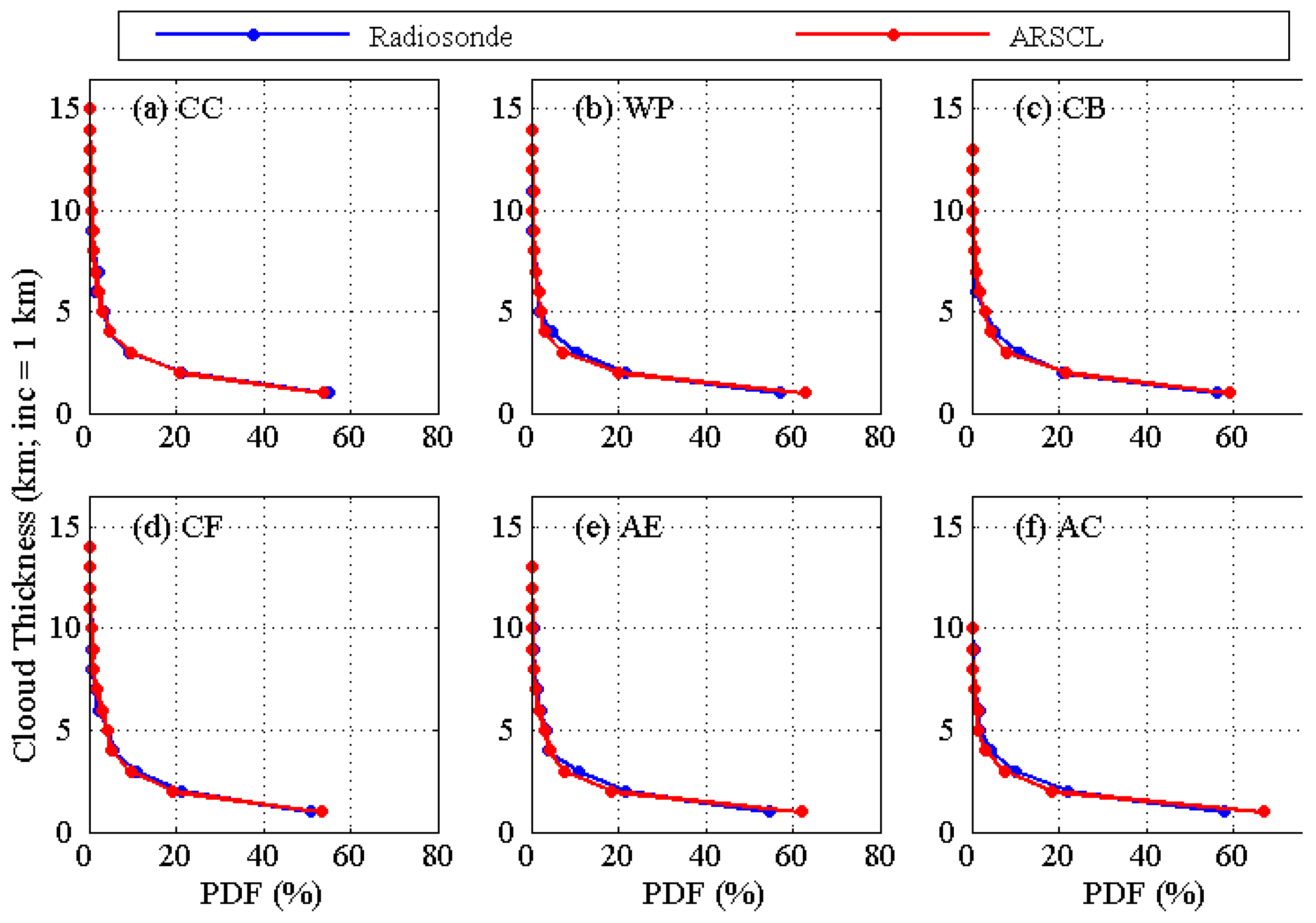
3.4. Vertical Distributions of Cloud-Base Height, Cloud-Top Height and Cloud Thickness

In view of fact that clouds in different vertical layers dictate the adiabatic heating rate and the radiation balance of the atmospheric column, the comparisons of the probability density functions (PDF) of the cloud-base height (CBH), cloud-top height (CTH) and cloud thickness (CT) of total cloud layers derived from the simultaneous radiosonde and ARSCL products collected during the radiosonde launch periods are further investigated in this section. Figure 11 presents the vertical PDFs of CBH spaced at 1 km interval for the six synoptic patterns. The two retrievals match fairly closely at all altitude levels in CC pattern which is frequently overcast. A uniform manner presented in the followed four patterns (WP, CB, CF and AE) is that the radiosonde-based PDF is often greater than the ARSCL measurements by <3% between 5 km and 10 km. Another distinct discrepancy should be noted is that the ARSCL-based PDF is greater than the radiosonde estimations by ~6% for CBH below 1 km in CF pattern. Although a similar structure is grossly presented by the two approaches in AC pattern, a displacement of the two profiles tends to occur in the vertical above 5 km; the ARSCL places the peak located around 11 km much higher in the upper troposphere relative to the radiosonde retrievals.
Figure 12 illustrates the vertical CTH PDF derived from the two methods under six synoptic patterns. Overall, radiosonde retrievals are very close to the ground-based remote sensing product in the CC pattern, being consistent with the CBH comparison conducted above. The two cloud approaches compare favorably with each other above 1 km in the CF pattern; however, the radiosonde differs greatly from ARSCL for CTH ≤ 1 km by 3%. Relative to the radiosonde, ARSCL data tend to overestimate the CTH PDF at 10–12 km in remaining four patterns; the maximum absolute difference is 7% at 11 km in AC pattern. The radiosounding method may miss some thin high cloud layers because the radiosonde may not detect changes in the relative humidity due to its decreasing performance at high altitude levels. However, less CTH PDF is generally reported by ARSCL at 5–10 km and above 12 km.
The occurrence frequencies of CT spaced at 1 km interval for six patterns are shown in Figure 13. In general, excellent agreements of CT distribution between the two cloud retrievals are exhibited in all patterns; the most PDF (~80%) occurs in CT ≤2 km. At a more detailed level, it is revealed that the greater PDF for CT ≤ 1 km tends to be detected by ARSCL than estimated by the radiosonde with the maximum difference of 9% in AC pattern. This is likely that the radiosonde miss some thin high cloud layers due to its decreasing performance of relative humidity detections at high altitude levels. The mean thicknesses derived from the radiosonde (ARSCL) cloud products are 1.5 (1.6) km, 1.3 (1.2) km, 1.4 (1.3) km, 1.7 (1.7) km, 1.5 (1.3) km and 1.3 (1.0) km for the six synoptic patterns, respectively. The thickest cloud layers are simultaneously detected by the two datasets in CF pattern (1.7 km). Overall, the mean thickness of the two cloud methods agrees well; their largest discrepancy is 0.3 km in AC pattern.

4. Conclusions

A profound knowledge of cloud profile is undoubtedly required for furthering our understanding of cloud climate effects. However, significant discrepancies still exist in cloud retrievals from different cloud products associated with their various inherent features and the high complexity of cloud distributions. Therefore, comparison of cloud profiles from different methods is of significance that is absolutely required for the improvement of these methods. As the major field measurement facility established by the Department of Energy’s ARM program in north-central Oklahoma, cloud product from the ground-based active remote sensing sensors has been provided at the SGP site over many years. Meanwhile, the cloud profile can also be derived from the radiosonde measurements over this region. The cloud retrievals from these two methods are quantitatively compared according to six prevailing large-scale synoptic patterns in this study.
A clear interaction between the large-scale synoptic pattern and the regional cloud cover is revealed over the SGP domain. Both the radiosonde and ARSCL-based total cloud amounts over the SGP site are characterized by the least and the most occurred in patterns of AC (Radiosonde: 44%; ARSCL: 33%) and CF (Radiosonde: 84%; ARSCL: 72%), respectively, which is consistent with the variation trend exhibited by the NCEP NARR product. Moreover, the large-scale synoptic patterns have impact on the consistency of cloud retrievals from the radiosonde and ground-based cloud product. The minimum and maximum differences of total cloud cover between the radiosonde and ARSCL data are 10.3% and 13.3% in patterns of CC and WP, respectively; their mean bias is 11.8% for all six patterns. Compared to the synoptic patterns characterized by scattered cloudy and clear skies (AE and AC), the collocated cloud boundaries (cloud-base height and cloud-top height) tend to agree better for the two cloud methods in the synoptic patterns dominated by overcast and cloudy skies (CC, WP and CB); the rainy and windy weather conditions in CF synoptic pattern influence the consistency of the two cloud retrieval approaches. This should be associated with the various detecting capabilities inherent to the two types of instruments, the difference between the fixed ground-based instruments and the drifting balloon, and the high complexity and variations of the cloud distributions. Excellent agreements of the cloud thickness between the two cloud retrievals are exhibited in all six patterns.
Validation of climate models requires an accurate knowledge of cloud macrophysical properties from the observational data. The current study provides the statistical characteristics of consistencies and/or discrepancies between the radiosonde- and surface-based cloud products on basis of six prevailing large-scale synoptic circulations. Several potential factors accounting for their discrepancies are also discussed. The results are expected to be beneficial for obtaining a more reliable cloud product to be used for the validation of climate model simulations.

Acknowledgments

The data from the U.S. Department of Energy’s Atmospheric Radiation Measurement (ARM) Climate Research Facility located near Lamont, Oklahoma were used in this study. This work was supported by the National Natural Science Foundation of China (No. 41175031, 41275039, 61327810, 91337214, and 41305011).

Author Contributions

The study was carried out in collaboration between all authors. Jinqiang Zhang wrote the manuscript; Xiangao Xia and Hongbin Chen revised the manuscript; and Jinqiang Zhang, Jun Li and Chao Ling analyzed the data. All authors agreed to the submission of the manuscript.

Conflicts of Interest

The authors declare no conflict of interest.

References

  1. Ramanathan, V.; Cess, R.D.; Harrison, E.F.; Minnis, P.; Barkstrom, B.R.; Ahmad, E.; Hartmann, D. Cloud-radiative forcing and climate: Results from the earth radiation budget experiment. Science 1989, 243, 57–63. [Google Scholar] [CrossRef] [PubMed]
  2. Kalesse, H.; Kollias, P. Climatology of high clouds dynamics using profiling ARM Doppler radar observations. J. Clim. 2013, 26, 6340–6359. [Google Scholar] [CrossRef]
  3. Sherwood, S.C.; Bony, S.; Dufresne, J.L. Spread in model climate sensitivity traced to atmospheric convective mixing. Nature 2014, 505, 37–42. [Google Scholar] [CrossRef] [PubMed]
  4. Zhang, J.; Chen, H.; Xia, X.; Wang, W.C. Dynamic and thermodynamic features of low and middle clouds derived from Atmospheric Radiation Measurement Program mobile facility radiosonde data at Shouxian, China. Adv. Atmos. Sci. 2016, 33, 21–33. [Google Scholar] [CrossRef]
  5. Stephens, G. Cloud feedbacks in the climate system: A critical review. J. Clim. 2005, 18, 237–273. [Google Scholar] [CrossRef]
  6. Thorsen, T.J.; Fu, Q.; Comstock, J.M.; Sivaraman, C.; Vaughan, M.A.; Winker, D.M.; Turner, D.D. Macrophysical properties of tropical cirrus clouds from the CALIPSO satellite and from ground-based micropulse and Raman lidars. J. Geophys. Res. 2013, 118, 9209–9220. [Google Scholar] [CrossRef]
  7. Protat, A.; Young, S.A.; McFarlane, S.; L’Ecuyer, T.; Mace, G.G.; Comstock, J.; Long, J.C.; Berry, E.; Delanoë, J. Reconciling ground-based and space-based estimates of the frequency of occurrence and radiative effect of clouds around Darwin, Australia. J. Appl. Meteor. Clim. 2014, 53, 456–478. [Google Scholar] [CrossRef]
  8. Dolinar, E.; Dong, X.; Xi, B.; Jiang, J.H.; Sui, H. Evaluation of CMIP5 simulated clouds and TOA radiation budgets using NASA satellite observations. Clim. Dyn. 2015, 44, 229–2247. [Google Scholar] [CrossRef]
  9. Clothiaux, E.E.; Ackerman, T.P.; Mace, G.G.; Moran, K.P.; Marchand, R.T.; Miller, M.A.; Martner, B.E. Objective determination of cloud heights and radar reflectivities using a combination of active remote sensors at the ARM CART sites. J. App. Meteorol. 2000, 39, 645–665. [Google Scholar] [CrossRef]
  10. Kollias, P.; Tselioudis, G.; Albrecht, B.A. Cloud climatology at the Southern Great Plains and the layer structure, drizzle, and atmospheric modes of continental stratus. J. Geophys. Res. 2007, 112. [Google Scholar] [CrossRef]
  11. Xi, B.; Dong, X.; Minnis, P.; Khaiyer, M.M. A 10 year climatology of cloud fraction and vertical distribution derived from both surface and GOES observations over the DOE ARM SGP Site. J. Geophys. Res. 2010, 115. [Google Scholar] [CrossRef]
  12. Qian, Y.; Long, C.N.; Wang, H.; Comstock, J.M.; McFarlane, S.A.; Xie, S. Evaluation of cloud fraction and its radiative effect simulated by IPCC AR4 global models against ARM surface observations. Atmos. Chem. Phys. 2012, 12. [Google Scholar] [CrossRef]
  13. Yoo, H.; Li, Z.; Hou, Y.; Lord, S.; Weng, F.; Barker, H. Diagnosis and testing of low-level cloud parameterizations for the NCEP/GFS model satellite and ground-based measurements. Clim. Dyn. 2013, 41, 1595–1613. [Google Scholar] [CrossRef]
  14. Chernykh, I.V.; Eskridge, R.E. Determination of cloud amount and level from radiosonde soundings. J. App. Meteorol. 1996, 35, 1362–1369. [Google Scholar] [CrossRef]
  15. Wang, J.; Rossow, W.B.; Uttal, T.; Rozendaal, M. Variability of cloud vertical structure during ASTEX observed from a combination of rawinsonde, radar, ceilometer, and satellite. Mon. Weather Rev. 1999, 127, 2482–2502. [Google Scholar] [CrossRef]
  16. Wang, J.; Rossow, W.B.; Zhang, Y. Cloud vertical structure and its variations from a 20-year global rawinsonde dataset. J. Clim. 2000, 13, 3041–3056. [Google Scholar] [CrossRef]
  17. Chernykh, I.V.; Alduchov, O.A.; Eskridge, R.E. Trends in low and high cloud boundaries and errors in height determination of cloud boundaries. Bull. Am. Meteorol. Soc. 2000, 82, 1941–1947. [Google Scholar] [CrossRef]
  18. Naud, C.; Muller, J.P.; Clothiaux, E.E. Comparison between active sensor and radiosonde cloud boundaries over the ARM Southern Great Plains site. J. Geophys. Res. 2003, 108. [Google Scholar] [CrossRef]
  19. Minnis, P.; Yi, Y.; Huang, J.; Ayers, J. Relationships between radiosonde and RUC-2 meteorological conditions and cloud occurrence determined from ARM data. J. Geophys. Res. 2005, 110. [Google Scholar] [CrossRef]
  20. Fan, X.; Chen, H.; Xia, X.; Li, Z.; Cribb, M. Aerosol optical properties from the Atmospheric Radiation Measurement Mobile Facility at Shouxian, China. J. Geophys. Res. 2010, 115. [Google Scholar] [CrossRef]
  21. Li, Z.; Li, C.; Chen, H.; Tsay, S.C.; Holben, B.N.; Huang, J.; Li, B.; Maring, H.; Qian, Y.; Shi, G.; et al. East Asian studies of tropospheric aerosols and their impact on regional climate (EAST-AIRC): An overview. J. Geophys. Res. 2011, 116. [Google Scholar] [CrossRef]
  22. Zhang, J.; Chen, H.; Li, Z.; Fan, X.; Peng, L.; Yu, Y.; Cribb, M. Analysis of cloud layer structure in Shouxian, China using RS92 radiosonde aided by 95 GHz cloud radar. J. Geophys. Res. 2010, 115. [Google Scholar] [CrossRef]
  23. Wang, J.; Rossow, W.B. Determination of cloud vertical structure from upper air observations. J. Appl. Meteorol. 1995, 34, 2243–2258. [Google Scholar] [CrossRef]
  24. Zhang, J.; Li, Z.; Chen, H.; Cribb, M. Validation of a radiosonde-based cloud layer detection method against a ground-based remote sensing method at multiple ARM sites. J. Geophys. Res. 2013, 118, 846–858. [Google Scholar] [CrossRef]
  25. Costa-Surós, M.; Calbó, J.; González, J.A.; Long, C.N. Comparing the cloud vertical structure derived from several methods based on radiosonde profiles and ground-based remote sensing measurements. Atmos. Meas. Techol. 2014, 7, 2757–2773. [Google Scholar] [CrossRef] [Green Version]
  26. Gordon, N.D.; Norris, J.R.; Weaver, C.P.; Klein, S.A. Cluster analysis of cloud regimes and characteristic dynamics of midlatitude synoptic systems in observations and a model. J. Geophys. Res. 2005, 110. [Google Scholar] [CrossRef]
  27. Marchand, R.; Beagley, N.; Thompson, S.; Ackerman, T.; Schultz, D. A bootstrap technique for testing the relationship between local-scale radar observations of cloud occurrence and large-scale atmospheric fields. J. Atmos. Sci. 2006, 63, 2813–2830. [Google Scholar] [CrossRef]
  28. Marchand, R.; Beagley, N.; Ackerman, T. Evaluation of hydrometeor occurrence profiles in the Multiscale Modeling Framework climate model using atmospheric classification. J. Clim. 2009, 22, 4557–4573. [Google Scholar] [CrossRef]
  29. Bailey, A.; Chase, T.N.; Cassano, J.J.; Noone, D. Changing temperature inversion characteristics in the U.S. Southwest and relationships to large-scale atmospheric circulation. J. Appl. Meteorol. Climatol. 2011, 50, 1307–1323. [Google Scholar] [CrossRef]
  30. Evans, S.M.; Marchand, R.T.; Ackerman, T.P.; Beagley, N. Identification and analysis of atmospheric states and associated cloud properties for Darwin, Australia. J. Geophys. Res. 2012, 117. [Google Scholar] [CrossRef]
  31. Scott, R.C.; Lubin, D. Mixed-phase cloud radiative properties over Ross Island, Antarctica: The influence of various synoptic-scale atmospheric circulation regimes. J. Geophys. Res. 2014, 119, 6702–6723. [Google Scholar] [CrossRef]
  32. Kennedy, A.; Dong, X.; Xi, B. Cloud Fraction at the ARM SGP Site. Reducing uncertainty with Self Organizing Maps. Theor. Appl. Climatol. 2015, 124, 43–54. [Google Scholar] [CrossRef] [PubMed]
  33. Moran, K.P.; Martner, B.E.; Post, M.J.; Kropfli, R.A.; Welsh, D.C.; Widener, K.B. An unattended cloud-profiling radar for use in climate research. Bull. Am. Meteorol. Soc. 1998, 79, 443–455. [Google Scholar] [CrossRef]
  34. Clothiaux, E.E.; Moran, K.P.; Martner, B.E.; Ackerman, T.P.; Mace, G.G.; Uttal, T.; Mather, J.H.; Widener, K.B.; Miller, M.A.; Rodriguez, D.J. The Atmospheric Radiation Measurement Program cloud radars: Operational modes. J. Atmos. Ocean. Technol. 1999, 16, 819–827. [Google Scholar] [CrossRef]
  35. Clothiaux, E.E.; Mace, G.G.; Ackerman, T.P.; Kane, T.J.; Spinhirne, J.; Scott, V.S. An automated algorithm for detection of hydrometeor returns in mico pulse lidar data. J. Atmos. Ocean. Technol. 1998, 15, 1035–1042. [Google Scholar] [CrossRef]
  36. Dupont, J.C.; Haefflein, M.; Morille, Y.; Comstock, J.M.; Flynn, C.; Long, C.N.; Sivaraman, C.; Newson, R.K. Cloud properties derived from two lidars over the ARM SGP site. Geophys. Res. Lett. 2011, 38. [Google Scholar] [CrossRef] [Green Version]
  37. Hogan, R.J.; Francis, P.N.; Flentje, H.; Illingworth, A.J.; Quante, M.; Pelon, J. Characteristics of mixed-phase clouds. I: Lidar, radar and aircraft observations from CLARE’98. Q. J. R. Meteorol. Soc. 2003, 129, 2089–2116. [Google Scholar] [CrossRef]
  38. Clothiaux, E.E.; Miller, M.A.; Perez, R.C.; Turner, D.D.; Moran, K.P.; Martner, B.E.; Ackerman, T.P.; Widener, K.B.; Rodriguez, D.J.; Uttal, T.; et al. The ARM Millimeter Wave Cloud Radars (MMCRs) and the Active Remote Sensing of Clouds (ARSCL) Value Added Product (VAP). DOE Tech. Memo. ARM VAP-002.1; U.S. Department of Energy: Washington, DC, USA, 2001. Available online: http://web.gps.caltech.edu/~drf/thumb/df_papers/clothiaux_2001_mmcr_arscl.pdf (accessed on 20 March 2016). [Google Scholar]
  39. Kennedy, A.; Dong, X.; Xi, B. Cloud fraction at the ARM SGP site Instrument and sampling considerations from 14 years of ARSCL. Theor. Appl. Climatol. 2014, 115, 91–105. [Google Scholar] [CrossRef]
  40. Li, J.; Chen, H.B.; Li, Z.Q.; Wang, C.P.; Cribb, M.; Fan, X.H. Low-level temperature inversions and their effect on aerosol condensation nuclei concentrations under different large-scale synoptic circulations. Adv. Atmos. Sci. 2015, 32, 898–908. [Google Scholar] [CrossRef]
  41. Huth, R.; Beck, C.; Philipp, A.; Demuzere, M.; Ustrnul, Z.; Cahynov, M.; Kysely, J.; Tveito, O.E. Classifications of atmospheric circulation patterns recent advances and applications. In Trends and Directions in Climate Research; Gimeno, L., Garcia-Herrera, R., Trigo, R.M., Eds.; Blackwell Publishing: Oxford, UK, 2008; pp. 105–152. [Google Scholar]
  42. Kohonen, T. The self-organizing map. Neurocomputing 1998, 21, 1–6. [Google Scholar] [CrossRef]
  43. Hewitson, B.C.; Crane, R.G. Self-organizing maps: Applications to synoptic climatology. Clim. Res. 2002, 22, 13–26. [Google Scholar] [CrossRef]
  44. Dong, X.; Xi, B.; Minnis, P. A climatology of mid-latitude continental clouds from the ARM SGP central facility. Part II: Cloud fraction and surface radiative forcing. J. Clim. 2006, 19, 1765–1783. [Google Scholar] [CrossRef]
  45. Zhang, Y.; Klein, S.A. Mechanisms affecting the transition from shallow to deep convection over land: Inferences from observations of the diurnal cycle collected at the ARM Southern Great Plains site. J. Atmos. Sci. 2010, 67, 2943–2959. [Google Scholar] [CrossRef]
Figure 1. Occurrence frequencies of 25 patterns during 2001–2010 at the SGP site.
Atmosphere 07 00154 g001
Figure 2. Mean sea level pressure (units in hPa) derived from the daily National Centers for Environmental Protection (NCEP), North American Regional Reanalysis (NARR) product averaged over 2001 to 2010 in the synoptic patterns of: cyclonic center: CC (a); weak pressure pattern: WP (b); the southeast bottom of cyclonic center: CB (c); cold front: CF (d); anticyclone edge: AE (e); and anticyclone center: AC (f) over the Southern Great Plains (SGP) site. The black star in each panel denotes the location of the SGP site.
Atmosphere 07 00154 g002
Figure 3. Geopotential height (units in m) at the 500-hPa pressure level derived from the daily NCEP NARR product averaged over 2001 to 2010 in the synoptic patterns of: CC (a); WP (b); CB (c); CF (d); AE (e); and AC (f) over the SGP site. The black star in each panel denotes the location of the SGP site.
Atmosphere 07 00154 g003
Figure 4. Total cloud cover (%) derived from the daily NCEP NARR product averaged over 2001 to 2010 in the synoptic patterns of: CC (a); WP (b); CB (c); CF (d); AE (e); and AC (f) over the SGP site. The black star in each panel denotes the location of the SGP site.
Atmosphere 07 00154 g004
Figure 5. Total cloud cover derived from the radiosonde data (solid line), ARSCL product (long dashed line), and NCEP NARR (short dashed line) for the six synoptic patterns (CC, WP, CB, CF, AE and AC) during 2001–2010 at the SGP site. The color of the dots in radiosonde data represents the relative occurrence frequency (%) of each synoptic pattern during the period analyzed.
Atmosphere 07 00154 g005
Figure 6. Average profiles of vertical cloud fraction derived from the radiosonde data (solid line) and ARSCL product (dashed line) for the synoptic patterns of: CC (a); WP (b); CB (c); CF (d); AE (e); and AC (f) during 2001–2010 at the SGP site. The vertical resolution is 100 m.
Atmosphere 07 00154 g006
Figure 7. Comparison of collocated cloud-base heights derived from the radiosonde and ARSCL data in the synoptic patterns of: CC (a); WP (b); CB (c); CF (d); AE (e); and AC (f) during 2001–2010 at the SGP site. Colored dots in each panel represent different radiosonde drift distances (DD; units in km).
Atmosphere 07 00154 g007
Figure 8. Histogram of difference of collocated cloud-base heights derived from the radiosonde and ARSCL data in the synoptic patterns of: CC (a); WP (b); CB (c); CF (d); AE (e); and AC (f) during 2001–2010 at the SGP site. The space interval is 0.5 km in each panel.
Atmosphere 07 00154 g008
Figure 9. Comparison of collocated cloud-top heights derived from the radiosonde and ARSCL data in the synoptic patterns of: CC (a); WP (b); CB (c); CF (d); AE (e); and AC (f) during 2001–2010 at the SGP site. Colored dots in each panel represent different radiosonde drift distances (DD; units in km).
Atmosphere 07 00154 g009
Figure 10. Histogram of difference of collocated cloud-top heights derived from the radiosonde and ARSCL data in the synoptic patterns of: CC (a); WP (b); CB (c); CF (d); AE (e); and AC (f) during 2001–2010 at the SGP site. The space interval is 0.5 km in each panel.
Atmosphere 07 00154 g010
Figure 11. Probability density function (PDF) of cloud-base height derived from radiosonde (blue line) and ARSCL (red line) in the synoptic patterns of: CC (a); WP (b); CB (c); CF (d); AE (e); and AC (f) during 2001–2010 at the SGP site. The space interval is 1 km in each panel.
Atmosphere 07 00154 g011
Figure 12. PDF of cloud-top height derived from radiosonde (blue line) and ARSCL (red line) in the synoptic patterns of: CC (a); WP (b); CB (c); CF (d); AE (e); and AC (f) during 2001–2010 at the SGP site. The space interval is 1 km in each panel.
Atmosphere 07 00154 g012
Figure 13. PDF of cloud thickness derived from radiosonde (blue line) and ARSCL (red line) in the synoptic patterns of: CC (a); WP (b); CB (c); CF (d); AE (e); and AC (f) during 2001–2010 at the SGP site. The space interval is 1 km in each panel.
Atmosphere 07 00154 g013
Table 1. Comparisons of cloud-base height retrieved from the radiosonde and ARSCL data under six synoptic patterns in terms of the mean bias (units in km), the standard deviation (StdDev; units in km), the correlation coefficient (R), and the occurrence frequency of the absolute differences of cloud base-heights less than 0.5 km for the two methods (OC0.5 km).
PatternsBiasStdDevROC0.5 km
CC0.161.400.9390%
WP0.001.490.9386%
CB0.011.130.9588%
CF0.261.600.9084%
AE0.151.630.9085%
AC−0.131.560.9080%
Table 2. Comparisons of cloud-top height retrieved from the radiosonde and ARSCL data under six synoptic patterns in terms of the mean bias (units in km), the standard deviation (StdDev; units in km), the correlation coefficient (R), and the occurrence frequency of the absolute differences of cloud top-heights less than 0.5 km for the two methods (OC0.5 km).
PatternsBiasStdDevROC0.5 km
CC0.321.710.9283%
WP0.161.670.9277%
CB0.101.250.9582%
CF0.471.920.8976%
AE0.351.810.9076%
AC0.011.680.9076%

