The Sensitivity of Mapping Methods to Reference Data Quality: Training Supervised Image Classifications with Imperfect Reference Data

Abstract

The accuracy of a map is dependent on the reference dataset used in its construction. Classification analyses used in thematic mapping can, for example, be sensitive to a range of sampling and data quality concerns. With particular focus on the latter, the effects of reference data quality on land cover classifications from airborne thematic mapper data are explored. Variations in sampling intensity and effort are highlighted in a dataset that is widely used in mapping and modelling studies; these may need accounting for in analyses. The quality of the labelling in the reference dataset was also a key variable influencing mapping accuracy. Accuracy varied with the amount and nature of mislabelled training cases with the nature of the effects varying between classifiers. The largest impacts on accuracy occurred when mislabelling involved confusion between similar classes. Accuracy was also typically negatively related to the magnitude of mislabelled cases and the support vector machine (SVM), which has been claimed to be relatively insensitive to training data error, was the most sensitive of the set of classifiers investigated, with overall classification accuracy declining by 8% (significant at 95% level of confidence) with the use of a training set containing 20% mislabelled cases.

1. Introduction

Maps are widely used in scientific research. Their accuracy can, however, be critical, with the effect of map error being dramatic in a range of applications (e.g., [1]). For example, the estimated value of ecosystem services for the conterminous USA determined using the National Land Cover Database (2006) changes from $1118 billion/y to $600 billion/y after adjustment for the known error in the maps used [2]. It is essential, therefore, that maps be as accurate as possible and the accuracy information is conveyed usefully to map users.

One initial source of error in mapping is the reference data used to construct the map. It is, for example, normally assumed that the reference dataset used is from an authoritative source and can be treated as a gold standard. This is, however, often unlikely to be true. In addition, there may be other concerns about the reference data. These data may, for example, have been generated from samples that are small, biased, and unrepresentative. Moreover, in some large international databases the sampling issues may vary from region to region (e.g., due to different national data acquisition policies). The databases may also contain errors of varying nature and magnitude such as mislabelling arising from confusion between classes [3], which may also vary regionally if, for example, the skills and expertise of data collectors vary. These various sources of error (e.g., mislabelled cases) and uncertainty (e.g., ambiguous class membership) may degrade mapping and the effect may vary between mapping methods. As a result, it is important to know the sensitivity of mapping methods to error in the data used to generate them. This paper aims to explore the sensitivity of mapping methods to error and uncertainty in the reference datasets used in map derivation. It focuses on thematic mapping such as species distribution maps and land cover.

2. Reference Data Quality and Mapping

Reference data may sometimes be obtained from databases that bring together data from a variety of sources. While this is useful, there may also be a range of problems with such resources. One key issue is that the contributed data may have been acquired using very different methods. For example, different sample designs may have been used, and if this variation is not addressed in later analyses it could cause problems (e.g., imbalanced samples, etc.). The quality of the labelling of cases in a database may also vary. This is a major concern in common applications such as mapping land cover from remotely sensed data because the reference dataset is typically used as if it is perfect yet even a small deviation can be a problem. For example, in assessing the accuracy of maps or making estimates of class areal extent from them, small reference data errors can be a source of large error [4]. Here, the focus is on the reference data used in map production (e.g., training a supervised image classification) as the quality of the training stage can have a substantial effect on the quality of the land cover map derived.

The accuracy of land cover maps obtained from remote sensing is often viewed as being inadequate (e.g., [5]). A variety of reasons can be put forward to explain this situation [6], which has driven considerable research to address potential sources of error ranging from the development of new sensors to the generation of new image analysis techniques. Despite these various advances, it is still sometimes a challenge for many users to map land cover with sufficient accuracy from remotely sensed data. One of the reasons for this situation lies beyond the issues connected with remote sensing and with the ground reference data that are central to supervised digital image classifications.

Ground reference data play a fundamental role in supervised image classification. The ground dataset used is typically assumed to be perfect (i.e., ground truth) but in reality is normally imperfect. Datasets such as the Global Biodiversity Information Facility (GBIF, [7]) for example, hold valuable information on species observations that could be used to aid mapping species directly or from remotely sensed data. However, the data contained in the database are highly variable. The contents include data aggregated from many sources, ranging from authoritative, systematic plot censuses and field surveys to casual observations contributed by “citizen scientists.” Standardizing the data in terms of factors, such as sampling effort or labelling quality, is a challenge. Mislabelling is, for example, a common error in ground data, even that acquired by authoritative sources [3]. This error may arise in a variety of ways, from simple typographical or transcription errors through to ambiguity in class membership, and the magnitude can be large. For example, expert aerial photograph interpreters may typically disagree on the class label for ~30% of cases [8], yet such data are widely used as ground data to support supervised classifications of satellite remote sensor data. Similarly, the accuracy of species identification in the field can vary greatly depending on the skill and expertise of the surveyor [3,9]. This type of issue may be a particular concern in relation to the use of volunteers as a source of data. There is considerable potential for volunteered geographic information and citizen contributions [10,11] in the provision of ground reference data, notably in helping to acquire timely data over large areas, but also substantial concerns linked to the quality of the data, which can hinder its use [12].

It is known that ground data errors can substantially degrade the assessment of classification or map accuracy [13,14], even if the amount of error is small [4]. The effects of ground data error on training a supervised classifier are less well-defined although a growing literature highlights a range of issues and concerns (e.g., [15]).

Mislabelled training cases may be expected to impact upon the training stage of a supervised classification in a variety of ways. The mislabelled cases could be viewed as a type of noise and it is known that noise can have both negative and positive impacts on a classification (e.g., [16,17]). The effect will also vary in relation to key aspects of the nature of the error. For example, the effects of mislabelling differ between instances in which mislabelling is spread relatively uniformly through the data and instances where mislabelling is perhaps focused on just a small sub-set of the classes involved [16]. The importance of this type of issue will also vary between users and their planned use of the thematic map; for any specific use case, some errors will be more critical than others [18]. As a general starting point, however, mislabelled cases in a ground dataset will be expected to degrade the training statistics and so ultimately the accuracy of a supervised digital image classification. The specific effects of mislabelled cases would, however, depend on the details of the approach to classification adopted. Classifiers, for example, can differ greatly in how they use a training set (e.g., some focus upon summary statistical features such as the class centroid while others rely directly upon subsets of the individual cases available) [16,19,20,21,22] and so their sensitivity to mislabelling will be expected to vary. Additionally, there are a variety of methods that may be adopted to reduce the effects of mislabelling on a classification analysis.

It is hypothesized that the magnitude of the effect of mislabelled training cases will be a function of the magnitude of the error, the nature of the error, and the classifier used. Here, particular attention is paid to classification by the support vector machine (SVM), which has become a popular classifier for the generation of land cover maps from remotely sensed data. Numerous comparative studies have shown that the SVM is able to generate land cover maps more accurately than a suite of alternative methods used by the remote sensing community [23,24,25]. While classification by SVM can be sensitive to imbalanced training sets, in which the classes are represented unequally, the means to address this issue are available and hence knowledge of relative class abundance and sampling concerns can be constructively used to facilitate accurate mapping [26]. The SVM has also been claimed to have a range of attributes that make it particularly attractive for use in mapping land cover from remotely sensed data. In particular, it has been claimed that the SVM is insensitive to the Hughes effect [27], that it only requires a small training set [28,29], and that it is insensitive to error in the training set [30]. The first claim, about freedom from the Hughes effect, has been shown to be untrue [31]. The second claim, about the potential for accurate classification from small training sets, has been demonstrated but the training cases have to be collected with care to fulfil this potential [32]. The focus of this article is on the final attribute that is claimed: that is, the low sensitivity of the SVM to error in the training dataset. The literature does include studies that show that the accuracy of classification by SVM can be affected by error in the training set [33,34], and this issue is explored in this article from a remote sensing perspective.

Here, the impacts of training data with variable type and magnitude of mislabelling error on the accuracy of SVM classification are explored. For context, a comparative assessment is also made relative to a conventional statistical classifier, a discriminant analysis, the relevance vector machine (RVM), and sparse multinomial logistic regression (SMLR), which, like the SVM, offers the potential for accurate classification from small training sets [35]. The key focus is on the impacts arising from the nature and magnitude of mislabelling. Here, two types of mislabelling error are considered. The first is random error, which has been explored in other studies, but the second is error involving similar classes. The latter is of particular importance as in many instances error will not be expected to be random but rather to involve confusion between relatively similar classes. For example, in many studies some of the land cover classes are defined in such a way that sites on the ground that are very similar belong to different classes. For example, the class forest is often defined using a variable such as the percentage canopy cover [36]. Two sites on the ground made up of the same species and having similar environmental conditions could belong to completely different classes due to miniscule differences in their canopy cover if close to the threshold value used in the definition of the classes. As a result, error disproportionately affects cases that one would expect to be similar both on the ground and spectrally.

This paper will briefly highlight imbalances in databases, often linked to sampling, which may require attention prior to a classification before focusing, in more detail, on the effects of mislabelled training cases on map accuracy.

3. Variation in Sampling

In many mapping studies the available data are simply used without explicit accommodation for their detailed nature. For example, in land cover mapping from remotely sensed data it is common for a proportion of the available reference data to be used for training a classifier and the remainder used for validation. However, in some datasets there may be problems with such an approach. One problem with large international databases is that the data contributed may have been acquired following very different methods. Critically, for example, the sampling effort may vary greatly. This could lead to substantial problems with, for example, sampling being more intensive in some regions than others, leading to datasets that are artificially imbalanced in terms of class composition if the geographical distributions of the classes differ. This latter issue can be a major problem as popular mapping methods such as the SVM can sometimes be highly sensitive to imbalanced training sets [26] and a failure to account for sampling variations may hinder the use of advanced machine learning classifiers. In this section the aim is to simply illustrate the magnitude of sampling problems, using a major database as an example.

An important and increasingly used source of species field observations is the GBIF [7]. GBIF data comprises a large range of species occurrence observations collected with a wide variety of sampling approaches. In addition, there may be differences in the methodologies used to observe and record occurrences per taxon. Plots, and plots within transects, are common practice in vegetation censuses, while transects, point counts, and live traps are preferred in the case of animals. Moreover, factors such as national biodiversity monitoring schemes, funding schemes, focal ecosystems, and accessibility to remote areas act to add additional sources of variation, especially at multinational scales [37]. Undoubtedly, all those sources of variation combined result in non-homogeneous sampling and that has important consequences not only for the development of accurate species distribution models but, more importantly, for the conservation and management decisions informed by the derived maps of species distribution.

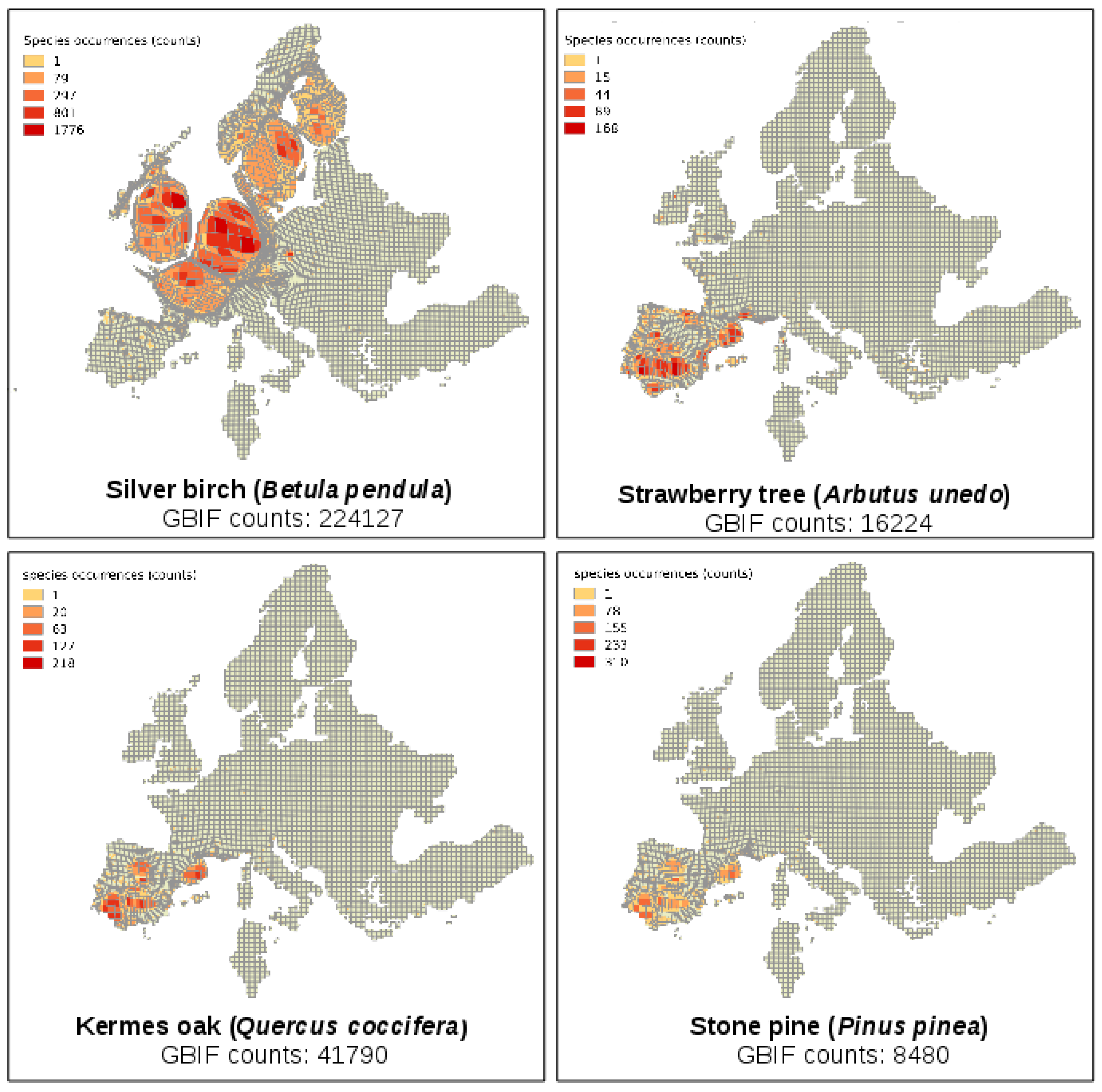
Here, cartograms are used to facilitate the visualization of spatial uncertainty in the results by changing the size of the polygons based on the density of information contained (e.g., number of observations, sampling effort, etc.), thus illustrating the variation in sampling effort and occurrences in field surveys. Using this approach, maps showing the differences in sampling effort (number of different survey dates in the database) and occurrences (observations counts) for a set of plant species over an equal sized grid of Europe were generated (Figure 1). The cartograms were developed using the free and open source software ScapeToad (http://scapetoad.choros.ch/).

The cartograms were generated based on two metrics, number of field surveys (proxy: dates) and number of observations per grid cell. The size of error is given by the size the grid cell should have in terms of the real spatial area it covers, over the actual proportion, as calculated by the number of observations/area. Uncertainty is shown at the per grid cell scale and corresponds to the deformation of the original cell size, that is, cells bigger than their original size required strategies to reduce the effect of oversampling on the products derived from the GBIF data, while cells displayed as smaller than their original size required more sampling efforts. Critically, methods to account for the differences in sampling effort and occurrences (e.g., [26]) may be used to enhance a mapping activity.

4. Mislabelled Training Cases

The effect of mislabelled cases in training datasets was explored using a set of classifiers. The set of classifiers used included contemporary. State-of-the-art approaches such as SVM, RVM, and SMLR, together with a conventional statistical classifier, a discriminant analysis (DA), as a benchmark. Training sets of varying nature were generated and the key aspects of the study design and results are presented in the following sub-sections.

4.1. Data and Methods

A series of supervised classifications were undertaken using airborne thematic mapper (ATM) data acquired for a test site near Feltwell in the United Kingdom. This is a topographically flat test site that is composed mainly of large agricultural fields, each of which had been planted with a single crop type at the time of the ATM data acquisition (Figure 2). The ATM is a standard multispectral scanning system that acquires data in 11 spectral wavebands. Here, the spatial resolution of the imagery was much smaller than the typical field size, reducing aspects of the mixed-pixel problem and so the potential for ambiguous class membership. Samples of the data were input to a series of supervised image classifications using a range of classifiers, from conventional statistical classifiers to contemporary machine learning methods.

To simplify the analyses and aid the acquisition of sufficient training data, only the data acquired in three wavebands, those located at 0.60–0.63, 0.69–0.75, and 1.55–1.75 μm, which had been identified in earlier studies (e.g., [38]) as providing a high degree of class separability, were used. Here, attention focused on the six crop classes that dominated the region at the time of the ATM data acquisition: sugar beet (S), wheat (W), barley (B), carrot (C), potato (P), and grass (G). Following the widely used 30p heuristic, where p is the number of discriminating variables that is often used with statistical classifiers [39], a training set comprising at least 90 cases for each class was required. Here, a total of 100 pixels of each class were randomly obtained from the ATM data and used to form a training set (n = 600). This initial training set is balanced, with each class equally represented, and was taken to be perfect or error-free. The location of the six classes in the three waveband feature space is shown for these training data in Figure 3.

The ATM data were classified using a SVM, RVM, and SMLR as well as standard quadratic discriminant analysis. The latter is a standard statistical classifier that uses summary statistics for each class derived from the training data, while the other three classifiers use the available training cases differently. Details on the algorithms are given below, but it is important to note that the SVM, RVM, and SMLR focus on different cases in the training set [35], with each typically using only a subset of all available cases; the subset used may differ greatly between the classifiers. For example, the RVM and SVM may both make use of relatively atypical training cases but are drawn from markedly different locations of feature space [35]. To find the optimal values of user-defined parameters (

Table 1. User-defined parameters with ATM data using different classifiers.

Classifier
SVM		RVM		SMLR
C	λ	α	λ	β	λ
65.536	8.192	1.0e9	0.50	0.70	0.50

) for the error free training data with the different algorithms, 5-fold cross-validation with SVM and the trial and error method with RVM and SMLR were used; these values were used throughout.

A series of classifications were undertaken using training sets of variable quality. In each classification the size of the training set was constant. The initial training dataset was assumed to be error-free and a series of training sets of variable quality was obtained from it by controlled degradation following two strategies. In both strategies the class label for the training cases that lay closest to the border position between two classes in feature space, identified from the set of Mahalanobis distances to class centroids for each case [22], was altered; the focus is, therefore, on the border area between classes in feature space that is likely to furnish support vectors. Specifically, the difference between the Mahalanobis distance to the two spectrally closest classes was used as a simple means to identify border cases that lie between classes [22]. The training cases for each class were ordered by the difference in this distance and a percentage of the cases with the smallest distance relabelled to form the imperfect training sets. In the first strategy, the class label was altered from the actual class to that of the second most likely class of membership and so the error is between relatively similar classes. In the second strategy, the label was altered from the actual class to that of a class chosen at random. Both strategies were used to form a series of training sets in which the magnitude of mislabelled cases was 5%, 10%, and 20% of the total training set size. Throughout, therefore, the focus is on mislabelling of what may be thought of as border cases rather than, for example, randomly selected cases.

The accuracy of each classification was assessed using a single testing dataset. This testing set was formed using stratified random sampling with 75 cases per class (n = 450). Note that this size of testing set exceeds the widely used suggestion that at least 50 cases per class be used. The accuracy of each classification was assessed and expressed as the proportion of correctly allocated cases obtained from the confusion matrix. The statistical significance of differences in the magnitude of the estimated overall accuracy of classifications was also evaluated using the McNemar test at the 95% confidence level [40]. Additionally, in recognition of the need to accommodate for the sample design used, for individual classes, the confidence interval around estimates of accuracy obtained was used to evaluate the statistical significance of differences in accuracy [41].

4.2. Classifiers

Four classification algorithms were used: discriminant analysis, SVM, RVM, and SMLR. The salient details of each of the classifiers are provided below. This discussion draws, in part, on a previous article [35] that also provides fuller details on the SVM, RVM, and SMLR. In the discussion about different classification algorithms, a training dataset $\left({\mathit{x}}_i, {\mathit{y}}_i\right),$ i = 1, …, n, having n number of samples, where $x={\left[{\mathrm{x}}_1,{\mathrm{x}}_2,\dots ,{\mathrm{x}}_{\mathrm{f}}\right]}^{\mathrm{T}}\in R^{\mathrm{f}}$ is input vector with f spectral features and $\mathit{y}= {\left[y_1, y_2,\dots , y_q\right]}^{\mathrm{T}}\in R^q$ is the class vector with q classes, is used.

4.2.1. Discriminant Analysis

Discriminant analysis is widely used in the classification of remotely sensed data [42,43]. It is a conventional statistical classifier which allocates each case to the class with which it displays the highest a posteriori probability of membership. The latter may be derived from

$$L \left(c|x\right)=P_c p\left(x|c\right)/{\displaystyle \sum }_{j=1}^q{P}_j p\left(x|j\right)$$

(1)

where $L \left(c|x\right)$ is the posterior probability of case x belonging to class c, $p\left(x|c\right)$ is the typicality probability (the probability that case x would be a member of class c given the distance it is from the centroid of class c), P_c is the a priori probability for class c, and q is the total number of classes. The typicality probability is calculated from the Mahalanobis distance, D, between a case and the centroid of a class from

$$D^2= {\left({\mathit{x}}_f- {\mathit{u}}_c\right)}^{\mathrm{T}}{\mathit{v}}_c^{-1}\left({\mathit{x}}_f- {\mathit{u}}_c\right)$$

(2)

where ${\mathit{x}}_f$ is the data vector for the pixel, ${\mathit{v}}_c$ is the variance–covariance matrix for class c, and ${\mathit{u}}_c$ is the mean vector for class c [39].

4.2.2. SVM

The SVM aims to determine the location of class boundaries that produce the optimal separation of classes [44] based on statistical learning theory. For a two-class linearly separable classification problem, the SVM selects the linear decision boundaries that provide the greatest margin between the two classes, where the margin is defined as the sum of the distances to the hyperplane from the closest points of the two classes [44]. SVM use a standard quadratic programming optimisation technique to solve the problem of maximising the margin between two classes and the class cases closest to the hyperplane used to measure the margin are called ‘support vectors’. These support vectors, being a small proportion of the total training set, are atypical in nature and lie in the border region between classes [32,35].

In case of linearly non-separable classes, the SVM selects a hyperplane that maximises the margin, while at the same time minimising a quantity proportional to the number of misclassification errors. A slack variable is introduced to relax the restriction that all training cases of a given class lie on the same side of the optimal hyperplane and the trade-off between margin and misclassification error is controlled by a positive user-defined constant C (a regularization parameter) such that ∞ > C > 0 [27].

To handle non-linear decision boundaries with SVM, an approach of projecting the input data onto a high-dimensional feature space through nonlinear mapping was proposed by [45]. This approach allows a linear classification problem to be framed in the new feature space. The major challenge in solving SVM problems in this high-dimensional feature space is the huge computational cost. To deal with this high-dimensional feature space and reduce the computational cost, use of a kernel function, satisfying the Mercer’s theorem, was suggested by [27]. A kernel function is defined as $K\left(x_i, x_j\right)= \Phi \left(x_i\right).\Phi \left(x_j\right)$ and the hypothesis space for SVM using a kernel function can be defined as:

$$f\left(x\right)= \mathrm{sign}\left({\displaystyle \sum }_i{\lambda }_i{y}_i K\left(x_i, x_j\right)+\mathrm{b}\right)$$

(3)

where ${\lambda }_i$ is a Lagrange multiplier. Further and more detailed discussion of SVM can be found in [44] and [45]. The SVM analyses reported in this article are different to those reported in an earlier study [46], with all analyses repeated mainly so that information on additional, but previously unrecorded, features such as the number of support vectors could be obtained.

4.2.3. RVM

The RVM, also a kernel-based machine learning algorithm, is based on a Bayesian formulation of a linear model with an appropriate prior [47]. The RVM is considered a probabilistic counterpart to the SVM and effectively used as an alternative to SVM for remote sensing image classification [48,49,50]. RVM is based on a hierarchical prior, where an independent Gaussian prior is defined on the weight parameters and an independent Gamma hyper prior is used for the variance parameters in the first and second levels, respectively [47]. This results in an overall student-t prior on the weight parameters, which leads to a sparse solution [47]. Ability to use non-Mercer kernels, probabilistic output, and no need to define the regularisation parameter (C) are some of the key advantages of the RVM over the SVM [35]. In a two-class classification by RVM, the aim is, essentially, to predict the posterior probability of membership for one of the classes for a given input. A case may then be allocated to the class with which it has the greatest likelihood of membership. Using a Bernoulli distribution, the likelihood function for the analysis would be:

$$p \left(y|g\right)= {\displaystyle \prod }_{i=1}^n\sigma {\left\{\left(y\left(x_i\right)\right)\right\}}^{y_i}{\left[1-\mathsf{\sigma }\left\{\left(y\left(x_i\right)\right)\right\}\right]}^{1-y_i}$$

(4)

An iterative method is used to obtain $p \left(y|g\right)$. Let ${\mathsf{\alpha }}_i^{*}$ denotes the maximum a posteriori estimate of the hyperparameter ${\mathsf{\alpha }}_i$. The maximum a posteriori estimate of the weights $\left(g_{MAP}\right)$ can be obtained by maximizing the following objective function:

$$\mathrm{f}\left({\mathrm{g}}_1,{\mathrm{g}}_2,\dots , {\mathrm{g}}_n\right)= {\displaystyle \sum }_{i=1}^n\log p \left(y_i|g_i\right)+{\displaystyle \sum }_{i=1}^n\log p \left(g_i|{\alpha }_i^{*}\right)$$

(5)

The first summation term in Equation (5) corresponds to the likelihood of the class labels and the second term corresponds to the prior on the parameters $g_i$. The gradient of function f with respect to g is calculated for the solution of Equation (5) and only those training cases having non-zero coefficients $g_i$, called relevance vectors, contribute to the generation of a decision function.

An iterative process, in which the hyperparameters ${\alpha }_i$ associated with each weight are updated, is used to find the set of weights by maximizing the value of Equation (5). During the training process of RVM, the hyperparameter ${\alpha }_i$ will attain very large value for a large number of training cases and the associated weights will be reduced to zero. This process makes most of the training case irrelevant to the classification problem and results in a subset of useful training cases being used for final classification. As with the SVM, these useful training cases tend to be atypical but, unlike the SVM, they also have an anti-boundary nature [35,47]. Further details on the RVM are provided in [47].

4.2.4. SMLR

The Sparse Multinomial Logistic Regression algorithm (SMLR; [51]) is a multiclass classifier based on the multinomial logistic regression. This classifier enforces sparsity using a Laplacian prior on the weights of the linear combination of functions. Laplacian prior supports few large weights whereas most of the others are set to exactly zero.

If ${\mathit{w}}_c$ is the weight vector associated with class c, then the probability that a given training case x belongs to class can be defined by

$$P\left(y_c= 1/x, \mathit{w}\right)= \frac{exp\left({\mathit{w}}_c^T x\right)}{{{\displaystyle \sum }}_{c=1}^{q}exp\left({\mathit{w}}_c^T x\right)}$$

(6)

Usually a maximum likelihood estimation procedure is used to obtain the components of $\mathit{w}$ from the training data by maximizing the log-likelihood function [52] defined as:

$$l\left(w\right)= {\displaystyle \sum }_{k=1}^n\left[{\displaystyle \sum }_{c=1}^q{y}_{ck}{w}_c^T{x}_k- log{\displaystyle \sum }_{c=1}^q\exp \left(w_c^T{x}_k\right)\right]$$

(7)

To achieve sparsity during the training process, SMLR uses a Laplacian prior $\left(l_1\right)$ and, to estimate w, a maximum a posteriori (MAP) criterion as proposed by [39] is used:

$${\mathit{w}}_{MAP}=\underset{w}{\arg \max }\left[l\left(\mathit{w}\right)+\log lap\left(\mathit{w}\right)\right]$$

(8)

where $lap\left(\mathit{w}\right)$ is a Laplacian prior on w and can be defined as $lap\left(\mathit{w}\right) \mathit{\alpha } exp \left(-\mathit{\beta } {\Vert \mathit{w}\Vert }_{\mathbf{1}}\right)$, with $\mathit{\beta }$ a user-defined parameter that controls the level of sparsity. Further details can be found in [51].

4.3. Results and Discussion

The classifications based upon the original, assumed to be error-free, training set showed that the classification from SVM (89.11%) was slightly more accurate than all of the other classifications; the accuracy of the classification from the discriminant analysis, RVM, and SMLR were 86.88%, 88.0%, and 88.67%, respectively. This outcome is compatible with discussions in the literature and confirms the potential of SVM-based classification that has been widely reported in the literature. The confusion matrices for the classifications obtained using the error-free training set are shown in

Table 2. Confusion matrices for classifications using error-free training data: (a) SVM; (b) RVM; (c) SMLR; and (d) discriminant analysis. Columns show reference data and rows the classification labels. Also shown are user’s (User) and producer’s (Prod) accuracy. Classes are defined in Section 4.1.

(a)		S	W	B	C	P	G	Σ	User (%)
	S	62	3	4	1	1	0	71	87.32
	W	4	65	3	0	3	0	75	86.67
	B	5	7	68	0	0	1	81	83.95
	C	1	0	0	70	5	0	62	92.11
	P	3	0	0	0	62	0	76	95.38
	G	0	0	0	4	4	74	65	90.24
	Σ	75	75	75	75	75	75
Prod (%)		82.67	86.67	90.67	93.33	82.67	98.67
(b)		S	W	B	C	P	G	Σ	User (%)
	S	62	5	2	1	2	0	72	86.11
	W	3	66	5	0	4	0	78	84.62
	B	5	4	68	0	0	1	78	87.18
	C	1	0	0	70	5	2	78	93.75
	P	4	0	0	0	60	2	66	90.91
	G	0	0	0	4	4	70	78	92.21
	Σ	75	75	75	75	75	75
Prod (%)		82.67	88.00	90.67	93.33	80.00	93.33
(c)		S	W	B	C	P	G	Σ	User (%)
	S	63	4	1	1	2	0	71	88.73
	W	4	69	10	0	4	0	87	79.31
	B	3	2	64	0	0	0	69	92.75
	C	1	0	0	72	5	4	82	87.80
	P	4	0	0	0	60	0	64	93.75
	G	0	0	0	2	4	71	77	92.21
	Σ	75	75	75	75	75	75
Prod (%)		84.00	92.00	85.33	96.00	80.00	94.67
(d)		S	W	B	C	P	G	Σ	User (%)
	S	61	4	0	1	0	0	66	92.42
	W	4	69	13	1	4	0	91	75.82
	B	3	2	62	0	0	0	67	92.53
	C	1	0	0	70	2	10	83	84.33
	P	6	0	0	1	65	1	73	89.04
	G	0	0	0	2	4	64	70	91.43
	Σ	75	75	75	75	75	75
Prod (%)		81.33	92.00	82.66	93.33	86.66	85.33

. However, here the focus is on the effect of mislabelled training cases on classification accuracy.

Classifications were undertaken using each training set and classifier. The accuracy with which the testing set cases were classified using each classifier and training set is summarized in

Table 3. Overall classification accuracy for cases mislabelled to a randomly selected class; DA—discriminant analysis. Values in brackets are the number of support vectors, relevance vectors, and useful kernel basis functions used.

Error in Data
	0	5%	10%	20%
SVM	89.11% (203)	89.33% (218)	88.0% (236)	84.66% (266)
RVM	88% (51)	87.56% (45)	87.56% (51)	85.78% (48)
SMLR	88.67% (83)	88.22% (71)	87.77% (85)	86% (74)
DA	86.88%	86.66%	87.11%	85.77%

and

Table 4. Overall classification accuracy for cases mislabelled to a similar class. Values in brackets are the number of support vectors, relevance vectors, and useful kernel basis functions used.

Error in Data
	0	5%	10%	20%
SVM	89.11% (203)	89.33% (218)	87.77% (218)	81.11% (218)
RVM	88% (51)	86.44% (47)	86.0% (47)	82.67% (36)
SMLR	88.67% (83)	87.78% (94)	86.44% (97)	82.67% (98)
DA	86.88%	86.88%	85.55%	83.11%

for the scenarios involving mislabelling to a random class and a similar class, respectively. The key results of each are summarized in confusion matrices for SVM (

Table 5. Confusion matrices for classifications by the SVM using training sets containing cases mislabelled to a randomly selected class: (a) 5% error; (b) 10% error; and (c) 20% error.

(a)		S	W	B	C	P	G	Σ	User (%)
	S	63	4	3	1	3	0	74	85.14
	W	3	67	3	1	4	0	78	85.90
	B	5	4	69	1	0	1	80	86.25
	C	1	0	0	68	3	0	72	94.44
	P	3	0	0	0	61	0	64	95.31
	G	0	0	0	4	4	74	82	90.24
	Σ	75	75	75	75	75	75
Prod (%)		84.00	89.33	92.00	90.67	81.33	98.67
(b)		S	W	B	C	P	G	Σ	User (%)
	S	63	4	4	1	3	0	75	84.00
	W	2	63	2	1	5	0	73	86.30
	B	5	8	69	1	0	1	84	82.14
	C	1	0	0	69	2	2	74	93.24
	P	3	0	0	0	60	0	63	95.24
	G	1	0	0	3	5	72	81	88.89
	Σ	75	75	75	75	75	75
Prod (%)		84.00	84.00	92.00	92.00	80.00	96.00
(c)		S	W	B	C	P	G	Σ	User (%)
	S	63	5	6	2	6	1	83	75.90
	W	4	67	9	1	4	0	85	78.82
	B	3	3	58	0	0	1	65	89.23
	C	1	0	0	62	2	0	65	95.38
	P	3	0	0	2	58	0	63	92.06
	G	1	0	2	8	5	73	89	82.02
	Σ	75	75	75	75	75	75
Prod (%)		84.00	89.33	77.33	82.67	77.33	97.33

and

Table 6. Confusion matrices for classifications by the SVM using training sets containing cases mislabelled to a similar class: (a) 5% error; (b) 10% error; and (c) 20% error.

(a)		S	W	B	C	P	G	Σ	User (%)
	S	63	4	3	1	3	0	74	85.14
	W	3	66	4	0	4	0	77	85.71
	B	5	5	68	0	0	1	79	86.08
	C	1	0	0	69	2	0	72	95.83
	P	3	0	0	1	62	0	66	93.94
	G	0	0	0	4	4	74	82	90.24
	Σ	75	75	75	75	75	75
Prod (%)		84.00	88.00	90.67	92.00	82.67	98.67
(b)		S	W	B	C	P	G	Σ	User (%)
	S	65	5	3	1	5	0	79	82.28
	W	3	65	5	0	4	0	77	84.42
	B	5	5	67	0	0	1	78	85.90
	C	1	0	0	64	2	0	67	95.52
	P	1	0	0	7	60	0	68	88.24
	G	0	0	0	3	4	74	81	91.36
	Σ	75	75	75	75	75	75
Prod (%)		86.67	86.67	89.33	85.33	80.00	98.67
(c)		S	W	B	C	P	G	Σ	User (%)
	S	62	5	2	1	10	0	80	77.50
	W	4	69	19	1	5	0	98	70.41
	B	5	1	54	0	0	0	60	90.00
	C	1	0	0	61	1	4	67	91.04
	P	3	0	0	11	56	8	78	71.79
	G	0	0	0	1	3	63	67	94.03
	Σ	75	75	75	75	75	75
Prod (%)		82.67	92.00	72.00	81.33	74.67	84.00

), RVM (

Table 7. Confusion matrices for classifications by the RVM using training sets containing cases mislabelled to a randomly selected class: (a) 5% error; (b) 10% error; and (c) 20% error.

(a)		S	W	B	C	P	G	Σ	User (%)
	S	62	5	1	1	3	1	73	84.93
	W	4	66	10	0	4	0	84	78.57
	B	4	4	64	0	0	0	72	88.89
	C	1	0	0	71	3	2	77	92.21
	P	4	0	0	0	61	2	67	91.04
	G	0	0	0	3	4	70	77	90.91
	Σ	75	75	75	75	75	75
Prod (%)		82.67	88.00	85.33	94.67	81.33	93.33
(b)		S	W	B	C	P	G	Σ	User (%)
	S	63	5	1	1	5	0	75	84.00
	W	4	66	10	1	4	0	85	77.65
	B	4	4	64	0	0	0	72	88.89
	C	1	0	0	69	3	2	75	92.00
	P	3	0	0	0	59	0	62	95.16
	G	0	0	0	4	4	73	81	90.12
	Σ	75	75	75	75	75	75
Prod (%)		84.00	88.00	85.33	92.00	78.67	97.33
(c)		S	W	B	C	P	G	Σ	User (%)
	S	64	5	3	1	9	0	82	78.05
	W	3	67	9	1	4	0	84	79.76
	B	4	3	63	0	0	0	70	90.00
	C	1	0	0	67	2	4	74	90.54
	P	3	0	0	3	56	2	64	87.50
	G	0	0	0	3	4	69	76	90.79
	Σ	75	75	75	75	75	75
Prod (%)		85.33	89.33	84.00	89.33	74.67	92.00

and

Table 8. Confusion matrices for classifications by the RVM using training sets containing cases mislabelled to a similar class: (a) 5% error; (b) 10% error; and (c) 20% error.

(a)		S	W	B	C	P	G	Σ	User (%)
	S	62	5	4	1	3	0	75	82.67
	W	3	65	7	0	4	0	79	82.28
	B	5	5	64	0	0	1	75	85.33
	C	1	0	0	68	2	3	74	91.89
	P	4	0	0	3	62	3	72	86.11
	G	0	0	0	3	4	68	75	90.67
	Σ	75	75	75	75	75	75
Prod (%)		82.67	86.67	85.33	90.67	82.67	90.67
(b)		S	W	B	C	P	G	Σ	User (%)
	S	62	5	3	1	5	0	76	81.58
	W	3	66	9	1	4	0	83	79.52
	B	4	4	63	0	0	1	72	87.50
	C	1	0	0	68	2	3	74	91.89
	P	5	0	0	4	60	3	72	83.33
	G	0	0	0	1	4	68	73	93.15
	Σ	75	75	75	75	75	75
Prod (%)		82.67	88.00	84.00	90.67	80.00	90.67
(c)		S	W	B	C	P	G	Σ	User (%)
	S	63	5	0	1	9	0	78	80.77
	W	4	68	16	1	5	1	95	71.58
	B	4	2	59	0	0	0	65	90.77
	C	1	0	0	60	1	5	67	89.55
	P	3	0	0	12	56	3	74	75.68
	G	0	0	0	1	4	66	71	92.96
	Σ	75	75	75	75	75	75
Prod (%)		84.00	90.67	78.67	80.00	74.67	88.00

), SMLR (

Table 9. Confusion matrices for classifications by the SMLR using training sets containing cases mislabelled to a randomly selected class: (a) 5% error; (b) 10% error; and (c) 20% error.

(a)		S	W	B	C	P	G	Σ	User (%)
	S	62	4	2	1	3	0	72	86.11
	W	4	69	10	0	4	0	87	79.31
	B	4	2	63	0	0	0	69	91.30
	C	1	0	0	72	4	4	81	88.89
	P	4	0	0	0	60	0	64	93.75
	G	0	0	0	2	4	71	77	92.21
	Σ	75	75	75	75	75	75
Prod (%)		82.67	92.00	84.00	96.00	80.00	94.67
(b)		S	W	B	C	P	G	Σ	User (%)
	S	64	5	3	1	4	0	77	83.12
	W	4	68	11	0	4	0	87	78.16
	B	3	2	61	0	0	0	66	92.42
	C	1	0	0	72	4	4	81	88.89
	P	3	0	0	0	59	0	62	95.16
	G	0	0	0	2	4	71	77	92.21
	Σ	75	75	75	75	75	75
Prod (%)		85.33	90.67	81.33	96.00	78.67	94.67
(c)		S	W	B	C	P	G	Σ	User (%)
	S	64	6	2	1	5	0	78	82.05
	W	4	68	12	0	4	0	88	77.27
	B	3	0	59	0	0	0	62	95.16
	C	1	0	2	68	3	6	80	85.00
	P	3	0	0	1	59	0	63	93.65
	G	0	1	0	5	4	69	79	87.34
	Σ	75	75	75	75	75	75
Prod (%)		85.33	90.67	78.67	90.67	78.67	92.00

and

Table 10. Confusion matrices for classifications by the SMLR using training sets containing cases mislabelled to a similar class: (a) 5% error; (b) 10% error; and (c) 20% error.

(a)		S	W	B	C	P	G	Σ	User (%)
	S	63	5	4	1	3	0	76	82.89
	W	4	69	10	0	4	0	87	79.31
	B	3	1	61	0	0	0	65	93.85
	C	1	0	0	72	3	4	80	90.00
	P	4	0	0	1	62	3	70	88.57
	G	0	0	0	1	3	68	72	94.44
	Σ	75	75	75	75	75	75
Prod (%)		84.00	92.00	81.33	96.00	82.67	90.67
(b)		S	W	B	C	P	G	Σ	User (%)
	S	63	5	3	1	5	0	77	81.82
	W	4	70	14	1	4	0	93	75.27
	B	3	0	58	0	0	0	61	95.08
	C	1	0	0	71	3	5	80	88.75
	P	4	0	0	1	60	3	68	88.24
	G	0	0	0	1	3	67	71	94.37
	Σ	75	75	75	75	75	75
Prod (%)		84.00	93.33	77.33	94.67	80.00	89.33
(c)		S	W	B	C	P	G	Σ	User (%)
	S	63	5	3	1	7	0	79	79.75
	W	4	69	16	1	5	0	95	72.63
	B	4	1	56	0	0	0	61	91.80
	C	1	0	0	62	1	8	72	86.11
	P	3	0	0	11	59	4	77	76.62
	G	0	0	0	0	3	63	66	95.45
	Σ	75	75	75	75	75	75
Prod (%)		84.00	92.00	74.67	82.67	78.67	84.00

), and discriminant analysis (

Table 11. Confusion matrices for classifications by the discriminant analysis using training sets containing cases mislabelled to a randomly selected class: (a) 5% error; (b) 10% error; and (c) 20% error.

(a)		S	W	B	C	P	G	Σ	User (%)
	S	63	4	0	1	0	0	68	92.64
	W	4	70	13	1	5	0	93	75.26
	B	3	1	62	0	0	0	66	93.93
	C	1	0	0	68	1	13	83	81.92
	P	4	0	0	4	65	0	73	89.04
	G	0	0	0	1	4	62	67	92.53
	Σ	75	75	75	75	75	75
Prod (%)		84.00	93.33	82.66	90.66	86.66	82.66
(b)		S	W	B	C	P	G	Σ	User (%)
	S	62	4	0	1	1	0	68	91.17
	W	4	70	13	1	5	0	93	75.26
	B	3	1	62	0	0	0	66	93.93
	C	1	0	0	68	1	9	79	86.07
	P	5	0	0	84	64	0	73	87.67
	G	0	0	0	1	4	66	71	92.95
	Σ	75	75	75	75	75	75
Prod (%)		82.66	93.33	82.66	90.66	85.33	88.00
(c)		S	W	B	C	P	G	Σ	User (%)
	S	62	5	0	1	1	0	69	89.85
	W	4	69	13	1	5	0	92	75.00
	B	4	1	62	0	0	0	67	92.53
	C	1	0	0	66	1	9	77	85.71
	P	4	0	0	6	64	3	77	83.11
	G	0	0	0	1	4	63	68	92.64
	Σ	75	75	75	75	75	75
Prod (%)		82.66	92.00	82.66	88.00	85.33	84.00

and

Table 12. Confusion matrices for classifications by discriminant analysis using training sets containing cases mislabelled to a similar class: (a) 5% error; (b) 10% error; and (c) 20% error.

(a)		S	W	B	C	P	G	Σ	User (%)
	S	63	4	0	1	0	0	68	92.64
	W	4	69	13	1	4	0	91	75.82
	B	3	2	62	0	0	0	67	92.53
	C	1	0	0	68	2	8	79	86.07
	P	4	0	0	4	65	3	76	85.52
	G	0	0	0	1	4	64	69	92.75
	Σ	75	75	75	75	75	75
Prod (%)		84.00	92.00	82.66	90.66	86.66	85.33
(b)		S	W	B	C	P	G	Σ	User (%)
	S	62	4	0	1	2	0	69	89.85
	W	4	69	14	1	4	0	92	75.00
	B	3	2	61	0	0	0	66	92.42
	C	1	0	0	68	3	12	84	80.95
	P	5	0	0	4	63	1	73	86.30
	G	0	0	0	1	3	62	66	93.93
	Σ	75	75	75	75	75	75
Prod (%)		82.66	92.00	81.33	90.66	84.00	82.66
(c)		S	W	B	C	P	G	Σ	User (%)
	S	63	5	0	1	3	0	72	87.50
	W	4	69	17	2	4	0	96	71.87
	B	3	1	58	0	0	0	62	93.54
	C	1	0	0	63	2	10	76	82.89
	P	4	0	0	8	63	4	79	79.74
	G	0	0	0	1	3	61	65	93.84
	Σ	75	75	75	75	75	75
Prod (%)		84.00	92.00	77.33	84.00	84.00	81.33

).

It was evident that ground data error degraded the accuracy of classifications obtained from each classifier. The magnitude of the effect, however, varied between the two strategies used to mislabel the training cases. With the training sets that contained cases that had been mislabelled to randomly selected classes, classification accuracy dropped least, by 1.11%, for the discriminant analysis and most, by 4.22%, for the SVM as the amount of mislabelled cases increased to 20% of the training set (Table 3 and Table 5). With the SVM, the effect of mislabelled cases was very small when only 5% and 10% of the training set was mislabelled but accuracy dropped most when 20% of the training cases were mislabelled. It was also evident that the SVM changed from being the most accurate classification when error-free training data were used to the least accurate when 20% of training cases had been mislabelled (Table 3). The results suggest that discriminant analysis, which uses general summary statistics derived from the training cases, was the most tolerant of the set of classifiers investigated to mislabelled cases.

With the training sets in which cases had been mislabelled to a similar class, the effect of mislabelling was generally larger on the classifications from all four classifiers than when random labels had been used. Again the accuracy of the classifications obtained from all classifiers tended to decrease as the proportion of cases mislabelled in the training set increased and the effect was largest for SVM (Table 4). With the SVM the accuracy declined by 8.00% as the percentage of the training set mislabelled rose to 20%, while the corresponding reduction for the discriminant analysis was the lowest at 3.11%. In addition, for the classifications obtained with the training set containing 20% mislabelled cases, the accuracy of the SVM classification (81.11%) was lower than that from the discriminant analysis (83.77%). As with the situation involving randomly mislabelled cases, the SVM changed from being the most accurate classification when the training set was error-free to the least accurate classification when 20% of the training cases were mislabelled.

The results of the SVM are of particular interest, especially given the prior claim about its relative insensitivity to training data error. It is worth noting that when mislabelling had involved random class selection the difference between the accuracy of the classification with no and that with 20% mislabelled cases was statistically significant. When the mislabelling involved similar classes, the accuracy of the classifications obtained with 5%, 10%, and 20% mislabelled training cases all differed significantly (at the 95% level of confidence) from that obtained when there were no mislabelled cases. This suggests that SVM is sensitive to training data error, especially if the mislabelling involves cases that lie in the border region between the actual and mislabelled class. It was also evident that the effects varied between the classes and could be relatively large. For example, the producer’s accuracy for the grass class declined from 98.67% to 84.00% when 20% of the training cases were mislabelled to the most similar class (Table 6). Similarly, for the barley class the accuracy declined from 90.67% to 72.00% when 20% of the training cases were mislabelled to the most similar class (Table 6). These differences in producer’s accuracy were also significant at the 95% level of confidence. It should be noted, however, that the presence of mislabelled training cases could sometimes increase the accuracy of the classification of individual classes, which with the SVM was apparent for the wheat class, which increased in accuracy by 5.33% when 20% of the training cases were mislabelled to the most similar class. With attention on individual classes, it was also evident that the presence of mislabelled training cases caused different omission and commission errors in the classifications derived from the four classifiers. For example, with the SVM the greatest commission error was associated with grass (has the highest row total in Table 5) when errors were random but with wheat when the errors were with the most similar class (Table 6). The magnitude of the omission and commission errors associated with the classes varied between the classifications from the four classifiers, although the wheat class was often associated with high commission errors (Table 5, Table 6, Table 7, Table 8, Table 9, Table 10, Table 11 and Table 12). A fuller assessment of the impacts of these errors on the land cover maps would have to account for the stratified sample used in forming the confusion matrices as the classes actually vary in abundance across the test site. Critically, the effects of mislabelled training cases differ between the classifications, varying with classifier and error type, and hence the impacts will depend on specific end user needs.

It was also evident that the number of support vectors used in the classifications tended to increase with the proportion of mislabelled training cases. In the classifications with error-free training data, a total of 203 support vectors were used. Thus, this SVM used only approximately one-third of the available training data. However, the number of support vectors used rose to 218, 236, and 266 for the classifications using training sets containing 5%, 10%, and 20% randomly mislabelled cases, respectively. With training cases mislabelled to a similar class, the number of support vectors rose less, to 218, when the percentage of mislabelled cases was 20%. Thus, mislabelling not only generally acted to reduce classification accuracy; it required an increase in support vectors, slightly degrading the potential for accurate classification from small training sets. It was evident that the RVM and SMLR classifications used fewer training cases: typically only 36–98 training cases were needed. Moreover, the number of training cases used was sometimes smaller with the greater percentage of mislabelled cases, notably for RVM.

The result show that classification by SVM is, contrary to some suggestions in the literature (e.g., [30]), sensitive to mislabelling error, indeed more so than a conventional statistical classifier such as discriminant analysis. Here, it must be stressed that the main difference in the conclusion from other work is because the focus here was on mislabelling of cases in the border regions of feature space from which the support vectors are typically drawn. This focus is, however, especially important if seeking to exploit the potential for accurate classification by a SVM with small training sets as the most useful training cases would be expected to come from border regions [32,35]. If small training sets focused on candidate support vectors are to be used effectively in analyses it is evident that mislabelling should be avoided in order to not negatively impact on the accuracy of the resulting classification. This issue is especially important as cases that lie close together in feature space but belong to different classes may have some similarities that could lead to mislabelling (e.g., classes of vegetation that are defined on the basis of a variable such as percent canopy cover). Note also that the results for the SVM were similar to those reported in [46], in which the algorithm parameters were optimized for each analysis and hence not a function of the approach adopted here.

5. Conclusions

Reference datasets used in map production are typically imperfect in some way. In this article it has been stressed that the reference data may have a heterogeneous nature in relation to issues such as sampling effort and may contain errors such as mislabelling. These imperfections can be expected to impact negatively on a mapping project. This is especially the case with the use of contemporary classifiers such as machine learning techniques like SVM. Imbalanced training samples can, for example, impact on SVM, but if the nature of the samples contributed to a reference dataset are known it may be possible to reduce the problem. Mislabelling has been proposed to be less of an issue (e.g., [30]), but here was given particular focus. Here, it was shown that the quality of datasets, in terms of the accuracy of their class labelling, is important in the production of land cover maps from remotely sensed data. Training data are often used as if error-free yet are unlikely to be so. Error may arise from a variety of sources, not just simple, random errors. In many instances error may involve relatively similar classes and be concentrated in the border area between classes in feature space. It was shown that mislabelled training cases drawn from border locations can degrade the accuracy of widely used supervised image classifiers. In particular, it was evident that the magnitude of the effect was a function of the amount of mislabelled cases, the nature of the mislabelling, and the classifier used.

Critically, the results presented show that SVM is, contrary to some discussion in the literature, sensitive to mislabelled training cases, which highlights the need to consider the effect of training data quality on classification by SVM. The key conclusions arising from the results of the analyses performed were:

• Mislabelled training data typically degraded the accuracy of image classification, and especially for SVM.
• The effects of mislabelled training were greater when the mislabelling was to a similar class rather than a randomly selected class.
• The effects of training data error varied between the classes involved.
• The number of support vectors required for a classification increased with training data error.
• The SVM changed from the most accurate to the least accurate of the four classifiers investigated as the training data error rose from 0% to 20%.

With knowledge of training data quality, it should be possible to adjust a classification analysis to reduce the negative impacts associated with mislabelled cases. For example, if there were concerns about relatively spectrally extreme training cases that lie in the border area between classes in feature space (e.g. there may be real similarity between the cases on the ground because they inter-grade with each other and hence are also spectrally similar), these could in some instances be ignored or we could use a classifier that was based on the general description of the classes and so less influenced by individual training cases.

References

1. Dong, M.; Bryan, B.A.; Connor, J.D.; Nolan, M.; Gao, L. Land use mapping error introduces strongly-localised, scale-dependent uncertainty into land use and ecosystem services modelling. Ecosyst. Serv. 2015, 15, 63–74. [Google Scholar] [CrossRef]
2. Foody, G.M. Valuing map validation: The need for rigorous land cover map accuracy assessment in economic valuations of ecosystem services. Ecol. Econ. 2015, 111, 23–28. [Google Scholar] [CrossRef]
3. Costa, H.; Foody, G.M.; Jiménez, S.; Silva, L. Impacts of species misidentification on species distribution modeling with presence-only data. ISPRS Int. J. Geo-Inf. 2015, 4, 2496–2518. [Google Scholar] [CrossRef]
4. Foody, G.M. Ground reference data error and the MIS-estimation of the area of land cover change as a function of its abundance. Remote Sens. Lett. 2013, 4, 783–792. [Google Scholar] [CrossRef]
5. Wilkinson, G.G. Results and implications of a study of fifteen years of satellite image classification experiments. IEEE Trans. Geosci. Remote Sens. 2005, 43, 433–440. [Google Scholar] [CrossRef]
6. Foody, G.M. Status of land cover classification accuracy assessment. Remote Sens. Environ. 2002, 80, 185–201. [Google Scholar] [CrossRef]
7. Global Biodiversity Information Facility (GBIF). Available online: http://www.gbif.org (accessed on 14 February 2015).
8. Powell, R.L.; Matzke, N.; De Souza, C.; Clark, M.; Numata, I.; Hess, L.L.; Roberts, D.A. Sources of error in accuracy assessment of thematic land-cover maps in the Brazilian Amazon. Remote Sens. Environ. 2004, 90, 221–234. [Google Scholar] [CrossRef]
9. Scott, W.A.; Hallam, C. Assessing species misidentification rates through quality assurance of vegetation monitoring. Plant Ecol. 2003, 165, 101–115. [Google Scholar] [CrossRef]
10. Goodchild, M.F. Citizens as sensors: The world of volunteered geography. GeoJournal 2007, 69, 211–221. [Google Scholar] [CrossRef]
11. Goodchild, M.F. Whither VGI? GeoJournal 2008, 72, 239–244. [Google Scholar] [CrossRef]
12. Foody, G.M.; See, L.; Fritz, S.; Van der Velde, M.; Perger, C.; Schill, C.; Boyd, D.S. Assessing the accuracy of volunteered geographic information arising from multiple contributors to an internet based collaborative project. Trans. GIS 2013, 17, 847–860. [Google Scholar] [CrossRef]
13. Carlotto, M.J. Effect of errors in ground truth on classification accuracy. Int. J. Remote Sens. 2009, 30, 4831–4849. [Google Scholar] [CrossRef]
14. Foody, G.M. Assessing the accuracy of land cover change with imperfect ground reference data. Remote Sens. Environ. 2010, 14, 2271–2285. [Google Scholar] [CrossRef]
15. Radoux, J.; Lamarche, C.; Van Bogaert, E.; Bontemps, S.; Brockmann, C.; Defourny, P. Automated training sample extraction for global land cover mapping. Remote Sens. 2014, 6, 3965–3987. [Google Scholar] [CrossRef]
16. Bruzzone, L.; Persello, C. A novel context-sensitive semisupervised SVM classifier robust to mislabelled training samples. IEEE Trans. Geosci. Remote Sens. 2009, 47, 2142–2154. [Google Scholar] [CrossRef]
17. Kotsiantis, S.B. Supervised machine learning: A review of classification techniques. Informatica 2007, 31, 249–268. [Google Scholar]
18. Costa, H.; Foody, G.M.; Boyd, D.S. Integrating user needs on misclassification error sensitivity into image segmentation quality. Photogramm. Eng. Remote Sens. 2015, 81, 451–459. [Google Scholar] [CrossRef]
19. Bischof, H.; Schneider, W.; Pinz, A.J. Multispectral classification of Landsat-images using neural networks. IEEE Trans. Geosci. Remote Sens. 1992, 30, 482–490. [Google Scholar] [CrossRef]
20. Lu, D.; Weng, Q. A survey of image classification methods and techniques for improving classification performance. Int. J. Remote Sens. 2007, 28, 823–870. [Google Scholar] [CrossRef]
21. Kavzoglu, T. Increasing the accuracy of neural network classification using refined training data. Environ. Model. Softw. 2009, 24, 850–858. [Google Scholar] [CrossRef]
22. Foody, G.M. The significance of border training patterns in classification by a feedforward neural network using backpropagation learning. Int. J. Remote Sens. 1999, 20, 3549–3562. [Google Scholar] [CrossRef]
23. Mountrakis, G.; Imand, J.; Ogole, C. Support vector machines in remote sensing: A review. ISPRS J. Photogramm. Remote Sens. 2011, 66, 247–259. [Google Scholar] [CrossRef]
24. Huang, C.; Davis, L.S.; Townshend, J.R.G. An assessment of support vector machines for land cover classification. Int. J. Remote Sens. 2002, 23, 725–749. [Google Scholar] [CrossRef]
25. Pal, M.; Mather, P.M. Support vector machines for classification in remote sensing. Int. J. Remote Sens. 2005, 26, 1007–1011. [Google Scholar] [CrossRef]
26. Graves, S.J.; Asner, G.P.; Martin, R.E.; Anderson, C.B.; Colgan, M.S.; Kalantari, L.; Bohlman, S.A. Tree species abundance predictions in a tropical agricultural landscape with a supervised classification model and imbalanced data. Remote Sens. 2016, 8, 161–174. [Google Scholar] [CrossRef]
27. Cortes, C.; Vapnik, V.N. Support-vector networks. Mach. Learn. 1995, 20, 273–297. [Google Scholar] [CrossRef]
28. Mercier, G.; Lennon, M. Support vector machines for hyperspectral image classification with spectral-based kernels. In Proceedings of the IEEE International Geoscience and Remote Sensing Symposium, Toulouse, France, 21–25 July 2003.
29. Melgani, F.; Bruzzone, L. Classification of hyperspectral remote sensing images with support vector machines. IEEE Trans. Geosci. Remote Sens. 2004, 42, 1778–1790. [Google Scholar] [CrossRef]
30. Townshend, J.R.; Masek, J.G.; Huang, C.; Vermote, E.F.; Gao, F.; Channan, S.; Sexton, J.O.; Feng, M.; Narasimhan, R.; Kim, D.; et al. Global characterization and monitoring of forest cover using Landsat data: Opportunities and challenges. Int. J. Digit. Earth 2012, 5, 373–397. [Google Scholar] [CrossRef]
31. Pal, M.; Foody, G.M. Feature selection for classification of hyperspectral data by SVM. IEEE Trans. Geosci. Remote Sens. 2010, 48, 2297–2307. [Google Scholar] [CrossRef]
32. Foody, G.M.; Mathur, A. Toward intelligent training of supervised image classifications: Directing training data acquisition for SVM classification. Remote Sens. Environ. 2004, 93, 107–117. [Google Scholar] [CrossRef]
33. Meir, G.; Jenkins, J.L.; Nettles, J.L.; Hitchings, H.; Davies, J.W. Enrichment of high-throughput screening data with increasing levels of noise using support vector machines, recursive partitioning, and laplacian-modified naive Bayesian classifiers. J. Chem. Inf. Model. 2006, 46, 193–200. [Google Scholar]
34. An, W.; Liang, M. Fuzzy support vector machine based on within-class scatter for classification problems with outliers or noises. Neurocomputing 2013, 110, 101–110. [Google Scholar] [CrossRef]
35. Pal, M.; Foody, G.M. Evaluation of SVM, RVM and SMLR for accurate image classification with limited ground data. IEEE J. Sel. Top. Appl. Earth Obs. Remote Sens. 2012, 5, 1344–1355. [Google Scholar] [CrossRef]
36. Fritz, S.; See, L. Comparison of land cover maps using fuzzy agreement. Int. J. Geogr. Inf. Sci. 2005, 19, 787–807. [Google Scholar] [CrossRef]
37. Anderson, R.P.; Araujo, M.; Guisan, A.; Lobo, J.M.; Martinez-Meyer, E.; Townsend, A.; Soberon, J. Are Species Occurrence Data in Global Online Repositories Fit for Modelling Species Distributions? In The Case of the Global Biodiversity Information Facility (GBIF), 2016; Final Report of the Task Group on GBIF Data Fitness for Use in Distribution Modelling; Global Biodiversity Information Facility: Copenhagen, Denmark, 2016. [Google Scholar]
38. Foody, G.M.; Arora, M.K. An evaluation of some factors affecting the accuracy of classification by an artificial neural network. Int. J. Remote Sens. 1997, 18, 799–810. [Google Scholar] [CrossRef]
39. Mather, P.M.; Koch, M. Computer Processing of Remotely-Sensed Images: An Introduction, 4th ed.; Wiley: New York, NY, USA, 2011. [Google Scholar]
40. Foody, G.M. Thematic map comparison: Evaluating the statistical significance of differences in classification accuracy. Photogramm. Eng. Remote Sens. 2004, 70, 627–633. [Google Scholar] [CrossRef]
41. Fleiss, J.L.; Levin, B.; Paik, M.C.; Fleiss, J. Statistical Methods for Rates & Proportions, 3rd ed.; Wiley-Interscience: New York, NY, USA, 2003. [Google Scholar]
42. Tom, C.H.; Miller, L.D. An automated land use mapping comparison of the Bayesian maximum likelihood and linear discriminant analysis algorithms. Photogramm. Eng. Remote Sens. 1984, 50, 193–207. [Google Scholar]
43. Lark, R.M. Components of accuracy of maps with special reference to discriminant analysis of remote sensor data. Int. J. Remote Sens. 1995, 16, 1461–1480. [Google Scholar] [CrossRef]
44. Vapnik, V.N. The Nature of Statistical Learning Theory; Springer: Berlin/Heidelberg, Germany, 1995. [Google Scholar]
45. Camps-Valls, G.; Bruzzone, L. Kernel Methods for Remote Sensing Data Analysis; Wiley & Sons: Chichester, UK, 2009. [Google Scholar]
46. Foody, G.M. The effect of mis-labeled training data on the accuracy of supervised image classification by SVM. In Proceedings of the IEEE Internal Geoscience Remote Sensings Symtem, Milan, Italy, 26–31 July 2015.
47. Tipping, M.E. Sparse Bayesian learning and the relevance vector machine. J. Mach. Learn. Res. 2001, 1, 211–244. [Google Scholar]
48. Demir, B.; Ertürk, S. Hyperspectral image classification using relevance vector machines. IEEE Geosci. Remote Sens. Lett. 2007, 4, 586–590. [Google Scholar] [CrossRef]
49. Foody, G.M. RVM-based multi-class classification of remotely sensed data. Int. J. Remote Sens. 2008, 29, 1817–1823. [Google Scholar] [CrossRef]
50. Mianji, F.A.; Zhang, Y. Robust hyperspectral classification using relevance vector machine. IEEE Trans. Geosci. Remote Sens. 2011, 49, 2100–2112. [Google Scholar] [CrossRef]
51. Krishnapuram, B.; Carin, L.; Figueiredo, M.A.T.; Hartemink, A.J. Sparse multinomial logistic regression: Fast algorithms and generalization bounds. IEEE Trans. Pattern Anal. Mach. Intell. 2005, 27, 957–968. [Google Scholar] [CrossRef] [PubMed]
52. Hastie, T.; Tibshirani, R.; Friedman, J. The Elements of Statistical Learning: Data Mining, Inference, and Prediction; Springer-Verlag: New York, NY, USA, 2001. [Google Scholar]
Figure 1. Cartograms of observations of four tree species (data extracted from GBIF). The colour bar corresponds to the number of occurrences per grid cell, and the shape deformation corresponds to differences in sampling effort, that is, smaller cells indicate undersampling while bigger cells indicate oversampling.
Ijgi 05 00199 g001
Figure 2. Extract of the ATM data, in 0.60–0.63 μm waveband, with class type annotated.
Ijgi 05 00199 g002
Figure 3. Location of the classes in the three-dimensional feature space of the dataset selected.
Ijgi 05 00199 g003