Article

Exploring the Relationship between Remotely-Sensed Spectral Variables and Attributes of Tropical Forest Vegetation under the Influence of Local Forest Institutions

1
Ashoka Trust for Research in Ecology and the Environment, Royal Enclave, Srirampura, Jakkur, Bangalore 560064, India
2
Manipal University, Manipal, Udupi 576 104, India
3
Fondazione Edmund Mach, Research and Innovation Centre, Department Biodiversity and Molecular Ecology, 38010 S. Michele All’adige (Trento), Italy
4
Azim Premji University, PES Institute of Technology Campus, Pixel Park, B Block, Electronics City, Beside Nice Road, Hosur Road, Bengaluru 560 100, India
*
Author to whom correspondence should be addressed.
ISPRS Int. J. Geo-Inf. 2016, 5(7), 117; https://doi.org/10.3390/ijgi5070117
Submission received: 25 April 2016 / Revised: 3 July 2016 / Accepted: 11 July 2016 / Published: 14 July 2016
(This article belongs to the Special Issue Spatial Ecology)

Abstract

:
Conservation of forests outside protected areas is essential for maintaining forest connectivity, which largely depends on the effectiveness of local institutions. In this study, we use Landsat data to explore the relationship between vegetation structure and forest management institutions, in order to assess the efficacy of local institutions in management of forests outside protected areas. These forests form part of an important tiger corridor in Eastern Maharashtra, India. We assessed forest condition using 450 randomly placed 10 m radius circular plots in forest patches of villages with and without local institutions, to understand the impact of these institutions on forest vegetation. Tree density and species richness were significantly different between villages with and without local forest institutions, but there was no difference in tree biomass. We also found a significant difference in the relationship between tree density and NDVI between villages with and without local forest institutions. However, the relationship between species richness and NDVI did not differ significantly. The methods proposed by this study evaluate the status of forest management in a forest corridor using remotely sensed data and could be effectively used to identify the extent of vegetation health and management status.

1. Introduction

Ecological research is vital for establishing effective management and conservation policies for the proper governance of natural resources [1]. In particular, evidence-based data on the effectiveness of conservation management typically requires a solid foundation of in-depth fieldwork. Although this is very important, field data collection is a time-consuming and expensive process [2]. It can often be very difficult to acquire field data in remote and inaccessible places, in areas with challenging terrain, or in areas of ongoing conflict and turmoil that may be of high ecological importance.
Remote sensing can be a valuable aid in such contexts. Remote sensing studies are conducted with the aid of satellite images whereas ecological studies involve in-depth field work, which may or may not cover large spatial regions [2]. Predictions based solely on ecological field studies are hence spatially bounded, and often need to be complemented with broad-scale geographic data for extrapolation to the landscape or regional scale [3]. A combination of remote sensing and field-based ecology research has contributed immensely towards understanding ecological processes, since they facilitate research at moderate to large spatial extents in a cost-effective manner [4,5]. Although ecological field based research is not replaceable by remote sensing methods, the two methods complement each other for better understanding of ecological processes. This can further be incorporated in conservation and management plans [6].
Ecological variability (heterogeneity and biodiversity) forms an important indicator of ecosystem function and ecosystem health [7]. Several studies have been carried out to find the relationship between remotely sensed spectral heterogeneity and ecological variability [8,9]. The Normalized Difference Vegetation Index (NDVI) and other vegetation indices have frequently been used as proxies for vegetation health and structure [10,11,12]. Recent studies have also demonstrated the potential for spectral heterogeneity to be used as a proxy for alpha and beta-diversity of an area, helping in the characterization of biodiversity at larger spatial scales [8,13]. However, ecological processes are complex and the relationship with spectral data may not be very straightforward. For example, it is very difficult to assess understory vegetation variability through optical remote sensing, as such images typically capture information largely from the upper canopy. Active remote sensing such as LiDAR (Light Detection And Ranging) technology could provide solutions to this challenge [14] but typically, such images are expensive and often difficult to acquire, particularly in many biodiverse tropical environments [15]. Thus, so far, most studies have been based on moderate resolution images such as the Landsat data archive, which is freely available [16].
Vegetation structure and variability arises not only as a consequence of ecological and bio-physical processes but is also shaped by social, economic and institutional processes [17,18,19]. Studies from Europe have shown that the species richness, number of dead logs and soil nitrogen are higher in unmanaged forest patches compared to managed forest patches and that the forest patches differ in forest structural stages such as understory growth [20,21]. Institutional processes play an important role in impacting vegetation structure and variability, such as management of forest patches within as well as outside protected areas [22,23]. In this context, most research addressing the impact of institutions on forest biodiversity and variability has focused on state-administered protected areas [24,25,26]. Globally, a large extent of forests lies outside protected areas and is managed by various institutional structures. Local community institutions play an important role in maintaining these forest patches [27].
India harbours large, connected forest areas with high plant and animal diversity. A large proportion of India’s forest land is located outside the country’s protected area network [25,28]. Legally, forest patches outside protected areas belong to the state. These forest patches are under the formal control of the Indian Forest Department, but at smaller scales may be managed by local communities through informal institutions such as sacred groves, as well as by traditional norms of local communities that relate to hunting and harvesting of forest resources [29]. Recently, through Joint Forest Management and the Indian Forest Rights Act of 2006, local communities have also received some de jure (formal) rights to access and maintain forest patches [22,30]. However, forests outside protected areas are undergoing rapid changes, given their location in densely populated landscapes and face economic and political pressure [25,28,31]. Conservation of these forest patches is very important for social reasons such as livelihood dependence of local communities, as well as ecological reasons including wildlife protection.
So far, remotely sensed data has been widely used to classify different types of forest and to assess changes in the forest density, diversity and distribution [4,32]. However, understanding the role of local institutions with the aid of remote sensing is comparatively less explored. In this study, we attempt to develop a better understanding of the relationship between spectral and ecological variability under the influence of local institutions. This can help in extrapolating the relationship between institution and vegetation to the regional level so as to provide policy inputs.
The location of this research is in a forest corridor that connects important protected areas such as the Pench Tiger Reserve and the Tadoba-Andhari Tiger Reserve, among several others, within the eastern Maharashtra region. We focus on the forest outside the tiger reserves that are potential corridors for biodiversity [33]. In this landscape, forest patches are managed by diverse institutional settings that range from active involvement of local communities in forest management, to co-management by local communities and the forest department, and management entirely by the forest department, without any participation from local communities. Several common property resource studies have shown that there is a need for local participation in order to achieve larger conservation goals [34,35,36,37]. Previous research in this region has argued that community institutions are important for protection outside protected areas [37]. However, there has been limited assessment of this hypothesis.
In this study, we use Landsat imagery to understand the relationship between spectral heterogeneity and vegetation variability in the presence or absence of local institutions.
The specific objectives are:
  • To explore the relationship between remotely-sensed spectral variables such as the NDVI, and attributes of forest vegetation, in particular of species richness, tree density, and biomass.
  • To investigate how management by local (community) institutions influences vegetation diversity.
  • To examine whether the relationship between remotely-sensed spectral variables and attributes of forest vegetation diversity differ in forests managed with and without the participation of local communities.

2. Material and Methods
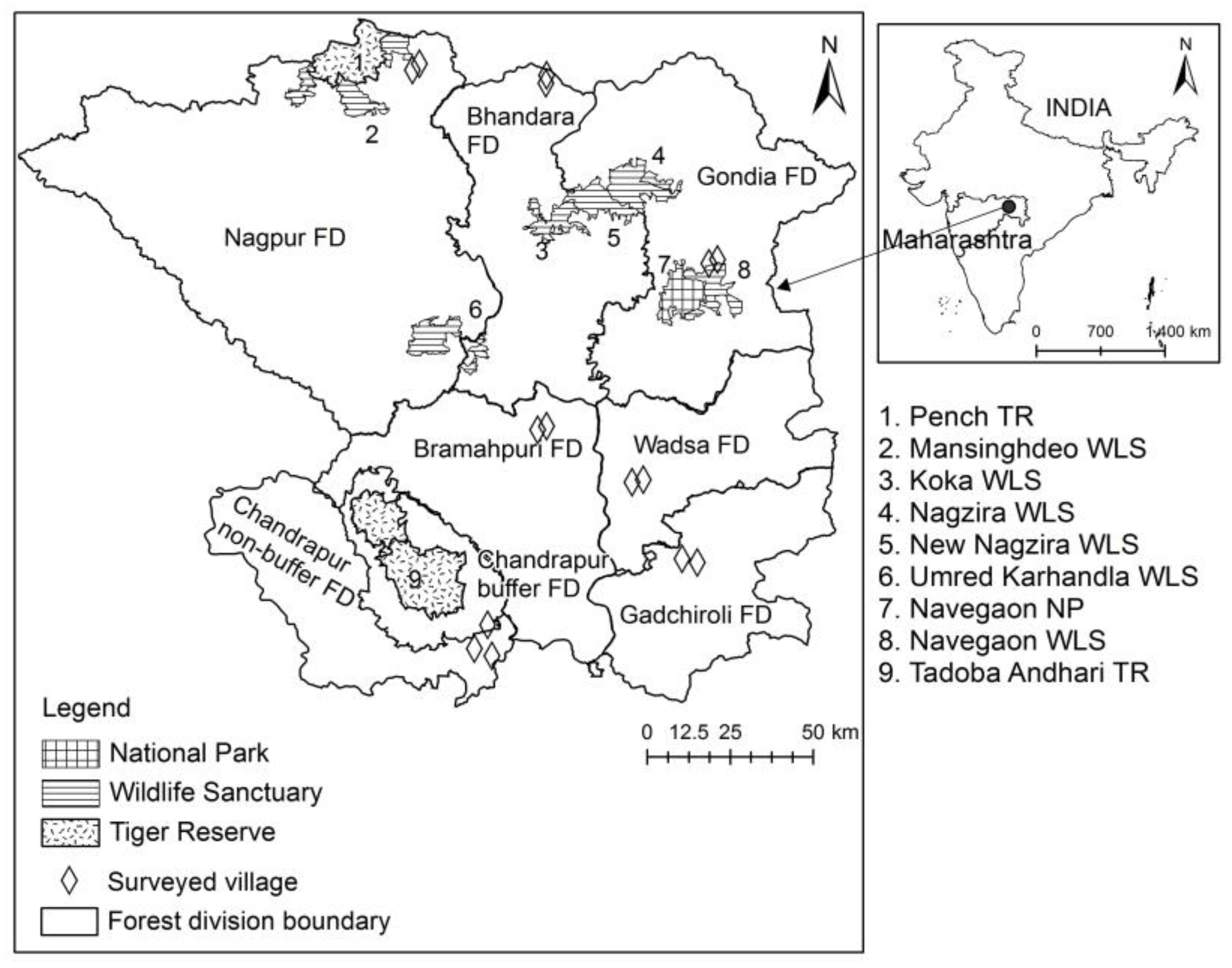
2.1. Study Area

This study was carried out in five forest divisions in Eastern Maharashtra, collectively known as “Vidarbha” (Figure 1). Vidarbha is an underdeveloped region within the state of Maharashtra that has rich dry tropical forest cover and high population density. There are nine protected areas in the selected region with two Tiger Reserves, six Wildlife Sanctuaries and one National Park (Figure 1). Total area under forest cover in the eight forest divisions is around 11,000 km2, out of which only around 1350 km2 is covered by the protected areas. The forest department maintains the forests outside protected areas according to categories such as Reserve Forest and Protected Forest. At times, these are also handed over to the Forest Development Corporation of Maharashtra for management (Table 1).
Approximately thirty-three percent of the population [38] belongs to tribal communities and lives in close proximity to the forest. The tribal as well as non-tribal communities are highly dependent on forests for subsistence and economic livelihoods. Thus, it is very important to understand the interface between local communities, forest use, and conservation of the forest corridor in this region [39]. At the village level, the communities have informally devised rules and regulations for harvesting, managing and protecting the forest resources. At the same time, initiatives of the state such as Joint Forest Management (JFM) schemes and the Forest Rights Act provide limited recognition of rights to local communities for utilization and management of forest patches in their vicinity. Understanding the interplay between these institutions and extent of vegetation within this corridor is very important for maintaining a viable wildlife population. Remote sensing methods provide considerable assistance for covering a regional scale of study.

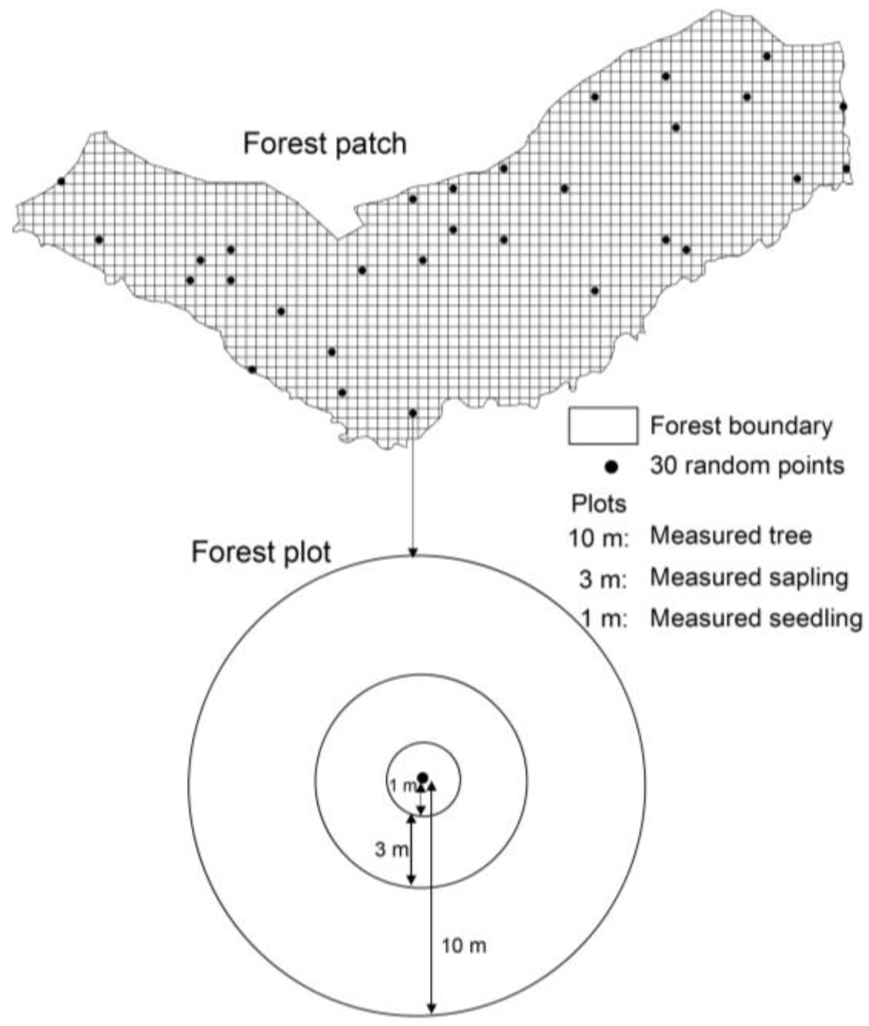
2.2. Field Data Collection

Fieldwork was carried out from October 2013 to February 2014 (during winter), in eight forest divisions (administrative categories) namely Nagpur, Bhandara, Gondia, Brahmapuri, Wadsa, Gadchiroli, Chandrapur buffer and Chandrapur non-buffer. In order to separately manage some forests within the buffer region of Tadoba-Andhari Tiger Reserve (TATR) under the eco-development policy, the Chandrapur forest division was recently divided into buffer and non-buffer forest divisions.
Two villages were selected in each of the eight forest divisions. The snowball sampling method was used to gather information from forest department officials, local NGOs and other key informants regarding local forest institutions. In order to focus on institutional effects, we purposefully selected the villages in such a way that they were similar in terms of population, distance to forest, proximity to market and town, and other facilities. In villages where we found the active participation of local residents in forest management, or where there was joint action by local residents and the forest department in monitoring/managing the forest resource, institutions were categorized as ‘Present’. In villages where peoples’ participation was lacking, either due to the dominance of management by the forest department or with no management of forest resources either by people or by the forest department, institutions were categorized as ‘Absent’. As the Chandrapur Buffer Forest Division has no village without local forest institutions, we have selected 15 villages for this study. Involvement of local people in forest management was subjective and we needed thorough information. Therefore, snowball and purposive sampling methods were used to identify the villages.
Within each of the selected 15 villages, tree density, species richness and tree biomass were estimated using 30 circular forest plots (i.e., a total of 450 plots across the study area) of 10 m radius, within which smaller nested circular plots of 3 m and 1 m radii were used to assess sapling and seedling density and diversity (Figure 2). To select the location of the circular plots, the forest boundaries of each village were mapped and divided into 60 m × 60 m grids, so that the plots were at least be 60 m or two pixels (in case of Landsat image) apart from each other. Then, we randomly selected the 30 grids using the vector tool operation of QGIS [40]. We located each plot in the field by tracking the centroid of each selected grid using a GPS device (GARMIN eTrex Vista, Olathe, KS, USA). We laid circular plots by measuring 10 m radii around the centroid. The projection used was the geographic latitude/longitude World Geodetic System 1984 (WGS84).
In 10 m circular plots, the GBH (Girth at Breast Height) and height of all trees, shrubs and climber species were recorded for all individuals with GBH of more than 10 cm. In 3 m circular plots, the GBH and height of all trees, shrubs, and climber species were recorded for all individuals with GBH less than 10 cm and height more than 1 m. In 1 m circular plots, species identity was recorded for all trees, shrubs, climber species, and herb individuals with height less than 1 m. Later, DBH (Diameter at Breast height) was calculated using GBH. In order to avoid seasonal variation that mostly affects shrub and herb species composition, the data was collected in winter across all villages.
We calculated the tree density, species richness and biomass for each plot. The biomass was calculated using the formula provided by Chave et al. [41], which accounts for tree taper and in which wood density is multiplied by the volume of the cylinder. Wood density data were obtained from Zanne et al. [42] and the Ecosystems Ecology laboratory of the National Centre for Biological Sciences (NCBS), Bangalore, India.

2.3. Remotely Sensed Data

Landsat 8 surface reflectance imagery with a spatial resolution of 30 m, of 14th December 2013 acquisition date were downloaded from the USGS website, to assess the relationship between spectral value and vegetation variability across different sites. This time frame corresponds with the winter time frame (October–February) during which field data was collected. The size of each plot i.e., 10 m radius circular plot is less than the pixel size of 30 m resolution of Landsat 8 images. In order to account for the positional error of around 5–8 m radius, a 3 × 3 pixel window around the central pixel of plot, location was used to calculate the mean and standard deviation of selected indices and bands. This method was used to extract value for Tasseled Cap indices for wetness [43], NDVI and standard deviation of NDVI (SD-NDVI). NDVI is derived from red and infrared bands. NDVI values range between −1 to +1, where high values indicate greener vegetation. Image processing software, ERDAS Imagine™ (9.2, ERDAS Inc., Norcross, GA, USA) was used to calculate NDVI and SD-NDVI; and GRASS GIS 7.0.0RC2 (GRASS Development Team, Michele all'Adige, Italy) was used for Tasseled Cap indices for Wetness.

2.4. Data Analysis

We used quantile regression at very high quantile values (tau = 0.95) to describe the relationship between NDVI and tree density at plots. NDVI is a measure of greenness (or absorption of solar radiation by chlorophyll) and is naturally correlated with the live vegetation cover. This may include any form of vegetation such as grasses, shrubs, or trees. Therefore, the value of NDVI is not limited by tree density alone. In such a case, ordinary least squares regression that describes the relationship between mean of tree density and NDVI is not appropriate. By fitting regression only to higher quantiles of the data, we restrict the prediction to the slice of the data where most NDVI is contributed by standing tree vegetation. Quantile regression is extensively used in various ecological studies, as it helps in estimating the functional relationship between the variables at different quantile values [13,44,45,46]. In ecological studies, it is very difficult to measure all the variables causing an effect, and threshold values are often better described than total variation. Therefore, estimating multiple regression slopes at different quantiles provides greater understanding as compared to ordinary least squares regression [44].
The eight forest divisions within which the villages were present had identical modes of operation and did not have any specific differences in the policies they were implementing. Therefore, while the villages were nested within forest divisions, we did not expect this to have an effect in addition to local conditions. To confirm this assumption we compared tree density, species richness and tree biomass of between villages within each forest division using Mann–Whitney U test (Table A1). In addition, we also compared the same variables between villages, with and without institutions, but pooled across all forest divisions. We expected that the effect of local institutions should be consistent between these two comparisons.
We compared the relationship between spectral and plant community data between villages with and without institutions using regression at a high quantile (0.95). As spectral heterogeneity is a good proxy for beta diversity [46], we also compared the relationship between spectral dissimilarity and beta-diversity in the institution and non-institution villages. The analysis was performed in R 3.2.2 (R Core Team, Vienna, Austria) using package “quantreg version 5.11” for quantile regression [47] and package “vegan version 2.3-1” [48] for dissimilarity indices.

3. Results

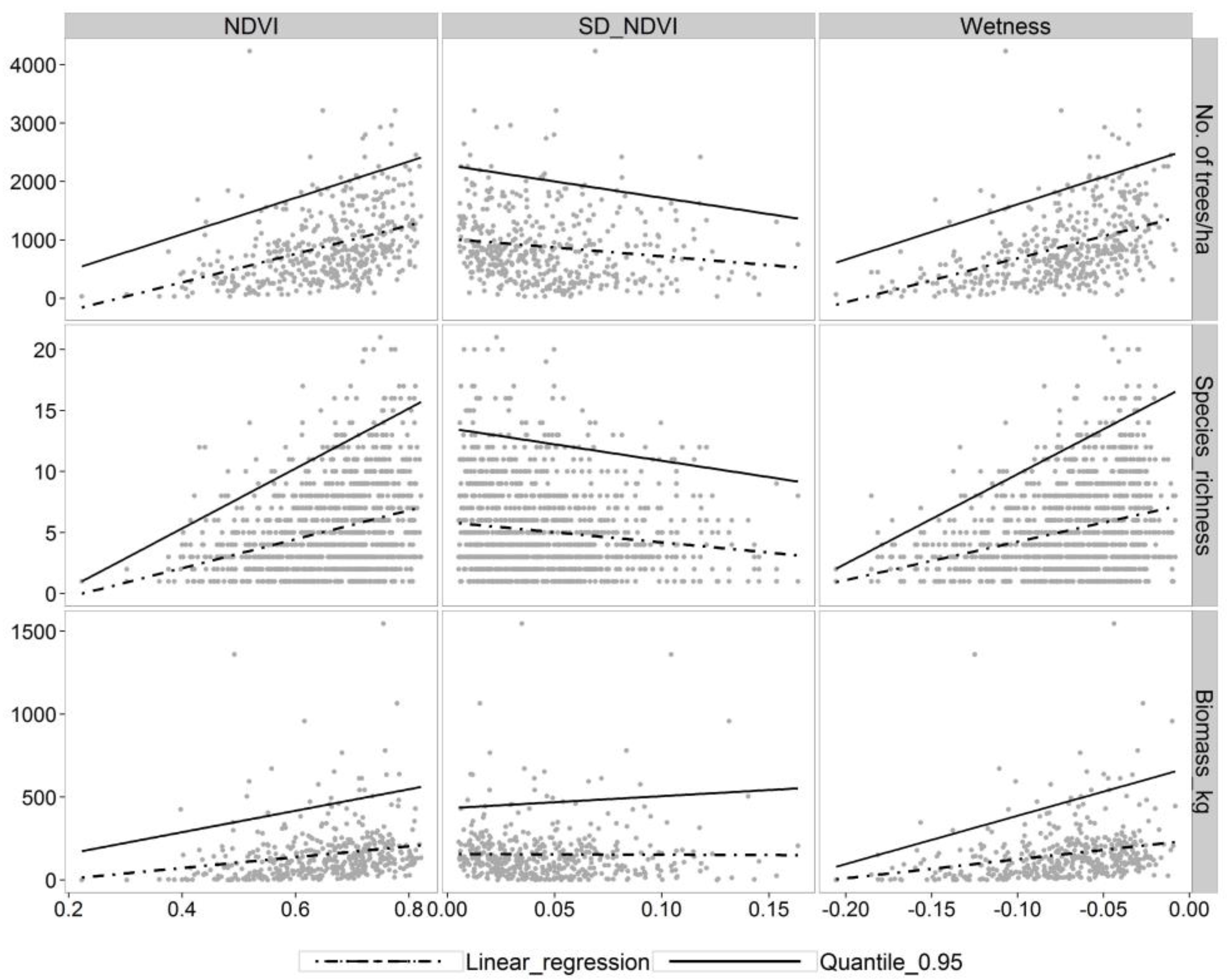
3.1. Relationship between Plant Species and Spectral Diversity

Tree density and richness showed a clear positive relationship with spectral indices and negative relationship with spectral heterogeneity, while the relationship between biomass and the spectral indices was much weaker in both cases. Variance of the response variables also increased with the spectral indices. This is most likely due to the nature of the relationship between spectral indices and tree vegetation (Figure 3).
Tree density, species richness, and biomass were significantly related to spectral values in both quantile and linear regression. Estimates of intercept took more extreme values (positive and negative), and slopes were steeper in quantile regression compared to linear regression. Thus, the relationship between attributes of vegetation and spectral indices varies with the quantile value, and the higher quantiles have a stronger effect than the mean (Figure 3 and Table 2).

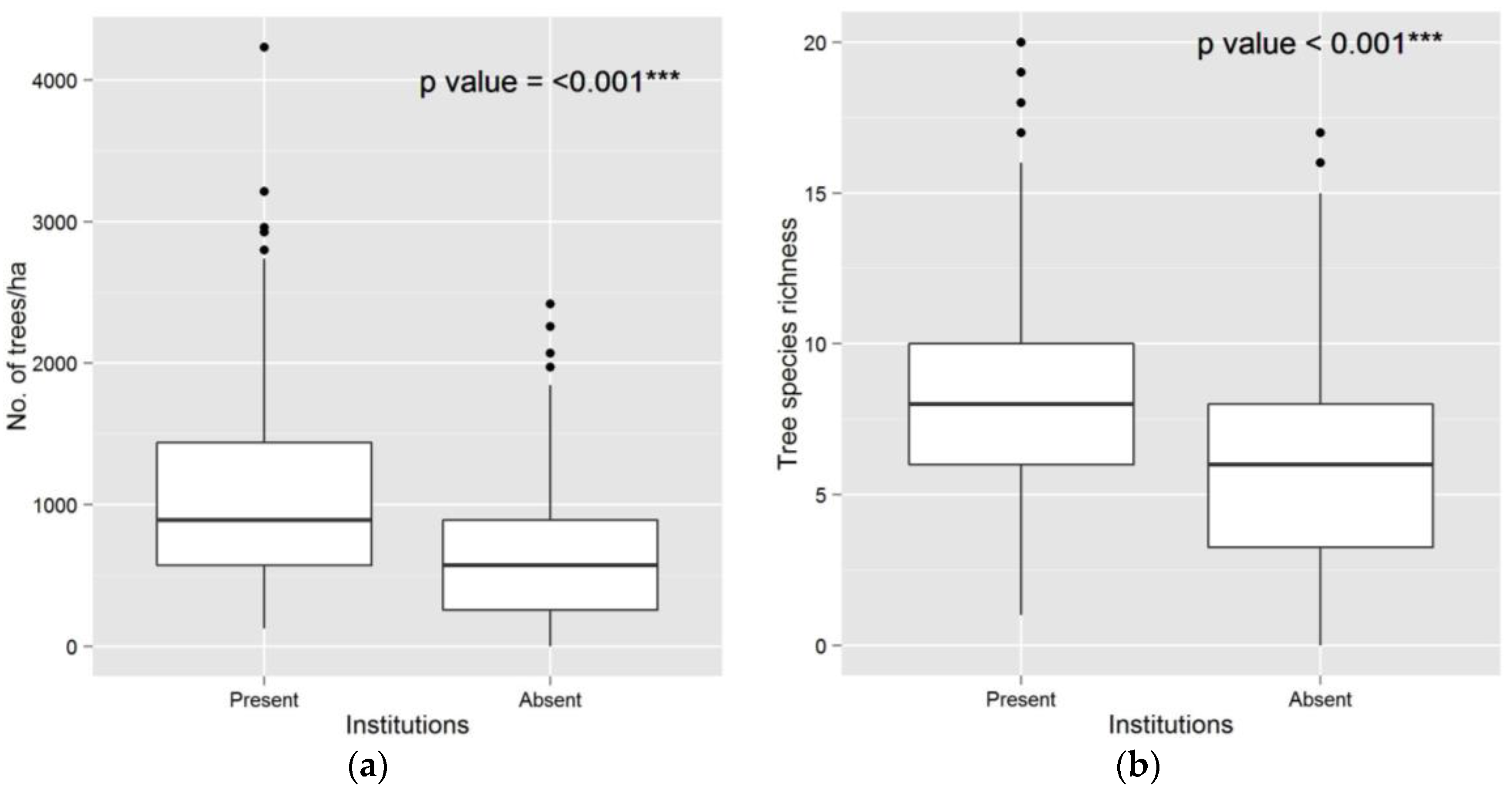
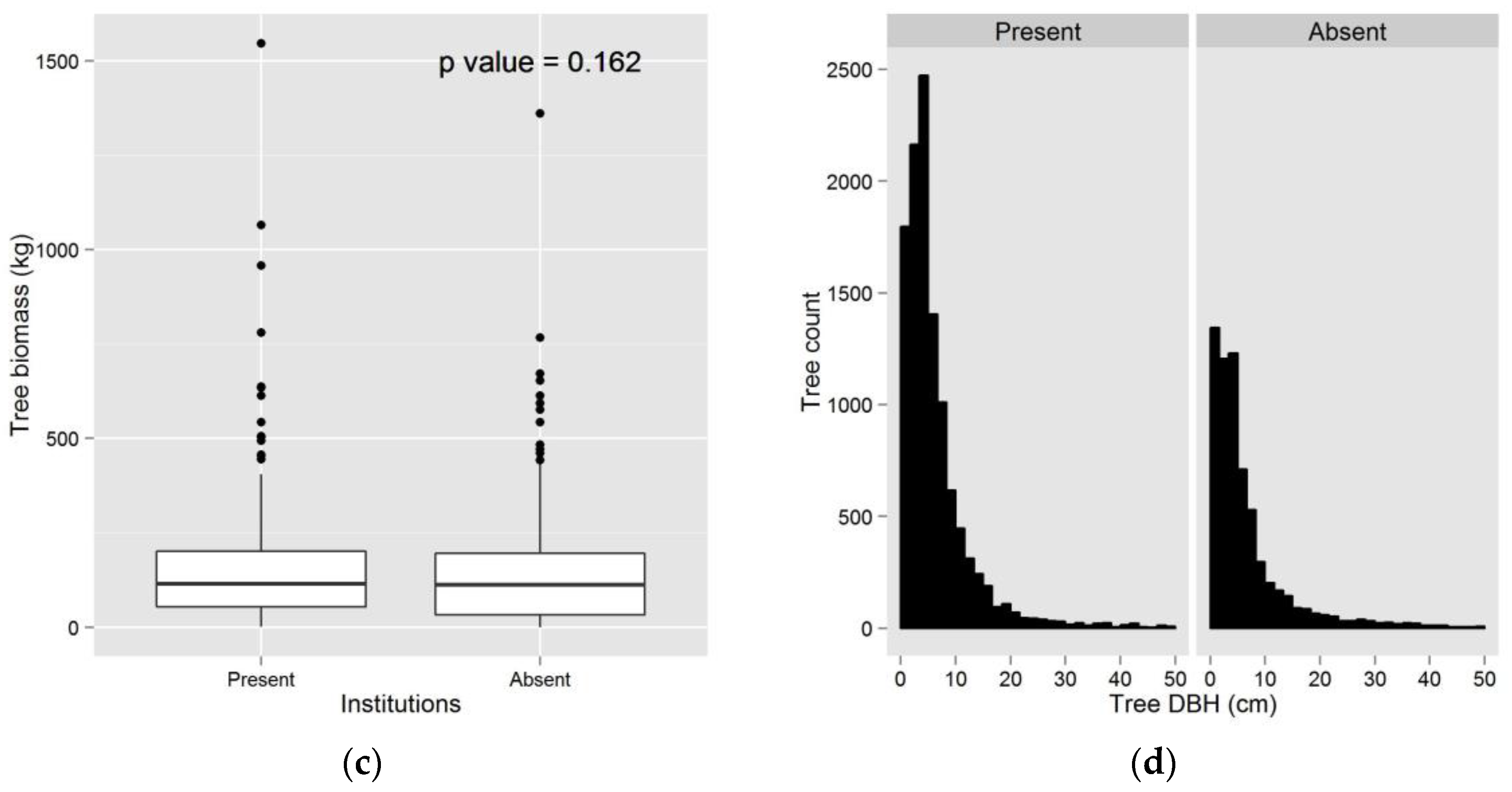
3.2. Impact of Institutions on Plant Species Diversity

Species richness and tree density were higher in villages with institutions as compared to villages without institutions (Figure 4a,b). However, the biomass was the same in different institution settings (Figure 4c). On the other hand, regeneration was high in villages with institutions as compared to villages without institutions (Figure 4d).

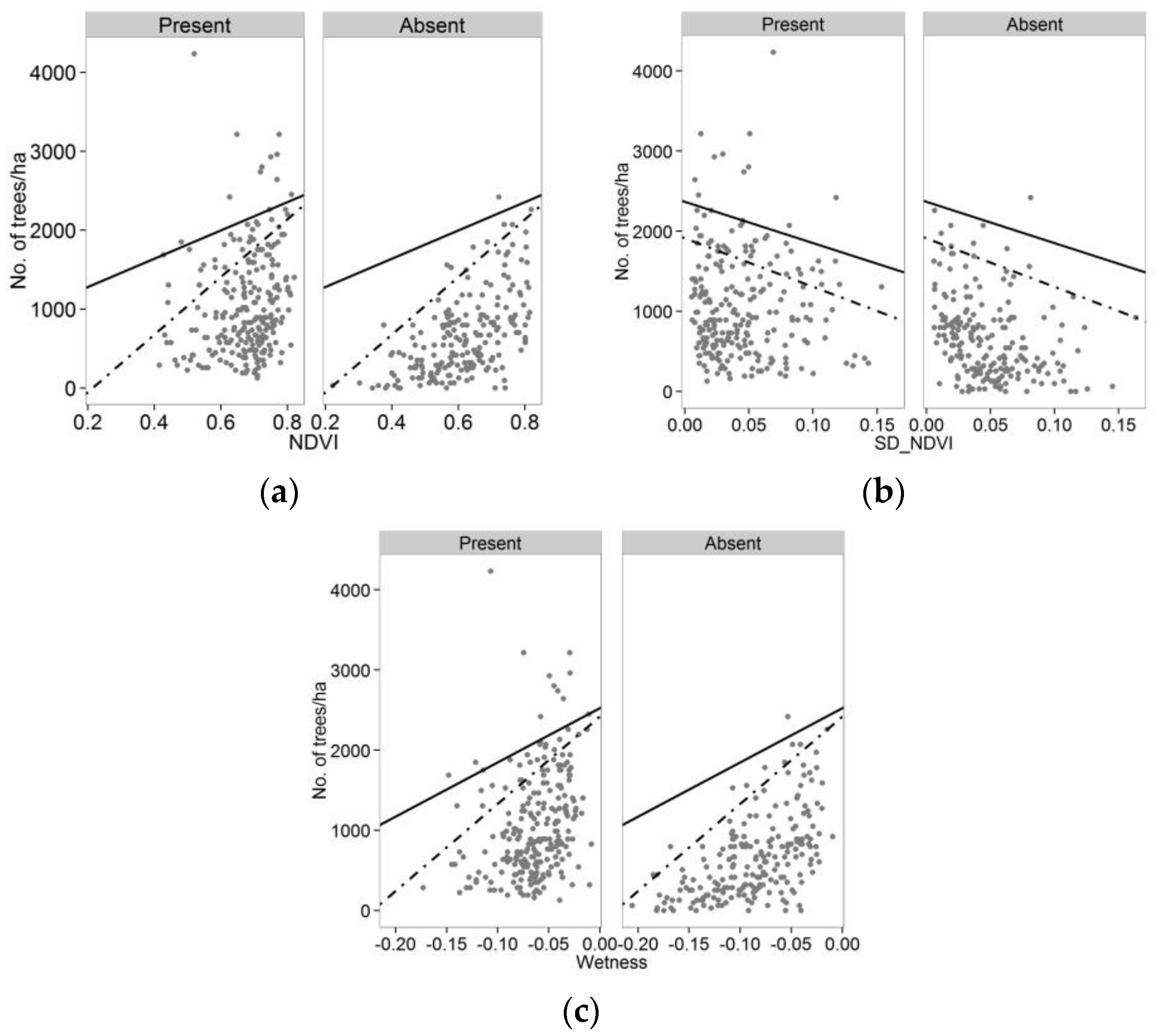
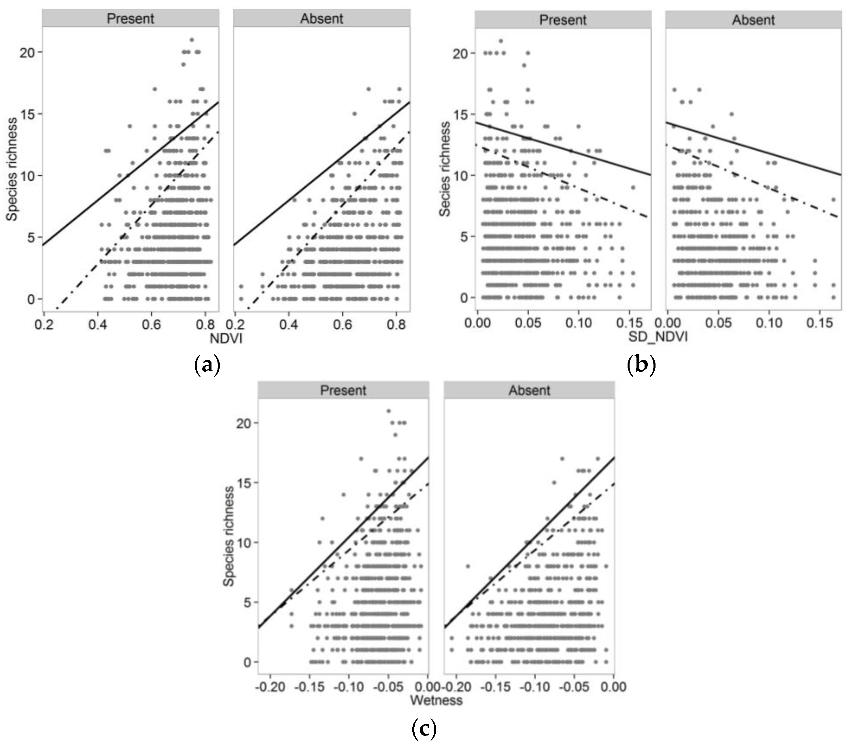
3.3. Relationship between Vegetation Diversity and Spectral Values in Presence and Absence of Forest Institutions

In villages with institutions, the slope of relationship between NDVI and tree density was flatter, and the intercept was higher (Figure 5a); none of the plots recorded an NDVI below 0.4. In contrast, the intercept for villages without institutions was significantly lower as compared to that with institutions (Table 3) and there were some plots that had NDVI below 0.4 (Figure 5a).
The relationship between tree density and SD-NDVI was significantly different in villages with and without forest management institutions (Table 3 and Figure 5b). The relationship between tree density and wetness was not significantly different in villages and without institutions (Table 3 and Figure 5c).
The relationship between species richness and NDVI, SD-NDVI and wetness did not significantly differ between villages with and without institutions (Figure 6 and Table 4). Thus it appears that Landsat remote sensing is more sensitive to tree density, and less able to discern differences in species richness.

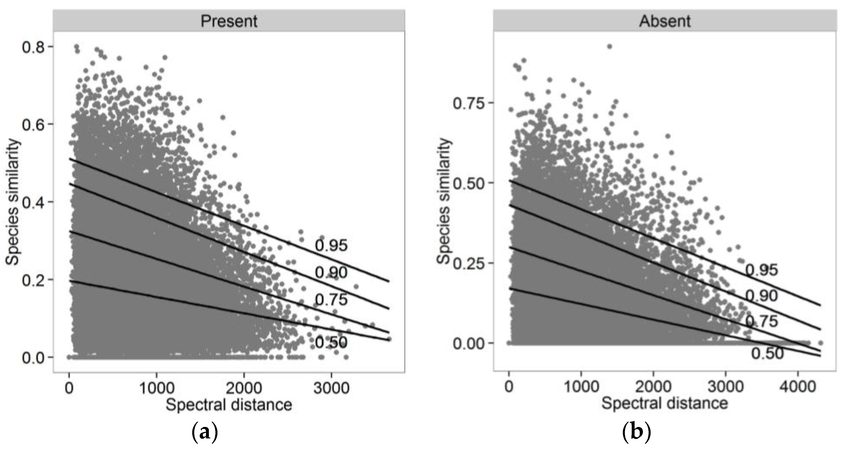
3.4. Relationship between Species Dissimilarity and Spectral Dissimilarity

As the dissimilarity (beta diversity) between species sampled at different locations increases, the spectral distance also increased. A fitted quantile regression line at different quantiles (0.95, 0.90, 0.75, 0.50) was used to help in describing the heterogeneity in tree composition. There was a weak relationship between species similarity and spectral distance. We found no difference in terms of species dissimilarity and spectral dissimilarity in villages with and without institutions (Table 5 and Figure 7).

4. Discussion

Remotely sensed indices such as NDVI, SAVI, SD–NDVI, greenness, and wetness have been previously demonstrated to be useful for the study of vegetation structure, composition and quantification of tree density [9,10,49]. Previous research has utilized remotely sensed data to estimate species richness, diversity, tree density and forest heterogeneity [50,51]. However, dry tropical forests remain relatively less studied as compared to moist tropical forests. In this study of a dry tropical forest in central India, dominated by deciduous species with a relatively open canopy and low-relief topography, we demonstrated relationships between variables of tree composition and density (tree density, species richness and biomass) and spectral values. Specifically, we found that tree density, species richness, and biomass are positively related to NDVI and wetness, and negatively related to SD–NDVI.
We adopted a quantile regression approach to investigate the relationship between spectral indices and forest vegetation. Previous research had demonstrated the use of quantile regression techniques to better capture aspects of ecological variability, as compared to conventional regression approaches [13,46]. We first used quantile regression to set the threshold for tree density, species richness and biomass at a high (0.95 tau) quantile. Setting the relationship to a higher quantile helped in building a relationship with spectral values and the variation contributed by standing trees.
We found significant differences in tree density and species richness between villages with and without forest management institutions, but there was no difference in biomass. Forest patches where local people were involved in management had larger numbers of small trees with DBH less than 15 cm that contributed to the density but did not contribute substantially to woody biomass (Figure 4d). The local institutions in the villages studied were constituted not more than 10–15 years ago. Therefore, the most evident effect of management on vegetation was in terms of increasing the numbers of young trees. If the institutions persist, the biomass in these forests is likely to increase in the future. Given better spatial or spectral resolution data, we may have been able to perceive some of these differences even at this relatively early stage. However, even with Landsat data, we expect that differences in biomass will be visible in a few years, commensurate with the differences in tree density that we observe now.
Given the low rainfall in this climatic zone, trees in these dry deciduous forest areas tended to be slow growing as compared to their moist tropical counterparts where there was a relatively rapid increase in biomass. Studies have shown that the time elapsed since human interventions (including the management, past condition of the forest and intensity of the management) has an effect on forest structure and species composition [20,21]. The differences we observed could be a function of the relative time because of management and the use of forests in different management regimes. Trees in dry tropical forests can take as long as 20 years to regrow [52]. These forest patches could even take longer because of the sustained levels of human use. The density of trees with small DBH can also explain relative differences in the relationship between vegetation attributes and spectral values among villages with and without local institutions. There were a greater number of small trees in the forest patches with institutions as compared to those without institutions. As these small trees are under the canopy, they did not contribute to an increased NDVI value. Therefore, the intercept of the tree density relationship was higher in villages with institutions as compared to those without institutions. However, the relationship between species richness and indices was not significantly different across institutions. The villages shared a large number of similar tree species. Therefore, the difference in species richness across institutions was not clearly captured by remotely sensed data. The relationship between tree density and wetness was also not significantly different across institutions. This could be because the habitat is a dry deciduous forest. Villages with institutions had a greater number of small trees below the upper canopy. Indices of wetness were not able to capture this variation across villages with and without institutions.
Recent studies have shown that as species dissimilarity increases, spectral dissimilarity also increases. We also found a similar relationship between beta diversity and spectral heterogeneity [13,46]. However, we were not able to find any difference in beta diversity in the villages with and without institutions. This could be because the focus of the institutions is not on maintenance of species diversity, in particular of beta diversity. The main focus of these institutions is on protecting their forest patch from excessive tree felling, and on tree plantation. The major difference found in villages with institutions is in terms of regeneration (natural as well as via plantation), which leads to high tree density [53].
Local institutions are known to play an important role in managing common pool resources such as forests [36,54,55]. Understanding functionality of local institutions is very important for conserving forests outside the protected area [55,56]. This study demonstrates that remotely sensed data has the potential to monitor forest outcomes under different management regimes, and to assess the effectiveness of local institutions on different parameters of forest quality such as tree density, biomass, species richness and beta diversity. Such research that integrates ecology, remote sensing and institutional research on forest management is useful for assessing the impact of forest protection outside protected areas—an area that has been insufficiently studied despite its importance. We demonstrated that tree density and species richness could be assessed in tropical forests by using information provided by vegetation indices. Determining a relationship with remotely sensed data can help in developing a better understanding of the role of institutions in forest management, so as to provide better insights for policy. This is particularly relevant in this dry deciduous forest landscape, which is a very important corridor for wildlife, and one that supports local livelihoods. Here, remote sensing methods could serve as an important tool to understand complex socio-ecological processes.

5. Conclusions

This research demonstrated a significant potential of remote sensing for ecological monitoring of how management decisions impact forests. However, a direct relationship with the presence or absence of institutions was difficult to establish, mainly because of scale issues and complexities associated with the functionality of institutions. This may be solved by higher spatial and spectral resolution sensors in future analysis. Specifically, the availability of high temporal resolution data e.g., from the Sentinel-2 constellation will make it possible to use seasonal data for evaluation of forests, while the availability of LiDAR and very high spatial resolution data e.g., Worldview 2/3 will enable the testing of other, less explored proxies such as tree height, canopy structural diversity and texture, all of which can provide important insights in future studies [57].

Acknowledgments

The authors gratefully acknowledge the financial support provided by the South Asian Network for Development and Environmental Economics (SANDEE) under grant number SANDEE/July 2011/008. We thank the Ashoka Trust for Research in Ecology and the Environment (ATREE) for providing lab support and the Maharashtra Forest Division for sharing information. Valuable technical inputs were provided by Jayalakshmi Krishnan, Madhuri Ramesh and Madhura Niphadkar. Neha Mujumdar, Rajkamal Patle, and Vinod Borkar provided excellent assistance during fieldwork. Duccio Rocchini was partially supported by the EU BON (Building the European Biodiversity Observation Network) project, funded by the European Union under the 7th Framework programme (Contract No. 308454), by the ERANET BioDiversa FP7 project DIARS, funded by the European Union, and by the Life project Future for CoppiceS.

Author Contributions

Shivani Agarwal, Duccio Rocchini, and Harini Nagendra conceptualized the research study; Shivani Agarwal conducted the field work; Shivani Agarwal, Aniruddha Marathe and Duccio Rocchini conducted the analysis; and all authors participated in paper writing.

Conflicts of Interest

The authors declare no conflict of interest.

Abbreviations

FDCM
Forest Development Corporation of Maharashtra
JFM
Joint Forest Management
PA
Protected Area
PF
Protected Forest
RF
Reserve Forest
USGS
United State Geological Survey
NDVI
Normalized Difference Vegetation Index
SD-NDVI
Standard Deviation of Normalized Difference Vegetation Index
LiDAR
Light Detection and Ranging
CFM
Community forest management
GBH
Girth at Breast Height
DBH
Diameter at Breast Height
WGS84
World Geodetic System 1984

Appendix

Table A1. Comparison between villages with forest division based on Mann–Whitney U test.
Vegetation Variable Forest DivisionStatisticp Value
Tree density (no. of trees/ha)Bhandara7033.5<00.1***
Brahmapuri7137<00.1***
Chandrapur_non_buffer5994<00.1***
Gadchiroli5701.5<00.1***
Gondia5895<00.1***
Nagpur37890.4
Wadsa6525<00.1***
Species richnessBhandara5980.5<00.1***
Brahmapuri7497<00.1***
Chandrapur_non_buffer5251.5<00.1***
Gadchiroli5242.5<00.1***
Gondia49230.01**
Nagpur36090.2
Wadsa6129<00.1***
Tree biomassBhandara6012<00.1***
Brahmapuri7254<00.1***
Chandrapur_non_buffer31590.01**
Gadchiroli34920.11
Gondia44730.22
Nagpur39780.8
Wadsa2412<00.1***
Significance codes: *** 0.001, ** 0.01.

References

  1. Groom, M.J.; Meffe, G.K.; Carroll, C.R. Principles of Conservation Biology, 3rd ed.; Sinauer Associates: Sunderland, MA, USA, 2006. [Google Scholar]
  2. Kerr, J.T.; Ostrovsky, M. From space to species: ecological applications for remote sensing. Trends Ecol. Evol. 2003, 18, 299–305. [Google Scholar] [CrossRef]
  3. Chambers, J.Q.; Asner, G.P.; Morton, D.C.; Anderson, L.O.; Saatchi, S.S.; Espírito-Santo, F.D.; Palace, M.; Souza, C. Regional ecosystem structure and function: ecological insights from remote sensing of tropical forests. Trends Ecol. Evol. 2007, 22, 414–423. [Google Scholar] [CrossRef] [PubMed]
  4. Nagendra, H. Using remote sensing to assess biodiversity. Int. J. Remote Sens. 2001, 22, 2377–2400. [Google Scholar] [CrossRef]
  5. Newton, A.C.; Hill, R.A.; Echeverría, C.; Golicher, D.; Benayas, J.M.R.; Cayuela, L.; Hinsley, S.A. Remote sensing and the future of landscape ecology. Prog. Phys. Geogr. 2009, 33, 528–546. [Google Scholar] [CrossRef]
  6. Horning, N.; Robinson, J.; Sterling, E.; Turner, W.; Spector, S. Remote Sensing for Ecology and Conservation; Oxford University Press: New York, NY, USA, 2010. [Google Scholar]
  7. Gaston, K.J.; Spicer, J.I. Biodiversity: An Introduction, 2nd ed.; Blackwell Publishing: Oxford, UK, 2004. [Google Scholar]
  8. Rocchini, D. Effects of spatial and spectral resolution in estimating ecosystem α-diversity by satellite imagery. Remote Sens. Environ. 2007, 111, 423–434. [Google Scholar] [CrossRef]
  9. Oldeland, J.; Wesuls, D.; Rocchini, D.; Schmidt, M.; Jürgens, N. Does using species abundance data improve estimates of species diversity from remotely sensed spectral heterogeneity? Ecol. Indic. 2010, 10, 390–396. [Google Scholar] [CrossRef]
  10. Pettorelli, N.; Vik, J.O.; Mysterud, A.; Gaillard, J.-M.; Tucker, C.J.; Stenseth, N.C. Using the satellite-derived NDVI to assess ecological responses to environmental change. Trends Ecol. Evol. 2005, 20, 503–510. [Google Scholar] [CrossRef] [PubMed]
  11. Tucker, C.J.; Pinzon, J.E.; Brown, M.E.; Slayback, D.A.; Pak, E.W.; Mahoney, R.; Vermote, E.F.; El Saleous, N. An extended AVHRR 8-km NDVI dataset compatible with MODIS and SPOT vegetation NDVI data. Int. J. Remote Sens. 2005, 26, 4485–4498. [Google Scholar] [CrossRef]
  12. Pettorelli, N.; Ryan, S.; Mueller, T.; Bunnefeld, N.; Jedrzejewska, B.A.; Lima, M.; Kausrud, K. The Normalized Difference Vegetation Index (NDVI): Unforeseen successes in animal ecology. Climate Res. 2011, 46, 15–27. [Google Scholar] [CrossRef]
  13. Rocchini, D.; Nagendra, H.; Ghate, R.; Cade, B.S. Spectral distance decay: Assessing species beta-diversity by quantile regression. Photogramm. Eng. Remote Sens. 2009, 75, 1225–1230. [Google Scholar] [CrossRef]
  14. Morsdorf, F.; Nichol, C.; Malthus, T.; Woodhouse, I.H. Assessing forest structural and physiological information content of multi-spectral LiDAR waveforms by radiative transfer modelling. Remote Sens. Environ. 2009, 113, 2152–2163. [Google Scholar] [CrossRef] [Green Version]
  15. Nagendra, H.; Rocchini, D. High resolution satellite imagery for tropical biodiversity studies: The devil is in the detail. Biodiv. Conserv. 2008, 17, 3431–3442. [Google Scholar] [CrossRef]
  16. Wulder, M.A.; Masek, J.G.; Cohen, W.B.; Loveland, T.R.; Woodcock, C.E. Opening the archive: How free data has enabled the science and monitoring promise of Landsat. Remote Sens. Environ. 2012, 122, 2–10. [Google Scholar] [CrossRef]
  17. Brechin, S.R.; Wilshusen, P.R.; Fortwangler, C.L.; West, P.C. Beyond the square wheel: Toward a more comprehensive understanding of biodiversity conservation as social and political process. Soc. Nat. Resour. 2002, 15, 41–64. [Google Scholar] [CrossRef]
  18. Ostrom, E.; Nagendra, H. Insights on linking forests, trees, and people from the air, on the ground, and in the laboratory. Proc. Natl. Acad. Sci. USA 2006, 103, 19224–19231. [Google Scholar] [CrossRef] [PubMed]
  19. Holling, C.S. Understanding the complexity of economic, ecological, and social systems. Ecosystems 2001, 4, 390–405. [Google Scholar] [CrossRef]
  20. Paillet, Y.; Bergès, L.; Hjältén, J.; Ódor, P.; Avon, C.; Bernhardt-Romermann, M.; Bijlsma, R.J.; De Bruyn, L.; Fuhr, M.; Grandin, U. Biodiversity differences between managed and unmanaged forests: Meta-analysis of species richness in Europe. Conserv. Biol. 2010, 24, 101–112. [Google Scholar] [CrossRef] [PubMed]
  21. Sitzia, T.; Trentanovi, G.; Dainese, M.; Gobbo, G.; Lingua, E.; Sommacal, M. Stand structure and plant species diversity in managed and abandoned silver fir mature woodlands. For. Ecol. Manag. 2012, 270, 232–238. [Google Scholar] [CrossRef]
  22. Ghate, R.; Nagendra, H. Role of monitoring in institutional performance: forest management in Maharashtra, India. Conserv. Soc. 2005, 3, 509–532. [Google Scholar]
  23. Nagendra, H.; Pareeth, S.; Ghate, R. People within parks—forest villages, land-cover change and landscape fragmentation in the Tadoba Andhari Tiger Reserve, India. Appl. Geogr. 2006, 26, 96–112. [Google Scholar] [CrossRef]
  24. Naughton-Treves, L.; Holland, M.B.; Brandon, K. The role of protected areas in conserving biodiversity and sustaining local livelihoods. Annu. Rev. Environ. Resour. 2005, 30, 219–252. [Google Scholar] [CrossRef]
  25. Karanth, K.K.; DeFries, R. Conservation and management in human-dominated landscapes: Case studies from India. Biol. Conserv. 2010, 143, 2865–2869. [Google Scholar] [CrossRef]
  26. Hayes, T.M. Parks, people, and forest protection: An institutional assessment of the effectiveness of protected areas. World Dev. 2006, 34, 2064–2075. [Google Scholar] [CrossRef]
  27. Coleman, E.A.; Fleischman, F.D. Comparing forest decentralization and local institutional change in Bolivia, Kenya, Mexico, and Uganda. World Dev. 2012, 40, 836–849. [Google Scholar] [CrossRef]
  28. DeFries, R.; Karanth, K.K.; Pareeth, S. Interactions between protected areas and their surroundings in human-dominated tropical landscapes. Biol. Conserv. 2010, 143, 2870–2880. [Google Scholar] [CrossRef]
  29. Fleischman, F. Understanding India’s forest bureaucracy: A review. Reg. Environ. Change 2015, 1–13. [Google Scholar] [CrossRef]
  30. Sarin, M.; Singh, N.M.; Sundar, N.; Bhogal, R.K. Devolution as a Threat to Democratic Decision-Making in Forestry? Findings from Three States in India; Overseas Development Institute: London, UK, 2003. [Google Scholar]
  31. Shahabuddin, G.; Rangarajan, M. Making Conservation Work: Securing Biodiversity in this New Century; Permanent Black: New Delhi, India, 2007. [Google Scholar]
  32. Cohen, W.B.; Goward, S.N. Landsat’s role in ecological applications of remote sensing. BioScience 2004, 54, 535–545. [Google Scholar] [CrossRef]
  33. Joshi, A.; Vaidyanathan, S.; Mondol, S.; Edgaonkar, A.; Ramakrishnan, U. Connectivity of tiger (Panthera tigris) populations in the human-influenced forest mosaic of Central India. PLoS ONE 2013, 8, e77980. [Google Scholar] [CrossRef] [PubMed]
  34. Pretty, J.; Smith, D. Social capital in biodiversity conservation and management. Conserv. Biol. 2004, 18, 631–638. [Google Scholar] [CrossRef]
  35. Ostrom, E. How types of goods and property rights jointly affect collective action. J. Theor. Polit. 2003, 15, 239–270. [Google Scholar] [CrossRef]
  36. Hayes, T.; Ostrom, E. Conserving the world’s forests: Are protected areas the only way? Indiana Law Rev. 2005, 38, 595–617. [Google Scholar]
  37. Ghate, R.; Ghate, S.; Ostrom, E. Can communities plan, grow and sustainably harvest from forests? Econ. Polit. Wkly. 2013, 48, 59–67. [Google Scholar]
  38. Census of India. Available online: http://censusindia.gov.in/ (accessed on 11 October 2014).
  39. Ghate, R.; Ghate, S.; Ostrom, E. Cultural norms, cooperation, and communication: taking experiments to the field in indigenous communities. Int. J. Commons 2013, 7, 498–520. [Google Scholar] [CrossRef]
  40. Team, Q.D. QGIS Geographic Information System, 2015. Open Source Geospatial Foundation Project. Available online: http://qgis.org/ (accessed on 1 September 2013).
  41. Chave, J.; Andalo, C.; Brown, S.; Cairns, M.; Chambers, J.; Eamus, D.; Fölster, H.; Fromard, F.; Higuchi, N.; Kira, T. Tree allometry and improved estimation of carbon stocks and balance in tropical forests. Oecologia 2005, 145, 87–99. [Google Scholar] [CrossRef] [PubMed]
  42. Zanne, A.; Lopez-Gonzalez, G.; Coomes, D.; Ilic, J.; Jansen, S.; Lewis, S.; Miller, R.; Swenson, N.; Wiemann, M.; Chave, J. Global Wood Density Database 2009. Available online: http://datadryad.org/resource/doi:10.5061/dryad.234/1?show=full (accessed on 29 July 2015).
  43. Baig, M.H.A.; Zhang, L.; Shuai, T.; Tong, Q. Derivation of a tasselled cap transformation based on Landsat 8 at-satellite reflectance. Remote Sens. Lett. 2014, 5, 423–431. [Google Scholar] [CrossRef]
  44. Cade, B.S.; Noon, B.R. A gentle introduction to quantile regression for ecologists. Front. Ecol. Environ. 2003, 1, 412–420. [Google Scholar] [CrossRef]
  45. Koenker, R.; Bassett, G., Jr. Regression quantiles. Econometrica 1978, 46, 33–50. [Google Scholar] [CrossRef]
  46. Rocchini, D.; Balkenhol, N.; Carter, G.A.; Foody, G.M.; Gillespie, T.W.; He, K.S.; Kark, S.; Levin, N.; Lucas, K.; Luoto, M. Remotely sensed spectral heterogeneity as a proxy of species diversity: Recent advances and open challenges. Ecol. Inform. 2010, 5, 318–329. [Google Scholar] [CrossRef]
  47. Koenker, R. The Quantreg Package Version 5.11 2015. Available online: https://cran.r-project.org/web/packages/quantreg/index.html (accessed on 29 December 2015).
  48. Oksanen, J.; Blanchet, F.G.; Legendre, P.; Minchin, P.R.; O’Hara, R.B.; Simpson, G.L.; Solymos, P.; Stevens, M.H.H.; Wagner, H. The Vegan Package Version 2.3-1 2015. Available online: https://cran.r-project.org/web/packages/vegan/index.html (accessed on 25 November 2015).
  49. Krishnaswamy, J.; Bawa, K.S.; Ganeshaiah, K.; Kiran, M. Quantifying and mapping biodiversity and ecosystem services: Utility of a multi-season NDVI based Mahalanobis distance surrogate. Remote Sens. Environ. 2009, 113, 857–867. [Google Scholar] [CrossRef]
  50. Nagendra, H.; Rocchini, D.; Ghate, R.; Sharma, B.; Pareeth, S. Assessing plant diversity in a dry tropical forest: Comparing the utility of Landsat and IKONOS satellite images. Remote Sens. 2010, 2, 478–496. [Google Scholar] [CrossRef]
  51. He, K.S.; Zhang, J.; Zhang, Q. Linking variability in species composition and MODIS NDVI based on beta diversity measurements. Acta Oecol. 2009, 35, 14–21. [Google Scholar] [CrossRef]
  52. Murphy, P.G.; Lugo, A.E. Ecology of tropical dry forest. Annu. Rev. Ecol. Syst. 1986, 67, 67–88. [Google Scholar] [CrossRef]
  53. Shahabuddin, G.; Rao, M. Do community-conserved areas effectively conserve biological diversity? Global insights and the Indian context. Biol. Conserv. 2010, 143, 2926–2936. [Google Scholar] [CrossRef]
  54. Ostrom, E. Collective action and the evolution of social norms. J. Econ. Perspect. 2000, 14, 137–158. [Google Scholar] [CrossRef]
  55. Agrawal, A.; Ostrom, E. Collective action, property rights and decentralization in resource use in India and Nepal. Polit. Soc. 2001, 29, 485–514. [Google Scholar] [CrossRef]
  56. Poteete, A.R.; Ostrom, E. Heterogeneity, group size and collective action: the role of institutions in forest management. Dev. Chang. 2004, 35, 435–461. [Google Scholar] [CrossRef]
  57. Nagendra, H.; Mairota, P.; Marangi, C.; Lucas, R.; Dimopoulos, P.; Honrado, J.; Niphadkar, M.; Mucher, C.; Tomaselli, V.; Panitsa, M. Satellite remote sensing to monitor pressure in protected areas. Int. J. Appl. Earth Observ. Geoinf. 2015, 37, 124–132. [Google Scholar] [CrossRef]
Figure 1. Study area depicting the distribution of protected areas in the study area, and the locations of 15 surveyed villages.
Ijgi 05 00117 g001
Figure 2. Circular plot method for sampling tree, sapling and seedling in each surveyed village.
Ijgi 05 00117 g002
Figure 3. Relationship between tree density (no. of trees/ha), species richness and biomass (kg) with NDVI, SD–NDVI and wetness using quantile regression (0.95 tau) and linear regression. The dashed line is for linear regression and solid line is for quantile regression (0.95 tau).
Ijgi 05 00117 g003
Figure 4. (a) tree density (no. of trees/ha); (b) tree species richness; (c) tree biomass; and (d) frequency of tree DBH in the forest patch of villages present and absent local forest institutions.
Ijgi 05 00117 g004aIjgi 05 00117 g004b
Figure 5. Results of quantile regression (tau = 0.95) for tree density (no. of trees/ha) with (a) NDVI; (b) standard deviation of NDVI; (c) wetness index under presence or absence of local institutions. The dashed line represents fitted values in villages without local institutions and the solid line is for villages with local institutions.
Ijgi 05 00117 g005
Figure 6. Quantile regression (tau = 0.95) between for species richness with (a) NDVI; (b) standard deviation of NDVI; (c) wetness index under presence or absence of local institutions. The dashed line represents fitted values in villages without local institutions and the solid line is for villages with local institutions.
Ijgi 05 00117 g006
Figure 7. Quantile regression at 0.95, 0.90, 0.75 and 0.50 quantile in villages (a) with and (b) without forest institutions, plotting species dissimilarity against spectral dissimilarity.
Ijgi 05 00117 g007
Table 1. Types of forest management regimes outside protected areas, with a description of rules governing use and access to forest products.
Different Types of Management RegimesRules
Reserve Forest (RF)RF patches are legally government property, and under control of government officials. Within RFs, plantation, beat cutting (cut down trees based on predetermined range of DBH in the selected coupe/beat for plantation) and other forestry practices are conducted according to 5 year plans of the forest department. There are restrictions on logging and hunting. Local residents can collect fuelwood only through head-loads. Taking bullock-carts, bicycles and axes for wood collection is prohibited.
Forest Development Corporation of Maharashtra (FDCM)Some RF compartments are leased to the Forest Development Corporation of Maharashtra for afforestation and timber extraction and sale. Local community work in FDCM forests for daily wages is permitted, but workers are not allowed to access forest resources for their livelihood. They are sometimes allowed to use resources that are not commercially useful for the FDCM department.
Protected Forest (PF)PFs are similar to RFs; however, there are fewer restrictions on village residents in terms of using the former as compared to the latter. The term PF is sometimes interchangeably used with village forest. Village residents are allowed to collect fuelwood, timber and other NTFPs.
Community Forest Management (CFM)Some patches of RFs and PFs are informally managed by local communities, who formulate rules and regulations on use and management. Some of these community associations later received formal recognition through Joint Forest Management (JFM), with forest patches continuing to be managed by the local community but with limited authority, under the overall control of the Forest Department. Recently, some local communities have claimed rights over forest patches through the Community Forest Rights section of the Forest Rights Act (FRA).
Table 2. Comparison of the results of quantile regression (0.95 tau) and linear regression for the relationship of tree density, species richness and biomass with NDVI, SD–NDVI and wetness.
VariableParameterQuantile Regression (tau = 0.95)Linear Regression
Estimatep ValueEstimatep Value
Tree densityIntercept: NDVI−4.68 (±7.9)0.55−21.98 (±3.0)<0.001***
Slope: NDVI97.97 (±11.29)<0.00176.5 (±4.6)<0.001***
Intercept: SD–NDVI71.67 (± 2.5)<0.00132.07 (±0.9)<0.001***
Slope: SD–NDVI−175.81 (±46.6)<0.001−94.68 (±17.5)<0.001***
Intercept: Wetness80.22 (±4.0)<0.00145.29 (±1.0)<0.001***
Slope: Wetness296.36 (±36.7)<0.001236.9 (±12.9)<0.001***
Species richnessIntercept: NDVI−4.47 (±1.5)<0.001−2.65 (±0.6)<0.001***
Slope: NDVI24.57 (±2.4)<0.00111.85 (±0.9)<0.001***
Intercept: SD–NDVI13.57 (±0.7)<0.0015.86 (±0.1)<0.001***
Slope: SD–NDVI−26.89 (±10.6)0.01−16.65 (±3.4)<0.001***
Intercept: Wetness17.14 (±0.6)<0.0017.39 (±0.2)<0.001***
Slope: Wetness73.41 (±7.1)<0.00131.42 (±2.7)<0.001***
Tree biomassIntercept: NDVI29.5 (±176.0)0.80−57.82 (±28.7)<0.001***
Slope: NDVI647.52 (±268.5)0.01326.11 (±43.7)<0.001***
Intercept: SD–NDVI432.06 (±44.3)<0.001155.87 (±8.5)<0.001***
Slope: SD–NDVI735.88 (±988.7)0.45−40.02 (±154.6)0.79
Intercept: Wetness679.04 (±31.5)<0.001238.7 (±10.1)<0.001***
Slope: Wetness2911.19 (±196.1)<0.0011141.29 (±121.9)<0.001***
Significance codes: *** 0.001.
Table 3. Results of quantile regression for tree density (tau = 0.95) in the villages with presence and absence of the local forest institutions.
Predictor VariableParameterEstimatep Value
NDVIinstitutions present28.93 (±12.44)0.02*
institutions absent−53.51 (±16.0)<0.001***
institutions present: NDVI56.35 (±22.3)0.01**
institutions absent: NDVI58.41 (±27.5)0.03*
SD–NDVIinstitutions present74.31 (±7.8)<0.001***
institutions absent−14.27 (±8.3)0.08·
institutions present: SD–NDVI −161.17 (±155.8)0.30
institutions absent: SD–NDVI−28.73 (±162.3)0.85
Wetnessinstitutions present79.31 (±7.2)<0.001***
institutions absent−3.21 (±8.2)0.69
institutions present: Wetness212.71 (±80.3)<0.001***
institutions absent: Wetness129.53 (±89.9)0.15
Significance codes: *** 0.001, ** 0.01, * 0.05, · 0.1, 1.
Table 4. Results of the quantile regression for species richness (tau = 0.95) in the villages with presence and absence of the local forest institutions.
Predictor VariableParameterEstimatep Value
NDVIinstitutions present0.92 (±4.1)0.82
institutions absent−5.8 (±4.4)0.18
institutions present: NDVI17.72 (±5.9)<0.001***
institutions absent: NDVI6.19 (±6.6)0.35
SD–NDVIinstitutions present14.29 (±0.9)<0.001***
institutions absent−1.85 (±1.3)0.18
institutions present: SD–NDVI−24.92 (±11.6)0.03*
institutions absent: SD–NDVI−9.98 (±22.8)0.66
Wetnessinstitutions present17.03 (±0.9)<0.001***
institutions absent−2.17 (±1.3)0.11
institutions present: Wetness66.01 (±12.2)<0.001***
institutions absent: Wetness−10.94 (±15.0)0.46
Significance codes: *** 0.001, * 0.05, · 0.1, 1.
Table 5. Quantile regression at 0.95, 0.90, 0.75 and 0.50 quantiles for villages with and without in forest institutions categories, plotting species dissimilarity against spectral dissimilarity.
ParameterInstitutions PresentInstitutions Absent
Estimatep ValueEstimatep Value
Intercept: tau 0.95 0.51 (±0.003)<0.001***0.51(±0.005)<0.001***
Slope: tau 0.95−0.00009 (0)<0.001***−0.00009 (0)<0.001***
Intercept: tau 0.90 0.45 (±0.003)<0.001***0.43 (±0.004)<0.001***
Slope: tau 0.90−0.00009 (0)<0.001***−0.00009 (0)<0.001***
Intercept: tau 0.750.33 (±0.002)<0.001***0.30 (±0.002)<0.001***
Slope: tau 0.75−0.0007 (0)<0.001***−0.00008 (0)<0.001***
Intercept: tau 0.500.20 (±0.001)<0.001***0.17 (±0.001)<0.001***
Slope: tau 0.50−0.00004 (0)<0.001***−0.00005 (0)<0.001***
Significance codes: *** 0.001.

