
System Entropy Measurement of Stochastic Partial Differential Systems

Lab of Control and Systems Biology, National Tsing Hua University, Hsinchu 30013, Taiwan
*
Author to whom correspondence should be addressed.
Entropy 2016, 18(3), 99; https://doi.org/10.3390/e18030099
Submission received: 24 December 2015
/
Revised: 7 March 2016
/
Accepted: 8 March 2016
/
Published: 18 March 2016
Abstract
:System entropy describes the dispersal of a system’s energy and is an indication of the disorder of a physical system. Several system entropy measurement methods have been developed for dynamic systems. However, most real physical systems are always modeled using stochastic partial differential dynamic equations in the spatio-temporal domain. No efficient method currently exists that can calculate the system entropy of stochastic partial differential systems (SPDSs) in consideration of the effects of intrinsic random fluctuation and compartment diffusion. In this study, a novel indirect measurement method is proposed for calculating of system entropy of SPDSs using a Hamilton–Jacobi integral inequality (HJII)-constrained optimization method. In other words, we solve a nonlinear HJII-constrained optimization problem for measuring the system entropy of nonlinear stochastic partial differential systems (NSPDSs). To simplify the system entropy measurement of NSPDSs, the global linearization technique and finite difference scheme were employed to approximate the nonlinear stochastic spatial state space system. This allows the nonlinear HJII-constrained optimization problem for the system entropy measurement to be transformed to an equivalent linear matrix inequalities (LMIs)-constrained optimization problem, which can be easily solved using the MATLAB LMI-toolbox (MATLAB R2014a, version 8.3). Finally, several examples are presented to illustrate the system entropy measurement of SPDSs.
1. Introduction
Information entropy is considered a measure of uncertainty and its maximization guarantees the best solutions for the maximal uncertainty [1,2,3,4,5]. Information entropy characterizes uncertainty caused by random parameters of a random system and measurement noise in the environment [6]. Entropy has been used for information retrieval such as systemic parametric and nonparametric estimation based on real data, which is an important topic in advanced scientific disciplines such as econometrics [1,2], financial mathematics [4], mathematical statistics [3,4,6], control theory [5,7,8], signal processing [9], and mechanical engineering [10,11]. Methods developed within this framework consider model parameters as random quantities and employ the informational entropy maximization principle to estimate these model parameters [6,9].
System entropy describes disorder or uncertainty of a physical system and can be considered to be a significant system property [12]. Real physical systems are always modeled using stochastic partial differential dynamic equation in the spatio-temporal domain [12,13,14,15,16,17]. The entropy of thermodynamic systems has been discussed in [18,19,20]. The maximum entropy generation of irreversible open systems was discussed in [20,21,22]. The entropy of living systems was discussed in [19,23]. The system entropy of stochastic partial differential systems (SPDSs) can be measured as the logarithm of system randomness, which can be obtained as the ratio of output signal randomness to input signal randomness from the entropic point of view. Therefore, if system randomness can be measured, the system entropy can be easily obtained from its logarithm. The system entropy of biological systems modeled using ordinary differential equations was discussed in [24]. However, since many real physical and biological systems are modeled using partial differential dynamic equations, in this study, we will discuss the system entropy of SPDSs. In general, we can measure the system entropy from the system characteristics of a system without measuring the system signal or input noise. For example, a low-pass filter, which is a system characteristic, can be determined from its transfer function or system’s frequency response without measuring its input/output signal. Hence, in this study, we will measure the system entropy of SPDSs from the system’s characteristics. Actually, many real physical and biological systems are only nonlinear, such as the large-scale systems [25,26,27,28], the multiple time-delay interconnected systems [29], the tunnel diode circuit systems [30,31], and the single-link rigid robot systems [32]. Therefore, we will also discuss the system entropy of nonlinear system as a special case in this paper.
However, because direct measurement of the system entropy of SPDSs in the spatio-temporal domain using current methods is difficult, in this study, an indirect method for system entropy measurement was developed through the minimization of its upper bound. That is, we first determined the upper bound of the system entropy and then decreased it to the minimum possible value to achieve the system entropy. For simplicity, we first measure the system entropy of linear stochastic partial differential systems (LSPDSs) and then the system entropy of nonlinear stochastic partial differential systems (NSPDSs) by solving a nonlinear Hamilton–Jacobi integral inequality (HJII)-constrained optimization problem. We found that the intrinsic random fluctuation of SPDSs will increase the system entropy.
To overcome the difficulty in solving the system entropy measurement problem due to the complexity of the nonlinear HJII, a global linearization technique was employed to interpolate several local LSPDSs to approximate a NSPDS; a finite difference scheme was employed to approximate a partial differential operator with a finite difference operator at all grid points. Hence, the LSPDSs at all grid points can be represented by a spatial stochastic state space system and the system entropy of the LSPDSs can be measured by solving a linear matrix inequalities (LMIs)-constrained optimization problem using the MATLAB LMI toolbox [12]. Next, the NSPDSs at all grid points can be represented by an interpolation of several local linear spatial state space systems; therefore, the system entropy of NSPDSs can be measured by solving the LMIs-constrained optimization problem.
Finally, based on the proposed systematic analysis and measurement of the system entropy of SPDSs, two system entropy measurement simulation examples of heat transfer system and biochemical system are given to illustrate the proposed system entropy measurement procedure of SPDSs.
2. General System Entropy of LSPDSs
For simplicity, we will first calculate the entropy of linear partial differential systems (LPDSs). Then, the result will be extended to the measure of NSPDSs. Consider the following LPDS [15,16]:
where is the space variable, is the state variable, is the random input signal, and ,… is the output signal. and are the space and time variable, respectively. The space domain is a two-dimensional bounded domain. The system coefficients are , , , and . The Laplace (diffusion) operator is defined as follows [15,16]:
Suppose that the initial value . For simplicity, the boundary condition is usually given by the Dirichlet boundary condition, i.e., a constant on , or by the Neumann boundary condition on , where is a normal vector to the boundary [15,16]. The randomness of the random input signal is measured by the average energy in the domain and the entropy of the random input signal is measured by the logarithm of the input signal randomness as follows [1,2,24]:
where E denotes the expectation operator and tf denotes the period of the random input signal, i.e., . Similarly, the entropy of the random output signal is obtained as:
In this situation, the system entropy S of the LPDS given in Equation (1) can be obtained from the differential entropy between the output signal and input signal, i.e., input signal entropy minus output signal entropy, or the net signal entropy of the LPDS [33]:
Let us denote the system randomness as the following normalized randomness:
Then, the system entropy That is, if system randomness can be obtained, the system entropy can be determined from the logarithm of the system randomness. Therefore, our major work of measuring the entropy of the LPDS given in Equation (1) first involves the calculation of the system randomness given in Equation (4). However, it is not easy to directly calculate the normalized randomness in Equation (4) in the spatio-temporal domain. Suppose there exists an upper bound of as follows:
and we will determine the condition with that has an upper bound . Then, we will decrease the value of the upper bound as small as possible to approach , and then obtain the system entropy using .
Remark 1. (i) From the system entropy of LPDS Equation (1), if the randomness of the input signal is larger than the randomness of the output signal , i.e.,:
then and . A negative system entropy implies that the system can absorb external energy to increase the structure order of the system. All the biological systems are of this type, and according to Schrödinger’s viewpoint, biological systems consume negative entropy, leading to construction and maintenance of their system structures, i.e., life can access negative entropy to produce high structural order. (ii) If the randomness of the output signal is larger than the randomness of the input signal , i.e.,:
then and . A positive system entropy indicates that the system structure disorder increases and the system can disperse entropy to the environment. (iii) If the randomness of the input signal is equal to the randomness of the system signal , i.e.,:
then and . In this case, the system structure order is maintained constantly with zero system entropy. (iv) If the initial value then the system randomness in Equation (4) should be modified as:
for a positive Lyapunov function , and the randomness due to the initial condition should be considered a type of input randomness.
Based on the upper bound of the system randomness as given in Equation (5), we get the following result:
Proposition 1. For the LPDS in Equation (1), if the following HJII holds for a Lyapunov function and with :
then the system randomness has an upper bound as given in Equation (5).
Proof. See Appendix A. ☐
Since is the upper bound of , it can be calculated by solving the following HJII-constrained optimization problem:
Consequently, we can calculate the system entropy using .
Remark 2. If the system in Equation (1) is free of a partial differential term , i.e., in the case of the following conventional linear dynamic system:
then the system entropy of linear dynamic system in Equation (12) is written as [24]:
Therefore, the result of Proposition 1 is modified as the following corollary.
Corollary 1. For the linear dynamic system in Equation (12), if the following Riccati-like inequality holds for a positive definite symmetric :
or equivalently (by the Schur complement [12]):
then the system randomness of the linear dynamic system in Equation (12) has an upper bound .
Proof. See Appendix B. ☐
Thus, the randomness of the linear dynamic system in Equation (12) is obtained by solving the following LMI-constrained optimization problem:
Hence, the system entropy of the linear dynamic system in Equation (12) can be calculated using . The LMI-constrained optimization problem given in Equation (16) is easily solved by decreasing until no positive definite solution exists for the LMI given in Equation (15), which can be solved using the MATLAB LMI toolbox [12]. Substituting into in Equation (14), we get:
The right hand side of Equation (17) can be considered as an indication of the system stability. If the eigenvalues of are more negative (more stable), i.e., the right hand side is more large, then and the system entropy , are smaller. Obviously, the system entropy is inversely related to the stability of the dynamic system. If is fixed, then the increase in input signal coupling may increase and .
Remark 3. If the LPDS in Equation (1) suffers from the following intrinsic random fluctuation:
where the constant matrix denotes the deterministic part of the parametric variation of system matrix and is a stationary spatio-temporal white noise to denote the random source of intrinsic parametric variation [34,35], then the LSPDS in Equation (18) can be rewritten in the following differential form:
where with being the Wiener process or Brownian motion in a zero mean Gaussian random field with unit variance at each location x [15].
For the LSPDS in Equation (19), we get the following result.
Proposition 2. For the LSPDS in Equation (19), if the following HJII holds for a Lyapunov function with :
then the system randomness has an upper bound as given in (5).
Proof. See Appendix C. ☐
Since is the upper bound of , it could be calculated by solving the following HJII-constrained optimization problem:
Hence, the system entropy of LSPDS in Equations (18) or (19) could be obtained using , where is the system randomness solved from Equations (21).
Remark 4. Comparing the HJII in Equation (20) with the HJII in Equation (10) and replacing with , we find that Equation (20) has an extra positive term due to the intrinsic random parametric fluctuation given in Equation (18). To maintain the left-hand side of Equation (20) as negative, the system randomness in Equation (20) must be larger than the randomness in Equation (10), i.e., the system entropy of the LPDS in Equations (18) or (19) is larger than that of the LPDS in Equation (1) because the intrinsic random parametric variation in Equation (18) can increase the system randomness and the system entropy.
Remark 5. If the LSPDS in Equation (18) is free of the partial differential term , i.e., in the case of the conventional linear dynamic system:
or the following form:
then we modify Proposition 2 as the following corollary.
Corollary 2. For the linear dynamic system in Equations (22) or (23), if the following Riccati-like inequality holds for a positive definite symmetric :
or equivalently:
then the system randomness of the linear dynamic system in Equations (22) or (23) has a upper bound .
Proof. See Appendix D. ☐
Therefore, the system randomness of the linear stochastic system in Equations (22) or (23) can be obtained by solving the following LMI-constrained optimization problem:
Hence, the system entropy Equation (13) of the linear stochastic system in Equations (22) or (23) can be calculated using , where the system randomness is the optimal solution of Equation (26).
By substituting calculated by Equation (26) into Equation (24), we can get:
Remark 6. Comparing Equation (27) with Equation (17), it can be seen that the term due to the intrinsic random parametric fluctuation in Equation (22) can increase the system randomness which consequently increases the system entropy .
3. The System Entropy Measurement of LSPDSs via a Semi-Discretization Finite Difference Scheme
Even though the entropy of the linear systems in Equations (12) and (22) can be easily measured by solving the optimization problem in Equations (16) and (26), respectively, using the LMI toolbox in MATLAB, it is still not easy to solve the HJII-constraint optimization problem in Equations (11) and (21) for the system entropy of the LPDS in Equation (1) and the LSPDS in Equation (18), respectively. To simplify this system entropy problem, the main method is obtaining a more suitable spatial state space model to represent the LPDSs. For this purpose, the finite difference method and the Kronecker product are used together in this study. The finite difference method is employed to approximate the partial differential term in Equation (1) in order to simplify the measurement procedure of entropy [14,16].
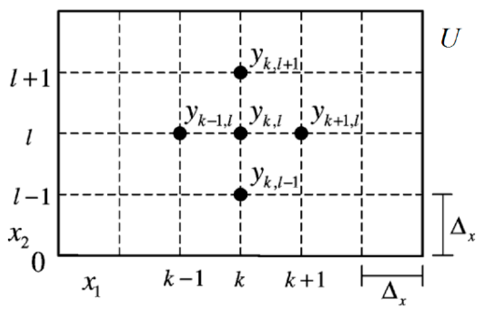
Consider a typical mesh grid as shown in Figure 1. The state variable is represented by at the grid node , where and , i.e., at the grid point , and the finite difference approximation scheme for the partial differential operator can be written as follows [14,16]:
.
Based on the finite difference approximation in Equation (28), the LPDS in Equation (1) can be represented by the following finite difference system:
.
Let us denote:
then we get:
For the simplification of entropy measurement for the LPDS in Equation (1), we will define a spatial state vector at all grid node in Figure 1. For the Dirichlet boundary conditions [16], the values of at the boundary are fixed. For example, , where . We have at or . Therefore, the spatial state vector for state variables at all grid nodes is defined as follows:
where . Note that is the dimension of the vector for each grid node and is the number of grid nodes. For example, let and , then we have . To simplify the index of the node in the spatial state vector , we will denote the symbol to replace . Note that the index is from 1 to N, i.e.:
where in Equation (32). Thus, the linear difference model of two indices in Equation (31) could be represented with only one index as follows:
where with and is defined as follows:
where and denote the zero matrix and identity matrix, respectively.
We will collect all states of the grid nodes given in Equation (33) to the spatial state vector given in Equation (32). The Kronecker product can be used to simplify the representation. Using the Kronecker product, the systems at all grid nodes given in Equation (33) can be represented by the following spatial state space system (i.e., the linear dynamic systems of Equation (33) at all grid points within domain in Figure 1 are represented by a spatial state space system [14]):
where , , and denotes the Kronecker product between and .
Definition 1. [17,36]: Let , . Then the Kronecker product of and is defined as the following matrix:
Remark 7. Since the spatial state vector in Equation (32) is used to represent at all grid points, in this situation, , , and in the measurement of system randomness in Equations (5) or (9) could be modified by the temporal forms , , and , respectively, for the spatial state space system in (35), where the Lyapunov function is related to the Lyapunov function as . Therefore, for the spatial state space system in Equation (35), the system randomness in Equations (5) or (9) is modified as follows:
or:
Hence, our entropy measurement problem of the LPDS in Equation (1) becomes the measurement of the entropy of the spatial state system Equation (35), as given below.
Proposition 3. For the linear spatial state space system in Equation (35), if the following Riccati-like inequality holds for a positive definite matrix :
or equivalently:
where , then the system randomness in Equations (36) or (37) of linear spatial state space system in Equation (35) has the upper bound .
Proof. The proof is similar to the proof of Corollary 1 in Appendix B and can be obtained by replacing , and with , and , respectively. ☐
Therefore, the randomness of the linear spatial state space system in Equation (35) can be obtained by solving the following LMI-constrained optimization problem:
Hence, the system entropy of the linear spatial state space system in Equation (33) can be calculated using .
Remark 8. (i) The Riccati-like inequality in Equation (38) or the LMI in Equation (39) is an approximation of the HJII in Equation (10) with the finite difference scheme given in Equation (28). If the finite difference, shown in Equation (28), , then in Equation (40) will approach in Equation (11). (ii) Substituting into Equation (38), we get:
If the eigenvalues of are more negative (more stable), the randomness as well as the entropy is smaller. Similarly, the LSPDS in Equation (18) can be approximated by the following stochastic spatial state space system via finite difference scheme [14]:
where , and the Hadamard product of matrices (or vectors) and of the same size is the entry-wise product denoted as .
Then we can get the following result.
Corollary 3. For the linear stochastic spatial state space system Equation (42), if the following Riccati-like inequality holds for a positive definite symmetric :
or equivalently, the following LMI has a positive definite symmetric solution :
then the system randomness of the stochastic state space system in Equation (42) has an upper bound , where .
Proof. The proof is similar to the proof of Corollary 2 in Appendix D. ☐
Therefore, the system randomness of the linear stochastic state space system Equation (42) can be obtained by solving the following LMI-constrained optimization problem:
and hence the system entropy of the stochastic spatial state space system in Equation (42) can be obtained using . Substituting into (43), we get:
Remark 9. Comparing Equation (41) with Equation (46), because of the term from the intrinsic random fluctuation, it can be seen that the LSPDS with random fluctuations will lead to a larger and a larger system entropy S. ☐
4. System Entropy Measurement of NSPDSs
Most partial dynamic systems are nonlinear; hence, the measurement of the system entropy of nonlinear partial differential systems (NPDSs) will be discussed in this section. Consider the following NPDSs in the domain :
where , and are the nonlinear functions with , , and , respectively. The nonlinear diffusion functions satisfy , and . If the equilibrium point of interest is not at the origin, for the convenience of analysis, the origin of the NPDS must be shifted to the equilibrium point (shifted to zero). The initial and boundary conditions are the same as the LPDS in Equation (1); then, we get the following result.
Proposition 4. For the NPDS in Equation (47), if the following HJII holds for a Lyapunov function with :
then the system randomness of the NPDS in Equation (47) has an upper bound as given in Equation (5).
Proof. See Appendix E. ☐
Based on the condition of upper bound given in Equation (48), the system randomness could be obtained by solving the following HJII-constrained optimization problem:
Hence, the system entropy of NPDS in Equation (47) can be obtained using . If the NPDS in Equation (47) is free of the diffusion operator as with the following conventional nonlinear dynamic system:
then the result of Proposition 4 is reduced to the following corollary.
Corollary 4. For the nonlinear dynamic system Equation (50), if the following HJII holds for a positive Lyapunov function with :
then the system randomness of the nonlinear dynamic system in Equation (50) has an upper bound
Proof. The proof is similar to that of Proposition 4 without consideration of the diffusion operator and spatial integration on the domain .
Hence, the system randomness of the nonlinear dynamic system in Equation (50) can be obtained by solving the following HJII-constrained optimization problem:
and the system entropy is obtained using . If the NPDS in Equation (47) suffers from random intrinsic fluctuations as with the NSPDSs:
where denotes the random intrinsic fluctuation, then the NSPDS in Equation (53) can be written in the following form:
Therefore, we can get the following result:
Proposition 5. For the NSPDS in Equations (53) or (54), if the following HJII holds for a Lyapunov function with :
then the system randomness of the NSPD S in Equations (53) or (54) can be obtained by solving the following HJII-constrained optimization problem:
Proof. See Appendix F. ☐
Remark 10. By comparing the HJII in Equation (48) with the HJII in Equation (55), due to the extra term from the random intrinsic fluctuation in Equation (53), it can be seen that the system randomness of the NSPDS in Equation (53) must be larger than the system randomness of the NPDS in Equation (47). Hence, the system entropy of the NSPDS in Equation (53) is larger than that of the NPDS in Equation (47).
5. System Entropy Measurement of NSPDS via Global Linearization and Semi-Discretization Finite Difference Scheme
In general, it is very difficult to solve the HJII in Equations (48) or (55) for the system entropy measurement of the NPDS in Equation (47) or the NSPDS in Equation (53), respectively. In this study, the global linearization technique and a finite difference scheme were employed to simplify the entropy measurement of the NPDS in Equation (47) and NSPDS in Equation (53). Consider the following global linearization of the NPDS in Equation (47), which is bounded by a polytope consisting of L vertices [12,37]:
where denotes the convex hull of a polytope with vertices defined in Equation (57). Then, the trajectories of for the NPDS in Equation (47) will belong to the convex combination of the state trajectories of the following linearized PDSs derived from the vertices of the polytope in Equation (57):
From the global linearization theory [16,37], if Equation (57) holds, then every trajectory of the NPDS in Equation (47) is a trajectory of a convex combination of linearized PDSs in Equation (58), and they can be represented by the convex combination of linearized PDSs in Equation (58) as follows:
where the interpolation functions are selected as and they satisfy and . That is, the trajectory of the NPDS in Equation (47) can be approximated by the trajectory of the interpolated local LPDS given in Equation (59).
Following the semi-discretization finite difference scheme in Equations (28)–(34), the spatial state space system of the interpolated PDS in Equation (59) can be represented as follows:
where and are defined in (35). That is, the NPDS in Equation (47) is interpolated through local linearized PDSs in Equation (59) to approximate the NPDS in Equation (47) using global linearization and semi-discretization finite difference scheme.
Remark 11. In fact, there are many interpolation schemes for approximating a nonlinear dynamic system with several local linear dynamic systems such as Equation (60); for example, fuzzy interpolation and cubic spline interpolation methods [13]. Then, we get the following result. ☐
Proposition 6. For the linear dynamic systems in Equation (60), if the following Riccati-like inequalities hold for a positive definite symmetric :
or equivalently:
where , , and are defined as , and , respectively, then the system randomness of the NPDSs in Equation (47) or the interpolated dynamic systems in Equation (60) have an upper bound .
Proof. See Appendix G. ☐
Therefore, the system randomness of the NPDSs in Equation (47) or the interpolated dynamic systems in Equation (60) can be obtained by solving the following LMIs-constrained optimization problem:
Hence, the system entropy of the NPDSs in Equation (47) or the interpolated dynamic systems in Equation (60) can be obtained using . By substituting into the Riccati-like inequalities in Equation (61), we can obtain:
Obviously, if the eigenvalues of local system matrices are more negative (more stable), the randomness is smaller and the corresponding system entropy is also smaller, and vice versa.
The NSPDs given in Equation (54) can be approximated using the following global linearization technique [12,37]:
Then, the NSPDs with the random intrinsic fluctuation given in Equation (53) can be approximated by the following interpolated spatial state space system [14]:
i.e., we could interpolate local interpolated stochastic spatial state space systems to approximate the NSPDs in Equation (53). Then, we get the following result.
Proposition 7. For the NSPDs in Equation (54) or the linear interpolated stochastic spatial state space systems in (66), if the following Riccati-like inequalities hold for a positive definite symmetric :
or equivalently:
where , then the system randomness of the NSPDs in Equation (53) or the interpolated stochastic systems in Equation (66) can be obtained by solving the following LMIs-constrained optimization problem:
Then, the system entropy of NSPD in Equation (53) or the interpolated stochastic systems in Equation (66) could be obtained as .
Proof. See Appendix H. ☐
Substituting into in Equation (67), we get:
Comparing (64) with Equation (70), of the NSPDS in Equation (53) is larger than of the NPDS in Equation (47), i.e., the random intrinsic fluctuation will increase the system entropy of the NSPDS. Based on the above analysis, the proposed system entropy measurement procedure of NSPDSs is given as follows:
- Step 1:
- Given the initial value of state variable, the number of finite difference grids, the vertices of the global linearization, and the boundary condition.
- Step 2:
- Construct the spatial state space system in Equation (60) by finite difference scheme.
- Step 3:
- Construct the interpolated state space system Equation (66) by global linearization method.
- Step 4:
- If the error between the original model Equation (54) and the approximated model Equation (66) is too large, we could adjust the density of grid nodes of finite difference scheme and the number of vertices of global linearization technique and return to Step 1.
- Step 5:
- Solve the eigenvalue problem in Equation (69) to obtain and , and then system entropy .
6. Computational Example
Based on the aforementioned analyses for the system entropy of the considered PDSs, two computational examples are given below for measuring the system entropy.
Example 1. Consider a heat transfer system in a 1m × 0.5m thin plate with a surrounding temperature of 0 °C as follows [38]:
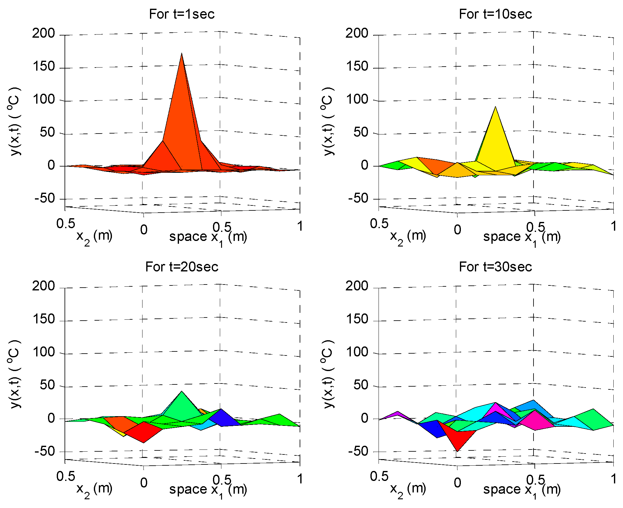
and y(x,t) = 0 °C, ∀ t, ∀ x on the boundary of U =[0,1]×[0,0.5]. Here, y(x,t) is the temperature function, location x is in meters, time t is in s, is the thermal diffusivity [4,5,6,7,9], and the term with denotes the thermal dissipation when the temperature of the plate is greater than the surrounding temperature, i.e., °C, or the thermal absorption when the temperature on the plate is less than the surrounding temperature, i.e., °C. The output coupling . is the environmental thermal fluctuation input with . We can estimate the system entropy of the heat transfer system in Equation (71). Based on Proposition 3 and the LMI-constrained optimization problem Equation (40), we can calculate the system entropy of the heat transfer system in Equation (71) as . In this calculation of the system entropy, the grid spacing of the finite difference scheme was chosen as 0.125m such that there are interior grid points and 24 boundary points in . The temperature distributions of the heat transfer system in Equation (71) at , 10, 30 and 50 s are shown in Figure 2 with . Due to the diffusion term , the heat temperature of transfer system Equation (71) will be uniformly distributed gradually. Even if the thin plate has initial value (heat source) or some other influences like input signal and intrinsic random fluctuation, the temperature of the thin plate will gradually achieve a uniform distribution to increase the system entropy. This phenomenon can be seen in Figure 2, Figure 3, Figure 4 and Figure 5.
Suppose that the heat transfer system in Equation (71) suffers from the following random intrinsic fluctuation:
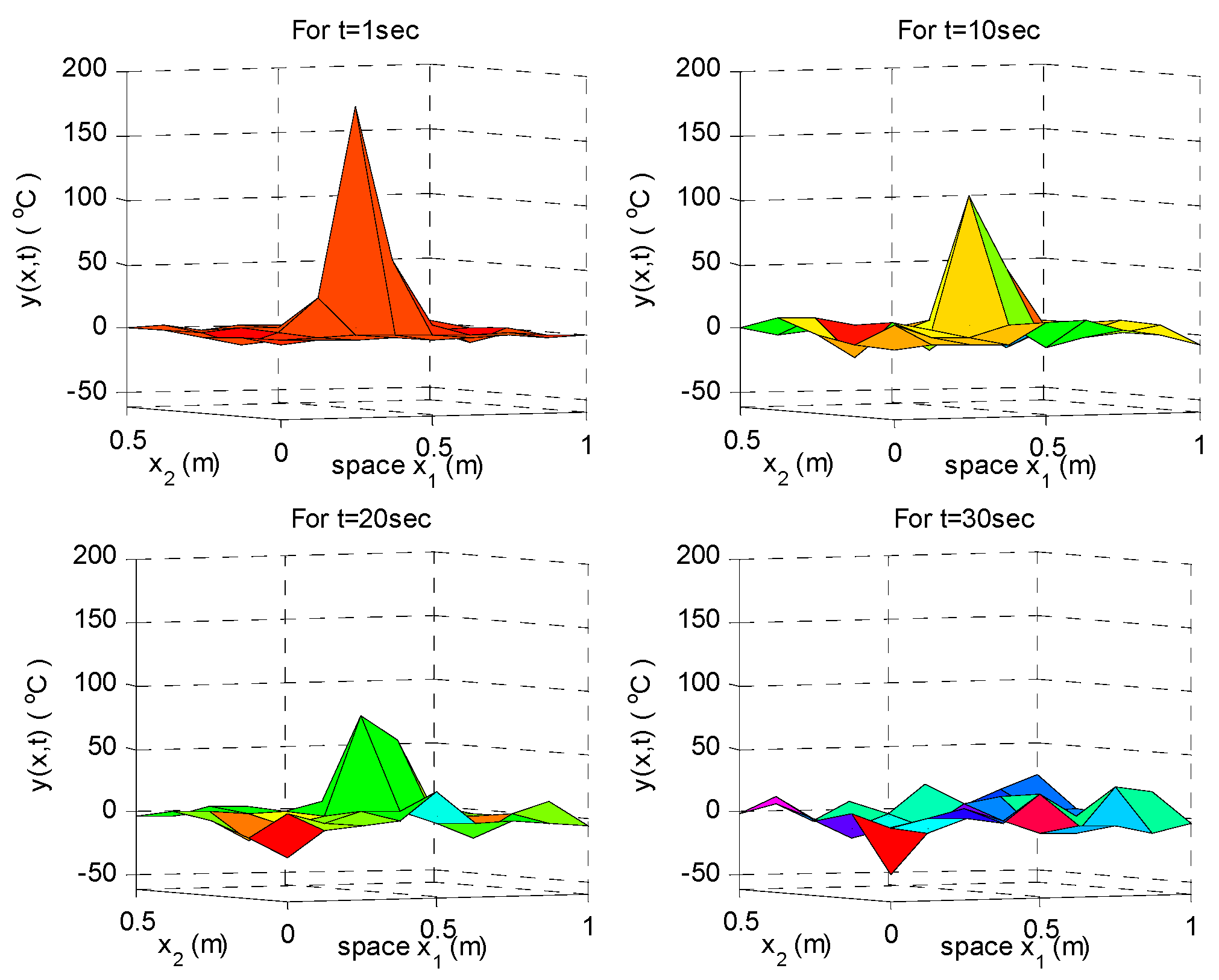
where the term with is due to the random parameter variation of the term . Then, the temperature distributions of the heat transfer system in Equation (72) at 1, 10, 30 and 50 s are shown in Figure 3. Based on the Corollary 3 and the LMI-constrained optimization problem in Equation (45), we can calculate the system entropy of the stochastic heat transfer system in Equation (72) as . Obviously, it can be seen that the system entropy of the stochastic heat transfer system in Equation (72) is larger than the heat transfer system in Equation (71) without intrinsic random fluctuation.
Example 2. A biochemical enzyme system is used to describe the concentration distribution of the substrate in a biomembrane. For the enzyme system, the thickness of the artificial biomembrane is 1 μm. The concentration of the substrate is uniformly distributed inside the artificial biomembrane. Since the biomembrane is immersed in the substrate solution, the reference axis is chosen to be perpendicular to the biomembrane. The biochemical system can be formulated as follows [13]:
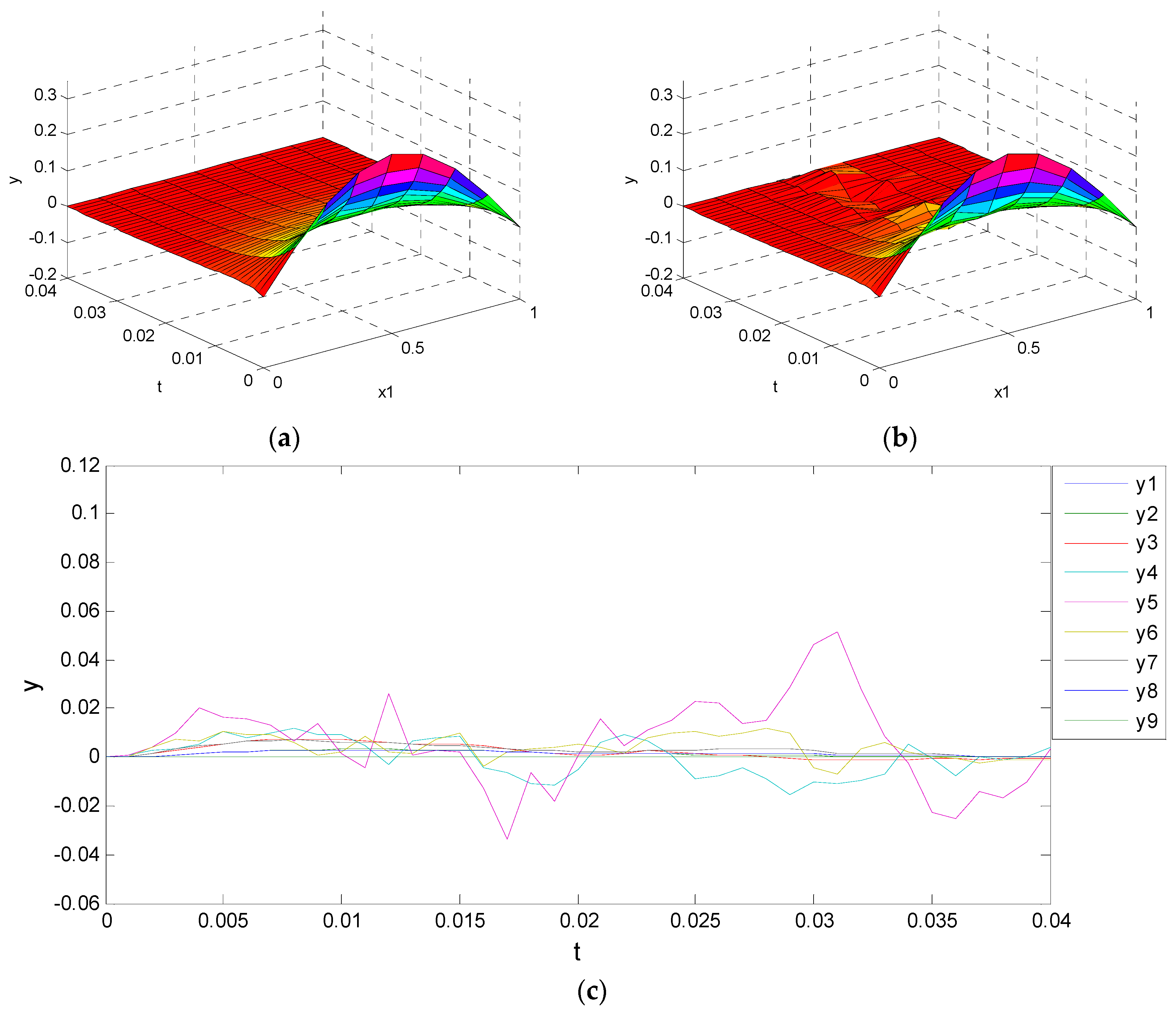
where is the concentration of the substrate in the biomembrane, is the substrate diffusion coefficient, is the maximum activity in one unit of the biomembrane, is the Michaelis constant, and is the substrate inhibition constant. The parameters of the biochemical enzyme system are given by , , , and the output coupling . Note that the equilibrium point in Example 2 is at zero. The concentration of the initial value of the substrate is given by . The boundary conditions used to restrict the concentration are zero at and , i.e., , . A more detailed discussion about the enzyme can be found in [13]. Suppose that the biochemical enzyme system is under the effect of an external signal . For the convenience of computation, the external signal is assumed as a zero mean Gaussian noise with a unit variance. The influence function of external signal is defined as at and (μm). Based on the global linearization in Equation (57), we get and , as shown in detail in Appendix I. The concentration distributions of the real system and approximated system are given in Figure 4 with , i.e., . Clearly, the approximated system based on the global linearization technique and finite difference scheme efficiently approach the nonlinear function. Based on Proposition 6 and the LMIs-constrained optimization given in Equation (63), we can obtain as shown in detail in Appendix J and calculate the system entropy of the enzyme system in Equation (73) as .
Therefore, it is clear that the approximated system in Equation (60) can efficiently approximate biochemical enzyme system in Equation (73). In this simulation, . Suppose that the biochemical system in Equation (73) suffers from the following random intrinsic fluctuation:
where the term with is the random parameter variation from the term . Based on the global linearization in Equation (65), we can get as shown in detail in Appendix K. Based on the Proposition 7 and the LMIs-constrained optimization given in Equation (69), we can solve as shown in detail in Appendix L and calculate the system entropy of the enzyme system in Equation (74) as .
Clearly, because of the intrinsic random parameter fluctuation, the system entropy of the stochastic enzyme system given in Equation (74) is larger than that of the enzyme system given in Equation (73).
The computation complexities of the proposed LMI-based indirect entropy measurement method is about in solving LMIs, where is the dimension of , is the number of global interpolation points. We also calculate the elapsed time of the simulations examples by using MATLAB. The computation times including the drawing of the corresponding figures to solve the LMI constrained optimization problem are given as follows: in Example 1, the case of heat transfer system in Equation (71) is 183.9 s; the case of heat transfer system with random fluctuation in Equation (72) is 184.6 s. In Example 2, the case of biochemical system in Equation (73) is 17.7 s, the case of biochemical system with random fluctuation in Equation (74) is 18.6 s. The RAM of the computer is 4.00 GB, the CPU we used is AMD A4-5000 CPU with Radeon(TM) HD Graphics, 1.50 GHz. The results are reasonable. Because the dimension of grid nodes in Example 1 is and the dimension of grid nodes in Example 2 is , obviously, the computation time in Example 1 is much larger than in Example 2. Further, the time spent of the system without the random fluctuation is slightly faster than the system with the random fluctuation. The conventional algorithms of calculating entropy have been applied in image processing, digital signal processing, and particle filters, like in [39,40,41]. The conventional algorithms for calculating entropy just can be used in linear discrete systems, but in fact many systems are nonlinear and continuous. The indirect entropy measurement method we proposed can deal with the nonlinear stochastic continuous systems. Though the study in [24] is about the continuous nonlinear stochastic system, many physical systems are always modeled using stochastic partial differential dynamic equation in the spatio-temporal domain. The indirect entropy measurement method we proposed can be employed to solve the system entropy measurement in nonlinear stochastic partial differential system problem.
7. Conclusions
In this study, the system entropy of stochastic partial differential systems (SPDSs) was introduced as the difference between input signal entropy and output signal entropy and was found to be the logarithm of the output signal randomness-to-input signal randomness ratio. We found that the system stability was inversely related to the system entropy and that intrinsic random fluctuation could increase the system entropy. If the eigenvalues of the system matrices are further in the left-hand side of the s-complex domain, then the SPDS has lower system entropy, and vice versa. If the output and the input signal randomness values are equal and the system is independent of the initial value, then the system entropy is zero. To estimate the system entropy of nonlinear stochastic partial differential systems (NSPDSs), the global linearization technique and finite difference scheme were employed to represent the NSPDS using the spatial state space system given in Equation (66). Therefore, the system entropy measurement problem of NPDSs became the problem of solving the HJII-constrained optimization problem given in Equation (55), which can be replaced by a simple LMIs-constrained optimization problem given in Equation (69). Hence, using the LMI-toolbox of MATLAB, we could easily calculated the system entropy of NSPDS. Finally, two examples were provided to illustrate the measurement procedure of the system entropy and to confirm that the PDSs with intrinsic random fluctuation possess greater system entropy.
Acknowledgments
This work was supported by National Science Council under contract No. MOST-104-2221-E-007-124-MY3.
Author Contributions
Bor-Sen Chen: Methodology development, conception and design, data interpretation and improved the scientific quality of the manuscript. Chao-Yi Hsieh: Manuscript writing, computational simulation and interpretation. Shih-Ju Ho: Simulation assistance, conception and design and data interpretation. All authors have read and approved the final manuscript.
Conflicts of Interest
The authors declare no conflict of interest.
Appendixes
Lemma 1. [12]: For any matrices (or vectors) , and a symmetric matrix with appropriate dimensions, we have:
for any positive constant . ☐
Lemma 2. [42]: Let be any matrix with appropriate dimension and be the interpolation function for the th local system and . Then, we have:
With Lemma 2, the LMI-constrained optimization in Equations (62) or (68) can be solved efficiently. ☐
Appendix A.
Proof of Proposition 1.
From the fact that , we have:
From Lemma 1:
Substituting Equation (A3) into Equation (A2), we get:
If the HJII in given Equation (10) holds, then the system randomness in Equation (9) holds. If and , then the HJII in Equation (10) will lead to the inequality in Equation (5). ☐
Appendix B.
Proof of Corollary 1
In the conventional linear dynamic system in Equation (12), which is independent on , the HJII in Equation (10) for the system randomness to have an upper bound becomes the following inequality:
If we choose the Lyapunov function as , then the HJII for the existence of the upper bound in (B1) becomes:
or:
Therefore, if the Riccati-like inequality in Equation (14) holds, then the inequality in Equation (B3) also holds and the system randomness of the linear dynamic system in Equation (12) has an upper bound
. ☐
Appendix C.
Proof of Proposition 2
In this situation, we will follow the proof procedure in Appendix A:
From the fact that and , substituting Equation (C1) into Equation (C2), we get:
By using the inequality Equation (A3), we get:
Therefore, if the HJII given in Equation (20) holds, then the inequality of system randomness in Equation (9) holds. If the initial condition , then , and the inequality of the system randomness in Equation (5) holds. ☐
Appendix D.
Proof of Corollary 2
For the linear stochastic system in Equation (22), the HJII in Equation (20) for with an upper bound becomes:
If we choose the Lyapunov function as , then the condition Equation (D1) for with an upper bound becomes:
Therefore, if the Riccati-like inequality in Equation (24) holds, then the system randomness has an upper bound . ☐
Appendix E.
Proof of Proposition 4.
From the fact that
From Lemma 1:
Substituting Equation (E3) into Equation (E2), we get:
If the HJII in Equation (48) holds, then has an upper bound as shown in Equation (9). If , then , and the HJII in Equation (48) and Equation (E4) will lead to Equation (5). ☐
Appendix F.
Proof of Proposition 5
For the NPDS given in Equation (54), by using the formula, we get:
From the fact that and by following a similar procedure explained in Appendix E, we get:
If the HJII in Equation (55) holds, then the system randomness of the NSPDSs in Equations (53) or (54) has an upper bound as Equation (5) or Equation (9). ☐
Appendix G.
Proof of Proposition 6.
From the fact of the following inequality:
from Lemma 2, and the choice of , we get:
If the inequalities in Equations (61) or (62) holds, then we get Equation (36) if or Equation (37) if ; i.e., has an upper bound as shown in Equations (36) or (37). ☐
Appendix H.
Proof for Proposition 7.
From the fact that , , Equation (G2), Lemma 2, and the choice of , we get:
From the Riccati-like inequalities in Equation (67), we get Equation (36) if or Equation (37) if . Then, we can find that has an upper bound given in Equations (36) or (37). ☐
Appendix I. The Values of the Matrices , and in Example 2
Appendix J. The Values of the Matrix in Example 2 without the Random Fluctuation
Appendix K. The Values of the Matrices is in Example 2
Appendix L. The Value of the Matrix is in Example 2 with the Random Fluctuation
References
- Golan, A.; Judge, G.G.; Miller, D. Maximum Entropy Econometrics: Robust Estimation with Limited Data; Wiley: New York, NY, USA, 1996. [Google Scholar]
- Golan, A. Information and entropy econometrics—Volume overview and synthesis. J. Econ. 2007, 138, 379–387. [Google Scholar]
- Racine, J.S.; Maasoumi, E. A versatile and robust metric entropy test of time-reversibility, and other hypotheses. J. Econ. 2007, 138, 547–567. [Google Scholar] [CrossRef]
- Ruiz, M.D.; Guillamon, A.; Gabaldon, A. A new approach to measure volatility in energy markets. Entropy 2012, 14, 74–91. [Google Scholar] [CrossRef]
- Lebiedz, D. Entropy-related extremum principles for model reduction of dissipative dynamical systems. Entropy 2010, 12, 706–719. [Google Scholar] [CrossRef]
- Gupta, M.; Srivastava, S. Parametric bayesian estimation of differential entropy and relative entropy. Entropy 2010, 12, 818–843. [Google Scholar] [CrossRef]
- Popkov, Y.S. New class of multiplicative algorithms for solving of entropy-linear programs. Eur. J. Oper. Res. 2006, 174, 1368–1379. [Google Scholar] [CrossRef]
- Powell, G.; Percival, I. A spectral entropy method for distinguishing regular and irregular motion of hamiltonian systems. J. Phys. A Math. General 1979, 12. [Google Scholar] [CrossRef]
- Popkov, Y.; Popkov, A. New methods of entropy-robust estimation for randomized models under limited data. Entropy 2014, 16, 675–698. [Google Scholar] [CrossRef]
- Chen, B.; Yan, Z.L.; Chen, W. Defect detection for wheel-bearings with time-spectral kurtosis and entropy. Entropy 2014, 16, 607–626. [Google Scholar] [CrossRef]
- Yan, R.Q.; Gao, R.X. Approximate entropy as a diagnostic tool for machine health monitoring. Mech. Syst. Signal Process. 2007, 21, 824–839. [Google Scholar] [CrossRef]
- Boyd, S.P. Linear Matrix Inequalities in System and Control Theory; Society for Industrial and Applied Mathematics: Philadelphia, PA, USA, 1994. [Google Scholar]
- Chen, B.S.; Chang, Y.T. Fuzzy state-space modeling and robust observer-based control design for nonlinear partial differential systems. IEEE Trans. Fuzzy Syst. 2009, 17, 1025–1043. [Google Scholar] [CrossRef]
- Chen, W.H.; Chen, B.S. Robust stabilization design for stochastic partial differential systems under spatio-temporal disturbances and sensor measurement noises. IEEE Trans. Circuits Syst. I Regular Papers 2013, 60, 1013–1026. [Google Scholar] [CrossRef]
- Chow, P.L. Stochastic Partial Differential Equations; Chapman & Hall/CRC: Boca Raton, FL, USA, 2007. [Google Scholar]
- Pao, C.V. Nonlinear Parabolic and Elliptic Equations; Plenum Press: New York, NY, USA, 1992. [Google Scholar]
- Chen, B.-S.; Chen, W.-H.; Zhang, W. Robust filter for nonlinear stochastic partial differential systems in sensor signal processing: Fuzzy approach. IEEE Trans. Fuzzy Syst. 2012, 20, 957–970. [Google Scholar] [CrossRef]
- Lucia, U. Thermodynamic paths and stochastic order in open systems. Phys. A Stat. Mech. Appl. 2013, 392, 3912–3919. [Google Scholar] [CrossRef]
- Lucia, U.; Ponzetto, A.; Deisboeck, T.S. A thermodynamic approach to the ‘mitosis/apoptosis’ ratio in cancer. Phys. A Stat. Mech. Appl. 2015, 436, 246–255. [Google Scholar] [CrossRef]
- Lucia, U. Irreversible entropy variation and the problem of the trend to equilibrium. Phys. A Stat. Mech. Appl. 2007, 376, 289–292. [Google Scholar] [CrossRef]
- Lucia, U. Maximum entropy generation and κ-exponential model. Phys. A Stat. Mech. Appl. 2010, 389, 4558–4563. [Google Scholar] [CrossRef]
- Lucia, U. Irreversibility, entropy and incomplete information. Phys. A Stat. Mech. Appl. 2009, 388, 4025–4033. [Google Scholar] [CrossRef]
- Lucia, U. The gouy-stodola theorem in bioenergetic analysis of living systems (irreversibility in bioenergetics of living systems). Energies 2014, 7, 5717–5739. [Google Scholar] [CrossRef]
- Chen, B.-S.; Wong, S.-W.; Li, C.-W. On the calculation of system entropy in nonlinear stochastic biological networks. Entropy 2015, 17, 6801–6833. [Google Scholar] [CrossRef]
- Chang, W.; Wang, W.J. H∞ fuzzy control synthesis for a large-scale system with a reduced number of LMIs. IEEE Trans. Fuzzy Syst. 2015, 23, 1197–1210. [Google Scholar] [CrossRef]
- Lin, W.-W.; Wang, W.-J.; Yang, S.-H. A novel stabilization criterion for large-scale T-S fuzzy systems. IEEE Trans. Syst. Man Cybern. Part B Cybern. 2007, 37, 1074–1079. [Google Scholar] [CrossRef]
- Hsiao, F.-H.; Hwang, J.-D. Stability analysis of fuzzy large-scale systems. IEEE Trans. Syst. Man Cybern. Part B Cybern. 2001, 32, 122–126. [Google Scholar] [CrossRef] [PubMed]
- Wang, W.-J.; Luoh, L. Stability and stabilization of fuzzy large-scale systems. IEEE Trans. Fuzzy Syst. 2004, 12, 309–315. [Google Scholar] [CrossRef]
- Chen, C.-W.; Chiang, W.; Hsiao, F. Stability analysis of T–S fuzzy models for nonlinear multiple time-delay interconnected systems. Math. Comput. Simul. 2004, 66, 523–537. [Google Scholar] [CrossRef]
- Saat, S.; Nguang, S.K. Nonlinear H∞ output feedback control with integrator for polynomial discrete-time systems. Int. J. Robust Nonlinear Control 2013, 25, 1051–1065. [Google Scholar] [CrossRef]
- Saat, S.; Nguang, S.K.; Darsono, A.; Azman, N. Nonlinear H∞ feedback control with integrator for polynomial discrete-time systems. J. Frankl. Inst. 2014, 351, 4023–4038. [Google Scholar] [CrossRef]
- Chae, S.; Nguang, S.K. SOS based robust fuzzy dynamic output feedback control of nonlinear networked control systems. IEEE Trans. Cybern. 2014, 44, 1204–1213. [Google Scholar] [CrossRef] [PubMed]
- Johansson, R. System Modeling & Identification; Prentice Hall: Upper Saddle River, NJ, USA, 1993. [Google Scholar]
- Zhang, W.H.; Chen, B.S. State feedback H∞ control for a class of nonlinear stochastic systems. Siam J. Control Optim. 2006, 44, 1973–1991. [Google Scholar] [CrossRef]
- Zhang, W.H.; Chen, B.S.; Tseng, C.S. Robust H∞ filtering for nonlinear stochastic systems. IEEE Trans. Signal Process. 2005, 53, 589–598. [Google Scholar] [CrossRef]
- Laub, A.J. Matrix Analysis for Scientists and Engineers; SIAM: Philadelphia, PA, USA, 2005. [Google Scholar]
- Chen, B.S.; Chen, W.H.; Wu, H.L. Robust H2/H∞ global linearization filter design for nonlinear stochastic systems. IEEE Trans. Circuits Syst. I Regular Papers 2009, 56, 1441–1454. [Google Scholar] [CrossRef]
- Incropera, F.P.; DeWitt, D.P. Introduction to Heat Transfer, 3rd ed.; Wiley: New York, NY, USA, 1996. [Google Scholar]
- Nemcsics, Á.; Nagy, S.; Mojze, I.; Turmezei, P. Fractal and Structural Entropy Calculations on the Epitaxially Grown Fulleren Structures with the Help of Image Processing. In Proceedings of the 7th International Symposium on Intelligent Systems and Informatics, 2009 (SISY'09), Subotica, Serbia, 25–26 September 2009; pp. 65–67.
- Orguner, U. Entropy Calculation in Particle Filters. In Proceedings of the IEEE 17th Signal Processing and Communications Applications Conference, 2009 (SIU 2009), Antalya, Turkey, 9–11 April 2009; pp. 628–631.
- Voronych, A.; Pastukh, T. Methods of Digital Signal Processing Based on Calculation of Entropy Technologies. In Proceedings of the 2015 13th International Conference Experience of Designing and Application of CAD Systems in Microelectronics (CADSM), Lviv, Ukraine, 24–27 February 2015; pp. 379–381.
- Chen, B.-S.; Wu, C.-F. Robust scheduling filter design for a class of nonlinear stochastic poisson signal systems. IEEE Trans. Signal Process. 2015, 63, 6245–6257. [Google Scholar] [CrossRef]
Figure 1.
Finite difference grids on the spatio-domain .

Figure 2.
The temperature distribution of the heat transfer system given in Equation (71) at 1, 10, 30 and 50 s. Due to the diffusion term , the temperature of heat system will be uniformly distributed gradually to increase the system entropy.
Figure 2.
The temperature distribution of the heat transfer system given in Equation (71) at 1, 10, 30 and 50 s. Due to the diffusion term , the temperature of heat system will be uniformly distributed gradually to increase the system entropy.

Figure 3.
The temperature distribution of heat transfer system in Equation (72) at 1, 10, 30 and 50 s. Obviously, the temperature distribution of stochastic heat transfer system in Equation (72) is with more random fluctuations and with more system entropy than the heat transfer system in Equation (71). The temperature distribution is also uniformly distributed gradually to increase the system entropy as time goes on. In general, the temperature in Figure 3 is more random than Figure 2, i.e., with more system randomness and entropy.

Figure 4.
(a) Spatial-time profiles of the real biochemical system in Equation (73); (b) Spatial-time profiles of the approximated system in Equation (60) based on the finite difference scheme and global linearization technique; (c) The error between the real biochemical system in Equation (73) and the approximated system in Equation (60). Obviously, the approximated system based on finite difference scheme and global linearization method can approximate the biochemical enzyme system quite well.

Figure 5.
(a) Spatial-time profiles of the real biochemical system in Equation (74); (b) Spatial-time profiles of the approximated system in Equation (66) based on the finite difference scheme and global linearization technique; (c) The error between the real biochemical system in Equation (74) and the approximated system in Equation (66). Obviously, the approximated system in Equation (66) could approximate the real system in Equation (74) quite well.

© 2016 by the authors; licensee MDPI, Basel, Switzerland. This article is an open access article distributed under the terms and conditions of the Creative Commons by Attribution (CC-BY) license (http://creativecommons.org/licenses/by/4.0/).
Share and Cite
MDPI and ACS Style
Chen, B.-S.; Hsieh, C.-Y.; Ho, S.-J. System Entropy Measurement of Stochastic Partial Differential Systems. Entropy 2016, 18, 99. https://doi.org/10.3390/e18030099
AMA Style
Chen B-S, Hsieh C-Y, Ho S-J. System Entropy Measurement of Stochastic Partial Differential Systems. Entropy. 2016; 18(3):99. https://doi.org/10.3390/e18030099
Chicago/Turabian StyleChen, Bor-Sen, Chao-Yi Hsieh, and Shih-Ju Ho. 2016. "System Entropy Measurement of Stochastic Partial Differential Systems" Entropy 18, no. 3: 99. https://doi.org/10.3390/e18030099
Note that from the first issue of 2016, this journal uses article numbers instead of page numbers. See further details here.