
Mapping US Urban Extents from MODIS Data Using One-Class Classification Method


Abstract
:
1. Introduction
2. Data and Method
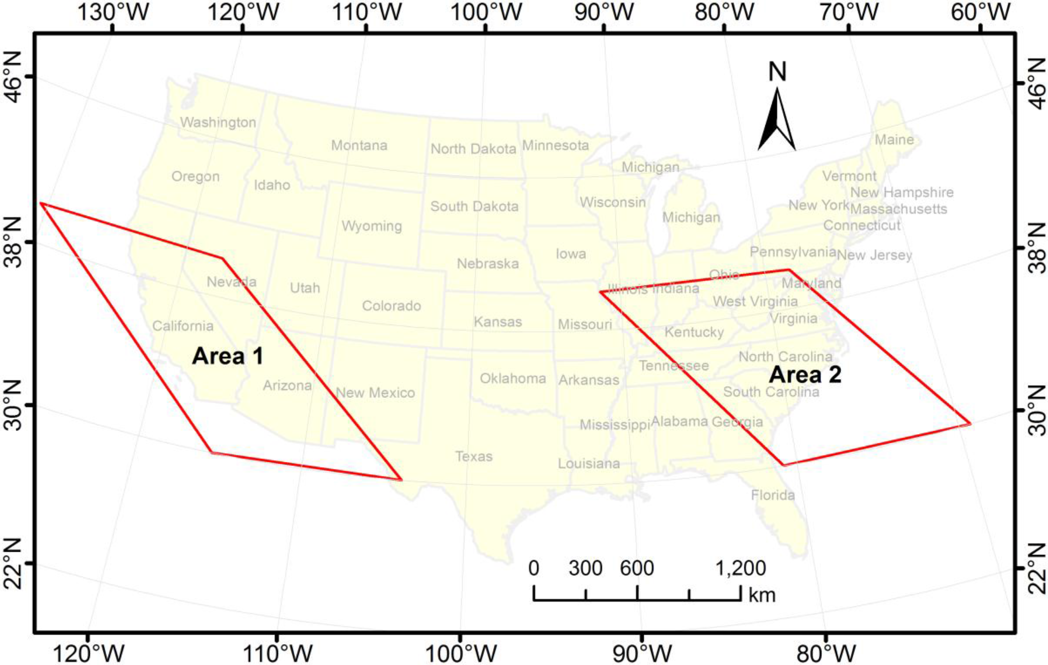
2.1. Urban Extent
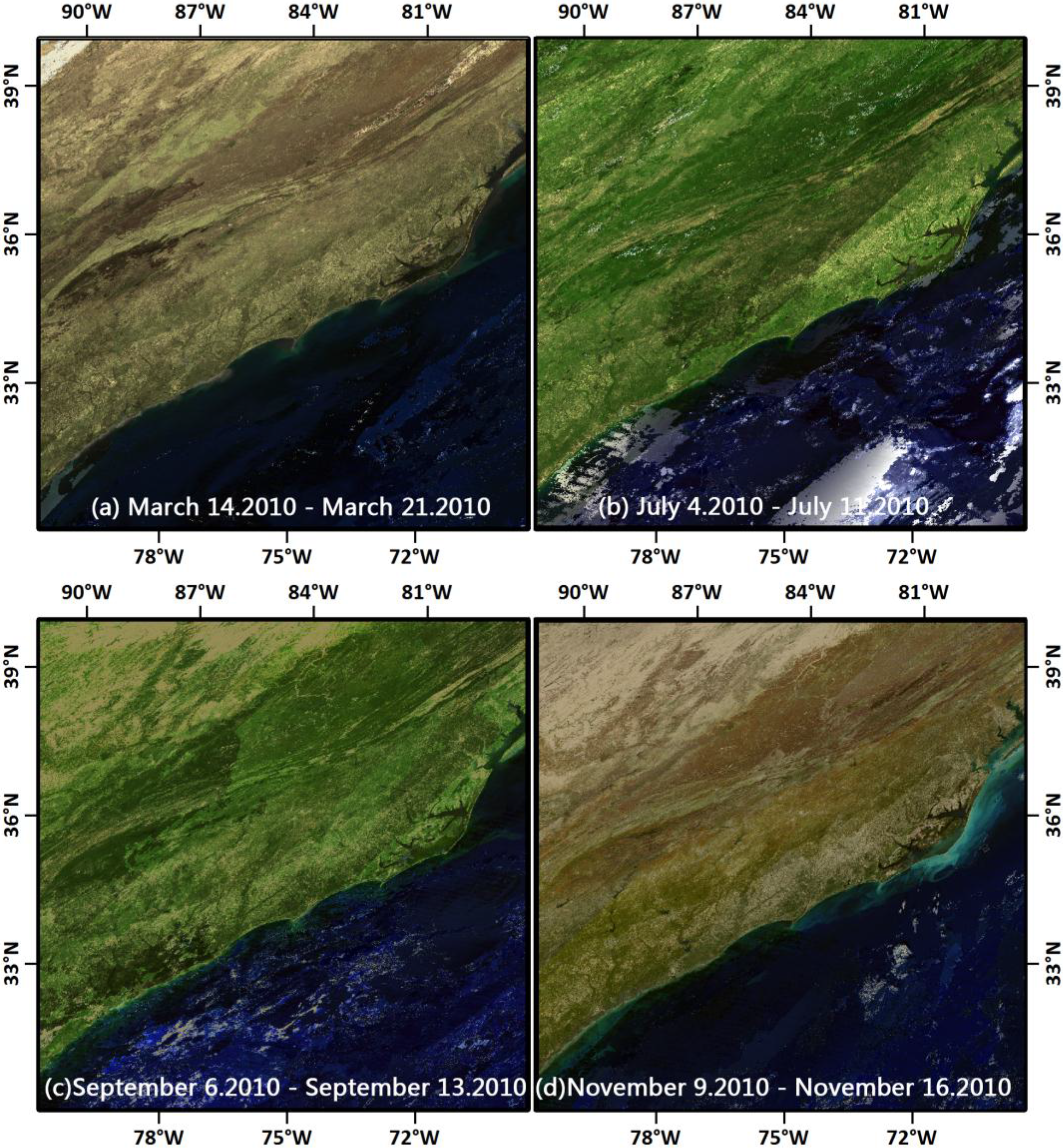
2.2. Dataset


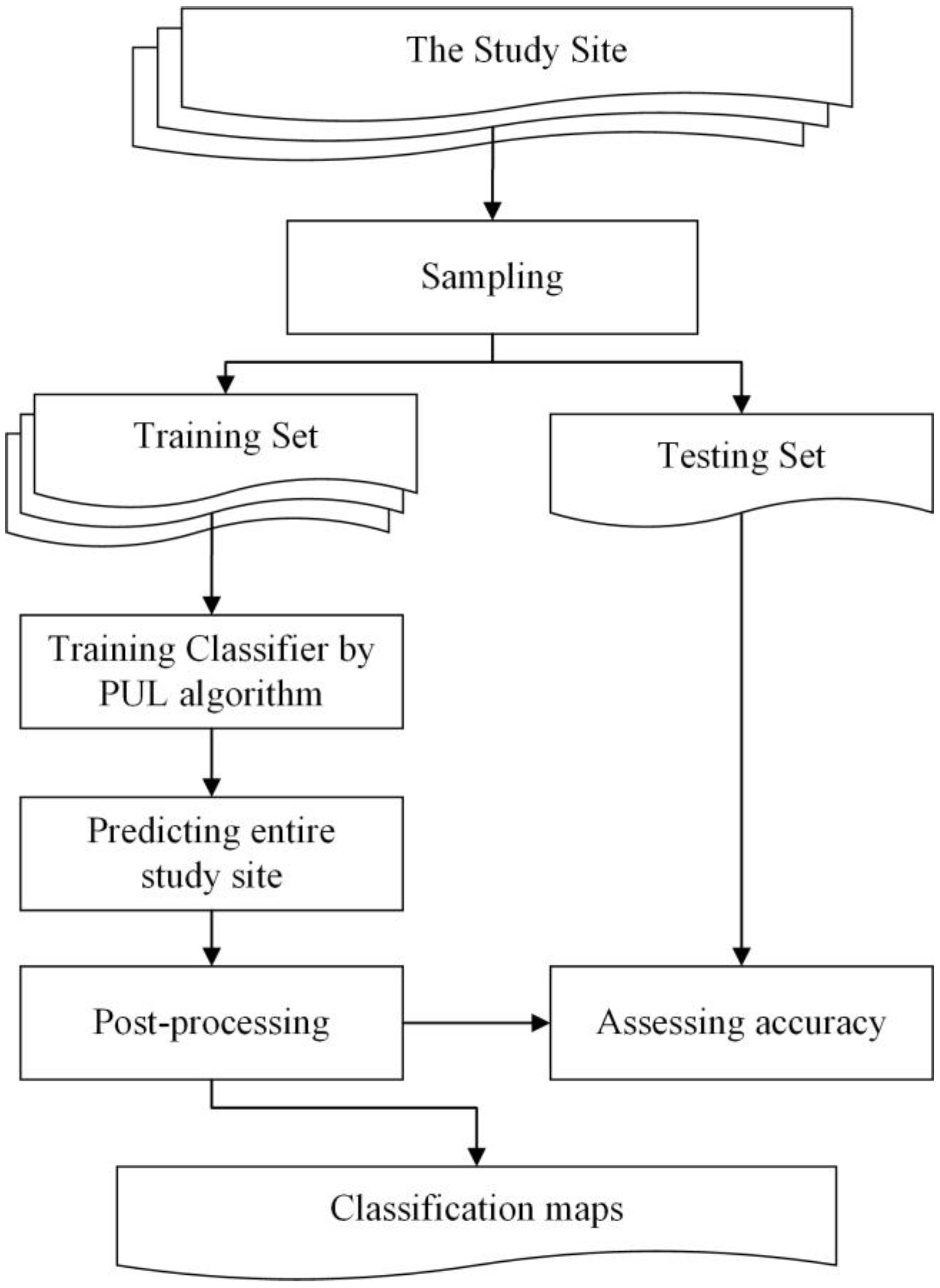
2.3. Method

2.3.1. Sampling

2.3.2. PUL
2.3.3. Post-Processing
2.4. Accuracy Assessment
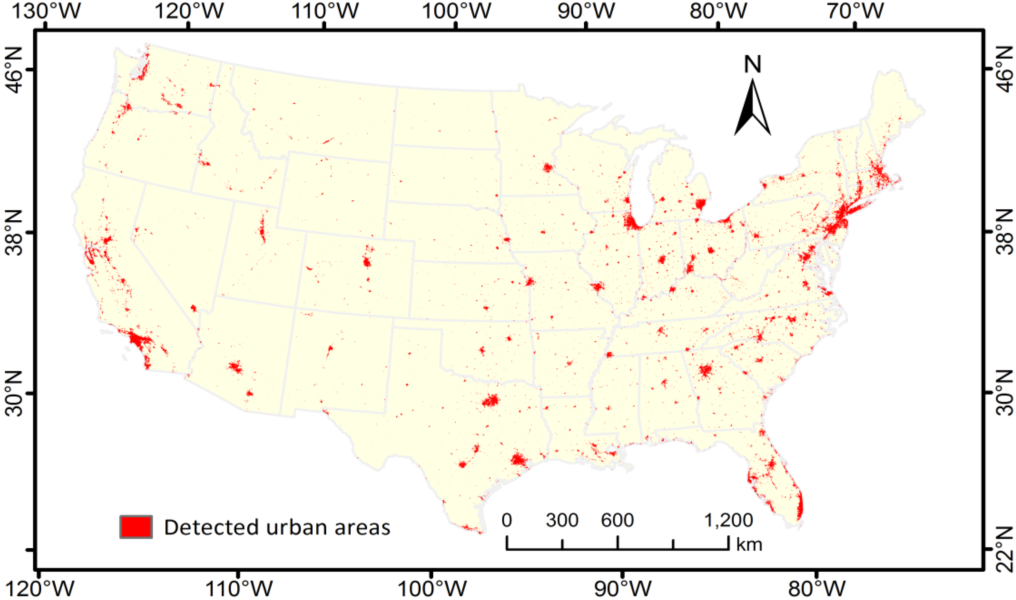
3. Results


| Reference data | Kappa Coefficient | ||||
|---|---|---|---|---|---|
| Non-urban | Urban | Total | User’s Accuracy (%) | ||
| Classified Data | |||||
| Non-urban | 10,912 | 1130 | 12,042 | 90.61 | |
| Urban | 288 | 7670 | 7958 | 96.38 | |
| Total | 11,200 | 8800 | 20,000 | ||
| 0.8546 | |||||
| Producer’s accuracy | 97.42% | 87.15% | 92.91% (Overall map accuracy) | ||
| City Size by Population * | Reference Number | Predicted Number | Omission Rate (%) |
|---|---|---|---|
| Large | 1 | 1 | 0 |
| Medium | 7 | 7 | 0 |
| Medium–small | 28 | 28 | 0 |
| Small | 240 | 240 | 0 |
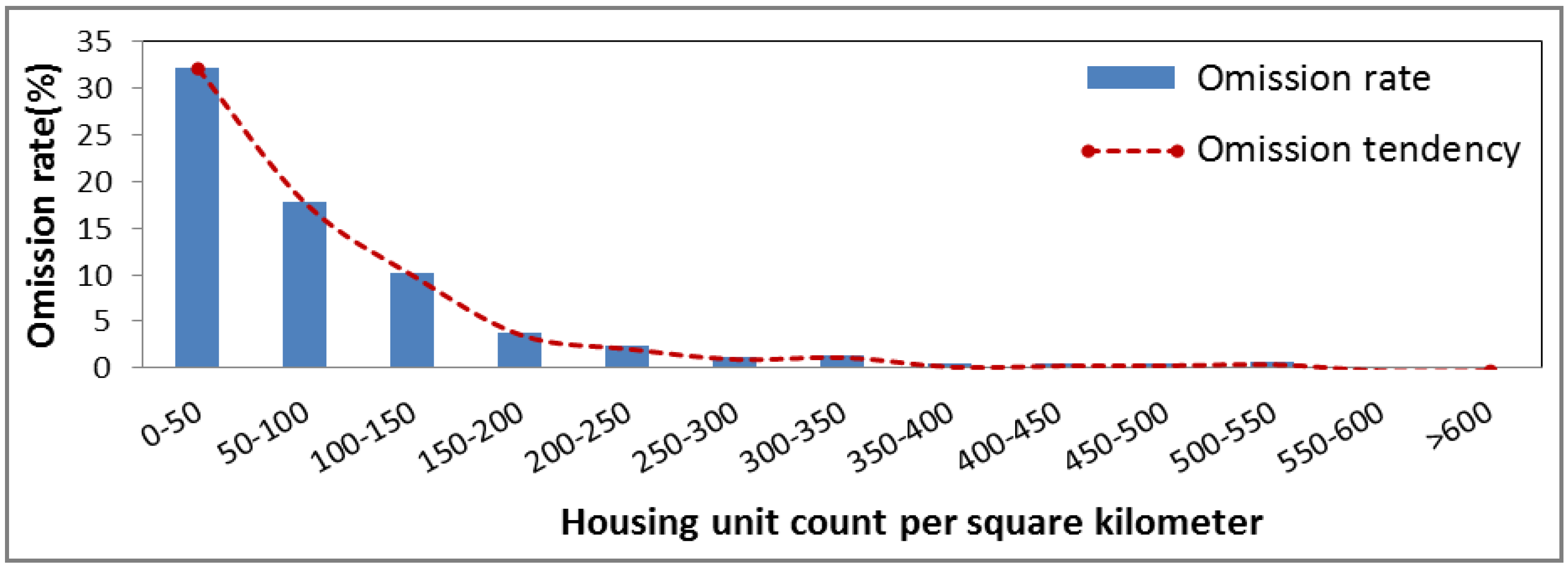
| Very small | 3197 | 3115 | 2.56 |
| Total | 3473 | 3391 | 2.36 |
| City Size by Population (million) | Reference Number | Predicted Number | Omission Rate (%) |
|---|---|---|---|
| 0.08–0.1 | 118 | 118 | 0 |
| 0.06–0.08 | 193 | 193 | 0 |
| 0.04–0.06 | 355 | 352 | 0.85 |
| 0.02–0.04 | 983 | 962 | 2.14 |
| 0.01–0.02 | 1,548 | 1,490 | 3.75 |
| Total | 3,197 | 3,115 | 2.56 |

4. Discussion
4.1. Urban Range Detection

4.2. Multi-Temporal Data
| User’s Accuracy (%) | Producer’s Accuracy (%) | Overall Accuracy (%) | Kappa Coefficient | |
|---|---|---|---|---|
| Single | 97.04 | 78.82 | 88.20 | 0.775 |
| Double | 98.08 | 81.60 | 90.00 | 0.800 |
| Quadruple | 98.14 | 84.50 | 91.45 | 0.829 |

4.3. Map Calibration with DMSP-OLS Data

5. Conclusions
Acknowledgements
Author Contritutions
Conflicts of Interest
References
- Mills, G. Cities as agents of global change. Int. J. Climatol. 2007, 27, 1849–1857. [Google Scholar]
- Foley, J.A.; DeFries, R.; Asner, G.P.; Barford, C.; Bonan, G.; Carpenter, S.R.; Chapin, F.S.; Coe, M.T.; Daily, G.C.; Gibbs, H.K.; et al. Global consequences of land use. Science 2005, 309, 570–574. [Google Scholar]
- Friedl, M.A.; Sulla-Menashe, D.; Tan, B.; Schneider, A.; Ramankutty, N.; Sibley, A.; Huang, X. MODIS Collection 5 global land cover: Algorithm refinements and characterization of new datasets. Remote Sens. Environ. 2010, 114, 168–182. [Google Scholar]
- Grimm, N.B.; Faeth, S.H.; Golubiewski, N.E.; Redman, C.L.; Wu, J.G.; Bai, X.M.; Briggs, J.M. Global change and the ecology of cities. Science 2008, 319, 756–760. [Google Scholar]
- Wu, J.G. Urban ecology and sustainability: The state-of-the-science and future directions. Landsc. Urban Plan. 2014, 125, 209–221. [Google Scholar]
- Cai, S.S.; Liu, D.S.; Sulla-Menashe, D.; Friedl, M.A. Enhancing MODIS land cover product with a spatial-temporal modeling algorithm. Remote Sens. Environ. 2014, 147, 243–255. [Google Scholar]
- Gong, P.; Wang, J.; Yu, L.; Zhao, Y.C.; Zhao, Y.Y.; Liang, L.; Niu, Z.; Huang, X.; Fu, H.; Liu, S.; et al. Finer resolution observation and monitoring of global land cover: First mapping results with Landsat TM and ETM+ data. Int. J. Remote Sens. 2013, 34, 2607–2654. [Google Scholar]
- Schneider, A.; Friedl, M.A.; Potere, D. Mapping global urban areas using MODIS 500-m data: New methods and datasets based on “urban ecoregions”. Remote Sens. Environ. 2010, 114, 1733–1746. [Google Scholar]
- Loveland, T.R.; Reed, B.C.; Brown, J.F.; Ohlen, D.O.; Zhu, Z.; Yang, L.; Merchant, J.W. Development of a global land cover characteristics database and IGBP DISCover from 1 km AVHRR data. Int. J. Remote Sens. 2000, 21, 1303–1330. [Google Scholar]
- Bartholome, E.; Belward, A.S. GLC2000: A new approach to global land cover mapping from Earth observation data. Int. J. Remote Sens. 2005, 26, 1959–1977. [Google Scholar]
- Arino, O.; Gross, D.; Ranera, F.; Leroy, M.; Bicheron, P.; Brockman, C.; Latham, J.; di Gregorio, A.; Brockman, C.; Witt, R.; et al. GlobCover: ESA service for global land cover from MERIS. In Proceedings of the IEEE International Geoscience and Remote Sensing Symposium, 2007, Barcelona, Spain, 23–28 July 2007.
- Bontemps, S.; Defourny, P.; Bogaert, E.V.; Arino, O.; Kalogirou, V.; Rerez, J.E. GLOBCOVER 2009—Products Description and Validation Reports. 2011. Available online: http://ionia1.esrin.esa.int/docs/GLOBCOVER2009_Validation_Report_2.2.pdf (accessed on 14 May 2015).
- CIESIN, Center for International Earth Science Information Network. Global Rural-Urban Mapping Project (GRUMP), Alpha Version: Urban Extents. 2004. Available online: http://sedac.ciesin.columbia.edu/gpw (accessed on 1 August 2009).
- Schneider, A.; Friedl, M.A.; Potere, D. A new map of global urban extent from MODIS satellite data. Environ. Res. Lett. 2009, 4. [Google Scholar] [CrossRef]
- Schneider, A.; Friedl, M.A.; Mciver, D.K.; Woodcock, C.E. Mapping urban areas by fusing multiple sources of coarse resolution remotely sensed data. Photogramm. Eng. Remote Sens. 2003, 69, 1377–1386. [Google Scholar]
- Yu, L.; Wang, J.; Li, X.C.; Li, C.C.; Zhao, Y.Y.; Gong, P. A multi-resolution global land cover dataset through multisource data aggregation. Sci. China: Earth Sci. 2014. [Google Scholar] [CrossRef]
- Vogelmann, J.E.; Howard, S.M.; Yang, L.; Larson, C.R.; Wylie, B.K.; van Driel, J.N. Completion of the 1990’s national land cover data set for the conterminous United States. Photogramm. Eng. Remote Sens. 2001, 67, 650–662. [Google Scholar]
- Fry, J.; Xian, G.; Jin, S.; Dewitz, J.; Homer, C.; Yang, L.; Barnes, C.; Herold, N.; Wickham, J. Completion of the 2006 national land cover database for the conterminous United States. Photogramm. Eng. Remote Sens. 2011, 77, 858–864. [Google Scholar]
- Homer, C.; Dewitz, J.; Fry, J.; Coan, M.; Hossain, N.; Larson, C.; Herold, N.; McKerrow, A.; VanDriel, J.N.; Wickham, J. Completion of the 2001 national land cover database for the conterminous United States. Photogramm. Eng. Remote Sens. 2007, 73, 337–341. [Google Scholar]
- Homer, C.G.; Dewitz, J.A.; Yang, L.; Jin, S.; Danielson, P.; Xian, G.; Coulston, J.; Herold, N.D.; Wickham, J.D.; Megown, K. Completion of the 2011 national land cover database for the conterminous United States-Representing a decade of land cover change information. Photogramm. Eng. Remote Sens. 2015, 81, 345–354. [Google Scholar]
- Munoz-Mari, J.; Bruzzone, L.; Camps-Valls, G. A support vector domain description approach to supervised classification of remote sensing images. IEEE Trans. Geosci. Remote Sens. 2007, 45, 2683–2692. [Google Scholar]
- Guo, Q.H.; Li, W.K.; Liu, D.S.; Chen, J. A framework for supervised image classification with incomplete training samples. Photogramm. Eng. Remote Sens. 2012, 78, 595–604. [Google Scholar]
- Lu, D.; Weng, Q. Extraction of urban impervious surfaces from an IKONOS image. Int. J. Remote Sens. 2009, 30, 1297–1311. [Google Scholar]
- Foody, G.M.; Mathur, A.; Sanchez-Hernandez, C.; Boyd, D.S. Training set size requirements for the classification of a specific class. Remote Sens. Environ. 2006, 104, 1–14. [Google Scholar]
- Guo, Q.; Li, W.; Liu, Y.; Tong, D. Predicting potential distributions of geographic events using one-class data: Concepts and methods. Int. J. Geogr. Inf. Sci. 2011, 25, 1697–1715. [Google Scholar]
- Jeon, B.; Landgrebe, D.A. Partially supervised classification using weighted unsupervised clustering. IEEE Trans. Geosci. Remote Sens. 1999, 37, 1073–1079. [Google Scholar]
- Scholkopf, B.; Platt, J.C.; Shawe-Taylor, J.; Smola, A.J.; Williamson, R.C. Estimating the support of a high-dimensional distribution. Neural Comput. 2001, 13, 1443–1471. [Google Scholar]
- Li, P.; Xu, H.; Li, S. Urban impervious surface extraction from very high resolution imagery by one-class support vector machine. In Proceedings of the 100 Years ISPRS Advancing Remote Sensing Science, Vienna, Austria, 5–7 July 2010; pp. 366–370.
- Li, P.J.; Xu, H.Q. Land-cover change detection using one-class support vector machine. Photogramm. Eng. Remote Sens. 2010, 76, 255–263. [Google Scholar]
- Sanchez-Hernandez, C.; Boyd, D.S.; Foody, G.M. Mapping specific habitats from remotely sensed imagery: Support vector machine and support vector data description based classification of coastal saltmarsh habitats. Ecol. Inform. 2007, 2, 83–88. [Google Scholar]
- Sanchez-Hernandez, C.; Boyd, D.S.; Foody, G.M. One-class classification for mapping a specific land-cover class: SVDD classification of fenland. IEEE Trans. Geosci. Remote Sens. 2007, 45, 1061–1073. [Google Scholar]
- Li, W.K.; Guo, Q.H.; Elkan, C. A positive and unlabeled learning algorithm for one-class classification of remote-sensing data. IEEE Trans. Geosci. Remote Sens. 2011, 49, 717–725. [Google Scholar]
- Elkan, C.; Noto, K. Learning classifiers from only positive and unlabeled data. In Proceedings of the 14th ACM SIGKDD International Conference on Knowledge Discovery and Data Mining, Las Vegas, NV, USA, 24–27 August 2008. [CrossRef]
- Arnold, C.L.; Gibbons, C.J. Impervious surface coverage: The emergence of a key environmental indicator. J. Am. Plan. Assoc. 1996, 62, 243–258. [Google Scholar]
- Cohen, B. Urbanization in developing countries: Current trends, future projections, and key challenges for sustainability. Technol. Soc. 2006, 28, 63–80. [Google Scholar]
- Duranton, G.; Puga, D. From sectoral to functional urban specialisation. J. Urban Econ. 2005, 57, 343–370. [Google Scholar]
- Lu, D.S.; Tian, H.Q.; Zhou, G.M.; Ge, H.L. Regional mapping of human settlements in southeastern China with multisensor remotely sensed data. Remote Sens. Environ. 2008, 112, 3668–3679. [Google Scholar]
- McIntyre, N.E. Urban ecology: Definitions and goals. In The Routledge Handbook on Urban Ecology; Douglas, I., Goode, D., Houck, M., Wang, R., Eds.; Routledge: Abingdon, UK, 2011. [Google Scholar] [CrossRef]
- Potere, D.; Schneider, A. A critical look at representations of urban areas in global maps. GeoJournal 2007, 69, 55–80. [Google Scholar]
- Potere, D.; Schneider, A.; Angel, S.; Civco, D.L. Mapping urban areas on a global scale: Which of the eight maps now available is more accurate? Int. J. Remote Sens. 2009, 30, 6531–6558. [Google Scholar]
- Small, C. A global analysis of urban reflectance. Int. J. Remote Sens. 2005, 26, 661–681. [Google Scholar]
- Weng, Q.H. Remote sensing of impervious surfaces in the urban areas: Requirements, methods, and trends. Remote Sens. Environ. 2012, 117, 34–49. [Google Scholar]
- Elvidge, C.D.; Baugh, K.E.; Dietz, J.B.; Bland, T.; Sutton, P.C.; Kroehl, H.W. Radiance calibration of DMSP-OLS low-light imaging data of human settlements. Remote Sens. Environ. 1999, 68, 77–88. [Google Scholar]
- Sutton, P.; Elvidge, C.; Obremski, T. Building and evaluating models to estimate ambient population density. Photogramm. Eng. Remote Sens. 2003, 69, 545–554. [Google Scholar]
- Zhuo, L.; Ichinose, T.; Zheng, J.; Chen, J.; Shi, P.; Li, X. Modelling the population density of China at the pixel level based on DMSP/OLS non-radiance-calibrated night-time light images. Int. J. Remote Sens. 2009, 30, 1003–1018. [Google Scholar]
- National Atlas of the United States. Available online: http://nationalatlas.gov/atlasftp-1m.html (accessed on 10 August 2014).
- Elvidge, C.D.; Baugh, K.E.; Hobson, V.R.; Kihn, E.A.; Kroehl, H.W.; Davis, E.R.; Cocero, D. Satellite inventory of human settlements using nocturnal radiation emissions: A contribution for the global toolchest. Glob. Chang. Biol. 1997, 3, 387–395. [Google Scholar]
- Gallo, K.P.; Elvidge, C.D.; Yang, L.; Reed, B.C. Trends in night-time city lights and vegetation indices associated with urbanization within the conterminous USA. Int. J. Remote Sens. 2004, 25, 2003–2007. [Google Scholar]
- Imhoff, M.L.; Lawrence, W.T.; Stutzer, D.C.; Elvidge, C.D. A technique for using composite DMSP/OLS “City Lights” satellite data to map urban area. Remote Sens. Environ. 1997, 61, 361–370. [Google Scholar]
- Small, C.; Pozzi, F.; Elvidge, C.D. Spatial analysis of global urban extent from DMSP-OLS night lights. Remote Sens. Environ. 2005, 96, 277–291. [Google Scholar] [CrossRef]
- Elvidge, C.D.; Cinzano, P.; Pettit, D.R.; Arvesen, J.; Sutton, P.; Small, C.; Nemani, R.; Longcore, T.; Safran, J.; Ebener, S. The NightSat mission concept. Int. J. Remote Sens. 2007, 28, 3645–2670. [Google Scholar]
- US Census Bureau. Available online: http://www2.census.gov/geo/tiger/TIGER2010/UA/2010/ (accessed on 24 August 2014).
- Sung, C.Y.; Li, M.-H. Considering plant phenology for improving the accuracy of urban impervious surface mapping in a subtropical climate regions. Int. J. Remote Sens. 2012, 33, 261–275. [Google Scholar]
- Wu, C.; Yuan, F. Seasonal sensitivity analysis of impervious surface estimation with satellite imagery. Photogramm. Eng. Remote Sens. 2007, 73, 1393–1401. [Google Scholar]
- Galford, G.L.; Mustard, J.F.; Melillo, J.; Gendrin, A.; Cerri, C.C.; Cerri, C.E.P. Wavelet analysis of MODIS time series to detect expansion and intensification of row-crop agriculture in Brazil. Remote Sens. Environ. 2008, 112, 576–587. [Google Scholar]
- Fisher, P. The pixel: A snare and a delusion. Int. J. Remote Sens. 1997, 18, 679–685. [Google Scholar]
- Cracknell, A.P. Synergy in remote sensing – What’s in a pixel? Int. J. Remote Sens. 1998, 19, 2025–2047. [Google Scholar]
- Ma, T.; Zhou, Y.; Zhou, C.; Haynie, S.; Pei, T.; Xu, T. Night-time light derived estimation of spatio-temporal characteristics of urbanization dynamics using DMSP/OLS satellite data. Remote Sens. Environ. 2015, 158, 453–464. [Google Scholar] [CrossRef]
© 2015 by the authors; licensee MDPI, Basel, Switzerland. This article is an open access article distributed under the terms and conditions of the Creative Commons Attribution license (http://creativecommons.org/licenses/by/4.0/).
Share and Cite
Wan, B.; Guo, Q.; Fang, F.; Su, Y.; Wang, R. Mapping US Urban Extents from MODIS Data Using One-Class Classification Method. Remote Sens. 2015, 7, 10143-10163. https://doi.org/10.3390/rs70810143
Wan B, Guo Q, Fang F, Su Y, Wang R. Mapping US Urban Extents from MODIS Data Using One-Class Classification Method. Remote Sensing. 2015; 7(8):10143-10163. https://doi.org/10.3390/rs70810143
Chicago/Turabian StyleWan, Bo, Qinghua Guo, Fang Fang, Yanjun Su, and Run Wang. 2015. "Mapping US Urban Extents from MODIS Data Using One-Class Classification Method" Remote Sensing 7, no. 8: 10143-10163. https://doi.org/10.3390/rs70810143