Raw Material Equivalents: The Challenges of Accounting for Sustainability in a Globalized World

Abstract

The indicator domestic material consumption (domestic extraction + imports – exports) is widely used to track the scale, composition, and dynamics of material use. As production increasingly occurs at a spatial distance from the demand it ultimately satisfies, new accounting challenges arise that this indicator may not be able to meet. In response, indicators in raw material equivalents (RME) have been developed to account for material use, no matter where it occurs, associated with final demand. RME indicators are most commonly calculated based on monetary input-output tables with material extensions. The resulting indicators, which are rapidly gaining scientific and political importance, must be interpreted as stemming from a mixed monetary and physical accounting approach. How such an approach differs from a physical accounting approach is shown in this article using an input-output model with a material extension. Neither the physical nor the mixed monetary and physical approach is found to generate results which are incorrect. Instead, the results must be interpreted in light of the assumptions entailed in the approach on which they are based. In making possibilities and limits of interpretation in both cases transparent, RME indicators can more readily be discussed and used by sustainability scientists and practitioners.

1. The Challenge of Measuring Progress towards Sustainability in a Globalized Economy

As a political goal, sustainability is commonly operationalized by means of targets, identified based on perceived thresholds of sustainability and by indicators reflecting the progress towards these targets [1]. The research in industrial and social ecology has advanced the indicator of domestic material consumption (DMC = domestic extraction + imports − exports) to track the scale, composition, and dynamics of material use. Material use is related to many of the most pressing sustainability challenges including anthropogenic climate change (through the use of fossil energy carriers and the extraction of biomass), biodiversity and livelihood loss (through the expansion of resource use frontiers), and groundwater pollution (through mining of metals). A challenge for material flow accounting in particular and environmental accounting in general is presented by the rising volume of international trade and the global fragmentation of supply and use chains [2,3]. The DMC indicator reflects so-called apparent consumption and allocates materials used in the production of traded goods and services to the country where production occurs. Exported goods are accounted for in the material use of the importing country with their mass upon crossing the administrative boundary [4]. The increasingly common spatial disconnect between production and consumption creates the need for robust information on the amount and composition of upstream material requirements (and the associated environmental impacts) associated with a given level of final demand, no matter where they occur. The raw material consumption (RMC) indicator (also referred to as material footprint) currently under development is designed to provide this information. It expresses material consumption in its raw material equivalents (RME), i.e., it considers trade flows including the upstream material requirements that were associated with their production. RMC is equal to domestic extraction plus the RME of imports minus the RME of exports. The RMC indicator allocates material use that occurs in the production of traded goods and services to the material use of the country that ultimately imports these goods to meet final demand.

In order to calculate upstream material requirements associated with traded goods, it is necessary to open the “black box” as which material flow accounting commonly treats the socioeconomic system. Not only inputs into and outputs from but also patterns of transformation within the system must be considered. Material flow accounting currently does not consider which economic sectors supply or use materials. Instead, it collects and reports data on 45 types of extracted material, of which biomass, fossil energy carriers, metals and non-metallic minerals are the main four [4]. In the most common approach to calculating RMC, monetary input-output tables (MIOTs) are used to provide the required information on the structure of an economy. The material use that occurs directly and indirectly for the production of traded goods and services is determined by extending this monetary input-output framework with data on material inputs in physical units. Because the material flow data is not available in sectoral resolution, assumptions as to the allocation of material flows to economic sectors must be made in constructing the environmental extension. This method, referred to as environmentally extended input-output analysis (EEIOA) and essentially based on Leontief’s framework [5,6], is constantly advanced and applied to RMC or material footprints [7,8,9] as well as to other RMC-type indicators on energy [10,11], carbon and greenhouse gas emissions [12,13,14], land (reviewed in [15] and [16]), the Ecological Footprint [17,18], water (reviewed in [19]), changes in biodiversity [20], and labor requirements [21,22] and inequality [23] associated with traded goods and services.

In combining physical and monetary accounting, the EEIOA approach faces constraints related to this integration of different types of data: (i) Physical and monetary accounting apply system boundaries which do not perfectly overlap (see Section 2) and (ii) the level of aggregation at which the monetary input-output data are reported entails economically and physically inhomogeneous flows being grouped together. As will be discussed and illustrated in this article, decisions must be and are commonly made in addressing these constraints in the calculation of RMC. These decisions have an impact on results and must be considered in interpreting the EEIOA-based indicators. RME indicators calculated via MIOTs with material extensions must not be interpreted as though they had been calculated via physical input-output tables (PIOTs). In this article, the differences between a physical and a monetary accounting system are demonstrated using a PIOT and a MIOT of a small hypothetical economy. Different variations of RME calculation are performed based on assumptions commonly made in EEIOA. These assumptions were formulated based on a review of the relevant literature, which is summarized in the following two sub-sections of this article. The interpretability of the RMC indicator on which this article focuses is especially relevant in the face of the policy interest this indicator has already sparked: Analyses of global resource use induced by final demand are increasingly required, as is exemplified by the call to account for “the EU’s global consumption” in the European Union’s Roadmap to a Resource Efficient Europe [24] and by the consensus recently reached in the European Commission in identifying “GDP relative to Raw Material Consumption (RMC) […] as the most suitable indicator for a possible resource efficiency target” [25].

1.1. How the Use of a Method Entails ex ante Assumptions about Responsibility

With DMC and RMC, two material use indicators are available which allocate material use to socio-economic systems in an inherently distinct manner. DMC is defined as the sum of all material extracted and used by a socioeconomic system (domestic extraction) plus its physical imports minus its exports. Domestic extraction is defined as the material flow that crosses the boundary between the environment and the socioeconomic system and is used by humans, their livestock, or artifacts (also see [4]). Trade (imports and exports) is accounted for as the mass of the material flows that cross the boundary between two socioeconomic systems (most commonly two countries). The DMC indicator provides a measure of the net use of material within a country in a given year. It can additionally serve as an indicator of domestic waste potential [26]: All material used eventually turns into waste, almost immediately in the case of through-flow materials such as agricultural biomass or fossil fuels or with a considerable time lag in the case of materials integrated into stocks or durable consumer products. In its specific allocation of material flows to countries, the DMC indicator implicitly assigns responsibility: Countries are responsible for the material use occurring on their territory but they are neither responsible for the impacts their exported products may have elsewhere nor for the impact associated with the production of goods they import. Countries can reduce their DMC and thus improve their environmental performance as it is reflected by this indicator by importing comparatively “light” (i.e., highly processed) goods and exporting “heavy” goods such as raw materials or primary commodities [27]. The DMC indicator cannot reflect how much of the production and associated material use within one country is dedicated to the production of goods for export. Chile, for example, extracts very large amounts of copper ore out of which it exports comparatively small quantities of concentrated copper, leading to a very high value for the DMC indicator, which, in contrast to that of other countries, is not directly driven by domestic consumption [28].

With the RMC indicator, the “Chilean problem” is solved by using monetary data on the structure of production and consumption contained in MIOTs in order to determine how much of the material extracted domestically is used for the production of goods for export. RMC allocates to any one country all material extraction, no matter where it occurs globally, which is directly and indirectly required to meet its final demand. For example, in the RMC, the waste rock extracted alongside the metal, which adds to Chile’s DMC, would be allocated to those countries where final consumption of Chilean copper exports (and of all products containing this copper) occurs. In this way, material use as measured by RMC is a reflection of the purpose for which material is extracted (i.e., for domestic or for foreign final demand).

While the DMC assigns responsibility for the material use that occurs during production almost exclusively to the producer (or producing country), the RMC shifts the burden to the consumer (or consuming country). Making their argument for CO₂ emissions that occur in production, Jakob and Marschinski [29] have pointed out that either form of allocation (to the producer or to the consumer) could be contested. The conclusions these authors draw on emissions can also be applied to material use. Production for export not only entails the environmental burden associated with final demand elsewhere (which the RMC indicator aims to capture) but also socioeconomic benefits. Responsibility for the associated material use might most appropriately be shared between the producer and the consumer. In the past, some comparative assessments of producer and consumer responsibility have been conducted [14,30] that have discussed the possibilities of allocating responsibility by (economic) benefits (such as value added) or by (ecological) benefits (such as avoided pollution or obtained resources) [31]. However, even if the decision is made to allow producers and consumers to share responsibility, different options exist as to how this would be expressed mathematically [29,32,33,34] and such an approach has therefore not yet been widely applied to the DMC or the RMC indicator.

As RMC-type indicators were being developed, one of the hopes was that they would be able to reflect “outsourcing” of resource-intensive production steps by which countries might improve their own sustainability record while not actually curbing their impact on global sustainability. The RMC indicator cannot directly prove or disprove this hypothesis. If countries are able to specifically relocate resource-intensive production steps to other countries, the latter countries must have, to some degree, specialized in resource-intensive production for export.

The data currently available for the EEIOA approach do not allow for the distinction of production for exports from production for domestic final demand [29]. EEIOA precision could therefore be improved by the use of more highly disaggregated sectoral data, the generation of which, if possible given existing data constraints, entails a major additional effort [35,36,37]. Given the limitations in the available data, it must commonly be assumed that each sector uses the same production technology in outputs to domestic and foreign final demand. For example, if a country were to devote its high-yielding agricultural areas to production of maize for export and simultaneously produce maize in lower yielding production systems for domestic demand, common practice in the EEIOA approach, given data availability, is to assume the same production structures for both [15].

1.2. The Role of Assumptions in the EEIOA Approach under Data Constraints

As the EEIOA approach is further developed and more widely applied, comparisons have revealed differences in results [15,38,39,40] and given rise to the need to understand where these differences stem from. This sub-section provides an overview of the scientific appraisals of assumptions made in the EEIOA approach and how these relate to the aforementioned data constraints. Important themes in current research with regard to the RMC indicator are the allocation of material flows to economic sectors in the construction of the environmental extension and the assumption of product homogeneity, both of which are closely related to the level of sectoral aggregation. Improving the validity of the assumption of price homogeneity and the treatment of capital investments are further topics currently being dealt with in EEIOA applications.

The material flow data is introduced into EEIOA models as an extension. Since material flow data (like many other types of data in the environmental accounts) are not compiled by sectors but by material categories, a material extension is not readily available but must be compiled by the researchers creating the EEIOA model. Even though energy and CO₂ emissions data are more frequently compiled by economic activities, decisions on the allocation of environmental factors to the sectors as they are reported in the input-output tables have to be made for these environmental extensions as well [41]. How to allocate material flows to economic sectors is not always straight-forward: Sand, for example, is used for various industrial purposes, fossil energy carriers are used by almost all sectors, and grazed biomass is used in both meat and dairy production. The more detailed both the monetary and the material data are, the more unambiguous the allocation of environmental factors to sectors usually is. Given the high level of sectoral aggregation in most existing MIOTs, the choices in the construction of the material extension affect how material flows are distributed through the economic system and thus impact the RMC results.

Once allocated in the environmental extension, physical flows are distributed through the economy and to final demand as though they would flow proportionally to monetary flows. For energy and emissions, it has been shown that this assumed proportionality could lead to uncertainties in the results on the order of 10%–50% [42]. Hubacek and Giljum [43] argued that for the analysis of upstream land requirements associated with the production of traded goods, results based on physical accounts are more appropriate since material flows are a better proxy for land requirements than monetary flows. Under which conditions monetary relations can be used to distribute physical flows and what the consequences of this choice in method could be are issues that have since been raised by other scholars [17,44].

In theory, MIOTs should be equivalent to PIOTs based on a transformation via prices—this was illustrated by Leontief in his exposition of the fundamental calculations on which EEIOA is still based today [5,6]. The reason for differences in results yielded by calculations based on monetary and physical input-output tables that persisted in practice [45,46] was found to lie in violations of the assumptions of homogenous products and prices that would have to be fulfilled in order for an MIOT-based EEIOA approach to yield the same results as a PIOT-based approach [38]. The assumption of homogenous products is that each economic activity delivers one homogenous product to the other activities and to final demand. The assumption of homogenous products has a greater tendency to be true the more highly disaggregated the input-output tables are. In practice, economic sectors at the level of detail at which they are included in MIOTs produce more than one type of output. The violation of the product homogeneity assumption is therefore closely related to the level of sectoral and spatial aggregation that is known to lead to substantial differences in results for EEIOA models [47,48,49], an issue most widely explored for carbon footprints [48,50,51]. While disaggregated data may improve the validity of the homogeneity assumption, they cannot solve the problem entirely: In reality, different types of co-production will commonly exist. In developing an approach to calculating the RME of Europe’s trade, Schoer and colleagues [7] have pointed out the lack of detail that results from the high aggregation of primary and secondary sectors in many countries’ input-output tables.

The allocation of material use to economic sectors raises issues that have been the subject of a long-standing debate on the allocation of environmental burdens to products and processes in the life cycle assessment (LCA) community [52]: Where one production process yields more than one product, environmental burdens may either be allocated to the dominant product (characteristic production in input-output terminology) (see [53]) or to all of the co-products according to their share in monetary value of production (e.g., [54]) or according to their share in the total mass, energy, or exergy content of production. Although seldom feasible due to data constraints, it has also been suggested that multi-product production processes could be broken down into single-product processes [55,56], conceptually comparable to the development towards greater sectoral detail in input-output applications [8,47,57]. The LCA community has further debated the possibility of expanding the system boundaries of analysis by allocating to each product of a multi-product process that environmental burden that would occur in the corresponding single-product process [55,58]. In light of this allocation challenge being shared by LCA and EEIOA applications, an effort is currently being made to learn from the possibilities and limits in both approaches in order to identify best-practice examples [59].

The assumption of homogenous prices is that products have the same price throughout the economic system, i.e., whether they are bought by primary, secondary, or tertiary sectors or delivered to final demand. In early energy analyses, it was already noted that energy is not sold at the same price to all users, making it preferable to use data in physical units, i.e., in Joules [60]. As a result of price inhomogeneity, prices, assumed to be a vector with one entry per activity, can more realistically be represented as a matrix with one entry for the output of each activity to each other activity [61]. The differences in price of equivalent products impact the estimation of the associated RME. Whether a loaf of bread costs 1 Euro or 5 Euros, the amount of crops required in the production of each will be roughly the same and not differ by the factor 5 [38]. This distinction may be especially relevant in calculating the RMC of those economies that account for money spent in the country by tourists as exports, such as China [62]: If tourists were to, on average, pay more for the same commodities than locals (e.g., by eating in more expensive restaurants), a relative increase in the RME of exports would result.

Most recently, Merciai and Heijungs [63] showed that when prices differ per purchaser and the homogenous price assumption is violated, the calculated demand in physical units may be unequal to the calculated supply, causing a violation of the mass balance of the environmentally extended input-output model. In moving towards a solution to this problem, accounts focusing on household consumption commonly use mixed prices, allowing households to pay other prices than industry does [64,65].

Capital investments have long been identified as an area in which currently applied assumptions impact the results of EEIOA. In MIOTs, investment is currently treated as a category of final demand [66]. However, capital, such as buildings, infrastructure, or machines, also constitutes an input into production both in the monetary sense and in terms of the physical capital stocks that are used and worn down during production. National capital accounts can be used to close the IO model for investments and capital depreciation as part of the intermediate use of sectors [67,68,69]. When investments are endogenized in such a manner, the results for RMC-type indicators differ significantly from those of accounts in which investments are treated as final demand, especially for services [7,70].

This also becomes important when comparing RME indicators of different countries: Mature industrial economies use large infrastructure and building stocks accumulated over the past decades, while emerging economies are currently just expanding them [71,72]. For example, in-use stocks of steel in mature industrial economies are up to 5–10 times larger than in emerging and developing economies [73]. An economy currently building up or growing its infrastructure may have much higher material inputs, especially of construction minerals (which would be included in the material extension in an EEIOA-based approach and partly wind up in the RME of exports) than an economy with established infrastructure. The size of in-use stocks and of accumulated physical capital influences the size of material flows [74] and therefore impacts the RME associated with traded products.

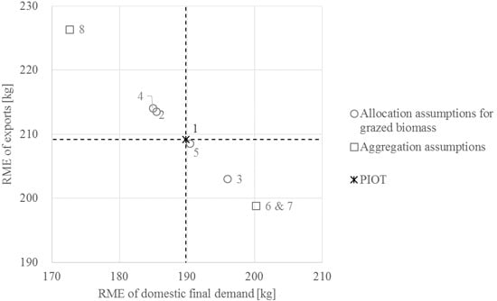
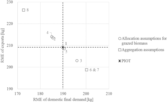
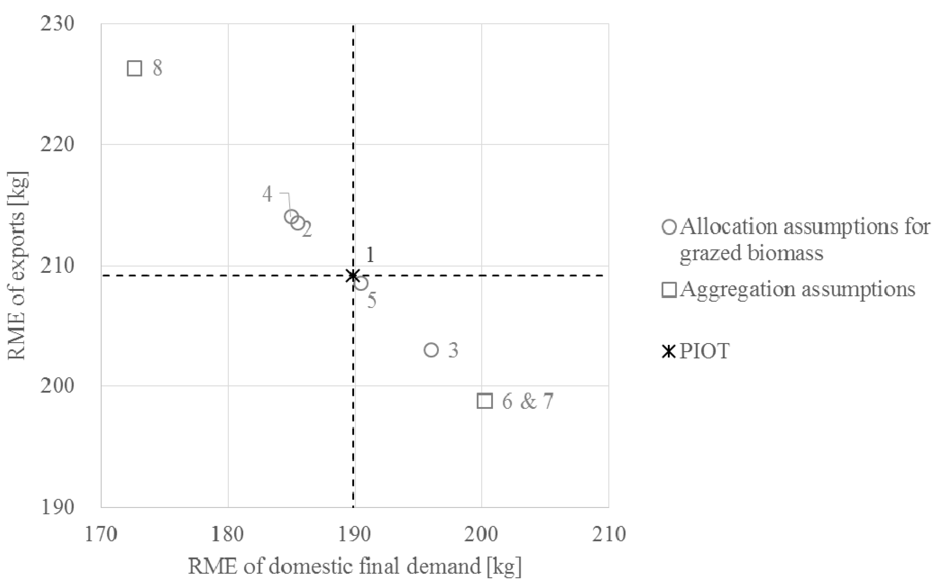
Due to the assumptions made in calculating RMC in an EEIOA-based approach given existing data constraints, the resulting indicator cannot be interpreted in the same manner as other material flow indicators that are calculated based purely on physical data. In this article, a simple hypothetical input-output model with material extensions is used to illustrate the impact of some of the most common assumptions in EEIOA on RMC results. Section 2 contains the description of the model and its extension and Section 3 presents results for different sets of assumptions in the calculation. The aim is to render the method and the data on which the RMC indicator is based comprehensible and its results interpretable for sustainability researchers and practitioners. The (political) interpretability of the RMC indicator is discussed in depth in Section 4, leading to the conclusion that RMC must be understood not as an extension or a replacement of DMC but as an entirely new indicator with its own potential messages for sustainability.

2. Exemplifying Possible Differences in Accounting for Raw Material Equivalents

MIOTs are the structural centerpiece of EEIOA. They are organized either by commodity groups or by economic activities and distinguish intermediate inputs and outputs within production from the output to final demand. Final demand can be reported at different levels of detail but usually includes government spending, investments, household spending, and exports. Input-output tables are like the cooking recipes of economies, detailing how much input from each economic activity (or of each commodity group) is required by other economic activities (or the production of commodity groups) in order to produce the specific mix of output required to meet final demand. MIOTs are routinely compiled by the national statistical institutes of most countries as part of the system of national accounts.

In order to calculate RMC-type indicators, the input-output table is extended with one or more vectors containing information on the resource requirements (e.g., material, energy, or land use, or emissions) of the production process. The environmental accounts from which the data for the extension stem are commonly not compiled in the same sectoral structure as the input-output tables. Material flows, which are the focus of the work presented here, are distinguished by material category instead. It is therefore necessary to construct an environmental extension for the EEIOA model based on the available data. In this construction, decisions as to the allocation of material flows to economic sectors have to be made. In the calculation of the RMC indicators, multipliers are derived through input-output analysis and express the direct and indirect material requirements associated with the production of one unit of monetary output to final demand. The size of these multipliers depends both on the size of the material flows included in the environmental extension and on the size and relative composition of the monetary input and output flows. The latter element is crucial for the interpretation of the RMC indicator because it bases calculations on monetary rather than on physical input-output tables as Leontief [5] originally proposed, which could be transformed into a table in monetary units using a vector of prices. The environmentally extended input-output analysis approach commonly used today in accounting for footprint-type indicators was developed by Leontief to assess the amount of pollution associated with the final demand for two commodities (wheat and cloth) in a highly simplified hypothetical economy. These calculations were based on an input-output table in physical units (yards of cloth and bushels of wheat). In RMC calculations, input-output tables in monetary units are used because the according data in physical units are hardly available [61].) PIOTs would provide material input data by sectors for EEIOA applications but do not commonly exist [61]. In the following, the assumptions that have to be made as a result of the lack of material flow data reported by sectors are exemplified using both a PIOT- and a MIOT-based approach to calculating RME for a hypothetical economy. The PIOT (which would not commonly exist for real-life applications) is chosen as a point of departure in order to illustrate first what results a physical accounting approach would yield and how the material extension would be pre-allocated to economic sectors in such a case. The MIOT (which would be available and also commonly used for real-life applications) will necessarily yield different EEIOA results because, if no PIOT is available, it has no structural link to the data in its material extension and because the system boundaries adhered to in monetary accounting are different from those physical accounting follows.

In order to make the differences between a physical and a monetary accounting approach visible, RME are calculated for a simplified hypothetical economy (Table 1). This economy consists of seven different economic activities: grassland-based, crop, forest-based, dairy, meat, wood, and cork production. The first three are primary activities and extract materials; the other four further process the materials extracted.

Table 1. Physical input-output table (PIOT) of the hypothetical economy. Flows are depicted in kilograms (kg); domestic extraction (DE) is reported in the bottom row.

	Intermediate Inputs							Final Demand		Total Output x
PIOT [kg]	Grassland production	Crop production	Forest production	Dairy production	Meat production	Wood production	Cork production	Domestic (yd)	Export (yex)
grassland production	1	2	0	50	60	0	0	0	0	113
crop production	0	10	0	40	70	0	0	20	30	170
forest production	0	1	10	0	0	60	45	0	0	116
dairy production	0	1	1	10	2	1	2	40	30	87
meat production	0	1	1	1	17	1	1	30	35	87
wood production	0	21	5	93	140	10	5	40	30	344
cork production	0	0	0	0	0	0	8	12	19	39
DE	113	170	116	-	-	-	-	-	-	399

Table 1. Physical input-output table (PIOT) of the hypothetical economy. Flows are depicted in kilograms (kg); domestic extraction (DE) is reported in the bottom row.

	Intermediate Inputs							Final Demand		Total Output x
PIOT [kg]	Grassland production	Crop production	Forest production	Dairy production	Meat production	Wood production	Cork production	Domestic (yd)	Export (yex)
grassland production	1	2	0	50	60	0	0	0	0	113
crop production	0	10	0	40	70	0	0	20	30	170
forest production	0	1	10	0	0	60	45	0	0	116
dairy production	0	1	1	10	2	1	2	40	30	87
meat production	0	1	1	1	17	1	1	30	35	87
wood production	0	21	5	93	140	10	5	40	30	344
cork production	0	0	0	0	0	0	8	12	19	39
DE	113	170	116	-	-	-	-	-	-	399

Next to the inter-industry input-output relations (intermediate inputs), the domestic and foreign final demand y and the total output x are included in the PIOT. The dairy production activity, for example, requires inputs from grassland and crop production to feed the animals and, at a lower level, uses some of its own production. It also receives substantial input from wood production used in building and maintaining stables and fences. The small input from meat production represents food provided to workers in dairy production. The output produced is mainly for final demand, out of which 40 kg are domestic and 30 kg are foreign (i.e., exports). The environmental extension to this input-output model is a row vector of domestic extraction (DE) by sector. DE is one of the central indicators of material flow accounting (MFA) and encompasses all materials extracted by and subject to further use in an economy (i.e., all biomass from agriculture, forestry or hunting, all fossil energy carriers, ores, and non-metallic minerals from mining). Data are collected in high detail and commonly reported by 45 different material types extracted domestically [75]. Non-market flows such as biomass grazed by animals, used crop residues, and the surrounding rock in mined metal ores are also accounted for because the inclusion of materials as DE is not dependent on their market value. According to MFA conventions, animals, along with humans and artifacts, are considered part of the socioeconomic (rather than the natural) system so that their feed intake from the natural system through grazing constitutes a form of domestic extraction [4,75,76]. The inclusion of non-market flows in physical accounting is the result of the system boundary definition, which differs substantially from the system boundary definition in monetary accounting. While in the former, flows are accounted for if they cross the boundary between the natural and the socioeconomic system, the system boundary in the latter accounting system is located where flows obtain monetary value. This difference in the system boundaries means that the physical and the monetary accounting approach may refer to comparable but not to identical systems. One possible response to this difference in system boundaries could lie in using a material extension to the MIOT, which corresponds to the system boundaries of the monetary accounting system. The resulting indicator would cover only a sub-set of the material flows commonly covered by material flow accounting. Existing EEIOA-based RMC or material footprint studies, however, contain all material extraction, including non-market flows, in their environmental extension. This, of course, is highly important in the interpretation of the calculated indicators.

By using a vector of prices (one price for the output of each economic activity), the PIOT can be transformed into a MIOT (Table 2). Although the MIOT is (partially) derived from the PIOT in this example, the two tables will be treated separately henceforth. The reason for no longer considering them as linked is two-fold: (1) For real-life EEIOA applications, no PIOT would be available and the allocation of material flows in the environmental extension cannot rely on information only available in a PIOT. (2) Due to the difference in system boundaries for physical and monetary accounting, the MIOT can only be understood in part as a direct translation of the PIOT into monetary terms. Market value is a precondition for inclusion in monetary accounts but not for inclusion in material flow accounts. A decision must therefore be made with regard to the allocation of non-market flows in the material extension to one of the market sectors in the input-output table. Next to grazed biomass, illustrated here, the most prominent non-market flows globally are used crop residues and waste rock extracted during mining activities. In 2010, these material flows accounted for 21% of global domestic extraction [77]. In countries where mining and/or animal husbandry play an important role, non-market flows make up more than half of material extraction [28,77,78].

Table 2. Monetary input-output table (MIOT) of the hypothetical economy. Flows are depicted in dollars ($); domestic extraction (DE) is reported in kilograms (kg) in the bottom row.

	Intermediate Inputs						Final Demand		Total Output x
MIOT [$]	crop production	forest production	dairy production	meat production	wood production	cork production	domestic (yd)	export (yex)
crop production	3	-	12	21	-	-	6	9	51
forest production	0	4	-	-	22	16	-	-	42
dairy production	1	1	10	2	1	2	40	30	87
meat production	10	10	10	170	10	10	300	350	870
wood production	2	1	9	14	1	1	4	3	34
cork production	-	-	-	-	-	24	36	57	117
DE [kg]	283	116	-	-	-	-	-	-	399

Table 2. Monetary input-output table (MIOT) of the hypothetical economy. Flows are depicted in dollars ($); domestic extraction (DE) is reported in kilograms (kg) in the bottom row.

	Intermediate Inputs						Final Demand		Total Output x
MIOT [$]	crop production	forest production	dairy production	meat production	wood production	cork production	domestic (yd)	export (yex)
crop production	3	-	12	21	-	-	6	9	51
forest production	0	4	-	-	22	16	-	-	42
dairy production	1	1	10	2	1	2	40	30	87
meat production	10	10	10	170	10	10	300	350	870
wood production	2	1	9	14	1	1	4	3	34
cork production	-	-	-	-	-	24	36	57	117
DE [kg]	283	116	-	-	-	-	-	-	399

In the hypothetical economy, biomass grazed by animals is the output of the grassland production sector in the PIOT but has no direct market value and therefore does appear in the MIOT. For the other activities, the following prices were assumed in calculating the MIOT: $0.30/kg for cropland, $0.36/kg for forest, $1.00/kg for dairy, $10.00/kg for meat, $0.10/kg for wood, and $3.00/kg for cork production.

In the MIOT, grazed biomass is included in the environmental extension and an assumption must be made in its allocation to one of the economic sectors. In Table 2, it was allocated to crop production. The different possibilities that exist for the allocation of this non-market flow in the environmental extension are presented and calculated in Section 3.

The technological A matrices, which include the coefficients of direct input requirements, can be calculated based on the PIOT and the MIOT by multiplying these matrices with the diagonalized inversion of the vector of total output x. A detailed description and discussion of the calculations required for this type of input-output analysis can be found in the textbook by Miller and Blair [6]. If Z is the matrix of intermediate inputs (see Table 1 and Table 2), then

$$A=Z{\widehat{x}}^{-1}$$

(1)

where ${\widehat{x}}^{-1}$ is the diagonalized inversion of x. Each entry in the resulting A matrix reports direct input requirements per unit of total output in either kg/kg if the calculation is based on the PIOT (Table 3a) or in $/$ if the calculation is based on the MIOT (Table 3b). In the latter case, the environmental extension is in kg/$.

While the A matrices in Table 3 provide information on direct material requirements, the Leontief inverse includes the multipliers for direct and indirect requirements. The Leontief inverse L is expressed as L = (I − A)⁻¹ where I is the identity matrix with ones along the diagonal and zeroes everywhere else and A is the technological matrix of direct requirements. The Leontief inverse is derived from

$$x={\left(I-A\right)}^{-1}\times y$$

(2)

where x is total output and y is final demand (for a detailed description, see [6]).

This calculation can be performed based either on the physical (Table 3a) or the monetary (Table 3b) A matrix. The direct and indirect material requirements associated with a given level of final demand are calculated based on the Leontief inverse (Table 4) with its material extension. Final demand (domestic and foreign) is reported in physical units in the PIOT and in monetary units in the MIOT; the RME of both types of final demand can be calculated by multiplying final demand with the multipliers in the material extension of the Leontief inverse.

Table 3. Technological A matrices based on the physical input-output table (A_P in Table 3a, top) in kilograms per kilogram (kg/kg) and based on the monetary input-output table (A_M in Table 3b, bottom) in dollars per dollar ($/$) and kilograms per dollar (kg/$) for the material extension of domestic extraction (DE).

AP [kg/kg]	Grassland production	Crop production	Forest production	Dairy production	Meat production	Wood production	Cork production
grassland production	0.0	0.0	-	0.6	0.7	-	-
crop production	-	0.1	-	0.5	0.8	-	-
forest production	-	0.0	0.1	-	-	0.2	1.2
dairy production	-	0.0	0.0	0.1	0.0	0.0	0.1
meat production	-	0.0	0.0	0.0	0.2	0.0	0.0
wood production	-	0.1	0.0	1.1	1.6	0.0	0.1
cork production	-	-	-	-	-	-	0.2
DE	1.00	1.00	1.00	-	-	-	-

AP [kg/kg]	Grassland production	Crop production	Forest production	Dairy production	Meat production	Wood production	Cork production
grassland production	0.0	0.0	-	0.6	0.7	-	-
crop production	-	0.1	-	0.5	0.8	-	-
forest production	-	0.0	0.1	-	-	0.2	1.2
dairy production	-	0.0	0.0	0.1	0.0	0.0	0.1
meat production	-	0.0	0.0	0.0	0.2	0.0	0.0
wood production	-	0.1	0.0	1.1	1.6	0.0	0.1
cork production	-	-	-	-	-	-	0.2
DE	1.00	1.00	1.00	-	-	-	-

AM [$/$]	Crop production	Forest production	Dairy production	Meat production	Wood production	Cork production
crop production	0.1	-	0.1	0.0	-	-
forest production	0.0	0.1	-	-	0.6	0.1
dairy production	0.0	0.0	0.1	0.0	0.0	0.0
meat production	0.2	0.2	0.1	0.2	0.3	0.1
wood production	0.0	0.0	0.1	0.0	0.0	0.0
cork production	-	-	-	-	-	0.2
DE [kg/$]	5.55	2.78	-	-	-	-

AM [$/$]	Crop production	Forest production	Dairy production	Meat production	Wood production	Cork production
crop production	0.1	-	0.1	0.0	-	-
forest production	0.0	0.1	-	-	0.6	0.1
dairy production	0.0	0.0	0.1	0.0	0.0	0.0
meat production	0.2	0.2	0.1	0.2	0.3	0.1
wood production	0.0	0.0	0.1	0.0	0.0	0.0
cork production	-	-	-	-	-	0.2
DE [kg/$]	5.55	2.78	-	-	-	-

Table 4. Leontief inverses based on the physical input-output table (L_P in Table 4a, top) in kilograms per kilogram (kg/kg) and based on the monetary input-output table (L_M in Table 4b, bottom) in dollars per dollar ($/$) and kilograms per dollar (kg/$) for the material extension of domestic extraction (DE).

LP [kg/kg]	Grassland production	Crop production	Forest production	Dairy production	Meat production	Wood production	Cork production
grassland production	1.0	0.0	0.0	0.7	0.9	0.0	0.1
crop production	-	1.1	0.0	0.6	1.1	0.0	0.1
forest production	0.0	0.0	1.1	0.3	0.4	0.2	1.7
dairy production	-	0.0	0.0	1.1	0.1	0.0	0.1
meat production	0.0	0.0	0.0	0.0	1.3	0.0	0.1
wood production	-	0.2	0.1	1.4	2.3	1.1	0.5
cork production	-	-	-	-	-	-	1.3
DE	1.01	1.14	1.14	1.54	2.48	0.22	1.87

LP [kg/kg]	Grassland production	Crop production	Forest production	Dairy production	Meat production	Wood production	Cork production
grassland production	1.0	0.0	0.0	0.7	0.9	0.0	0.1
crop production	-	1.1	0.0	0.6	1.1	0.0	0.1
forest production	0.0	0.0	1.1	0.3	0.4	0.2	1.7
dairy production	-	0.0	0.0	1.1	0.1	0.0	0.1
meat production	0.0	0.0	0.0	0.0	1.3	0.0	0.1
wood production	-	0.2	0.1	1.4	2.3	1.1	0.5
cork production	-	-	-	-	-	-	1.3
DE	1.01	1.14	1.14	1.54	2.48	0.22	1.87

LM [$/$]	Crop production	Forest production	Dairy production	Meat production	Wood production	Cork production
crop production	1.1	0.0	0.2	0.0	0.0	0.0
forest production	0.0	1.1	0.1	0.0	0.7	0.2
dairy production	0.0	0.0	1.1	0.0	0.1	0.0
meat production	0.3	0.3	0.3	1.3	0.6	0.2
wood production	0.1	0.0	0.1	0.0	1.1	0.0
cork production	-	-	-	-	-	1.3
DE [kg/$]	6.09	3.17	1.24	0.23	2.15	0.61

LM [$/$]	Crop production	Forest production	Dairy production	Meat production	Wood production	Cork production
crop production	1.1	0.0	0.2	0.0	0.0	0.0
forest production	0.0	1.1	0.1	0.0	0.7	0.2
dairy production	0.0	0.0	1.1	0.0	0.1	0.0
meat production	0.3	0.3	0.3	1.3	0.6	0.2
wood production	0.1	0.0	0.1	0.0	1.1	0.0
cork production	-	-	-	-	-	1.3
DE [kg/$]	6.09	3.17	1.24	0.23	2.15	0.61

3. Results Vary Depending on Commonly Made Assumptions

If both the PIOT and the MIOT were available for real-life application, as is the case in the example of the hypothetical economy, no assumptions in the allocation of material flows to the extension of the MIOT would have to be made. The necessary information on the use of physical flows by sector is included in the PIOT. However, because physical input-output data are generally not available for real-life applications, allocation decisions have to be made by researchers constructing the material extension to a MIOT for EEIOA approaches. In order to illustrate the impact of the assumptions on the results, the following calculations are based on the MIOT and not on the original PIOT. Using the environmentally extended input-output model of a hypothetical economy, which was introduced in Section 2, RME results are calculated for different sectoral material allocations.

As was shown in the literature review in Section 1.2, sectoral aggregation has been identified as playing a crucial role in the results of EEIOA calculations. The more highly aggregated the sectors are, the more likely it is that different products and products sold at different prices to intermediate uses and final demand are grouped together, violating the assumptions of price and product homogeneity. RME indicators have been calculated for different levels of sectoral aggregation to illustrate the impact this may have on the results. The RME of domestic final demand are calculated separately from the RME of exports to illustrate how the assumptions result in changing allocations of material requirements to domestic and foreign final demand. The MIOT, if it cannot be derived from an existing PIOT via a vector of homogenous prices [5,61], cannot replicate the results of the PIOT. Since the physical and the monetary accounting system refer to different system boundaries, the difference in results they yield must not be understood as an expression of one being correct and one being erroneous. Instead, the difference makes abundantly clear that the indicators derived from physical accounting must be interpreted in a manner altogether different from the one that is appropriate for indicators derived from mixed physical and monetary accounting in EEIOA.

In the initial calculations for a hypothetical economy (Section 2), one assumption was already made in the allocation of grazed biomass to one of economic activities (cropland production) depicted in the MIOT in the construction of the material extension (see Table 2). Of course, the MIOT in which such an allocation in the material extension has occurred can no longer replicate the results of the PIOT, which features grassland production as one of its sectors. In the PIOT-based calculations, the RME of domestic final demand amount to 190 kg while the RME of exports are 209 kg. Based on the MIOT with its particular environmental extension, the RME of domestic final demand are lower (185 kg) and the RME of exports are higher (214 kg). Because this and all other assumptions tested in this article consist of equivalence operations, the sum of the material extension (in this case 399 kg of domestic extraction, see Table 1 and Table 2) does not change but its allocation to domestic and foreign final demand does. The allocation of grazed biomass illustrates that where the MIOT cannot be based on the PIOT, an allocation decision must be made in the material extension, which will have an impact on the results. In existing studies on the RMC, no PIOTs were available [61] so that all material in the extension was initially allocated to sectors based on researchers’ assumptions.

Through its inclusion of non-market flows, the PIOT has a higher degree of sectoral detail than the MIOT. Due to the difference in system boundary definitions and the data limitation in the MIOT, grazed biomass is distributed differently than it would be in the PIOT, leading to a difference in the results obtained. In material extensions for input-output tables, non-market material flows are commonly allocated to an existing economic activity, following use logic: For example, grazed biomass could be allocated to the activity that requires it as an input, such as cattle, meat, or milk production [79]. The allocation of grazed biomass as a non-market flow causes a change in the results ranging between +3.2% for the RME of domestic final demand and −2.9% for the RME of exports when grazed biomass is allocated to dairy production (calculation 3 in Table 5) and −2.6% for domestic final demand and +2.4% for exports when grazed biomass is allocated to meat production (calculation 4 in Table 5). Distributing the grazed biomass to both the dairy and the meat production activity in physically equal shares (calculation 5 in Table 5) causes the lowest change compared to the results of the PIOT-based calculation. Of course, if the PIOT were available for real-life applications, none of these assumptions would have to be made. Instead, an input-output table in mixed units (e.g., physical units for material flows and monetary units to more accurately cover services) could be used. In practice, however, where no PIOT is available, the type of assumptions listed in Table 5 are commonly made.

Table 5. Impact of sectoral allocation assumptions for grazed biomass on the raw material equivalents in kilograms (kg) based on the physical input-output table (PIOT) and the monetary input-output table (MIOT).

	Basis	Assumptions	Raw material equivalents of
			Domestic final demand [kg]	Exports [kg]
1	PIOT	/	189.9	209.1
2	MIOT	grazed biomass allocated to crop production	185.5	213.5
3	MIOT	grazed biomass allocated to dairy production	195.9	203.1
4	MIOT	grazed biomass allocated to meat production	184.9	214.1
5	MIOT	grazed biomass allocated to dairy (50%) and meat (50%) production	190.4	208.6

Table 5. Impact of sectoral allocation assumptions for grazed biomass on the raw material equivalents in kilograms (kg) based on the physical input-output table (PIOT) and the monetary input-output table (MIOT).

	Basis	Assumptions	Raw material equivalents of
			Domestic final demand [kg]	Exports [kg]
1	PIOT	/	189.9	209.1
2	MIOT	grazed biomass allocated to crop production	185.5	213.5
3	MIOT	grazed biomass allocated to dairy production	195.9	203.1
4	MIOT	grazed biomass allocated to meat production	184.9	214.1
5	MIOT	grazed biomass allocated to dairy (50%) and meat (50%) production	190.4	208.6

The assumption of product homogeneity is more likely to be violated the more highly aggregated a given input-output table is. The World Input-Output Database (WIOD) and a number of national input-output tables, such as Austria’s, for example, report all mining and quarrying as one activity [80,81] and thus group very different products together. Especially for smaller economies with a limited domestic resource base, this aggregated level of reporting may be necessary to protect the confidential data of individual business operations. In such cases, the average price ($/kg) of the output of the mining and quarrying activity is unlikely to be equally fitting for construction sand, petroleum, and gold ore. If metal and fossil fuel mining are grouped into the same category, domestic extraction of waste rock associated with the mining of ore would also find its way into the fossil energy carrier supply chain. In order to make the impact of the level of aggregation (and the associated product and price inhomogeneity) on the results visible, the input-output tables (Table 1 and Table 2) are aggregated from seven to three activities: agriculture and forestry (grassland, crop, and forest production), food production (dairy and meat production), and wood and cork production.

The results in Table 6 show that the impact of the level of sectoral aggregation on the RME results is stronger than the impact of the sectoral allocation of grazed biomass in the construction of the environmental extension. Of course, if a detailed table is available, it should not be additionally aggregated. These examples serve to illustrate how a calculation based on a more highly aggregated table would yield different results than the same calculation based on a more disaggregated table if it were available. This example has very real implications if results are compared for different countries that have input-output tables available at differing levels of aggregation or if such tables at different levels of aggregation are linked in an MRIO model [82].

Table 6. Impact of aggregation on the raw material equivalents in kilograms (kg) based on the physical input-output table (PIOT) and the monetary input-output table (MIOT).

	Basis	Assumptions	Raw material equivalents of
			Domestic final demand [kg]	Exports [kg]
6	PIOT	aggregation to 3 economic activities	200.2	198.8
7	MIOT	aggregation to 3 economic activities (calculated from aggregated PIOT)	200.2	198.8
8	MIOT	aggregation to 3 economic activities (aggregated from 7 activity MIOT)	172.6	226.4

Table 6. Impact of aggregation on the raw material equivalents in kilograms (kg) based on the physical input-output table (PIOT) and the monetary input-output table (MIOT).

	Basis	Assumptions	Raw material equivalents of
			Domestic final demand [kg]	Exports [kg]
6	PIOT	aggregation to 3 economic activities	200.2	198.8
7	MIOT	aggregation to 3 economic activities (calculated from aggregated PIOT)	200.2	198.8
8	MIOT	aggregation to 3 economic activities (aggregated from 7 activity MIOT)	172.6	226.4

When it is aggregated to three economic activities, the PIOT allocates approximately 200 kg of RME to domestic final demand (+5.4% compared to the more disaggregated table) and 199 kg to exports (−4.9% compared to the more disaggregated table). If the aggregated MIOT is constructed using weighted average prices based on the aggregated total output of the seven-activity PIOT and MIOT (calculation 7 in Table 6), the results are identical to those based on the aggregated PIOT (calculation 6 in Table 6). At this level of aggregation, the difference in results that occurred previously due to the allocation of grazed biomass (see Table 5) is no longer relevant because grazed biomass is allocated to the agriculture and forestry activity in both tables. If, however, the disaggregated MIOT (Table 2) is aggregated to the three activities (calculation 8 in Table 6), the results change quite drastically. The RME of domestic final demand decrease by 9.1% compared to the calculation based on the disaggregated PIOT and the RME of exports increase by 8.1%. Important information about the composition of each of the economic activities is lost when the aggregation cannot be based on the relative size of physical flows.

Each assumption on which calculations 2–8 for the RME of final demand were based resulted in a change in the results, not just compared to the PIOT-based calculation, as was to be expected, but also as compared to the other MIOT-based calculations (Figure 1). Three sets of assumptions commonly made in the MIOT-based calculation result in a higher RME of exports and lower RME of domestic final demand compared to the PIOT-based calculation:

-

grazed biomass as a non-market flow is allocated to crop production as an economic activity (calculation 2),

-

grazed biomass is allocated to meat production (calculation 4), and

-

aggregation of the seven-activity MIOT to three activities (calculation 8).

A larger RME of domestic final demand and a lower RME of exports than in the PIOT-based calculation is caused by four assumptions:

-

grazed biomass as a non-market flow is allocated in equal shares to dairy production and meat production as economic activities (calculation 5),

-

grazed biomass is allocated to dairy production (calculation 3),

-

aggregation of the PIOT to three economic activities (calculation 6), and

-

construction of a MIOT aggregated to three economic activities based on the aggregated PIOT (calculation 7).

Figure 1. Variation of raw material equivalents (RME) in kilograms (kg) with changing assumptions. At the center of the crosshairs is the result of the physical input-output table (PIOT, point 1). To the top and left of point 1 are results in which the RME of domestic final demand are lower and of exports are higher; to the bottom and right of point 1 are results in which the RME of domestic final demand are higher and of exports are lower. Points: 2 grazed biomass allocated to crop production, 3 grazed biomass allocated to dairy production, 4 grazed biomass allocated to meat production, 5 grazed biomass allocated to dairy (50%) and meat (50%) production, 6 aggregation to three economic activities, 7 aggregation to three economic activities (calculated from aggregated PIOT), and 8 aggregation to three economic activities (aggregated from seven activity MIOT).

Figure 1. Variation of raw material equivalents (RME) in kilograms (kg) with changing assumptions. At the center of the crosshairs is the result of the physical input-output table (PIOT, point 1). To the top and left of point 1 are results in which the RME of domestic final demand are lower and of exports are higher; to the bottom and right of point 1 are results in which the RME of domestic final demand are higher and of exports are lower. Points: 2 grazed biomass allocated to crop production, 3 grazed biomass allocated to dairy production, 4 grazed biomass allocated to meat production, 5 grazed biomass allocated to dairy (50%) and meat (50%) production, 6 aggregation to three economic activities, 7 aggregation to three economic activities (calculated from aggregated PIOT), and 8 aggregation to three economic activities (aggregated from seven activity MIOT).

Since all assumptions reflected in calculations 2–8 involve equivalence operations, the sum of the material extension data (399 kg of domestic extraction) does not change although its allocation to the two types of final demand does. In Figure 1, these results can therefore all be plotted along a diagonal with f(x) = 399 − x.

4. Implications for Indicator Interpretation

The RME results obtained in the PIOT-based calculation differ from the results of the MIOT-based calculation. In the example presented in Section 3, errors violating the correspondence between the MIOT- and the PIOT-based results were knowingly introduced and could have been avoided or corrected. In real-life EEIOA applications, however, for which PIOTs are not available, such corrections cannot be made. Due to the limited proportionality between the monetary and the physical flows in an economy, the MIOT cannot be interpreted as equivalent to a PIOT, especially for quantitatively large material flows such as construction minerals or grazed biomass. The Leontief inverse based on MIOTs does not distribute material flows in a comparable manner to a PIOT if the assumption of homogenous products and prices is violated, as is generally the case [43].

The main consequence of what has been shown in Section 3 is that MIOT-based RMC indicators may not be interpreted as though they were PIOT-based. Instead, the logic that the MIOT implies is conceptually most strongly related to the allocation of environmental burden by economic value in life cycle assessment [52]). While this is obvious to researchers calculating MIOT-based RMC, it is often not quite as clear to sustainability researchers not working with EEIOA approaches and much less so to practitioners and policy makers. The differences between PIOT- and MIOT-based RMC are crucial in explaining why the available RMC indicators might not react to sustainability policies and instruments in the expected manner. For example, higher spending within one category of final demand increases the associated RME. If a high-price version of a product is offered for domestic final demand and the same product is exported in a low-price version, the RME of domestic final demand will appear to be higher even though the required material inputs may not increase proportionally to the price. The indicator may therefore not be able to fully reflect the (potentially resource-saving) impact of the consumption of higher-cost products made with lower inputs [83]. This would be the case if more expensive carbon-labeled products (with lower fossil energy inputs) were produced for domestic final consumption and non-carbon-labeled, less expensive versions of the same product were produced for export.

The calculation of RMC also has important implications for the assessment of resource efficiency based on this indicator. Resource efficiency is a measure of the amount of wealth generated with one unit of material use and is commonly calculated as GDP per DMC. In order to take outsourcing of resource-intensive industries into account in assessing a country’s resource efficiency, it is currently deemed more suitable to express resource efficiency as GDP per RMC [25]. GDP, however, is calculated (in the expenditure approach) as the sum of the final demand categories household consumption, government expenditure, capital formation, and net exports [66]. The EEIOA-based RMC indicator is calculated based on domestic final demand consisting of household consumption, capital formation, and government expenditure while monetary exports (including re-exports) represent foreign final demand and imports are included in the RMC if they are directly consumed or indirectly required to satisfy domestic final demand. Because both GDP and RMC include the same measure of domestic final demand (household consumption, capital formation, and government expenditure), these two indicators cannot be treated as independent ex ante, possibly limiting possibilities for statistical analyses of resource efficiency calculated as GDP per RMC.

Finally, RMC is often interpreted such that economies should be held accountable for the environmental impacts associated with their final consumption, no matter where they occur [29]. However, exports not only entail environmental burden but also socioeconomic benefits (in terms of revenue, labor market, and infrastructure developments) associated with their production (see Section 1.1). Wiedmann and colleagues [9] show that the material footprint (term used instead of RMC) of exports was especially high for China in 2008; that same year, exports contributed almost 35% to Chinese GDP [84]. By comparison, in the United States of America, with its significantly lower material footprint of exports, this share was approximately 13%. It cannot be argued that by domestically supplying materials for consumption in other countries, China is striking a deal from which it does not also benefit. Rigorous scrutiny of the (political) message conveyed by the RMC indicator is necessary and must cover the identification of the appropriate addressee: In contrast to standard material flow indicators, the RMC does not reflect activity on a territory corresponding to a defined political mandate. Wiedmann and colleagues [9] indicate that almost one quarter of China’s domestic extraction winds up in other countries’ RMC. Politicians in the latter countries, however, have no mandate that would allow them to reduce resource use associated with production in China.

5. Conclusions

The RMC indicator, as currently calculated in MIOT-based approaches, provides a measure of the material flows to which reported monetary flows correspond based on several key assumptions: The RME of imports of country A are those material inputs, no matter where in the world they occur, that have been distributed (via allocation in the environmental extension) alongside monetary flows in the global production system that were required to produce the monetary imports for final demand of country A, assuming that each economic sector in country A and in all of its trade partners produces only one specific product that is sold at the same price throughout the production system and to different types of final demand [15].

The RMC thus provides a different perspective on the overall size of an economy compared to GDP as a purely monetary and to DMC as a purely physical indicator. GDP has little direct explanatory power for environmental pressures and is still under development in important regards such as accounting for informal economic activity. DMC seeks to represent domestic production structures and material use on a specific territory but is unable to capture the impacts of the increasing fragmentation of global supply and use chains. RMC was developed in an attempt to respond to this perceived short-coming of the DMC indicator.

In the scientific quest for a robust indicator of the size of an economy that can be interpreted in a meaningful way to gauge that economy’s sustainability, the RMC is a relatively new attempt to offer information that previously existing indicators (in this case, the DMC) could not cover. The RMC, as an indicator reflecting both monetary and physical developments, cannot, however, replace the DMC. Next to the scope of information offered by each of these indicators, a very promising future research endeavor will lie in analyzing DMC and RMC in relation to one another: How do countries’ patterns of trade and consumption change when not only material flows but also monetary flows are taken into account? What does this relationship tell us with regard to drivers of material use? Are the same drivers at play in different countries? In answering these and related questions, important advances in not only monitoring but understanding what drives material use can be made. The latter is a precondition to conceptualizing and possibly implementing a much-needed transition towards greater sustainability.

References

1. Waas, T.; Hugé, J.; Block, T.; Wright, T.; Benitez-Capistros, F.; Verbruggen, A. Sustainability Assessment and Indicators: Tools in a Decision-Making Strategy for Sustainable Development. Sustainability 2014, 6, 5512–5534. [Google Scholar] [CrossRef] [Green Version]
2. Baldwin, R.E. Global Supply Chains: Why They Emerged, Why They Matter, and Where They Are Going; Centre for Economic Policy Research: London, UK, 2012. [Google Scholar]
3. WTO. World Trade Report 2008: Trade in a Globalizing World; World Trade Organization (WTO): Geneva, Switzerland, 2008. [Google Scholar]
4. Fischer-Kowalski, M.; Krausmann, F.; Giljum, S.; Lutter, S.; Mayer, A.; Bringezu, S.; Moriguchi, Y.; Schütz, H.; Schandl, H.; Weisz, H. Methodology and Indicators of Economy—Wide Material Flow Accounting. J. Ind. Ecol. 2011, 15, 855–876. [Google Scholar] [CrossRef]
5. Leontief, W. Environmental repercussions and the economic structure: An input-output approach. Rev. Econ. Stat. 1970, 52, 262–271. [Google Scholar] [CrossRef]
6. Miller, R.E.; Blair, P.D. Input-Output Analysis: Foundations and Extensions; Cambridge University Press: Cambridge, UK, 2009. [Google Scholar]
7. Schoer, K.; Weinzettel, J.; Kovanda, J.; Giegrich, J.; Lauwigi, C. Raw Material Consumption of the European Union—Concept, Calculation Method, and Results. Environ. Sci. Technol. 2012, 46, 8903–8909. [Google Scholar] [CrossRef] [PubMed]
8. Tukker, A.; de Koning, A.; Wood, R.; Hawkins, T.; Lutter, S.; Acosta, J.; Rueda Cantuche, J.M.; Bouwmeester, M.; Oosterhaven, J.; Drosdowski, T.; et al. Exiopol—Development and Illustrative Analyses of a Detailed Global MR EE SUT/IOT. Econ. Syst. Res. 2013, 25, 50–70. [Google Scholar] [CrossRef]
9. Wiedmann, T.O.; Schandl, H.; Lenzen, M.; Moran, D.; Suh, S.; West, J.; Kanemoto, K. The material footprint of nations. Proc. Natl. Acad. Sci. USA 2013. [Google Scholar] [CrossRef]
10. Fang, K.; Heijungs, R.; de Snoo, G.R. Theoretical exploration for the combination of the ecological, energy, carbon, and water footprints: Overview of a footprint family. Ecol. Indic. 2014, 36, 508–518. [Google Scholar] [CrossRef]
11. Liu, Z.; Geng, Y.; Lindner, S.; Zhao, H.; Fujita, T.; Guan, D. Embodied energy use in China’s industrial sectors. Energy Policy 2012, 49, 751–758. [Google Scholar] [CrossRef]
12. Peters, G.P. From production-based to consumption-based national emission inventories. Ecol. Econ. 2008, 65, 13–23. [Google Scholar] [CrossRef]
13. Peters, G.P.; Minx, J.C.; Weber, C.L.; Edenhofer, O. Growth in emission transfers via international trade from 1990 to 2008. Proc. Natl. Acad. Sci. 2011, 108, 8903–8908. [Google Scholar] [CrossRef] [PubMed]
14. Munksgaard, J.; Pedersen, K.A. CO2 accounts for open economies: Producer or consumer responsibility? Energy Policy 2001, 29, 327–334. [Google Scholar] [CrossRef]
15. Schaffartzik, A.; Haberl, H.; Kastner, T.; Wiedenhofer, D.; Eisenmenger, N.; Erb, K.-H. Trading Land: A Review of Approaches to Accounting for Upstream Land Requirements of Traded Products. J. Ind. Ecol. 2015. [Google Scholar] [CrossRef]
16. Bruckner, M.; Fischer, G.; Tramberend, S.; Giljum, S. Measuring telecouplings in the global land system: A review and comparative evaluation of land footprint accounting methods. Ecol. Econ. 2015, 114, 11–21. [Google Scholar] [CrossRef]
17. Turner, K.; Lenzen, M.; Wiedmann, T.; Barrett, J. Examining the global environmental impact of regional consumption activities—Part 1: A technical note on combining input-output and ecological footprint analysis. Ecol. Econ. 2007, 62, 37–44. [Google Scholar] [CrossRef]
18. Wiedmann, T.; Minx, J.; Barrett, J.; Wackernagel, M. Allocating ecological footprints to final consumption categories with input-output analysis. Ecol. Econ. 2006, 56, 28–48. [Google Scholar] [CrossRef]
19. Daniels, P.L.; Lenzen, M.; Kenway, S.J. The Ins and Outs of Water Use—A Review of Multi-Region Input-Output Analysis and Water Footprints for Regional Sustainability Analysis and Policy. Econ. Syst. Res. 2011, 23, 353–370. [Google Scholar] [CrossRef]
20. Lenzen, M.; Moran, D.; Kanemoto, K.; Foran, B.; Lobefaro, L.; Geschke, A. International trade drives biodiversity threats in developing nations. Nature 2012, 486, 109–112. [Google Scholar] [CrossRef] [PubMed]
21. Simas, M.S.; Golsteijn, L.; Huijbregts, M.A.J.; Wood, R.; Hertwich, E.G. The “Bad Labor” Footprint: Quantifying the Social Impacts of Globalization. Sustainability 2014, 6, 7514–7540. [Google Scholar] [CrossRef] [Green Version]
22. Alsamawi, A.; Murray, J.; Lenzen, M. The Employment Footprints of Nations. J. Ind. Ecol. 2014, 18, 59–70. [Google Scholar] [CrossRef]
23. Alsamawi, A.; Murray, J.; Lenzen, M.; Moran, D.; Kanemoto, K. The Inequality Footprints of Nations: A Novel Approach to Quantitative Accounting of Income Inequality. PLoS ONE 2014, 9, e110881. [Google Scholar] [CrossRef] [PubMed] [Green Version]
24. European Commission. Communication from the Commission to the European Parliament, the Council, the European Economic and Social Committee and the Committee of the Regions: Roadmap to a Resource Efficient Europe; European Commission: Brussels, Belgium, 2011. [Google Scholar]
25. European Commission. Environment: Higher recycling targets to drive transition to a Circular Economy with new jobs and sustainable growth. In Press Releases Database; European Commission: Brussels, Belgium, 2014. [Google Scholar]
26. Weisz, H.; Krausmann, F.; Amann, C.; Eisenmenger, N.; Erb, K.-H.; Hubacek, K.; Fischer-Kowalski, M. The physical economy of the European Union: Cross-country comparison and determinants of material consumption. Ecol. Econ. 2006, 58, 676–698. [Google Scholar] [CrossRef]
27. Fischer-Kowalski, M.; Amann, C. Beyond IPAT and Kuznets Curves: Globalization as a Vital Factor in Analysing the Environmental Impact of Socio-Economic Metabolism. Popul. Environ. 2001, 23, 7–47. [Google Scholar] [CrossRef]
28. Giljum, S. Trade, Materials Flows, and Economic Development in the South: The Example of Chile. J. Ind. Ecol. 2004, 8, 241–261. [Google Scholar] [CrossRef]
29. Jakob, M.; Marschinski, R. Interpreting trade-related CO2 emission transfers. Nat. Clim. Chang. 2012, 3, 19–23. [Google Scholar] [CrossRef]
30. Muradian, R.; O’Connor, M.; Martinez-Alier, J. Embodied pollution in trade: Estimating the “environmental load displacement” of industrialised countries. Ecol. Econ. 2002, 41, 51–67. [Google Scholar] [CrossRef]
31. Ferng, J.-J. Allocating the responsibility of CO2 over-emissions from the perspectives of benefit principle and ecological deficit. Ecol. Econ. 2003, 46, 121–141. [Google Scholar] [CrossRef]
32. Bastianoni, S.; Pulselli, F.M.; Tiezzi, E. The problem of assigning responsibility for greenhouse gas emissions. Ecol. Econ. 2004, 49, 253–257. [Google Scholar] [CrossRef]
33. Gallego, B.; Lenzen, M. A consistent input-output formulation of shared producer and consumer responsibility. Econ. Syst. Res. 2005, 17, 365–391. [Google Scholar] [CrossRef]
34. Lenzen, M.; Murray, J.; Sack, F.; Wiedmann, T. Shared producer and consumer responsibility—Theory and practice. Ecol. Econ. 2007, 61, 27–42. [Google Scholar] [CrossRef]
35. Wood, R.; Hawkins, T.R.; Hertwich, E.G.; Tukker, A. Harmonising National Input-Output Tables for Consumption-Based Accounting—Experiences from Exiopol. Econ. Syst. Res. 2014, 26, 387–409. [Google Scholar] [CrossRef]
36. Geschke, A.; Wood, R.; Kanemoto, K.; Lenzen, M.; Moran, D. Investigating Alternative Approaches to Harmonise Multi-Regional Input-Output Data. Econ. Syst. Res. 2014, 26, 354–385. [Google Scholar] [CrossRef]
37. Wenz, L.; Willner, S.N.; Radebach, A.; Bierkandt, R.; Steckel, J.C.; Levermann, A. Regional and Sectoral Disaggregation of Multi-Regional Input-Output Tables—A Flexible Algorithm. Econ. Syst. Res. 2014. [Google Scholar] [CrossRef]
38. Kastner, T.; Schaffartzik, A.; Eisenmenger, N.; Erb, K.-H.; Haberl, H.; Krausmann, F. Cropland area embodied in international trade: Contradictory results from different approaches. Ecol. Econ. 2014, 104, 140–144. [Google Scholar] [CrossRef]
39. Liang, S.; Zhang, T. Investigating Reasons for Differences in the Results of Environmental, Physical, and Hybrid Input-Output Models. J. Ind. Ecol. 2013, 17, 432–439. [Google Scholar] [CrossRef]
40. Owen, A.; Steen-Olsen, K.; Barrett, J.; Wiedmann, T.; Lenzen, M. A Structural Decomposition Approach to Comparing Mrio Databases. Econ. Syst. Res. 2014, 26, 262–283. [Google Scholar] [CrossRef]
41. Moran, D.; Wood, R. Convergence between the Eora, Wiod, Exiobase, and Openeu’s Consumption-Based Carbon Accounts. Econ. Syst. Res. 2014, 26, 245–261. [Google Scholar] [CrossRef]
42. Lenzen, M.; Murray, S.A. A modified ecological footprint method and its application to Australia. Ecol. Econ. 2001, 37, 229–255. [Google Scholar] [CrossRef]
43. Hubacek, K.; Giljum, S. Applying physical input–output analysis to estimate land appropriation (ecological footprints) of international trade activities. Ecol. Econ. 2003, 44, 137–151. [Google Scholar] [CrossRef]
44. Hawkins, T.; Hendrickson, C.; Higgins, C.; Matthews, H.S.; Suh, S. A mixed-unit input-output model for environmental life-cycle assessment and material flow analysis. Environ. Sci. Technol. 2007, 41, 1024–1031. [Google Scholar] [CrossRef] [PubMed]
45. Giljum, S.; Hubacek, K.; Sun, L. Beyond the simple material balance: A reply to Sangwon Suh’s note on physical input-output analysis. Ecol. Econ. 2004, 48, 19–22. [Google Scholar] [CrossRef]
46. Suh, S. A note on the calculus for physical input-output analysis and its application to land appropriation of international trade activities. Ecol. Econ. 2004, 48, 9–17. [Google Scholar] [CrossRef]
47. Lenzen, M. Aggregation versus Disaggregation in Input-Output Analysis of the Environment. Econ. Syst. Res. 2011, 23, 73–89. [Google Scholar] [CrossRef]
48. Bouwmeester, M.C.; Oosterhaven, J. Specification and Aggregation Errors in Environmentally Extended Input-Output Models. Environ. Resour. Econ. 2013, 56, 307–335. [Google Scholar] [CrossRef]
49. Andrew, R.; Peters, G.P.; Lennox, J. Approximation and regional aggregation in multi-regional input-output analysis for national carbon footprint accounting. Econ. Syst. Res. 2009, 21, 311–335. [Google Scholar] [CrossRef]
50. Steen-Olsen, K.; Owen, A.; Hertwich, E.G.; Lenzen, M. Effects of Sector Aggregation on CO2 Multipliers in Multiregional Input-Output Analyses. Econ. Syst. Res. 2014, 26, 1–19. [Google Scholar] [CrossRef]
51. Su, B.; Huang, H.C.; Ang, B.W.; Zhou, P. Input-output analysis of CO2 emissions embodied in trade: The effects of sector aggregation. Energy Econ. 2010, 32, 166–175. [Google Scholar] [CrossRef]
52. Reap, J.; Roman, F.; Duncan, S.; Bras, B. A survey of unresolved problems in life cycle assessment. Int. J. Life Cycle Assess. 2008, 13, 290–300. [Google Scholar] [CrossRef]
53. Huppes, G. A general method for allocation in LCA. In Proceedings of the European Workshop on Allocation in LCA, Leiden, The Netherlands, 24–25 February 1994; SETAC-Europe: Leiden, The Netherlands, 1994; pp. 74–90. [Google Scholar]
54. Fargione, J.; Hill, J.; Tilman, D.; Polasky, S.; Hawthorne, P. Land Clearing and the Biofuel Carbon Debt. Science 2008, 319, 1235–1238. [Google Scholar] [CrossRef] [PubMed]
55. Adisa, A.; Clift, R. Allocation of environmental burdens in multiple-function systems. J. Clean. Prod. 1999, 7, 101–119. [Google Scholar] [CrossRef]
56. Ekvall, T.; Finnveden, G. Allocation in ISO 14041—A critical review. J. Clean. Prod. 2001, 9, 197–208. [Google Scholar] [CrossRef]
57. Lindner, S.; Legault, J.; Guan, D. Disaggregating Input-Output Models with Incomplete Information. Econ. Syst. Res. 2012, 24, 329–347. [Google Scholar] [CrossRef]
58. Kim, S.; Dale, B.E. Allocation procedure in ethanol production system from corn grain i. system expansion. Int. J. LCA 2002, 7, 237–243. [Google Scholar] [CrossRef]
59. Majeau-Bettez, G.; Wood, R.; Strømman, A.H. Unified Theory of Allocations and Constructs in Life Cycle Assessment and Input-Output Analysis. J. Ind. Ecol. 2014, 18, 747–770. [Google Scholar] [CrossRef]
60. Bullard, C.W.; Herendeen, R.A. The energy cost of goods and services. Energy Policy 1975, 3, 268–278. [Google Scholar] [CrossRef]
61. Weisz, H.; Duchin, F. Physical and monetary input–output analysis: What makes the difference? Ecol. Econ. 2006, 57, 534–541. [Google Scholar] [CrossRef]
62. Yu, L.; Xiangyang, L. GTAP 8 Data Base: China; Center for Global Trade Analysis, Purdue University: Purdue, IN, USA, 2009. [Google Scholar]
63. Merciai, S.; Heijungs, R. Balance issues in monetary input-output tables. Ecol. Econ. 2014, 102, 69–74. [Google Scholar] [CrossRef]
64. Zhang, Y. Impact of urban and rural household consumption on carbon emissions in China. Econ. Syst. Res. 2013, 25, 287–299. [Google Scholar] [CrossRef]
65. Dey, C.; Berger, C.; Foran, B.; Foran, M.; Joske, R.; Lenzen, M.; Wood, R. Household environmental pressure from consumption: An Australian environmental atlas. In Water Wind Art and Debate: How Environmental Concerns Impact on Disciplinary Research; Birch, G., Ed.; Sydney University Press: Sydney, Australia, 2007. [Google Scholar]
66. United Nations. National Accounts: A Practical Introduction. In Studies in Methods: Handbook of National Accounting; UN Department of Economic and Social Affairs, Statistics Division: New York, NY, USA, 2003. [Google Scholar]
67. Pauliuk, S.; Wood, R.; Hertwich, E.G. Dynamic Models of Fixed Capital Stocks and Their Application in Industrial Ecology. J. Ind. Ecol. 2014, 19, 104–116. [Google Scholar] [CrossRef] [Green Version]
68. Lenzen, M.; Treloar, G.J. Endogenising Capital: A comparison of Two Methods. J. Appl. Input-Output Anal. 2004, 10, 1–11. [Google Scholar]
69. Lenzen, M. A Generalized Input-Output Multiplier Calculus for Australia. Econ. Syst. Res. 2001, 13, 65–92. [Google Scholar] [CrossRef]
70. Minx, J.C.; Baiocchi, G.; Peters, G.P.; Weber, C.L.; Guan, D.; Hubacek, K. A “Carbonizing Dragon”: China’s Fast Growing CO2 Emissions Revisited. Environ. Sci. Technol. 2011, 45, 9144–9153. [Google Scholar] [CrossRef] [PubMed]
71. Müller, D.B.; Liu, G.; Løvik, A.N.; Modaresi, R.; Pauliuk, S.; Steinhoff, F.S.; Brattebø, H. Carbon Emissions of Infrastructure Development. Environ. Sci. Technol. 2013, 47, 11739–11746. [Google Scholar] [CrossRef] [PubMed]
72. Wang, H.; Tian, X.; Tanikawa, H.; Chang, M.; Hashimoto, S.; Moriguchi, Y.; Lu, Z. Exploring China’s Materialization Process with Economic Transition: Analysis of Raw Material Consumption and Its Socioeconomic Drivers. Environ. Sci. Technol. 2014, 48, 5025–5032. [Google Scholar] [CrossRef] [PubMed]
73. Pauliuk, S.; Wang, T.; Müller, D.B. Steel all over the world: Estimating in-use stocks of iron for 200 countries. Resour. Conserv. Recycl. 2013, 71, 22–30. [Google Scholar] [CrossRef] [Green Version]
74. Pauliuk, S.; Müller, D.B. The role of in-use stocks in the social metabolism and in climate change mitigation. Glob. Environ. Chang. 2014, 24, 132–142. [Google Scholar] [CrossRef] [Green Version]
75. Eurostat. Economy-wide Material Flow Accounts (EW-MFA); Eurostat: Luxembourg, 2012. [Google Scholar]
76. OECD. Measuring Material Flows and Resource Productivity—OECD Guidance Manual. Volume II: A Theoretical Framework for Material Flow Accounts and Their Applications at National Level; Working Group on Environmental Information and Outlooks, Organisation for Economic Co-operation and Development (OECD): Paris, France, 2007. [Google Scholar]
77. Schaffartzik, A.; Mayer, A.; Gingrich, S.; Eisenmenger, N.; Loy, C.; Krausmann, F. The global metabolic transition: Regional patterns and trends of global material flows, 1950–2010. Glob. Environ. Chang. 2014, 26, 87–97. [Google Scholar] [CrossRef]
78. Krausmann, F.; Erb, K.-H.; Gingrich, S.; Lauk, C.; Haberl, H. Global patterns of socioeconomic biomass flows in the year 2000: A comprehensive assessment of supply, consumption and constraints. Ecol. Econ. 2008, 65, 471–487. [Google Scholar] [CrossRef]
79. Wilting, H.C.; Vringer, K. Carbon and land use accounting from a producer’s and a consumer’s perspective—An empirical examination covering the world. Econ. Syst. Res. 2009, 21, 291–310. [Google Scholar] [CrossRef]
80. Dietzenbacher, E.; Los, B.; Stehrer, R.; Timmer, M.; de Vries, G. The Construction of World Input-Output Tables in the Wiod Project. Econ. Syst. Res. 2013, 25, 71–98. [Google Scholar] [CrossRef]
81. Schaffartzik, A.; Eisenmenger, N.; Krausmann, F.; Weisz, H. Consumption-based Material Flow Accounting: Austrian trade and consumption in raw material equivalents 1995–2007. J. Ind. Ecol. 2014, 18, 102–112. [Google Scholar] [CrossRef]
82. Lenzen, M.; Moran, D.; Kanemoto, K.; Geschke, A. Building EORA: A Global Multi-Region Input-Output Database at High Country and Sector Resolution. Econ. Syst. Res. 2013, 25, 20–49. [Google Scholar] [CrossRef]
83. Girod, B.; de Haan, P. More or Better? A Model for Changes in Household Greenhouse Gas Emissions due to Higher Income. J. Ind. Ecol. 2010, 14, 31–49. [Google Scholar] [CrossRef]
84. World Bank. National Accounts Data: Exports of Goods and Services (% of GDP); The World Bank Group: Washington, DC, USA, 2013. [Google Scholar]