Multi-Objective Thermo-Economic Optimization Strategy for ORCs Applied to Subcritical and Transcritical Cycles for Waste Heat Recovery

Abstract

Organic Rankine cycles (ORCs) are an established technology to convert waste heat to electricity. Although several commercial implementations exist, there is still considerable potential for thermo-economic optimization. As such, a novel framework for designing optimized ORC systems is proposed based on a multi-objective optimization scheme in combination with financial appraisal in a post-processing step. The suggested methodology provides the flexibility to quickly assess several economic scenarios and this without the need of knowing the complex design procedure. This novel way of optimizing and interpreting results is applied to a waste heat recovery case. Both the transcritical ORC and subcritical ORC are investigated and compared using the suggested optimization strategy.

1. Introduction

As the human population grows we become increasingly dependent on energy. Especially electricity takes a central role. However, our non-renewable primary energy resources are finite. Furthermore, generation of electricity by burning fossil fuels puts a significant strain on the environment. Therefore it is essential to increase conversion efficiencies to optimally exploit the potential of our natural resources. This is the landscape where the organic Rankine cycle (ORC) comes into play. Although almost identical to the classical water/steam Rankine cycle, heat at low temperature can be converted to electricity due to a careful selection of an alternative working fluid. Further benefits include: low maintenance, favorable operating pressures and autonomous operation [1,2,3]. This clears the path for optimizing heat conversion from industrial processes, solar, biomass and geothermal sources [4].

In the last decade, the ORC has become a mature technology. Several manufacturers already have a substantial list of reference installations. In addition, systems installed in the past [1] have proven the benefits associated with ORCs. However, two strategic questions remain: how to improve the performance and secondly how to evaluate and size the cycle for maximum profitability.

Performance improvements can be achieved from optimal operating parameters but also from alternative cycle architectures besides the well-known subcritical ORC (SCORC). Some of the proposed cycles are: the triangular cycle (TLC) [5,6,7], cycles with zeotropic mixtures (ZM) as working fluids [8,9,10], cycles with multiple evaporation pressures [11,12] and the transcritical ORC (TCORC). The thermodynamic performance benefits of the TCORC were early on investigated by among others Angelino and Colonna [13], Saleh et al. [14] and Schuster et al. [15]. Karellas et al. [16] studied the design of plate heat exchangers for TCORC based on theoretical models. Their results show that the performance of the ORC increases without a disproportioned rise of installation costs due to larger heat exchangers. However, they concluded that a techno-economic investigation of real-scale TCORC is vital before drawing final conclusions. Thus the need of evaluation strategies and consequently optimization strategies appears. Two main methods can be distilled from scientific literature: the pure thermodynamic cycle optimization methods and the techno/thermo-economic optimization methods.

In the first category the optimization objective and optimization parameters are directly derived from first and second law thermodynamics. No explicit sizing of the heat exchangers is made. Typically, a black box cycle analysis is employed; this black-box approach is advantageous because of its calculation speed. A broad selection of working fluids [14,17,18,19,20,21] and cycle architectures [6,15,22,23,24] can be investigated in an acceptable time-frame. This optimization approach is, however, limited, as it does not consider financial or technical constraints.

Thermo-economic or techno-economic optimization approaches are however rather scarce in scientific literature. A non-exhaustive overview of papers published on this topic is given in Table 1. First, it is clear that many different objective functions are used. A summary of frequently used objective functions, highlighting their strengths and weaknesses, is listed in Table 2. From this list, the net present value (NPV) can be considered the single best criterion because it gives a direct measure of the added value of a project [25]. However, several assumptions are needed in the calculation of the NPV and many of these are time and location dependent. Thus, if these assumptions change, the complete design procedure needs to be repeated.

Table 1. Scientific papers on thermo-economic optimization of ORCs.

Reference	Objective Function	Cycle Architecture
Hettiarachchi et al. [26] (2007)	Heat exchange area per unit power (m2/kWe)	SCORC
Cayer et al. [27] (2010)	Relative cost per unit power (€/kWe)	TCORC
Shengjun et al. [28] (2011)	Levelized energy cost ($/kWh) Heat exchange area per unit power (m2/kWe)	SCORC, TCORC
Quoilin et al. [29] (2011)	Specific investment cost (€/kWe)	SCORC
Wang et al. [17] (2012)	Linear combination of area per unit power (m2/kWe) and heat recovery efficiency (%)	SCORC
Wang et al. [30] (2013)	Heat exchange area per unit power (m2/kWe)	SCORC
Wang et al. 1 [31] (2013)	Exergy efficiency (%) vs. total investment cost (€/kWe)	SCORC
Lecompte et al. [32] (2013)	Specific investment cost (€/kWe)	SCORC
Pierobon et al. 1 [33] (2013)	Net present value (€) vs. volume (m3) Volume (m3) vs. thermal efficiency (%)	SCORC
Astolfi et al. [34] (2013)	Plant total specific cost (k€/kW)	TCORC
Shu et al. [35] (2014)	Net present value ($) Deprecated payback period (years) Heat exchange area per unit power (m2/kWe)	SCORC TCORC
Li et al. [36] (2014)	Electricity production cost ($/kWh)	SCORC ZM
Li et al. [37] (2014)	Electricity production cost ($/kWh)	SCORC
Muhammad et al. [38] (2014)	Specific investment cost ($/kW)	SCORC
Nusiaputra et al. [39] (2014)	Specific investment cost ($/kW) Mean cash flow ($/year)	SCORC
Li et al. [40] (2014)	Total area (m2) Relative cost per unit power ($/W) Ratio heat exchanger cost tot total cost (%)	SCORC
Toffolo et al. [41] (2014)	Specific investment cost ($/kW) Levelized cost of electricity ($/kWh)	SCORC TCORC
Meinel et al. [42] (2014)	Specific costs per kilowatt hour (€/kWh)	SCORC

¹ These authors implement a multi-objective optimization technique.

Table 1. Scientific papers on thermo-economic optimization of ORCs.

Reference	Objective Function	Cycle Architecture
Hettiarachchi et al. [26] (2007)	Heat exchange area per unit power (m2/kWe)	SCORC
Cayer et al. [27] (2010)	Relative cost per unit power (€/kWe)	TCORC
Shengjun et al. [28] (2011)	Levelized energy cost ($/kWh) Heat exchange area per unit power (m2/kWe)	SCORC, TCORC
Quoilin et al. [29] (2011)	Specific investment cost (€/kWe)	SCORC
Wang et al. [17] (2012)	Linear combination of area per unit power (m2/kWe) and heat recovery efficiency (%)	SCORC
Wang et al. [30] (2013)	Heat exchange area per unit power (m2/kWe)	SCORC
Wang et al. 1 [31] (2013)	Exergy efficiency (%) vs. total investment cost (€/kWe)	SCORC
Lecompte et al. [32] (2013)	Specific investment cost (€/kWe)	SCORC
Pierobon et al. 1 [33] (2013)	Net present value (€) vs. volume (m3) Volume (m3) vs. thermal efficiency (%)	SCORC
Astolfi et al. [34] (2013)	Plant total specific cost (k€/kW)	TCORC
Shu et al. [35] (2014)	Net present value ($) Deprecated payback period (years) Heat exchange area per unit power (m2/kWe)	SCORC TCORC
Li et al. [36] (2014)	Electricity production cost ($/kWh)	SCORC ZM
Li et al. [37] (2014)	Electricity production cost ($/kWh)	SCORC
Muhammad et al. [38] (2014)	Specific investment cost ($/kW)	SCORC
Nusiaputra et al. [39] (2014)	Specific investment cost ($/kW) Mean cash flow ($/year)	SCORC
Li et al. [40] (2014)	Total area (m2) Relative cost per unit power ($/W) Ratio heat exchanger cost tot total cost (%)	SCORC
Toffolo et al. [41] (2014)	Specific investment cost ($/kW) Levelized cost of electricity ($/kWh)	SCORC TCORC
Meinel et al. [42] (2014)	Specific costs per kilowatt hour (€/kWh)	SCORC

¹ These authors implement a multi-objective optimization technique.

Second, only four works from Table 1 investigate alternative cycles. Cayer et al. [27] studied transcritical power cycles for low temperature heat sources with working fluids R125, CO₂ and ethane. They conclude that the choice of performance indicator has a significant impact on the optimization results. R125 has the best thermal efficiency and lowest relative cost per unit of power produced while ethane has the highest specific net power output. Astolfi et al. [34] compared the SCORC and TCORC for the exploitation of medium-low temperature geothermal sources. They state, that as a general trend the configurations based on supercritical cycles, employing fluids with a critical temperature slightly lower than the temperature of the geothermal source, leads to the lowest electricity cost for most of the investigated cases. Also Shengjun et al. [28] compared the subcritical ORC and transcritical ORC for low temperature geothermal power generation. From the large selection of pure working fluids investigated, R125 in a transcritical power cycle was indicated as cost effective solution for low-temperature geothermal ORC systems.

Table 2. List of objective functions used in thermo-economic optimization.

Objective Function	Formula	Comments
Min. specific area (SA)	$\frac{C_{inv}}{A_{total}}$	Easy to calculate. No direct financial interpretation possible.
Min. specific investment cost (SIC)	$\frac{C_{inv}}{{\dot{W}}_{net}}$	Easy to calculate. Frequently used in scientific literature. Min. SIC does not necessary result in highest NPV.
Min. simple payback period (PB)	$\frac{C_{inv}}{R}$	Identical to min. SIC if the yearly cash flow is dominated by the electricity sold.
Max. net present value (NPV)	$${\displaystyle \sum }_{t=1}^{years}\frac{R_t}{{\left(1+r\right)}^t}$$	Single best objective to make financial appraisal. Many assumptions needed that are time and location dependent.
Min. levelized cost of electricity (LCOE)	$\frac{{{\displaystyle \sum }}_{t=1}^{years}NPV\left(C_{t,inv}+C_{t,fuel}+C_{t,OM}\right)}{{{\displaystyle \sum }}_{t=1}^{years}NPV\left(E_{t,gen}\right)}$	Useful in comparing different energy generating technologies. Not convenient for financial appraisal of a single project.

Table 2. List of objective functions used in thermo-economic optimization.

Objective Function	Formula	Comments
Min. specific area (SA)	$\frac{C_{inv}}{A_{total}}$	Easy to calculate. No direct financial interpretation possible.
Min. specific investment cost (SIC)	$\frac{C_{inv}}{{\dot{W}}_{net}}$	Easy to calculate. Frequently used in scientific literature. Min. SIC does not necessary result in highest NPV.
Min. simple payback period (PB)	$\frac{C_{inv}}{R}$	Identical to min. SIC if the yearly cash flow is dominated by the electricity sold.
Max. net present value (NPV)	$${\displaystyle \sum }_{t=1}^{years}\frac{R_t}{{\left(1+r\right)}^t}$$	Single best objective to make financial appraisal. Many assumptions needed that are time and location dependent.
Min. levelized cost of electricity (LCOE)	$\frac{{{\displaystyle \sum }}_{t=1}^{years}NPV\left(C_{t,inv}+C_{t,fuel}+C_{t,OM}\right)}{{{\displaystyle \sum }}_{t=1}^{years}NPV\left(E_{t,gen}\right)}$	Useful in comparing different energy generating technologies. Not convenient for financial appraisal of a single project.

The majority of the above works have in common that they are limited to single objective criteria. In a single objective function, a fixed weighing is assumed between the model output variables. In contrast to a multi-objective optimization which optimizes multiple objectives simultaneously, thus forming a Pareto front [43]. Introducing a multi-objective optimization provides more flexibility in post-processing and interpretation of the results at the expense of an increased computational time. Furthermore, according to the authors’ knowledge, all the multi-objective studies focus on the SCORC, as indicated on Table 1.

In summary, the challenge remains to devise an ORC design strategy which is flexible enough to compare different cycle architectures, takes into account the sensitivity of economic parameters and employs a sound decision criterion. As such, we propose a framework that combines a multi-objective optimization with a subsequent financial appraisal. The Pareto fronts from the optimization process are effectively used as input for the financial appraisal. As the financial appraisal is now reduced to a post-processing step, no new design calculations are needed. As such, several scenarios can be quickly evaluated. This novel way of optimizing and interpreting results is applied on an incinerator waste heat recovery case. Both the TCORC and SCORC are investigated and compared.

2. Description of the Thermodynamic Cycles and Cases

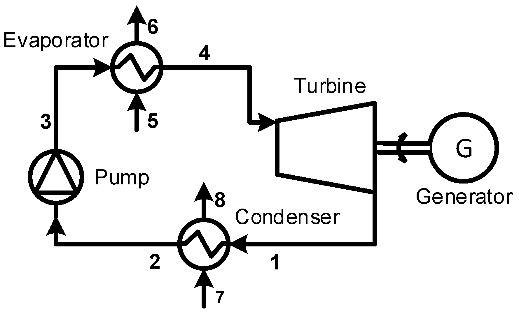
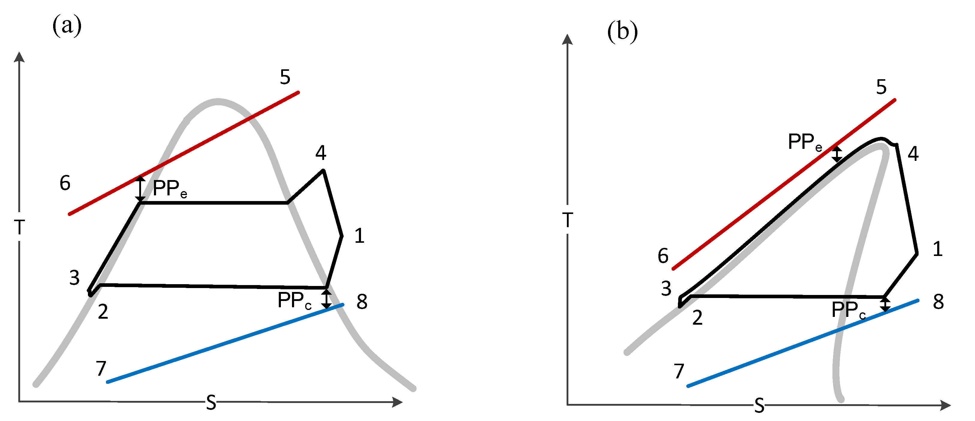
2.1. Description Subcritical and Transcritical ORC

The component diagram of the subcritical and transcritical ORC analyzed in this study is given in Figure 1. The T-s diagrams are given in Figure 2 and introduce the nomenclature used. The basic subcritical ORC consists of a pump, which pressurizes the working fluid (3), and transports it to the evaporator. In the evaporator, the working fluid is heated to the point of saturated vapor (4), cooling down the heat carrier (5–6). Next, the working fluid expands through the turbine (1) and produces mechanical work. This shaft power is then converted to electricity by the generator. The superheated working fluid at the outlet of the turbine is condensed to saturated liquid (2) in the condenser by transferring the heat to a cooling loop (7–8). The liquid working fluid is, again, pressurized by the pump (3), closing the cycle.

Figure 1. Component layout trans- and subcritical organic Rankine cycle (ORC).

Figure 1. Component layout trans- and subcritical organic Rankine cycle (ORC).

Figure 2. Temperature-entropy (T-s) diagram: (a) subcritical ORC and (b) transcritical ORC.

Figure 2. Temperature-entropy (T-s) diagram: (a) subcritical ORC and (b) transcritical ORC.

Similar to the SCORC, the TCORC consists of a pump, expander, evaporator and condenser. The working fluid is now compressed directly to supercritical pressure and heated to a supercritical state, effectively bypassing the isothermal two-phase region. Because no phase change takes place in the TCORC, the evaporator is also called a vapor generator.

2.2. Case Definition

A representative medium-temperature waste heat recovery case is considered. Exhaust gasses from an incinerator are cooled by an intermediate pressurized water loop. Part of the heat is used for heating of nearby buildings. In the original situation, the remaining heat was cooled by dry coolers. This part of the cooling loop is pressurized to 15 bar, has an outlet temperature $T_7=180$ °C and a mass flow rate of ${\dot{m}}_{hf}=15$ kg/s.

3. Model and Assumptions

3.1. Cycle Assumptions

The ORC cycle is evaluated assuming steady state conditions of all components. Pumps and turbines are characterized by their isentropic efficiency. Furthermore, heat loss to ambient is assumed negligible. An overview of the fixed parameters and variables is given in Table 3. These values are chosen based on a literature survey. In this work, conservative values are taken for the pump and turbine isentropic efficiencies. The same turbine isentropic efficiency used here is also found in the work of Wang et al. [19] and Vaja and Gambaroto [17], both consider applications on waste heat recovery. Other authors employed higher values of 0.75 [9,20] or even 0.85 [21,22]. However turbine isentropic efficiencies of 0.65 [23] are also found. The pump isentropic efficiency found in literature typically ranges between 0.6 [24,25] to 0.8 [26].

Table 3. Thermodynamic cycle parameters.

Variable	Description	Value
PPe	Pinch point temperature difference evaporator (°C)	Optimized
PPc	Pinch point temperature difference condenser (°C)	Optimized
T7	Inlet temperature cooling fluid condenser (°C)	25
T4	Inlet temperature turbine (°C)	Optimized 1
pe	Evaporation pressure (Pa)	Optimized 2
pc	Condensation pressure (Pa)	Optimized
εturbine	Isentropic efficiency turbine (-)	0.7
εpumps	Isentropic efficiency pumps (-)	0.6
εgenerator	Generator efficiency (-)	0.98
ΔTsub	Temperature subcooling (°C)	3
ΔTsup	Temperature superheating (°C)	5 2

¹ For TCORC; ² For SCORC.

Table 3. Thermodynamic cycle parameters.

Variable	Description	Value
PPe	Pinch point temperature difference evaporator (°C)	Optimized
PPc	Pinch point temperature difference condenser (°C)	Optimized
T7	Inlet temperature cooling fluid condenser (°C)	25
T4	Inlet temperature turbine (°C)	Optimized 1
pe	Evaporation pressure (Pa)	Optimized 2
pc	Condensation pressure (Pa)	Optimized
εturbine	Isentropic efficiency turbine (-)	0.7
εpumps	Isentropic efficiency pumps (-)	0.6
εgenerator	Generator efficiency (-)	0.98
ΔTsub	Temperature subcooling (°C)	3
ΔTsup	Temperature superheating (°C)	5 2

¹ For TCORC; ² For SCORC.

A certain amount of subcooling is added to better comply with real life cycles. Condensers typically have a minimal flooding. In addition, a degree of subcooling is beneficial to avoid cavitation by the working fluid pump. However, the subcooling should be maintained low to achieve a high power output. Furthermore, in an actual subcritical organic Rankine cycle design, a certain amount of superheating is included, since the control strategy is almost always based on a fixed superheating set point. Furthermore, the risk of wet vapor entering the turbine is decreased. For dry fluids, several authors [20,44,45] suggest keeping superheating low in order to increase the power output. Also, an upper pressure limit of 0.9P_crit [9,46] is imposed to avoid instable operation in the supercritical region. For the TCORC the upper pressure of the cycle is kept constant to a value of 1.12P_crit to ensure safe operation.

The pumps and turbine are modeled by their isentropic efficiency:

$${\dot{W}}_{pumps}=\frac{(h_{pump,out}-h_{pump,in)}}{{\mathrm{\epsilon }}_{pump}}{\dot{m}}_{fluid}$$

(1)

$${\dot{W}}_{turbine}=\left(h_{turbine,in}-h_{turbine,ex}\right){\mathrm{\epsilon }}_{turbine}{\dot{m}}_{wf}$$

(2)

The net power output is calculated as:

$${\dot{W}}_{net}={\dot{W}}_{turbine}-{\dot{W}}_{pump,orc}-{\dot{W}}_{pump,hf}-{\dot{W}}_{pump,cf}$$

(3)

and the thermal efficiency is defined as:

$${\mathrm{\eta }}_I=\frac{{\dot{W}}_{net}}{{\dot{Q}}_{in}}$$

(4)

with ${\dot{Q}}_{in}$ the heat input from the waste heat stream to the ORC.

3.2. Heat Exchanger Models

Both the condenser and evaporator are of the plate heat exchanger type. The model is discussed here in detail for the evaporator, but is analogous for the condenser. A distributed modeling approach is applied. The heat exchangers are divided into three zones: pre-heating, evaporating and superheating. In the pre-heating section the fluid is heated to saturated vapor, afterwards it evaporates in the evaporation section and finally superheats in the superheating section. The evaporating zone or vapor generator, in case of the TCORC, is further divided into I segments. The log mean temperature difference (LMTD) method is applied to calculate the required heat transfer area for each segment:

$${\dot{Q}}_i=\mathrm{∆}{T}_{LMTD,i}.F.U_i.A_i$$

(5)

With A the heat transfer area; F the configuration correction factor; and U the overall heat transfer coefficient:

$$\frac{1}{U_i}=\frac{1}{{\mathrm{\alpha }}_{\mathrm{hf},\mathrm{i}}}+\frac{1}{{\mathrm{\alpha }}_{\mathrm{wf},\mathrm{i}}}+\frac{t}{\mathrm{\lambda }}$$

(6)

With α the convective heat transfer coefficient; t the plate thickness; and λ the thermal conductivity of the plate. The energy balance requires that:

$${\dot{Q}}_i={\dot{m}}_{wf}\left(h_{wf,i+1}-h_{wf,i}\right)={\dot{m}}_{hf}\left(h_{hf,i+1}-h_{hf,i}\right)$$

(7)

The product of number of passes (N) and paths (K) is equal for both sides:

$$N_{ev,wf}.K_{ev,wf}=N_{ev,hf}.K_{ev,hf}$$

(8)

The pressure drop is calculated from the friction factor f:

$$\mathrm{∆}p=f\frac{L.G_{eq}^2}{D_h.{\mathrm{\rho }}_l}$$

(9)

With L the channel length of the heat exchanger and $G_{eq}$ the equivalent mass flux:

$$G_{eq}=G\left[1-x+x{\left(\frac{{\mathrm{\rho }}_l}{{\mathrm{\rho }}_g}\right)}^{\left(1/2\right)}\right]$$

(10)

For the single phase, the well-known convective heat transfer and pressure drop correlations of Martin [47] are used. For the two-phase evaporation process, the pressure drop and convective heat transfer correlations of Han et al. [48] are implemented:

$$N{u}_e=G{e}_{1,e}R{e}_{eq}^{Ge2,e}B{o}_{eq}^{0.3}P{r}^{0.4}$$

(11)

$$f_e=G{e}_{3,e}R{e}_{eq}^{Ge4,e}$$

(12)

with

$$G{e}_{1,e}=2.81{\left(p_{co}/D_h\right)}^{-0.041}{\left(\mathrm{\pi }/2-\mathrm{\beta }\right)}^{-2.83}$$

(13)

$$G{e}_{2,e}=0.746{\left(p_{co}/D_h\right)}^{-0.082}{\left(\mathrm{\pi }/2-\mathrm{\beta }\right)}^{0.61}$$

(14)

$$G{e}_{3,e}=64,710{\left(p_{co}/D_h\right)}^{-5.27}{\left(\mathrm{\pi }/2-\mathrm{\beta }\right)}^{-3.03}$$

(15)

$$G{e}_{4,e}=-1.314{\left(p_{co}/D_h\right)}^{-0.062}{\left(\mathrm{\pi }/2-\mathrm{\beta }\right)}^{-0.47}$$

(16)

These equations were derived from experimental measurements with $G_{wf}=13-34$ kg/m²/s; $\dot{q}=2.5-8.5$ kW/m²; $x=0-0.95$ and chevron angles 20°, 35° and 45°.

For the two-phase condensation process the following equations by Han et al. [49] are used:

$$N{u}_c=G{e}_{1,c}R{e}_{eq}^{Ge2,c}P{r}^{1/3}$$

(17)

$$f_e=G{e}_{3,c}R{e}_{eq}^{Ge4,c}$$

(18)

with

$$G{e}_{1,c}=11.2{\left(p_{co}/D_h\right)}^{-2.83}{\left(\mathrm{\pi }/2-\mathrm{\beta }\right)}^{-4.5}$$

(19)

$$G{e}_{2,c}=0.746{\left(p_{co}/D_h\right)}^{-0.23}{\left(\mathrm{\pi }/2-\mathrm{\beta }\right)}^{1.48}$$

(20)

$$G{e}_{3,c}=64,710{\left(p_{co}/D_h\right)}^{4.17}{\left(\mathrm{\pi }/2-\mathrm{\beta }\right)}^{-7.75}$$

(21)

$$G{e}_{4,c}=-1.314{\left(p_{co}/D_h\right)}^{0.0925}{\left(\mathrm{\pi }/2-\mathrm{\beta }\right)}^{-1.3}$$

(22)

These equations were derived from experimental measurements with $G_{wf}=13-34$ kg/m²/s; $\dot{q}=4.7-5.3$ kW/m²; $x=0.15-0.95$ and chevron angles 20°, 35° and 45°.

The equivalent Reynolds number ($R{e}_{eq}$) and boiling number ($B{o}_{eq}$) are defined as:

$$R{e}_{eq}=\frac{G_{eq}{D}_h}{{\mathrm{\mu }}_l}$$

(23)

$$B{o}_{eq}=\frac{\dot{q}}{G_{eq}{h}_{lg}}$$

(24)

The correlations by Han et al. [48,49] can be applied in the range $R{e}_{eq}$ from 300 to 4000. When compared to the Hsieh and Lin correlation [50], the Nusselt numbers are very similar. In comparison with the Yan and Lin correlation [51], which is valid for higher Reynolds numbers, extrapolation gives Nusselt numbers that are lower. In general, the implemented boiling and condensation heat transfer correlations give rather conservative values. While the above dimensionless correlations were derived for R410A they are frequently used to design heat exchangers using R245fa [38,52,53]. However, there is clearly a need for high accuracy heat transfer and pressure drop correlations specifically made for contemporary ORC working fluids. A detailed comparison of boiling and condensation heat transfer correlations can be found in the work of García-Cascales et al. [54].

Both Cayer et al. [27] as well as Shenghjun et al. [28] used the Petukhov-Kranoschekov [55] correlations to calculate the convective heat transfer coefficient and pressure drop in the supercritical state. The same correlation is used here for simulations of the TCORC:

$$Nu=N{u}_0{\left(\frac{{\mathrm{\mu }}_b}{{\mathrm{\mu }}_{wl}}\right)}^{0.11}{\left(\frac{k_b}{k_{wl}}\right)}^{-0.33}{\left(\frac{{\overline{c}}_p}{c_{p,b}}\right)}^{0.35}$$

(25)

$$N{u}_0=\frac{\left(\frac{f}{8}\right)R{e}_{b}Pr}{12.7\sqrt{\frac{f}{8}\left(P{r}^{2/3}-1\right)+1.07}}$$

(26)

$$f={\left(1.82{\log }_{10}R{e}_b-1.64\right)}^{-2}$$

(27)

In the SCORC, the evaporating zone is divided in I = 20 segments, while in the case of the TCORC, the vapor generator is segmented in I = 60 segments. For these values, the net power output changes less than 0.1% when doubling the number of segments. Thus, to keep an acceptable calculation time, these values are used throughout this work. The fixed values to model the plate heat exchanger are given in Table 4. The values reported in Table 4 are generally accepted values for the design of plate heat exchangers [16,29,38,56,57]. With plate heat exchangers, the range of these parameters are greatly restricted due to manufacturing limitations [56]. The plate thickness is typically between 0.4 and 1.2 mm and the corrugation depth between 1.5 and 5.4 mm. These limitations therefore constrain the optimization potential. Further optimization [58] is still possible by varying the corrugation angle [53]. In this work it was chosen to compare different cycles using identical assumptions on the plate heat exchanger geometry.

Table 4. Design parameters plate heat exchangers.

Variable	Description	Value
$D_h$	Hydraulic diameter (m)	0.0035
$t$	Plate thickness (m)	0.0005
$\mathrm{\beta }$	Chevron angle (°)	45
$\mathrm{\lambda }$	Plate thermal conductivity (W/m/K)	13.56
$p_{co}$	Corrugation pitch (m)	0.007

Table 4. Design parameters plate heat exchangers.

Variable	Description	Value
$D_h$	Hydraulic diameter (m)	0.0035
$t$	Plate thickness (m)	0.0005
$\mathrm{\beta }$	Chevron angle (°)	45
$\mathrm{\lambda }$	Plate thermal conductivity (W/m/K)	13.56
$p_{co}$	Corrugation pitch (m)	0.007

3.3. Cost Models

The cost correlations are based on the exponential scaling law and are taken from Turton et al. [59]. Cost estimates performed with equipment cost correlations are classified as “preliminary” or “study” estimates, which gives accuracies in the range of +40% to −25% [59]. Data, from a survey of manufacturers during the period of May 2001 to September 2001, was fitted to the following correlation:

$${\log }_{10}\left(C_{PEC}^0\right)=K_1+K_2{\log }_{10}\left(B\right)+K_3\cdot {({\log }_{10}B)}^2$$

(28)

B is the capacity or size parameter, K1, K2 and K3 are parameters of the curve fitting. For heat exchangers, B corresponds to the heat transfer area, while for pumps and turbines this corresponds with, respectively, the power input and output. These correlations were derived for a general Chemical Engineering Plant Cost Index (CPCI) of 397. To actualize the cost, a multiplication with (CPCI₂₀₀₁/CPCI₂₀₁₃) is made. The CPCI₂₀₁₃ is set to the value of August 2013 (564.7). The cost functions are provided in US dollars. To convert the values to euros, a conversion factor of 0.731 (19 December 2013) is taken into account. Correction factors $F_p$ and $F_m$ take into account the operating pressure and type of material used. $F_p$ is calculated by:

$${\log }_{10}(F_p)=C_1+C_2{\log }_{10}p+C_3\cdot {({\log }_{10}p)}^2$$

(29)

The coefficients for the different components are given in Table 5 and Table 6. The bare module cost takes into account direct (installation of equipment, piping, instrumentation and controls) and indirect costs (engineering and supervision, transportation):

$$C_{BM}=C_{PEC}^0{F}_{BM}$$

(30)

with $F_{BM}$ the bare module factor:

$$F_{BM}=B_1+B_2{F}_p{F}_m$$

(31)

Table 5. Cost parameters [59].

Component	B	K1	K2	K3	Valid Range
Plate heat exchangers	Area (m2)	4.6656	−0.1557	0.1547	10–1000 (m2)
Turbine	Fluid power (kW)	2.2476	1.4965	−0.1618	100–1500 (kW)
Pumps (centrifugal)	Shaft power (kW)	3.3892	0.0536	0.1538	1–300 (kW)
Electrical motor pump	Shaft power (kW)	2.4604	1.4191	−0.1798	75–2600 (kW)
Electrical generator [41]	Shaft power (kW)	$C_{PEC}^0=1850000·{\left(P/11800\right)}^{0.94}$

Table 5. Cost parameters [59].

Component	B	K1	K2	K3	Valid Range
Plate heat exchangers	Area (m2)	4.6656	−0.1557	0.1547	10–1000 (m2)
Turbine	Fluid power (kW)	2.2476	1.4965	−0.1618	100–1500 (kW)
Pumps (centrifugal)	Shaft power (kW)	3.3892	0.0536	0.1538	1–300 (kW)
Electrical motor pump	Shaft power (kW)	2.4604	1.4191	−0.1798	75–2600 (kW)
Electrical generator [41]	Shaft power (kW)	$C_{PEC}^0=1850000·{\left(P/11800\right)}^{0.94}$

Table 6. Pressure factor, material factor and bare module cost [59].

Component	B1	B2	C1	C2	C3	Fm	FBM
Plate heat exchangers p (bar) < 19	0.96	1.21	0	0	0	1	-
Turbine	-	-	-	-	-	-	3.5
Pumps (centrifugal) 10 < p (bar) < 100	1.89	1.35	−0.3935	0.3957	−0.00226	1	-
Pumps (centrifugal) p (bar) < 10	1.89	1.35	0	0	0	1	-
Electrical motor pump	-	-	-	-	-	-	1.5
Electrical generator [41]	-	-	-	-	-	-	1.5

Table 6. Pressure factor, material factor and bare module cost [59].

Component	B1	B2	C1	C2	C3	Fm	FBM
Plate heat exchangers p (bar) < 19	0.96	1.21	0	0	0	1	-
Turbine	-	-	-	-	-	-	3.5
Pumps (centrifugal) 10 < p (bar) < 100	1.89	1.35	−0.3935	0.3957	−0.00226	1	-
Pumps (centrifugal) p (bar) < 10	1.89	1.35	0	0	0	1	-
Electrical motor pump	-	-	-	-	-	-	1.5
Electrical generator [41]	-	-	-	-	-	-	1.5

For some components, the bare module factor is directly given. The total module cost, additionally, includes contingency costs and fees, here taken as, respectively, 15% and 3%, according to Turton et al. [59]:

$$C_{TM}=1.18(C_{BM,c}+C_{BM,e}+C_{BM,turbine}+C_{BM,pump,wf}+C_{BM,pump,hf}+C_{BM,pump,cf}+C_{BM,motor,wf}+C_{BM,motor,cf}+C_{BM,motor,hf}+C_{BM,generator})$$

(32)

The grass root cost includes the costs for construction and site preparation. These costs are highly dependent on the specific site; here the proposed values by Turton et al. [59] were followed:

$$C_{GR}=C_{TM}+0.5{\displaystyle \sum }_{components}{C}_{BM}^0$$

(33)

${\mathrm{C}}_{\mathrm{BM}}^0$ is the bare module cost at base conditions ($F_p$ = 1, $F_m$ = 1). The specific investment cost (SIC) is in this work defined as:

$$SIC=\frac{C_{GR}}{{\dot{W}}_{net}}$$

(34)

3.4. Working Fluid Selection

The working fluid selected in this work must be able to give an acceptable expander design, which can comply with the isentropic efficiency imposed. Therefore, R245fa is taken as reference working fluid for the SCORC and TCORC due to its de facto standard use in commercial ORC installations [2,24]. Furthermore, R245fa has proven itself for various expander designs, either volumetric [60,61] or turbine [62,63,64,65] technology. The selected working fluid is not necessarily optimal for the discussed cycles, but provides a good benchmark for further study and comparison.

The thermophysical data is taken from Engineering Equation Solver (EES) [66]. EES implements the fundamental equations of state for R245fa presented by Lemmon and Span [67]. These correlations were derived in view of advanced technical applications for which very low uncertainties are not required [67]. The same fundamental equations of state are found in REFPROP 9.1 [68]. Uncertainty data is provided in Table 7. In EES, the transport properties were obtained from the documentation provided by Honeywell. There is no information available on the uncertainty of these correlations. As such, caution should be taken when using EES for the final design iteration. In REFPROP 9.1 [68], the viscosity and thermal conductivity are, respectively, derived from a correlation proposed by Huber et al. [69] and Marsh et al. [70] and uncertainty information is given.

Table 7. Uncertainty for R245fa fundamental equation of state [67].

Variable	Uncertainty
Density	0.1% (liquid phase, temperature <400 K and pressure <30 MPa) 0.2% (liquid phase, temperature >310 K and pressure >30 MPa) 1% (liquid phase, temperature <310 K and pressure >30 MPa) 1% (vapor phase, temperature >400 K)
Vapor pressure	0.2% (temperature >250 K) 0.35% (temperature >370 K)
Liquid phase heat capacity	5%

Table 7. Uncertainty for R245fa fundamental equation of state [67].

Variable	Uncertainty
Density	0.1% (liquid phase, temperature <400 K and pressure <30 MPa) 0.2% (liquid phase, temperature >310 K and pressure >30 MPa) 1% (liquid phase, temperature <310 K and pressure >30 MPa) 1% (vapor phase, temperature >400 K)
Vapor pressure	0.2% (temperature >250 K) 0.35% (temperature >370 K)
Liquid phase heat capacity	5%

3.5. Expander Considerations

To assess the feasibility of the fixed turbine isentropic efficiency given in Table 3, two expander evaluation criteria are introduced: the size parameter (SP) and the volume ratio (VR).

$$SP=\frac{{{\dot{V}}_{turbine,in}}^{0.5}}{\mathrm{∆}{h_{isentropic}}^{0.25}}$$

(35)

$$VR=\frac{{\dot{v}}_{turbine,out}}{{\dot{v}}_{turbine,in}}$$

(36)

General design ranges can be associated to both expander evaluation criteria. The SP directly correlates with the size of the expander and typically varies between 0.02 and 1 m [71,72]. For SP values between 0.2 and 1 m the change in isentropic efficiency is small [71]. A lower SP results in higher losses associated to the relative increase in clearances and roughness. In contrast, a low VR results in higher isentropic efficiencies. Volume ratios lower than 50 are needed to get isentropic efficiencies in the range of 0.7 to 0.8 [71].

4. Optimization Strategy

A multi-objective optimization scheme with the optimization variables from Table 8 is set up. The number of passes always relates to the side with the lowest mass flow rate in order to balance pressure drops and heat transfer coefficients [73]. The limits used have been chosen based on values found in literature [33,38,57]. The value range is chosen wide enough in order not to constrain the optimization around the point of minimum SIC. The variables in the optimization process affect the sizing and the power output of the cycle. They are however not directly constrained by manufacturing limitations. Manufacturing constraints are taken into account, as discussed above, trough the careful choice of parameters from Table 3 and Table 4.

Table 8. Decision variables and their range.

Variable	Description	Lower	Upper
$G_{\mathrm{c},\mathrm{wf}}$	Mass flux working fluid condenser (kg/m2/s)	20	100
$G_{\mathrm{e},\mathrm{wf}}$	Mass flux working fluid evaporator (kg/m2/s)	20, 100 1	50, 200 1
$P{P}_{\mathrm{c}}$	Pinch point temperature difference condenser (°C)	3	10
$P{P}_e$	Pinch point temperature difference evaporator (°C)	3	10
$T_c$	Liquid saturation temperature condenser (°C)	35	50
$T_e$ 2	Liquid saturation temperature evaporator (°C)	100	148.5
T71	Turbine inlet temperature (°C)	150	175
$N_e$	Number of passes hot fluid side evaporator (-)	1	3
$N_c$	Number of passes cold fluid side condenser (-)	1	3

¹ for TCORC; ² for SCORC.

Table 8. Decision variables and their range.

Variable	Description	Lower	Upper
$G_{\mathrm{c},\mathrm{wf}}$	Mass flux working fluid condenser (kg/m2/s)	20	100
$G_{\mathrm{e},\mathrm{wf}}$	Mass flux working fluid evaporator (kg/m2/s)	20, 100 1	50, 200 1
$P{P}_{\mathrm{c}}$	Pinch point temperature difference condenser (°C)	3	10
$P{P}_e$	Pinch point temperature difference evaporator (°C)	3	10
$T_c$	Liquid saturation temperature condenser (°C)	35	50
$T_e$ 2	Liquid saturation temperature evaporator (°C)	100	148.5
T71	Turbine inlet temperature (°C)	150	175
$N_e$	Number of passes hot fluid side evaporator (-)	1	3
$N_c$	Number of passes cold fluid side condenser (-)	1	3

¹ for TCORC; ² for SCORC.

A genetic algorithm optimizes two objective functions simultaneously. In this work this is ${\dot{W}}_{net}$ and $C_{inv}$. The benefit of working with a genetic algorithm includes searching for the global optimum while avoiding complex derivatives. An initial population of parameters is generated in the search area. The solutions are afterwards assessed, based on the objective criteria. The fittest are selected to construct a new population based on crossover and mutation operations [43].

The Non-dominated Sorting Genetic Algorithm II (NSGA-II) was used in this work [43,74]. The parameter settings of the genetic algorithm are provided in Table 9. A population of 120 can be considered a good default value for this type of optimization. In other works, population sizes of 40 [75], 30 [30,31], 100 [76,77] and 150 [78] are employed. A population size of 200 was also considered, but the changes on the Pareto front were marginal at the cost of doubling the calculation time. The optimization was done in MATLAB [79] with the EES [66] models coupled by the Dynamic Data Exchange (DDE) protocol. Under the given parameters and assumptions the calculation time is approximately six hours on an E5-2736 v2 Intel processor. Due to limitations of the DDE protocol, only a single core could be used.

Table 9. Parameter settings of the genetic algorithm.

Parameter	Value
Generations	50
Population size	120
Crossover rate	0.8
Migration rate	0.2
Mutation type	Gaussian (shrink = 1, scale = 1)

Table 9. Parameter settings of the genetic algorithm.

Parameter	Value
Generations	50
Population size	120
Crossover rate	0.8
Migration rate	0.2
Mutation type	Gaussian (shrink = 1, scale = 1)

5. Results and Discussion

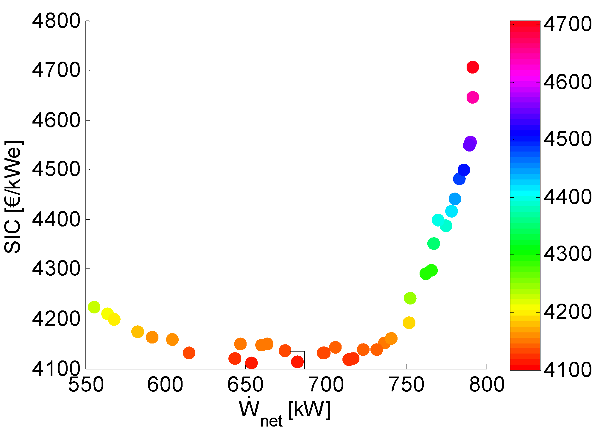
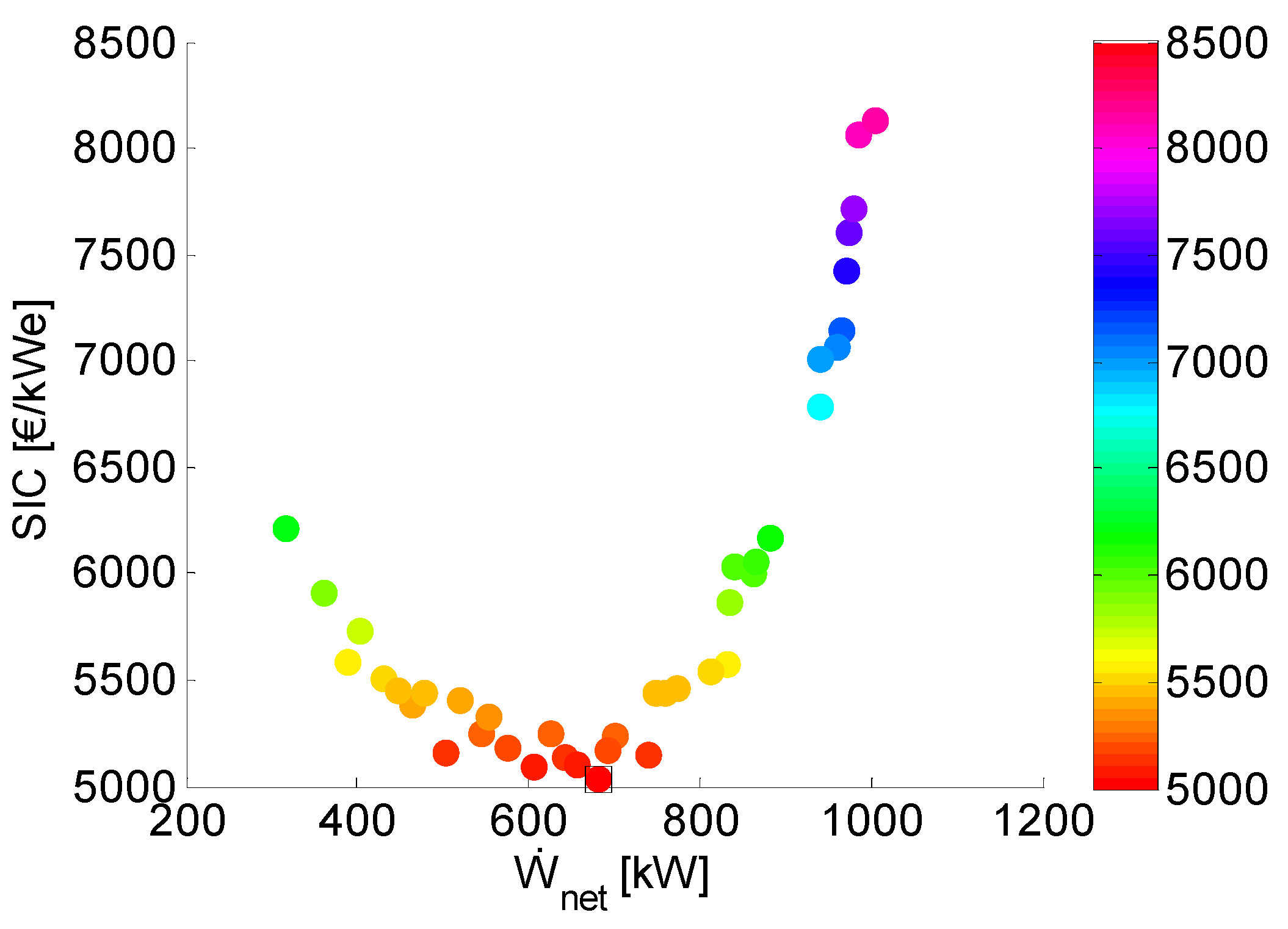
5.1. Pareto Fronts and Specific Investment Cost

The resulting Pareto fronts of the SIC in function of the net power output are plotted in Figure 3 and Figure 4 for, respectively, the SCORC and TCORC. The approximate point of minimum SIC is visualized by a black rectangle. This black rectangle is also shown in Figure 4 to Figure 12. The corresponding optimized design parameters for the point of minimum SIC are given in Table 10. ${\dot{W}}_{net,SIC}$ is the net power output corresponding with the point of minimum SIC.

Table 10. Results of minimum specific investment cost (SIC) and maximum net power output (${\dot{W}}_{net}$).

Variable	Minimum SIC		Maximum Net Power Output
	SCORC	TCORC	SCORC	TCORC
${\dot{W}}_{net}$ (kWe)	681.8	681.3	791.5	1040
${\mathrm{\eta }}_I$ (%)	10.47	11.20	10.9	11.1
$P{P}_{\mathrm{e}}$ (°C)	5.9	8.2	3	3
$P{P}_c$ (°C)	8.0	7.0	3	3
$T_e$ (°C)	128.8	-	124.5	-
$T_c$ (°C)	41.1	39.85	35.2	37.0
$T_4$ (°C)	128.8	161.6	124.5	160.0
$C_{GR}$ (k€)	2805	3436	3725	8162
$SIC$ (€/kWe)	4114	5044	4707	8137
$A_e$ (m2)	258	879	418	1205
$A_c$ (m2)	398	385	888	756
$N_e$ (-)	2	2	2	2
$N_c$ (-)	2	2	2	2
${\dot{m}}_{e,hf}$ (kg/s)	28.58	26.7	28.9	40.52
${\dot{m}}_{e,cf}$ (kg/s)	205.30	150	217	255
$G_{e,wf}$ (kg/s/m2)	91.0	187	70.3	175.0
$G_{c,wf}$ (kg/s/m2)	54.0	53.5	22.4	46.1

Table 10. Results of minimum specific investment cost (SIC) and maximum net power output (${\dot{W}}_{net}$).

Variable	Minimum SIC		Maximum Net Power Output
	SCORC	TCORC	SCORC	TCORC
${\dot{W}}_{net}$ (kWe)	681.8	681.3	791.5	1040
${\mathrm{\eta }}_I$ (%)	10.47	11.20	10.9	11.1
$P{P}_{\mathrm{e}}$ (°C)	5.9	8.2	3	3
$P{P}_c$ (°C)	8.0	7.0	3	3
$T_e$ (°C)	128.8	-	124.5	-
$T_c$ (°C)	41.1	39.85	35.2	37.0
$T_4$ (°C)	128.8	161.6	124.5	160.0
$C_{GR}$ (k€)	2805	3436	3725	8162
$SIC$ (€/kWe)	4114	5044	4707	8137
$A_e$ (m2)	258	879	418	1205
$A_c$ (m2)	398	385	888	756
$N_e$ (-)	2	2	2	2
$N_c$ (-)	2	2	2	2
${\dot{m}}_{e,hf}$ (kg/s)	28.58	26.7	28.9	40.52
${\dot{m}}_{e,cf}$ (kg/s)	205.30	150	217	255
$G_{e,wf}$ (kg/s/m2)	91.0	187	70.3	175.0
$G_{c,wf}$ (kg/s/m2)	54.0	53.5	22.4	46.1

Figure 3. Pareto front SIC vs. net power output (${\dot{W}}_{net}$) for the subcritical organic Rankine cycle (SCORC).

Figure 3. Pareto front SIC vs. net power output (${\dot{W}}_{net}$) for the subcritical organic Rankine cycle (SCORC).

Figure 4. Pareto front SIC vs. net power output (${\dot{W}}_{net}$) for the transcritical organic Rankine cycle (TCORC).

Figure 4. Pareto front SIC vs. net power output (${\dot{W}}_{net}$) for the transcritical organic Rankine cycle (TCORC).

Figure 5. (a) Pinch point temperature difference evaporator ($P{P}_e$) and (b) pinch point temperature difference condenser ($P{P}_c$) in function of SIC for the SCORC.

Figure 5. (a) Pinch point temperature difference evaporator ($P{P}_e$) and (b) pinch point temperature difference condenser ($P{P}_c$) in function of SIC for the SCORC.

Figure 6. (a) $P{P}_e$ and (b) $P{P}_c$ in function of net power output (${\dot{W}}_{net}$) for the SCORC.

Figure 6. (a) $P{P}_e$ and (b) $P{P}_c$ in function of net power output (${\dot{W}}_{net}$) for the SCORC.

Figure 7. (a) Evaporation temperature ($T_e$) and (b) condensation temperature ($T_c$) in function of SIC for the SCORC.

Figure 7. (a) Evaporation temperature ($T_e$) and (b) condensation temperature ($T_c$) in function of SIC for the SCORC.

Figure 8. (a) Mass flux evaporator ($G_e$) and (b) mass flux condenser ($G_c$) in function of SIC for the SCORC.

Figure 8. (a) Mass flux evaporator ($G_e$) and (b) mass flux condenser ($G_c$) in function of SIC for the SCORC.

Figure 9. (a) $P{P}_e$ and (b) $P{P}_c$ in function of SIC for the TCORC.

Figure 9. (a) $P{P}_e$ and (b) $P{P}_c$ in function of SIC for the TCORC.

Figure 10. (a) $P{P}_e$ and (b) $P{P}_c$ in function of ${\dot{W}}_{net}$ for the TCORC.

Figure 10. (a) $P{P}_e$ and (b) $P{P}_c$ in function of ${\dot{W}}_{net}$ for the TCORC.

Figure 11. (a) $T_4$ and (b) $T_c$ in function of SIC for the TCORC.

Figure 11. (a) $T_4$ and (b) $T_c$ in function of SIC for the TCORC.

Figure 12. (a) $G_e$ and (b) $G_c$ in function of SIC for the TCORC.

Figure 12. (a) $G_e$ and (b) $G_c$ in function of SIC for the TCORC.

It is clear that around ${\dot{W}}_{net,SIC}$, the SIC is not very sensitive to the net power output generated by the system and this for both the SCORC and TCORC. For increasing ${\dot{W}}_{net}$, the SIC rises sharply for both the SCORC (${\dot{W}}_{net}$ = 782.9 kW, SIC = 4482 €/kWe) and TCORC (${\dot{W}}_{net}$ = 771.6 kW, SIC = 5463 €/kWe). While for decreasing ${\dot{W}}_{net}$, the SIC increases only gradually for both the SCORC (${\dot{W}}_{net}$ = 582.5 kW, SIC = 4176 €/kWe) and TCORC (${\dot{W}}_{net}$ = 574 kW, SIC = 5187 €/kWe). The physical explanation is given in the Section 5.2 by investigating the resulting parameter space from the optimization.

The point of ${\dot{W}}_{net,SIC}$ is almost equal for both cycles. In this point, the TCORC has a higher thermal efficiency, but also an increased heat transfer area for the vapor generator. The result is an increase in SIC of 22%. Interesting to note is that the resulting optimization of the condenser side is almost identical for both cycles.

Furthermore, the TCORC has the benefit of achieving higher net power output when solely optimizing for maximum power output (${\dot{W}}_{net,max}$), see Table 10. As expected the maximum power output is found for the lower boundary on the pinch point temperature difference. However, this is not necessarily true for the condensation temperature as the auxiliary power for pumping the cooling fluid is taken into account. The maximum power output of the TCORC amounts to 1040 kW compared to 791.5 kW for the SCORC. This is a power increase up to 31.5%. However, this also comes with an increased SIC of 72.8%.

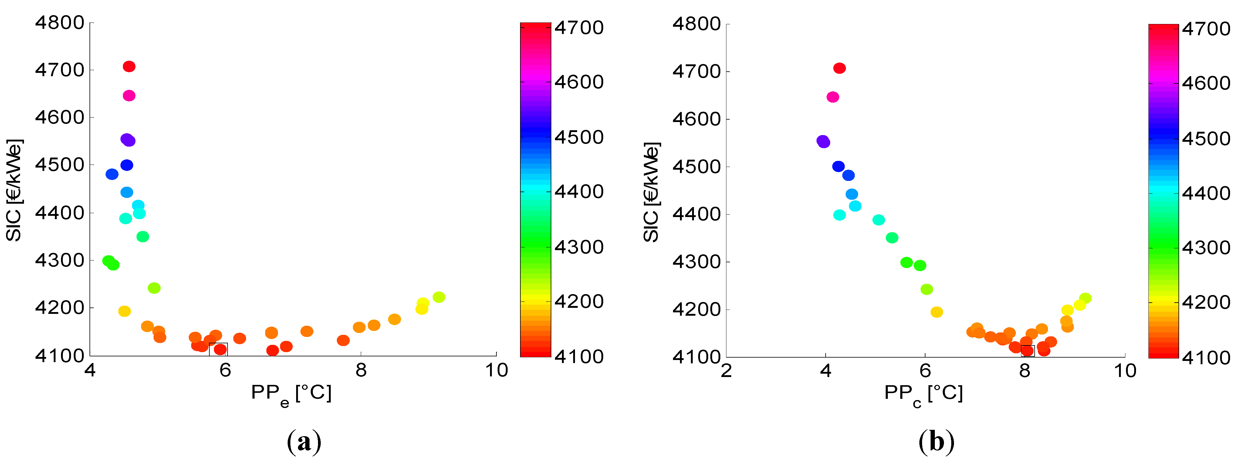
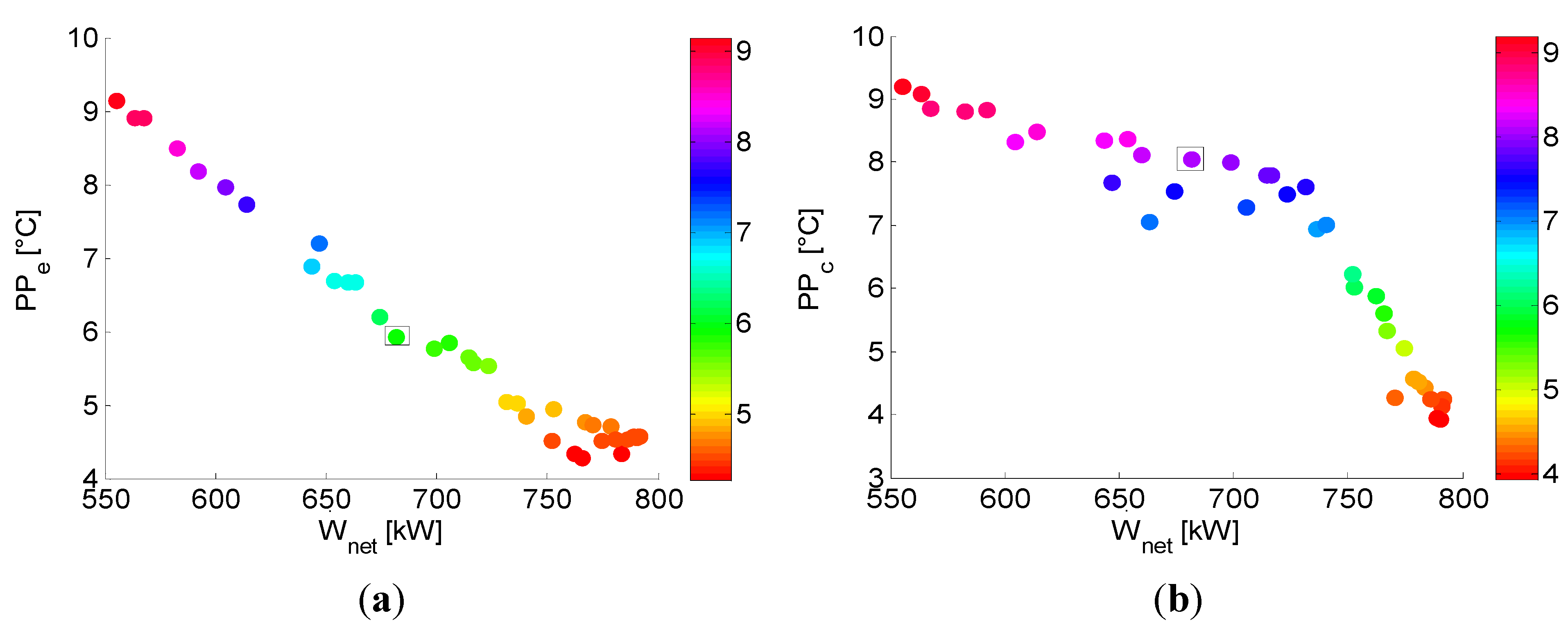
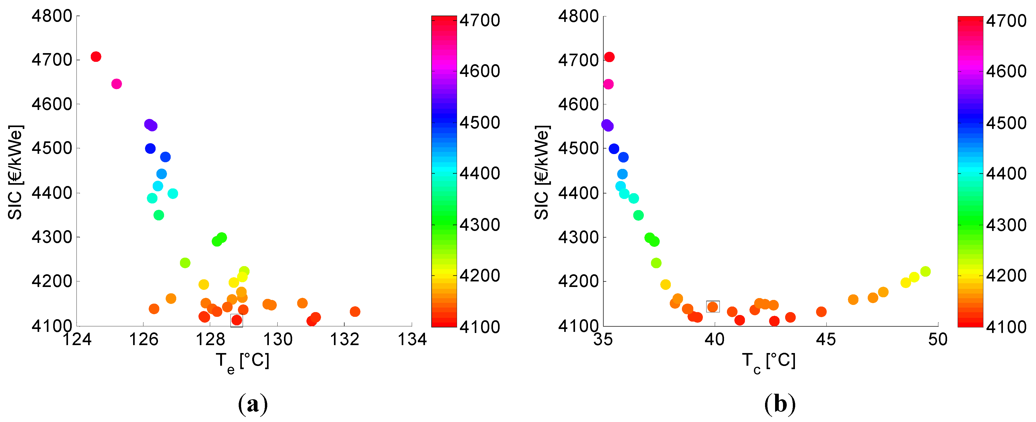
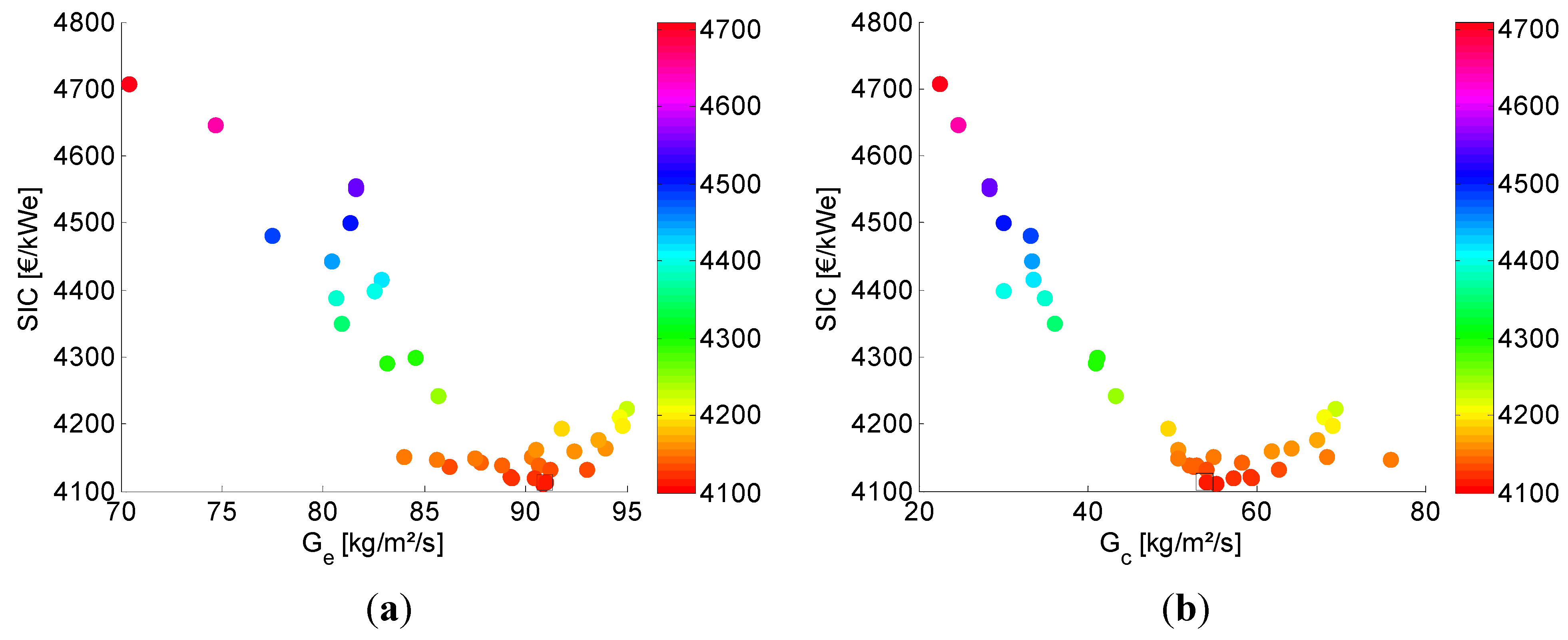
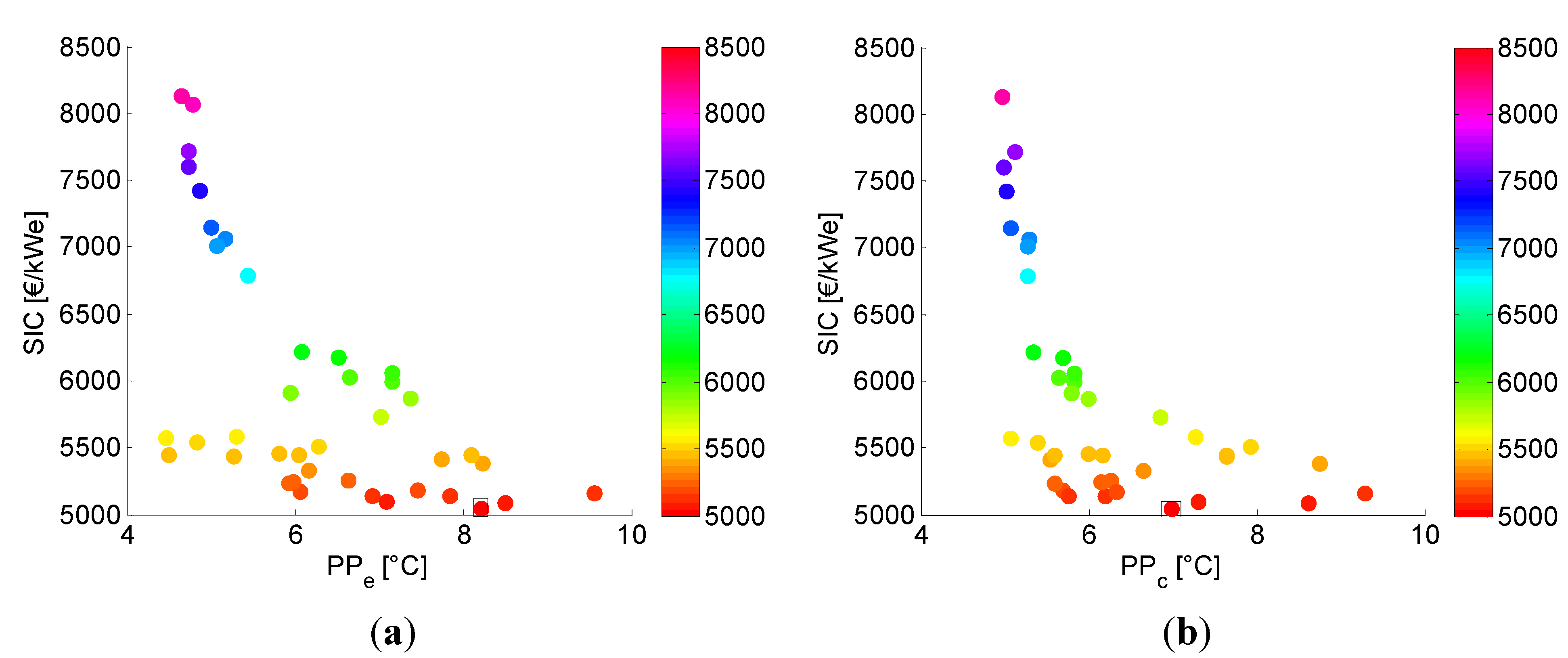
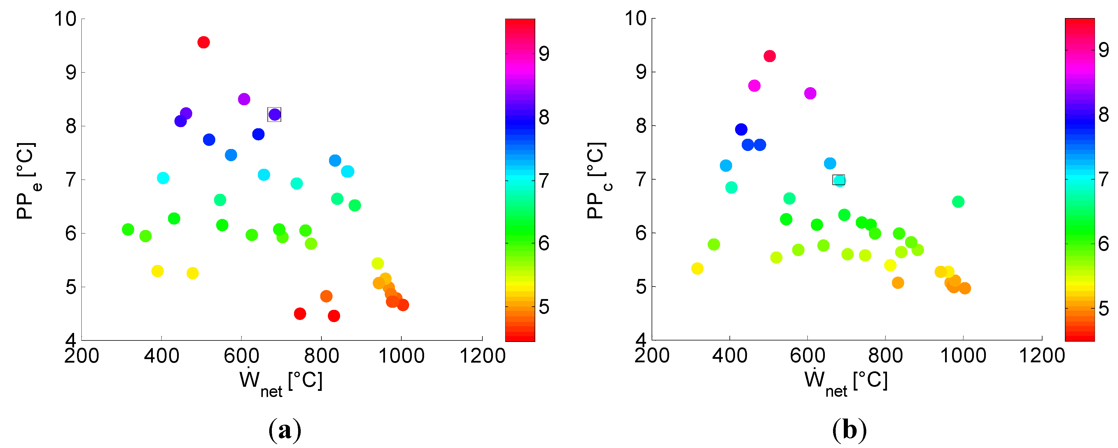
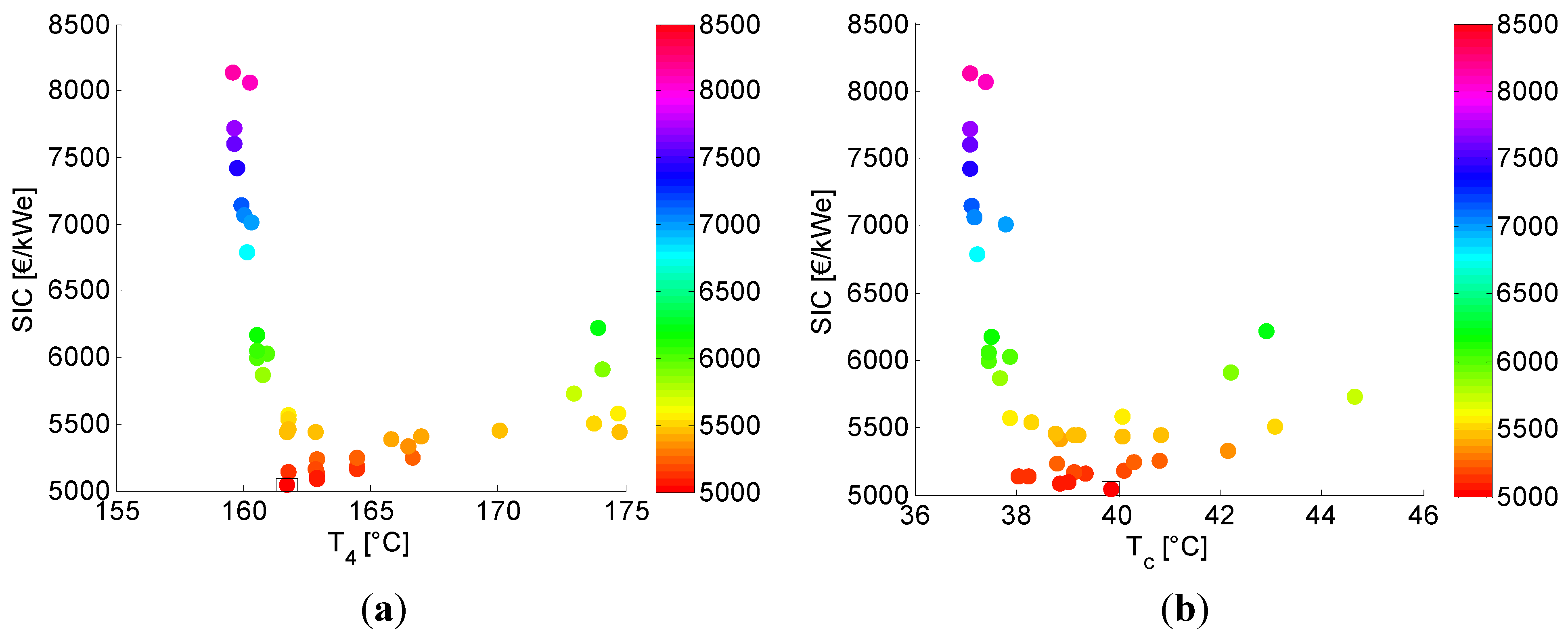
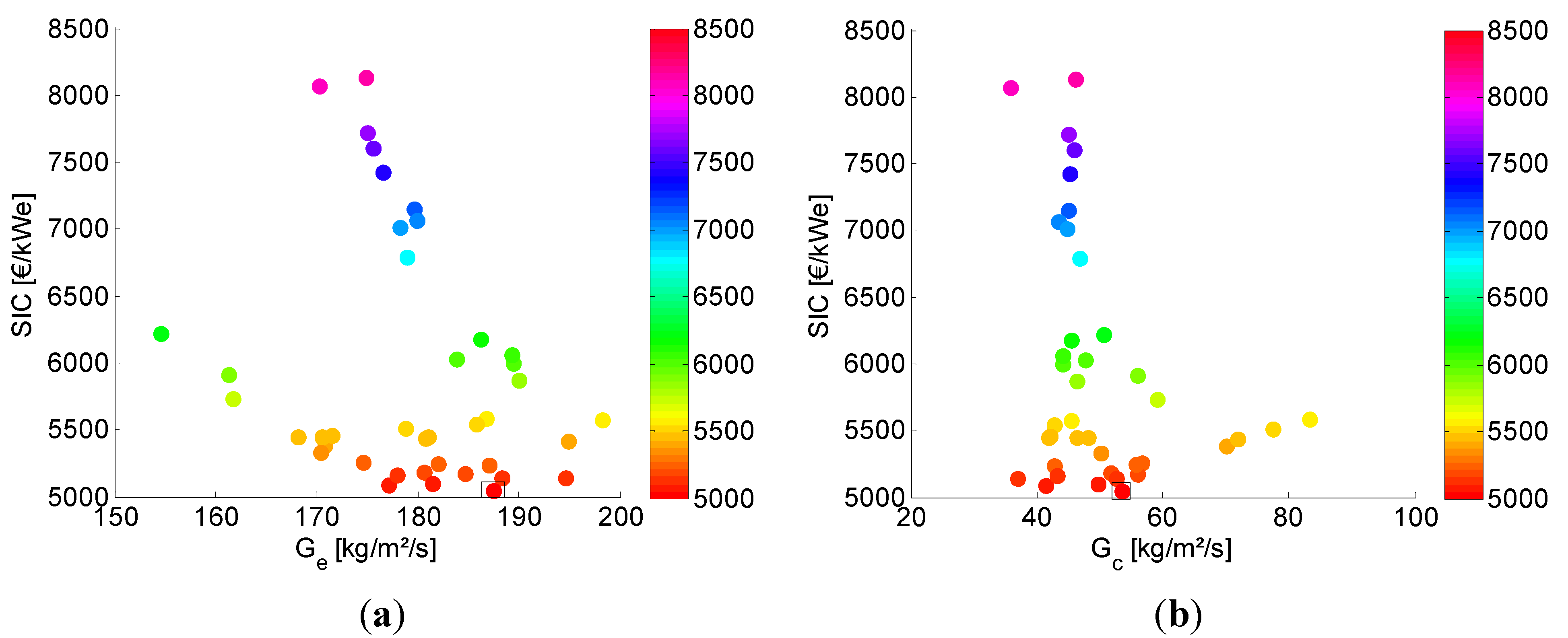
5.2. Analysis of the Parameter Space

In this paragraph, the parameter space resulting from the multi-objective optimization is analyzed. First the SCORC is discussed followed by the TCORC.

The effect of the pinch point temperature difference on the SCORC is visualized in Figure 5. Around the point of minimum SIC the pinch point temperature difference of the evaporator $P{P}_e$ is relatively constant. However, the SIC increases sharply when the $P{P}_e$ drops below 5 °C. This is explained by the large increase in heat surface area of the evaporator and the major share of the evaporator cost (which is discussed in Section 5.3). Furthermore, a decrease in $P{P}_e$ directly results in a higher net power output, see Figure 6a. This also explains the sharp increase in investment cost seen in Figure 4. The pinch point temperature difference of the condenser $P{P}_c$ is almost constant around the point of minimum SIC. For the condenser the sharp increase in SIC is noticeable starting from $P{P}_c$ = 4 °C. From Figure 6b follows that for increasing power output after the point ${\dot{W}}_{net}$ = 740 kW it is necessary to drastically decrease $P{P}_c$. Before, this parameter was maintained almost unchanged. This indicates that from ${\dot{W}}_{net}$ = 740 kW a decreased $P{P}_c$ leads to a power increase with the lowest associated cost compared to the other optimization parameters.

The effect of the evaporation temperature and condensation temperature is shown in Figure 7. Between $T_e$ = 126.3 °C ($\mathrm{SIC}$ = 4139 €/kWh) and $T_e$ = 132.3 ($\mathrm{SIC}$ = 4132 €/kWh) the variation on the SIC is marginal, see Figure 7a. Indicating that $T_e$ is not a sensitive factor in the optimization process. In contrast, for $T_c$ there is a clear extreme visible at $T_c$ = 40 °C. Deviations around this point have a significant effect on the SIC. For changes in $T_c$, not only the required heat transfer surface changes, but also the required cooling water flow rate and thus auxiliary power.

The effect of mass flux variation is visualized in Figure 8. The mass flux essentially determines the balance between pressure drop in the heat exchanger and the heat transfer coefficient. Again, there are distinct extremes visible around $G_e$ = 90.8 kg/m²/s and $G_c$ = 54.0 kg/m²/s.

Overall, the results of the optimization imply a large dependency between the parameters mutually and their objective functions. Furthermore, different parameters become dominant depending on the investigated point on the Pareto front.

Analogous figures are made for the TCORC. In Figure 9 the effect of $P{P}_e$ and $P{P}_c$ on the SIC is shown for the TCORC. The clear relation found for the SCORC is not observed here. Low pinch points can lead to high specific investment costs but this is clearly not the dominant parameter in the optimization. The effect of a low PP on the SIC can plainly be offset by changing other parameters. The same trend is visible in Figure 10 for $P{P}_e$ and $P{P}_c$ in function of ${\dot{W}}_{net}$. The dominant factor in the optimization is the maximum temperature $T_4$ in the cycle and the condensation temperature $T_c$. Both show clear extrema in function of the SIC as shown in Figure 11. For the mass flux rate, see Figure 12, a low SIC can be found between $G_e$ = 170–195 kg/m²/s and $G_c$ = 37–57 kg/m²/s.

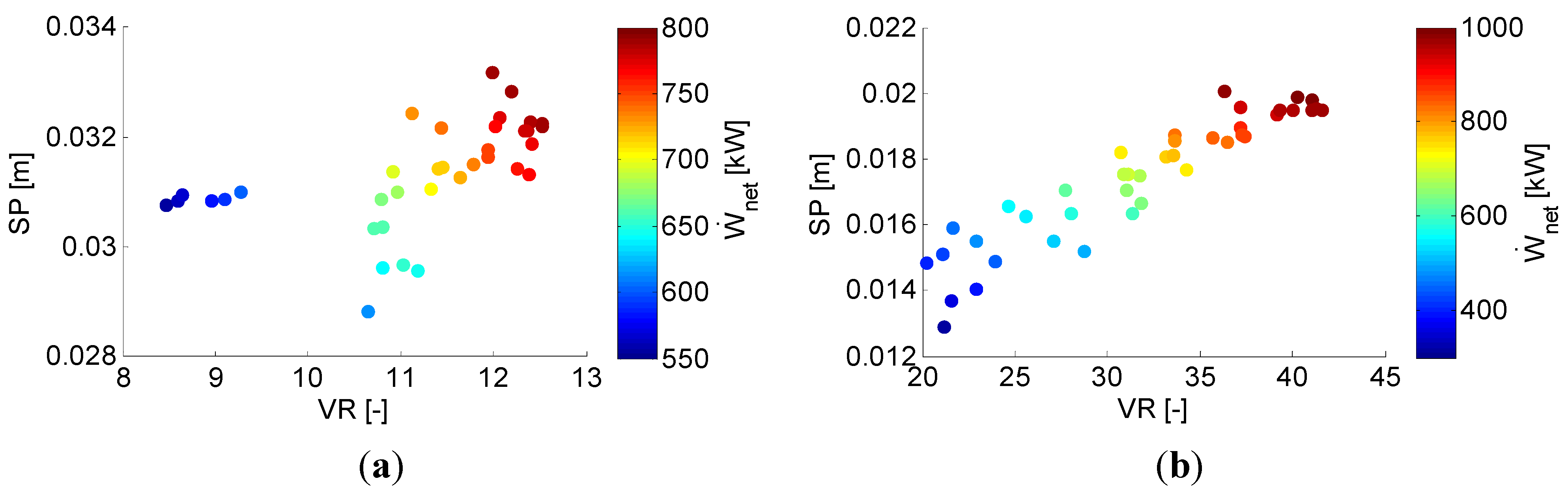
5.3. Turbine Performance Parameters

Both the SP and VR are plotted in Figure 13a,b for, respectively, the SCORC and TCORC. Considering the discussion in Section 3.4, the fixed isentropic efficiency of 0.7 is deemed realistic, while higher isentropic efficiencies are clearly attainable. For both cycle types, the VR is consistently lower than 50, with the TCORC exhibiting the largest VR. For increased VR, an increase in power output is noted. The size parameter becomes lower than 0.2 m for the TCORC. However, the SP has a lower influence on the isentropic efficiency then the VR. Furthermore, a conservative value of the isentropic efficiency was used.

Figure 13. Size parameter (SP) and volume ratio (VR) for (a) SCORC and (b) TCORC.

Figure 13. Size parameter (SP) and volume ratio (VR) for (a) SCORC and (b) TCORC.

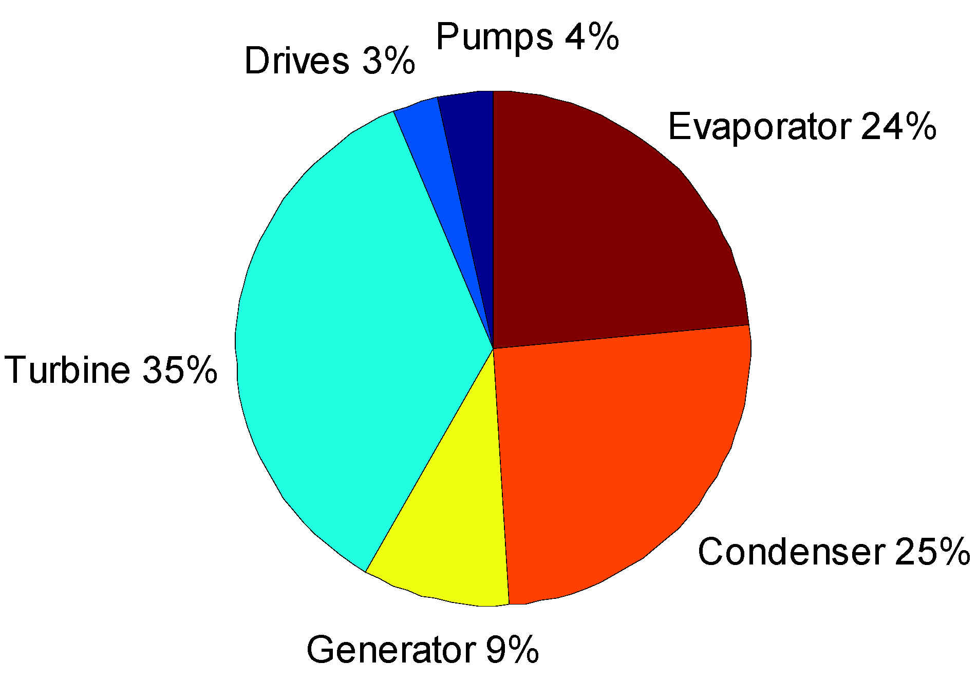
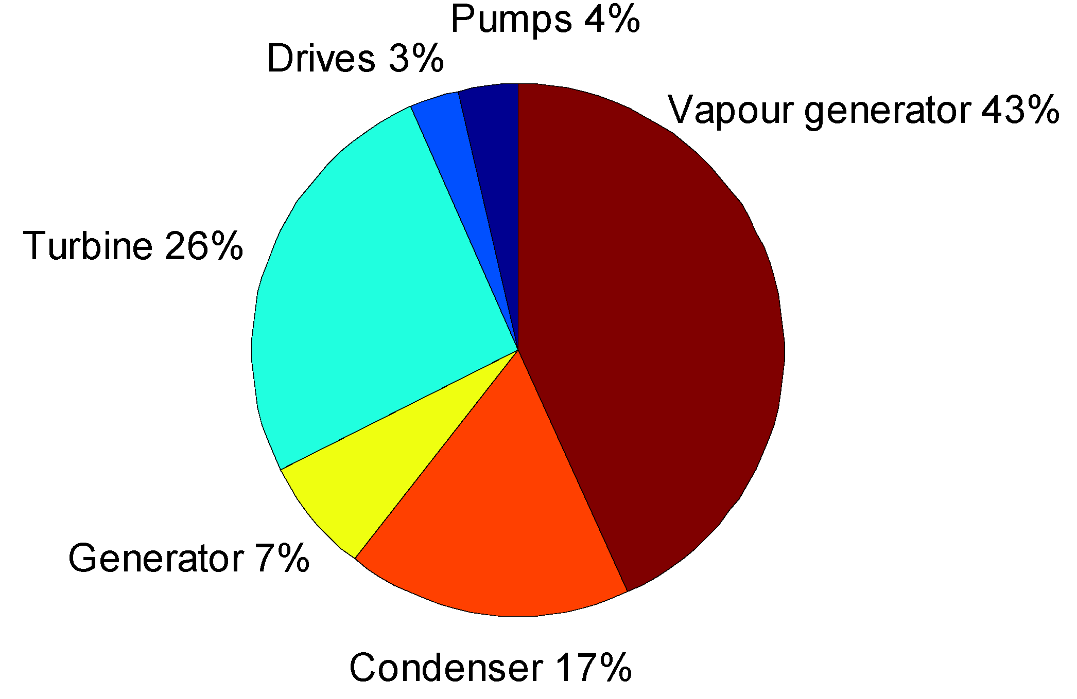
5.4. Distribution of the Costs

Identifying the distribution of the costs is a primary step in determining the focus for further optimization and development. Figure 14 shows the partition of the costs at minimum SIC for the SCORC while Figure 15 shows it for the TCORC. The distribution of the cost for the SCORC is in line with previous research done by the authors [32]. For the SCORC, the turbine amounts for the largest cost, followed by the condenser and evaporator. The sum of the generator, drives, and pumps results in the lowest share of costs.

Figure 14. Distribution of the cost at minimum SIC for the SCORC.

Figure 14. Distribution of the cost at minimum SIC for the SCORC.

Figure 15. Distribution of the cost at minimum SIC for the TCORC.

Figure 15. Distribution of the cost at minimum SIC for the TCORC.

In contrast, the vapor generator of the TCORC accounts for the largest cost, followed by the turbine and condenser. Thus, for the SCORC, it is reasonable to consider the turbine a key component for further development. While for TCORC, the vapor generator is the critical part, followed by the turbine.

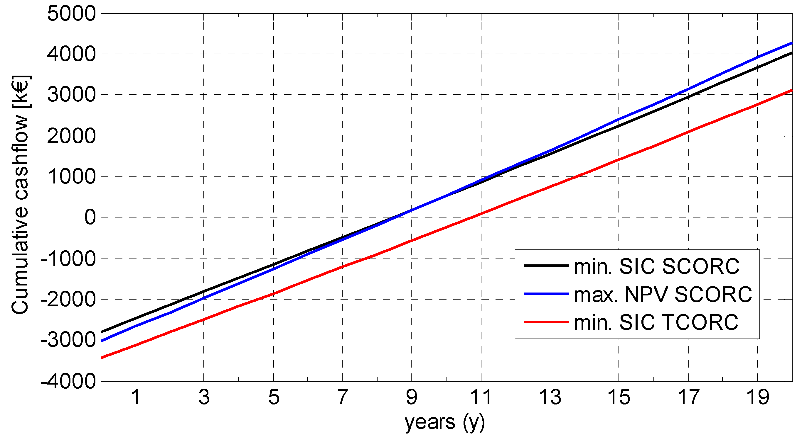
5.5. Financial Analysis and Decision Making

The Pareto fronts from Figure 3 and Figure 4 can be effectively used as input for the financial appraisal. As this is a post-processing step, no new design calculations are required. As such, several scenarios can be quickly evaluated. The calculation time is less than five seconds. These Pareto fronts could also be directly used as input for decision makers. The complexity of the design model is thus avoided in this phase.

A workshop [80] was organized between ORC manufacturers and end-users to verify the parameters of the NPV calculation listed in Table 11. The presented values are based on the market situation of Flanders, Belgium in 2013.

Table 11. Assumptions for net present value (NPV) calculation.

Parameter	Value
ORC lifetime (y)	20
discount rate (%)	6
production hours (h/y)	8000
price electricity (€/MWh)	69.6
increase electricity price (%/y)	0.50
maintenance cost ($C_{maintenance}/C_{TM}$)	0.02

Table 11. Assumptions for net present value (NPV) calculation.

Parameter	Value
ORC lifetime (y)	20
discount rate (%)	6
production hours (h/y)	8000
price electricity (€/MWh)	69.6
increase electricity price (%/y)	0.50
maintenance cost ($C_{maintenance}/C_{TM}$)	0.02

The results of the NPV calculation are given in Table 12 for both the point of minimum SIC and maximum NPV. All points show a positive NPV value, which means they would be cost-effective under the current assumptions. The simple payback period does not represent the best criterion for financial decision-making, but is often used in practice and shown here for completeness. For the presented case, the SCORC is flagged as the cycle of choice. The SCORC has an NPV that is 786 k€ higher than the NPV of the TCORC. Furthermore, the payback time is roughly two years less than for the TCORC.

Table 12. Results of the NPV calculation.

Case	${\dot{W}}_{net}$ (kW)	SIC (€/kWe)	NPV (k€)	Payback Time (y)
Min. SIC SCORC	681.8	4114	1070	8.46
Min. SIC TCORC	681.3	5044	284	10.70
Max. NPV SCORC	731.3	4138	1126	8.52
Max. NPV TCORC	681.3	5044	284	10.70

Table 12. Results of the NPV calculation.

Case	${\dot{W}}_{net}$ (kW)	SIC (€/kWe)	NPV (k€)	Payback Time (y)
Min. SIC SCORC	681.8	4114	1070	8.46
Min. SIC TCORC	681.3	5044	284	10.70
Max. NPV SCORC	731.3	4138	1126	8.52
Max. NPV TCORC	681.3	5044	284	10.70

Furthermore, the point of minimum SIC does not necessarily result in maximum NPV. For the SCORC, an ORC with a net power output 7.3% larger than ${\dot{W}}_{net,SIC}$, provides an increase of the NPV of 5.2%. This is directly related to the cash flow shown in Figure 16. A higher investment cost with an associated higher power output can lead in the long-term to higher profits. While a lower SIC, obviously, always leads to a lower payback time. For the TCORC, even in the long-term, a higher power output than ${\dot{W}}_{net,SIC}$ does not result in improved NPV, due to the very large increase in SIC (see Figure 4).

Figure 16. Cumulative cash flow for min. SIC SCORC, min. SIC TCORC and max. NPV SCORC.

Figure 16. Cumulative cash flow for min. SIC SCORC, min. SIC TCORC and max. NPV SCORC.

The presented results are only valid under the assumptions presented here and for this specific case. This analysis provides by no means a general conclusion about the profitability of the TCORC or SCORC. Using another working fluid, changing the type of waste heat carrier, or changing the cost structure could result in different conclusions. Also, installation of these systems in practice may induce different additional costs related to, i.e. installation, contractor’s fees, and contingencies. The aim of this work is therefore to introduce the optimization framework. In subsequent studies, other cases will be investigated, more working fluids will be considered and an added sensitivity analysis on the assumptions will be provided. As such, general conclusions about ORC architectures and their applicability can be formulated.

6. Conclusions

In this work a novel framework for designing optimized ORC systems is proposed based on a multi-objective optimization scheme in combination with financial appraisal in a post-processing step. This novel way of optimizing and interpreting results was applied on an incinerator waste heat recovery case. Both the SCORC and TCORC are investigated and compared using the suggested optimization strategy. The conclusions are summarized below:

The TCORC provides a 31.5% increase in net power output over the subcritical ORC, but with an increased SIC of 72.8%. When comparing both the SCORC and TCORC at minimum SIC, the net power output is almost equal. However, the SIC for the TCORC is increased by 22%.

The SIC for the SCORC is highly sensitive to variations in the pinch point temperature difference in contrast to the TCORC. Other significant parameters for the SCORC are the mass flux rates in the heat exchangers and the condensation temperature. While for the TCORC, the turbine inlet temperature and the condensation temperature are the factors with the highest sensitivity on the SIC.

For the SCORC, the turbine amounts to the highest cost (35%), while for the TCORC this is the vapor generator (43%). Therefore, stating the high importance of the vapor generator design.

In the financial appraisal, the SCORC clearly outperforms the TCORC. Furthermore, while the minimum SIC leads to the lowest payback time this does not necessarily lead to the highest NPV. For the SCORC, an ORC with a net power output 7.3% larger than the net power output at minimum SIC, provides an increased NPV of 5.2%.

The given results are only valid for the case and assumptions presented in this study. They do not count as general recommendations for cycle architectures as the aim of this work is to introduce the optimization framework. In order to provide general recommendations, further work will include additional cases, more working fluids, different heat carrier types and a sensitivity analyses on each of the assumptions made.

References

1. Bronicki, L. Short review of the long history of ORC power systems. In Proceedings of the ORC2013, Rotterdam, The Netherlands, 7–8 October 2013.
2. Tchanche, B.F.; Pétrissans, M.; Papadakis, G. Heat resources and organic Rankine cycle machines. Renew. Sustain. Energy Rev. 2014, 39, 1185–1199. [Google Scholar]
3. Quoilin, S.; Broek, M.V.D.; Declaye, S.; Dewallef, P.; Lemort, V. Techno-economic survey of Organic Rankine Cycle (ORC) systems. Renew. Sustain. Energy Rev. 2013, 22, 168–186. [Google Scholar] [CrossRef]
4. Tchanche, B.F.; Lambrinos, G.; Frangoudakis, A.; Papadakis, G. Low-grade heat conversion into power using organic Rankine cycles–A review of various applications. Renew. Sustain. Energy Rev. 2011, 15, 3963–3979. [Google Scholar] [CrossRef]
5. Lai, N.A.; Fischer, J. Efficiencies of power flash cycles. Energy 2012, 44, 1017–1027. [Google Scholar] [CrossRef]
6. Fischer, J. Comparison of trilateral cycles and organic Rankine cycles. Energy 2011, 36, 6208–6219. [Google Scholar] [CrossRef]
7. Smith, I.K. Development of the trilateral flash cycle system Part1: Fundamental considerations. Proc. Inst. Mech. Eng. Part A J. Power Energy 1993, 207, 179–194. [Google Scholar] [CrossRef]
8. Heberle, F.; Preißinger, M.; Brüggemann, D. Zeotropic mixtures as working fluids in Organic Rankine Cycles for low-enthalpy geothermal resources. Renew. Energy 2012, 37, 364–370. [Google Scholar] [CrossRef]
9. Lecompte, S.; Ameel, B.; Ziviani, D.; van den Broek, M.; de Paepe, M. Exergy analysis of zeotropic mixtures as working fluids in Organic Rankine Cycles. Energy Convers. Manag. 2014, 85, 727–739. [Google Scholar] [CrossRef]
10. Chys, M.; van den Broek, M.; Vanslambrouck, B.; Paepe, M.D. Potential of zeotropic mixtures as working fluids in organic Rankine cycles. Energy 2012, 44, 623–632. [Google Scholar] [CrossRef]
11. Stijepovic, M.Z.; Papadopoulos, A.I.; Linke, P.; Grujic, A.S.; Seferlis, P. An exergy composite curves approach for the design of optimum multi-pressure organic Rankine cycle processes. Energy 2014, 69, 285–298. [Google Scholar] [CrossRef]
12. Gnutek, Z.; Bryszewska-Mazurek, A. The thermodynamic analysis of multicycle ORC engine. Energy 2001, 26, 1075–1082. [Google Scholar] [CrossRef]
13. Angelino, G.; Colonna, P. Multicomponent working fluids for organic Rankine cycles (ORCs). Energy 1998, 23, 449–463. [Google Scholar] [CrossRef]
14. Saleh, B.; Koglbauer, G.; Wendland, M.; Fischer, J. Working fluids for low-temperature organic Rankine cycles. Energy 2007, 32, 1210–1221. [Google Scholar] [CrossRef]
15. Schuster, A.; Karellas, S.; Aumann, R. Efficiency optimization potential in supercritical Organic Rankine Cycles. Energy 2010, 35, 1033–1039. [Google Scholar] [CrossRef]
16. Karellas, S.; Schuster, A.; Leontaritis, A.-D. Influence of supercritical ORC parameters on plate heat exchanger design. Appl. Therm. Eng. 2012, 33–34, 70–76. [Google Scholar]
17. Wang, Z.Q.; Zhou, N.J.; Guo, J.; Wang, X.Y. Fluid selection and parametric optimization of organic Rankine cycle using low temperature waste heat. Energy 2012, 40, 107–115. [Google Scholar] [CrossRef]
18. Yamada, N.; Mohamad, M.N.A.; Kien, T.T. Study on thermal efficiency of low- to medium-temperature organic Rankine cycles using HFO−1234yf. Renew. Energy 2012, 41, 368–375. [Google Scholar] [CrossRef]
19. Liu, B.-T.; Chien, K.-H.; Wang, C.-C. Effect of working fluids on organic Rankine cycle for waste heat recovery. Energy 2004, 29, 1207–1217. [Google Scholar] [CrossRef]
20. Dai, Y.; Wang, J.; Gao, L. Parametric optimization and comparative study of organic Rankine cycle (ORC) for low grade waste heat recovery. Energy Convers. Manag. 2009, 50, 576–582. [Google Scholar] [CrossRef]
21. Hung, T.C.; Wang, S.K.; Kuo, C.H.; Pei, B.S.; Tsai, K.F. A study of organic working fluids on system efficiency of an ORC using low-grade energy sources. Energy 2010, 35, 1403–1411. [Google Scholar] [CrossRef]
22. Chen, H.; Goswami, D.Y.; Stefanakos, E.K. A review of thermodynamic cycles and working fluids for the conversion of low-grade heat. Renew. Sustain. Energy Rev. 2010, 14, 3059–3067. [Google Scholar] [CrossRef]
23. Ho, T.; Mao, S.S.; Greif, R. Comparison of the Organic Flash Cycle (OFC) to other advanced vapor cycles for intermediate and high temperature waste heat reclamation and solar thermal energy. Energy 2012, 42, 213–223. [Google Scholar] [CrossRef]
24. Öhman, H.; Lundqvist, P. Comparison and analysis of performance using Low Temperature Power Cycles. Appl. Therm. Eng. 2013, 52, 160–169. [Google Scholar] [CrossRef]
25. Brigham, E.F.; Ehrhardt, M.C. Financial Management: Theory and Practice, 14th ed.; South-Western Cengage Learning: Mason, USA, 2014. [Google Scholar]
26. Madhawa Hettiarachchi, H.D.; Golubovic, M.; Worek, W.M.; Ikegami, Y. Optimum design criteria for an Organic Rankine cycle using low-temperature geothermal heat sources. Energy 2007, 32, 1698–1706. [Google Scholar]
27. Cayer, E.; Galanis, N.; Nesreddine, H. Parametric study and optimization of a transcritical power cycle using a low temperature source. Appl. Energy 2010, 87, 1349–1357. [Google Scholar] [CrossRef]
28. Zhang, S.; Wang, H.; Guo, T. Performance comparison and parametric optimization of subcritical Organic Rankine Cycle (ORC) and transcritical power cycle system for low-temperature geothermal power generation. Appl. Energy 2011, 88, 2740–2754. [Google Scholar] [CrossRef]
29. Quoilin, S.; Declaye, S.; Tchanche, B.F.; Lemort, V. Thermo-economic optimization of waste heat recovery Organic Rankine Cycles. Appl. Therm. Eng. 2011, 31, 2885–2893. [Google Scholar] [CrossRef]
30. Wang, J.; Yan, Z.; Wang, M.; Ma, S.; Dai, Y. Thermodynamic analysis and optimization of an (organic Rankine cycle) ORC using low grade heat source. Energy 2013, 49, 356–365. [Google Scholar] [CrossRef]
31. Wang, J.; Yan, Z.; Wang, M.; Li, M.; Dai, Y. Multi-objective optimization of an organic Rankine cycle (ORC) for low grade waste heat recovery using evolutionary algorithm. Energy Convers. Manag. 2013, 71, 146–158. [Google Scholar] [CrossRef]
32. Lecompte, S.; Huisseune, H.; van den Broek, M.; de Schampheleire, S.; de Paepe, M. Part load based thermo-economic optimization of the Organic Rankine Cycle (ORC) applied to a combined heat and power (CHP) system. Appl. Energy 2013, 111, 871–881. [Google Scholar] [CrossRef]
33. Pierobon, L.; Nguyen, T.-V.; Larsen, U.; Haglind, F.; Elmegaard, B. Multi-objective optimization of organic Rankine cycles for waste heat recovery: Application in an offshore platform. Energy 2013, 58, 538–549. [Google Scholar] [CrossRef]
34. Astolfi, M.; Romano, M.C.; Bombarda, P.; Macchi, E. Binary ORC (Organic Rankine Cycles) power plants for the exploitation of medium–low temperature geothermal sources–Part B: Techno-economic optimization. Energy 2014, 66, 435–446. [Google Scholar]
35. Shu, G.; Yu, G.; Tian, H.; Wei, H.; Liang, X. A Multi-Approach Evaluation System (MA-ES) of Organic Rankine Cycles (ORC) used in waste heat utilization. Appl. Energy 2014, 132, 325–338. [Google Scholar] [CrossRef]
36. Li, Y.-R.; Du, M.-T.; Wu, C.-M.; Wu, S.-Y.; Liu, C. Potential of organic Rankine cycle using zeotropic mixtures as working fluids for waste heat recovery. Energy 2014, 77, 509–519. [Google Scholar] [CrossRef]
37. Li, Y.-R.; Du, M.-T.; Wu, C.-M.; Wu, S.-Y.; Liu, C.; Xu, J.-L. Economical evaluation and optimization of subcritical organic Rankine cycle based on temperature matching analysis. Energy 2014, 68, 238–247. [Google Scholar] [CrossRef]
38. Imran, M.; Park, B.S.; Kim, H.J.; Lee, D.H.; Usman, M.; Heo, M. Thermo-economic optimization of Regenerative Organic Rankine Cycle for waste heat recovery applications. Energy Convers. Manag. 2014, 87, 107–118. [Google Scholar] [CrossRef]
39. Nusiaputra, Y.Y.; Wiemer, H.-J.; Kuhn, D. Thermal-Economic modularization of small, organic Rankine cycle power plants for mid-enthalpy geothermal fields. Energies 2014, 7, 4221–4240. [Google Scholar] [CrossRef]
40. Li, M.; Wang, J.; Li, S.; Wang, X.; He, W.; Dai, Y. Thermo-economic analysis and comparison of a CO2 transcritical power cycle and an organic Rankine cycle. Geothermics 2014, 50, 101–111. [Google Scholar] [CrossRef]
41. Toffolo, A.; Lazzaretto, A.; Manente, G.; Paci, M. A multi-criteria approach for the optimal selection of working fluid and design parameters in Organic Rankine Cycle systems. Appl. Energy 2014, 121, 219–232. [Google Scholar] [CrossRef]
42. Meinel, D.; Wieland, C.; Spliethoff, H. Economic comparison of ORC (Organic Rankine cycle) processes at different scales. Energy 2014, 74, 694–706. [Google Scholar] [CrossRef]
43. Deb, K. Multi-Objective Optimization Using Evolutionary Algorithms; Wiley: Chicester, West Sussex, UK, 2001. [Google Scholar]
44. Mago, P.J.; Chamra, L.M.; Srinivasan, K.; Somayaji, C. An examination of regenerative organic Rankine cycles using dry fluids. Appl. Therm. Eng. 2008, 28, 998–1007. [Google Scholar] [CrossRef]
45. Hung, T.C.; Shai, T.Y.; Wang, S.K. A review of organic rankine cycles (ORCs) for the recovery of low-grade waste heat. Energy 1997, 22, 661–667. [Google Scholar] [CrossRef]
46. Lai, N.A.; Wendland, M.; Fischer, J. Working fluids for high-temperature organic Rankine cycles. Energy 2011, 36, 199–211. [Google Scholar] [CrossRef]
47. Martin, H. Economic optimization of compact heat exchangers. In Proceedings of the EF-Conference on Compact Heat Exchangers and Enhancement Technology for the Process Industries, Banff, AB, Canada, 18–23 July 1999.
48. Han, D.-H.; Lee, K.-J.; Kim, Y.-H. Experiments on the characteristics of evaporation of R410A in brazed plate heat exchangers with different geometric configurations. Appl. Therm. Eng. 2003, 23, 1209–1225. [Google Scholar] [CrossRef]
49. Han, D.; Lee, K.; Kim, Y. The characteristics of condensation in brazed plate heat and exchangers with different chevron angles. J. Korean Phys. Soc. 2003, 43, 66–73. [Google Scholar]
50. Hsieh, Y.Y.; Lin, T.F. Evaporation heat transfer and pressure drop of refrigerant R-410A flow in a vertical plate heat exchanger. J. Heat Transf. 2003, 125, 852–857. [Google Scholar] [CrossRef]
51. Yan, Y.Y.; Lin, T.F. Evaporation heat transfer and pressure drop of refrigerant R-134a in a plate heat exchanger. J. Heat Transf. 1999, 121, 118–127. [Google Scholar] [CrossRef]
52. Kuo, C.-R.; Hsu, S.-W.; Chang, K.-H.; Wang, C.-C. Analysis of a 50kW organic Rankine cycle system. Energy 2011, 36, 5877–5885. [Google Scholar] [CrossRef]
53. Walraven, D.; Laenen, B.; D’haeseleer, W. Comparison of shell-and-tube with plate heat exchangers for the use in low-temperature organic Rankine cycles. Energy Convers. Manag. 2014, 87, 227–237. [Google Scholar] [CrossRef]
54. García-Cascales, J.R.; Vera-García, F.; Corberán-Salvador, J.M.; Gonzálvez-Maciá, J. Assessment of boiling and condensation heat transfer correlations in the modelling of plate heat exchangers. Int. J. Refrig. 2007, 30, 1029–1041. [Google Scholar] [CrossRef]
55. Petukhov, B.S.; Krasnoschekov, E.A.; Protopopov, V.S. An investigation of heat transfer to fluid flowing in pipes under supercritical conditions. In Proceedings of the International Developments in Heat Transfer, University of Colorado, Boulder, CO, USA, 8–12 January 1961; Volume 67, pp. 569–578.
56. Wang, L.; Sundén, B.; Manglik, R.M. Plate Heat Exchangers: Design, Applications and Performance; WIT Press: Southampton, UK, 2007. [Google Scholar]
57. Barbazza, L.; Pierobon, L.; Mirandola, A.; Haglind, F. Optimal design of compact organic Rankine cycle units for domestic solar applications. Therm. Sci. 2014, 18, 811–822. [Google Scholar] [CrossRef] [Green Version]
58. Wang, L.; Sundén, B. Optimal design of plate heat exchangers with and without pressure drop specifications. Appl. Therm. Eng. 2003, 23, 295–311. [Google Scholar] [CrossRef]
59. Turton, R.; Bailie, R.C.; Whiting, W.B.; Shaeiwitz, J.; Bhattacharyya, D. Analysis, Synthesis and Design of Chemical Processes, 4th ed.; Pearson Education: Ann Arbor, MI, USA, 2013. [Google Scholar]
60. Lee, Y.-R.; Kuo, C.-R.; Wang, C.-C. Transient response of a 50 kW organic Rankine cycle system. Energy 2012, 48, 532–538. [Google Scholar] [CrossRef]
61. Declaye, S.; Quoilin, S.; Guillaume, L.; Lemort, V. Experimental study on an open-drive scroll expander integrated into an ORC (Organic Rankine Cycle) system with R245fa as working fluid. Energy 2013, 55, 173–183. [Google Scholar] [CrossRef]
62. Sauret, E.; Rowlands, A.S. Candidate radial-inflow turbines and high-density working fluids for geothermal power systems. Energy 2011, 36, 4460–4467. [Google Scholar] [CrossRef]
63. Kang, S.H. Design and experimental study of ORC (organic Rankine cycle) and radial turbine using R245fa working fluid. Energy 2012, 41, 514–524. [Google Scholar] [CrossRef]
64. Luján, J.M.; Serrano, J.R.; Dolz, V.; Sánchez, J. Model of the expansion process for R245fa in an Organic Rankine Cycle (ORC). Appl. Therm. Eng. 2012, 40, 248–257. [Google Scholar] [CrossRef]
65. Da Lio, L.; Manente, G.; Lazzaretto, A. New efficiency charts for the optimum design of axial flow turbines for organic Rankine cycles. Energy 2014, 77, 447–459. [Google Scholar] [CrossRef]
66. Klein, S.A. Engineering Equation Solver; F-Chart Software: Middleton, WI, USA, 2010. [Google Scholar]
67. Lemmon, E.W.; Span, R. Short fundamental equations of state for 20 industrial fluids. J. Chem. Eng. Data 2006, 51, 785–850. [Google Scholar] [CrossRef]
68. Lemmon, E.W.; Huber, M.L.; McLinden, M.O. Reference Fluid Thermodynamic and Transport Properties-REFPROP, Version 9.1; National Institute of Standards and Technology: Gaithersburg, MD, USA, 2013.
69. Huber, M.L.; Laesecke, A.; Perkins, R.A. Model for the viscosity and thermal conductivity of refrigerants, including a new correlation for the viscosity of R134a. Ind. Eng. Chem. Res. 2003, 42, 3163–3178. [Google Scholar] [CrossRef]
70. Marsh, K.N.; Perkins, R.A.; Ramires, M.L.V. Measurement and correlation of the thermal conductivity of propane from 86 to 600 K at pressures to 70 MPa. J. Chem. Eng. Data 2002, 47, 932–940. [Google Scholar] [CrossRef]
71. Macchi, E. The choice of working fluid: The most important step for a successful organic Rankine cycle (and an efficient turbine), Keynote lecture. In Proceedings of the ASME ORC2013, Rotterdam, The Netherlands, 7–8 October 2013.
72. Maraver, D.; Royo, J.; Lemort, V.; Quoilin, S. Systematic optimization of subcritical and transcritical organic Rankine cycles (ORCs) constrained by technical parameters in multiple applications. Appl. Energy 2014, 117, 11–29. [Google Scholar] [CrossRef]
73. Shah, R.K.; Subbarao, E.C.; Mashelkar, R.A. Heat Transfer Equipment Design; CRC Press: New York, NY, USA, 1988. [Google Scholar]
74. Deb, K.; Pratap, A.; Agarwal, S.; Meyarivan, T. A fast and elitist multiobjective genetic algoritm: NSGA-II. IEEE Trans. Evol. Comput. 2002, 6, 182–197. [Google Scholar] [CrossRef]
75. Feng, Y.; Zhang, Y.; Li, B.; Yang, J.; Shi, Y. Sensitivity analysis and thermoeconomic comparison of ORCs (organic Rankine cycles) for low temperature waste heat recovery. Energy 2015, 82, 664–677. [Google Scholar] [CrossRef]
76. Ahmadi, P.; Dincer, I.; Rosen, M.A. Thermodynamic modeling and multi-objective evolutionary-based optimization of a new multigeneration energy system. Energy Convers. Manag. 2013, 76, 282–300. [Google Scholar] [CrossRef]
77. Ahmadi, P.; Dincer, I.; Rosen, M.A. Thermoeconomic multi-objective optimization of a novel biomass-based integrated energy system. Energy 2014, 68, 958–970. [Google Scholar] [CrossRef]
78. Hajabdollahi, Z.; Hajabdollahi, F.; Tehrani, M.; Hajabdollahi, H. Thermo-economic environmental optimization of Organic Rankine Cycle for diesel waste heat recovery. Energy 2013, 63, 142–151. [Google Scholar] [CrossRef]
79. MATLAB Release 2013b, The MathWorks, Inc.: Natick, MA, USA.
80. Lemmens, S.; Lecompte, S.; de Paepe, M. Workshop Financial Appraisal of ORC Systems. In Presented at ORCNext Project, Antwerp, Belgium, 18 September 2014.