Review of Power Conversion and Conditioning Systems for Stationary Electrochemical Storage

Abstract

This paper deals with the power conversion system architectures to interface a stationary electrochemical storage installation with the network. Theoretical justifications about the conversion system layouts and control, used for actual Italian installations, are given. This paper aims at giving the power energy society an overview of actual possibilities of static conversion of d.c. battery sources.

1. Introduction

An electrochemical energy stationary storage system (EESSS), as a matter of principle, could be directly connected to the HV network by means of an inverter. Nevertheless, this approach of “direct connection” is not efficient and the chief reason must be attributed to the fact that the EESSS voltage, during the discharge stage, is not constant. For instance, the sodium sulphide (NaS) battery [1,2,3,4,5,6] voltage ranges, during discharge, between 100% and 64%, the lithium-ion battery one ranges between 100% and 70%. This behaviour implies two consequences:

➢

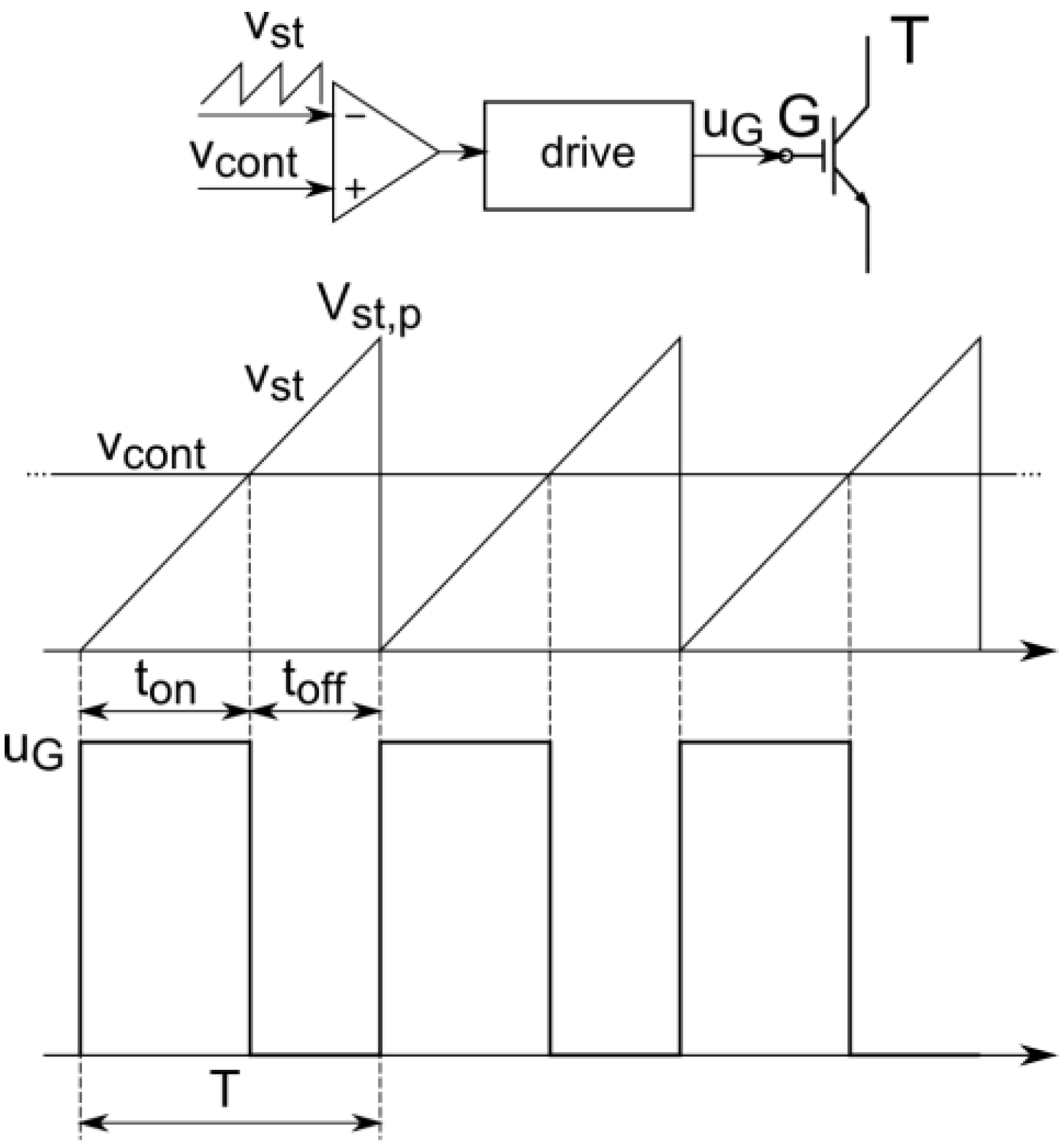
With a direct inverter−EESSS connection, the EESSS (e.g., a battery) voltage variations would imply a remarkable increase of the harmonic content (h) in the inverter output voltage. This effect is due to the fact that an inverter generally operates according to a PWM switching scheme [7,8] (see Section 3) in which, in order to pilot the inverter switches, a sinusoidal reference signal is compared with a sawtooth signal with higher frequency. The ratio between the reference signal frequency and the sawtooth one is defined by means of m_f [8]. The EESSS voltage fluctuations imply the variations of the inverter modulation index (m_a) [8], which is the ratio between the reference signal amplitude and the sawtooth one. Consequently, as shown in Table 1, the harmonic content (h) of the inverter voltage increases, so penalizing the inverter output quality.

➢

A Δu_% percentage EESSS voltage variation with respect to the rated value requires the inverter component overrating of 1 + Δu_% as for both the voltage and the current (maximum current corresponding to minimum battery voltage), resulting in an inverter power oversizing of about 1 + 2Δu_%. By hypothesizing a current and voltage variation of 20%, the inverter rated power can be inferred by the following simple relation:

P = ΔV_max·ΔI_max = V_n(1 + 20%)·I_n(1 + 20%) ≈ 1.40P_n = P_n + ΔP

Hence, it is preferable to connect an EESSS to the electrical network by means of a two-stage converter [9,10,11] (see Figure 1). It consists of a first stage made by a d.c.-d.c. converter and of a second stage made by a d.c.-a.c. converter so enabling to keep the inverter d.c. side voltage U_o constant.

Table 1. Harmonic content h as a function of the amplitude modulation m_a and of the frequency modulation m_f indexes (greyed rows are absent in three-phase inverters provided m_f is a multiple of three).

	ma =	0.100	0.200	0.300	0.400	0.500	0.600	0.700	0.800	0.900	1.000
h=
mf		1.265	1.242	1.204	1.151	1.084	1.006	0.917	0.818	0.712	0.601
mf ± 2		0.004	0.016	0.035	0.061	0.093	0.131	0.174	0.220	0.268	0.318
mf ± 4		−	−	−	0.001	0.001	0.003	0.005	0.008	0.012	0.018
2mf ± 1		0.099	0.190	0.268	0.326	0.361	0.370	0.354	0.314	0.255	0.181
2mf ± 3		−	0.003	0.011	0.024	0.044	0.071	0.103	0.139	0.177	0.212
2mf ± 5		−	−	−	−	0.001	0.003	0.007	0.013	0.021	0.033
3mf		0.401	0.335	0.237	0.123	0.011	0.083	0.146	0.171	0.157	0.113
3mf ± 2		0.012	0.044	0.089	0.139	0.180	0.203	0.203	0.176	0.127	0.062
3mf ± 4		−	0.001	0.004	0.012	0.026	0.047	0.074	0.105	0.134	0.158
4mf − 5		−	−	0.002	0.006	0.017	0.034	0.058	0.084	0.107	0.119
4mf − 3		0.002	0.012	0.035	0.070	0.106	0.132	0.137	0.115	0.068	0.009
4mf ± 1		0.095	0.163	0.185	0.157	0.091	0.008	0.064	0.105	0.105	0.068
4mf + 3		0.002	0.012	0.035	0.070	0.106	0.132	0.137	0.114	0.068	0.007
4mf + 5		−	−	0.002	0.006	0.017	0.034	0.057	0.082	0.101	0.105
5mf − 4		−	0.004	0.015	0.039	0.069	0.094	0.101	0.080	0.035	0.019
5mf − 2		0.019	0.064	0.108	0.124	0.097	0.037	0.030	0.073	0.075	0.038
5mf		0.217	0.120	0.006	0.077	0.102	0.068	0.002	0.056	0.076	0.052
5mf + 2		0.019	0.064	0.108	0.124	0.097	0.037	0.030	0.073	0.074	0.035
5mf + 4		−	0.004	0.015	0.039	0.069	0.095	0.102	0.084	0.044	−
6mf − 5		−	0.001	0.007	0.023	0.047	0.072	0.080	0.061	0.022	0.018
6mf − 3		0.004	0.024	0.059	0.088	0.086	0.046	0.013	0.056	0.055	0.016
6mf − 1		0.089	0.123	0.085	0.005	0.060	0.070	0.027	0.031	0.058	0.039
6mf + 1		0.089	0.123	0.085	0.005	0.060	0.070	0.027	0.030	0.056	0.032
6mf + 3		0.004	0.024	0.059	0.088	0.086	0.045	0.015	0.060	0.067	0.040
6mf + 5		−	0.001	0.007	0.023	0.047	0.069	0.070	0.039	0.021	0.082

Table 1. Harmonic content h as a function of the amplitude modulation m_a and of the frequency modulation m_f indexes (greyed rows are absent in three-phase inverters provided m_f is a multiple of three).

	ma =	0.100	0.200	0.300	0.400	0.500	0.600	0.700	0.800	0.900	1.000
h=
mf		1.265	1.242	1.204	1.151	1.084	1.006	0.917	0.818	0.712	0.601
mf ± 2		0.004	0.016	0.035	0.061	0.093	0.131	0.174	0.220	0.268	0.318
mf ± 4		−	−	−	0.001	0.001	0.003	0.005	0.008	0.012	0.018
2mf ± 1		0.099	0.190	0.268	0.326	0.361	0.370	0.354	0.314	0.255	0.181
2mf ± 3		−	0.003	0.011	0.024	0.044	0.071	0.103	0.139	0.177	0.212
2mf ± 5		−	−	−	−	0.001	0.003	0.007	0.013	0.021	0.033
3mf		0.401	0.335	0.237	0.123	0.011	0.083	0.146	0.171	0.157	0.113
3mf ± 2		0.012	0.044	0.089	0.139	0.180	0.203	0.203	0.176	0.127	0.062
3mf ± 4		−	0.001	0.004	0.012	0.026	0.047	0.074	0.105	0.134	0.158
4mf − 5		−	−	0.002	0.006	0.017	0.034	0.058	0.084	0.107	0.119
4mf − 3		0.002	0.012	0.035	0.070	0.106	0.132	0.137	0.115	0.068	0.009
4mf ± 1		0.095	0.163	0.185	0.157	0.091	0.008	0.064	0.105	0.105	0.068
4mf + 3		0.002	0.012	0.035	0.070	0.106	0.132	0.137	0.114	0.068	0.007
4mf + 5		−	−	0.002	0.006	0.017	0.034	0.057	0.082	0.101	0.105
5mf − 4		−	0.004	0.015	0.039	0.069	0.094	0.101	0.080	0.035	0.019
5mf − 2		0.019	0.064	0.108	0.124	0.097	0.037	0.030	0.073	0.075	0.038
5mf		0.217	0.120	0.006	0.077	0.102	0.068	0.002	0.056	0.076	0.052
5mf + 2		0.019	0.064	0.108	0.124	0.097	0.037	0.030	0.073	0.074	0.035
5mf + 4		−	0.004	0.015	0.039	0.069	0.095	0.102	0.084	0.044	−
6mf − 5		−	0.001	0.007	0.023	0.047	0.072	0.080	0.061	0.022	0.018
6mf − 3		0.004	0.024	0.059	0.088	0.086	0.046	0.013	0.056	0.055	0.016
6mf − 1		0.089	0.123	0.085	0.005	0.060	0.070	0.027	0.031	0.058	0.039
6mf + 1		0.089	0.123	0.085	0.005	0.060	0.070	0.027	0.030	0.056	0.032
6mf + 3		0.004	0.024	0.059	0.088	0.086	0.045	0.015	0.060	0.067	0.040
6mf + 5		−	0.001	0.007	0.023	0.047	0.069	0.070	0.039	0.021	0.082

Figure 1. Basic two-stage converter configuration.

Figure 1. Basic two-stage converter configuration.

2. Two-Stage Converter Architecture for EESSS

A two-stage converter basically consists in two coupled converters: the first one is a two-quadrant current reversible chopper, carrying out a d.c.-d.c. conversion and consisting of the combination of a step-down (buck) and of a step-up (boost) converter, the second one is a switch-mode d.c.-a.c inverter. Two possible d.c.-d.c. converter layouts are considered, namely layout 1 and layout 2 of Figure 2. In the following, their behaviour is analysed in EESSS charge and discharge operation in order to identify the more profitable configuration for stationary storage applications.

Figure 2. Main layouts of the d.c.-d.c. stage of the two-stage converter.

Figure 2. Main layouts of the d.c.-d.c. stage of the two-stage converter.

2.1. EESSS Discharge: Layout 1 vs. Layout 2 Behaviour

Let us suppose that an EESSS in discharge mode is connected to a layout 1 d.c.-d.c. converter and that the inductor current i_L is constantly not null. In this case the d.c.-d.c. converter operates as a step-up (boost) converter and T₁ conduction is permanently inhibited.

The converter output voltage U_o can then be expressed [12] as a function of the EESSS voltage U_b and of the duty cycle D of the d.c.-d.c. converter (i.e., of T₂ switch) as:

$$U_o=1/\left(1-D\right)\cdot U_b$$

(1)

Being 0 ≤ D ≤ 1, U_o is always greater than U_b. This condition enables electric power to flow from the battery to the network. As it is shown in Figure 3b, the battery current i_b is unidirectional and equal to i_L.

Figure 3. Layout 1 discharge operation: current and voltage waveforms (continuous conduction).

Figure 3. Layout 1 discharge operation: current and voltage waveforms (continuous conduction).

If an EESSS is connected, in the same condition above mentioned, to a layout 2 d.c.-d.c. converter (now operating as step-down − buck − converter, being T₂ inhibited), the output voltage U_o still depends upon the T₁ duty cycle D, and it is given by:

$$U_o=D\cdot U_b$$

(2)

since D ranges between 0 and 1, U_o is always lower than U_b. This condition allows the flow of power from the battery to the network but, in this case, the battery current i_b is not equal to i_L and it has an impulsive behaviour as it is shown in Figure 4.

2.2. EESSS Charge: Layout 1 vs. Layout 2

Let us suppose that an EESSS in charge condition is connected to a layout 1 d.c.-d.c. converter, and that the inductor current i_L is constantly not null. In this condition, the d.c.-d.c. converter operates as a step-down stage (T₂ is inhibited) and its output voltage (i.e., battery voltage U_b) still depends only upon the T₁ duty cycle D, and it is given by:

$$U_b=D\cdot U_o$$

(3)

Consequently, the battery voltage U_b is always lower than the input voltage U_o. In the EESSS charge mode this voltage behaviour has a key-role because the power flow from the grid to the battery is always guaranteed, so that the charge operation is possible directly from the grid. The battery current is unidirectional and non-impulsive (see Figure 5).

Figure 4. Layout 2 discharge operation: current and voltage waveforms (continuous conduction).

Figure 4. Layout 2 discharge operation: current and voltage waveforms (continuous conduction).

Figure 5. Layout 1 charge operation: current and voltage waveforms (continuous conduction).

Figure 5. Layout 1 charge operation: current and voltage waveforms (continuous conduction).

In the same charge above mentioned condition, a layout 2 converter, operates as a step-up converter (T₁ is inhibited) and the output voltage U_b is given by (D: T₂ duty cycle):

$$U_b=U_o/\left(1-D\right)$$

(4)

Therefore the battery voltage U_b is greater than U_o, as in the discharge operation; being U_o generally imposed by grid interface requirements, U_b maximum value could result in demanding specifications for EESSS and connected electrical installation. Moreover, the current is again pulsed, as it is shown in Figure 6. Hence, Layout 1 configuration is preferable in both charge and discharge operation.

Figure 6. Layout 2 charge operation: current and voltage waveforms (continuous conduction).

Figure 6. Layout 2 charge operation: current and voltage waveforms (continuous conduction).

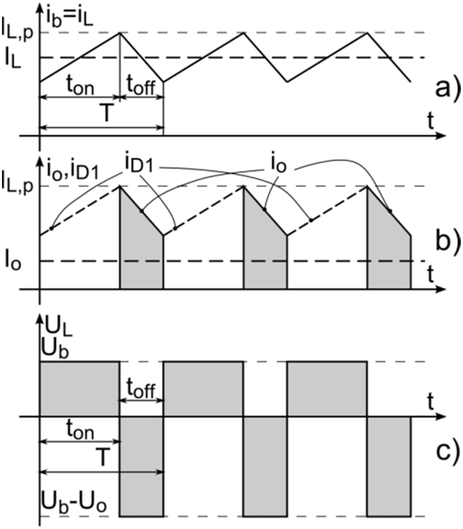
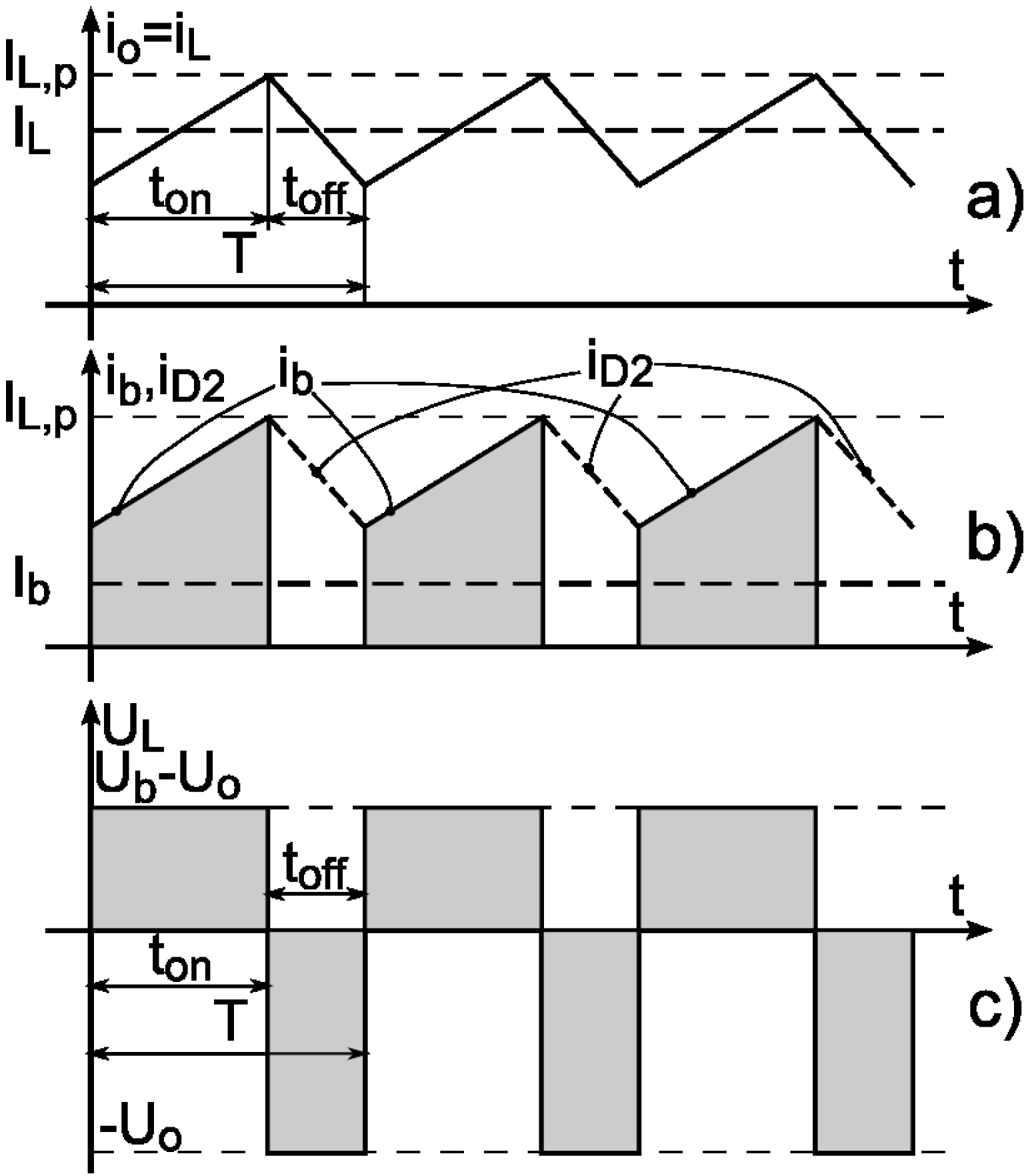
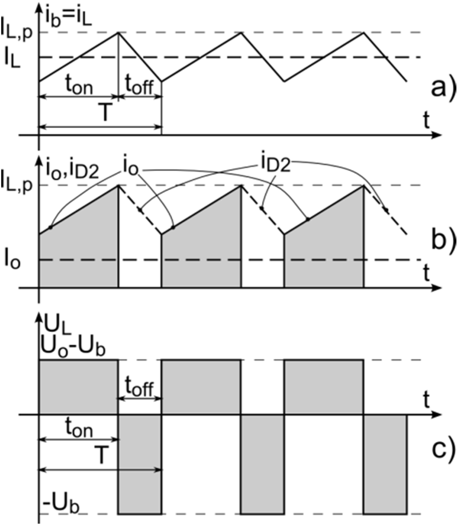
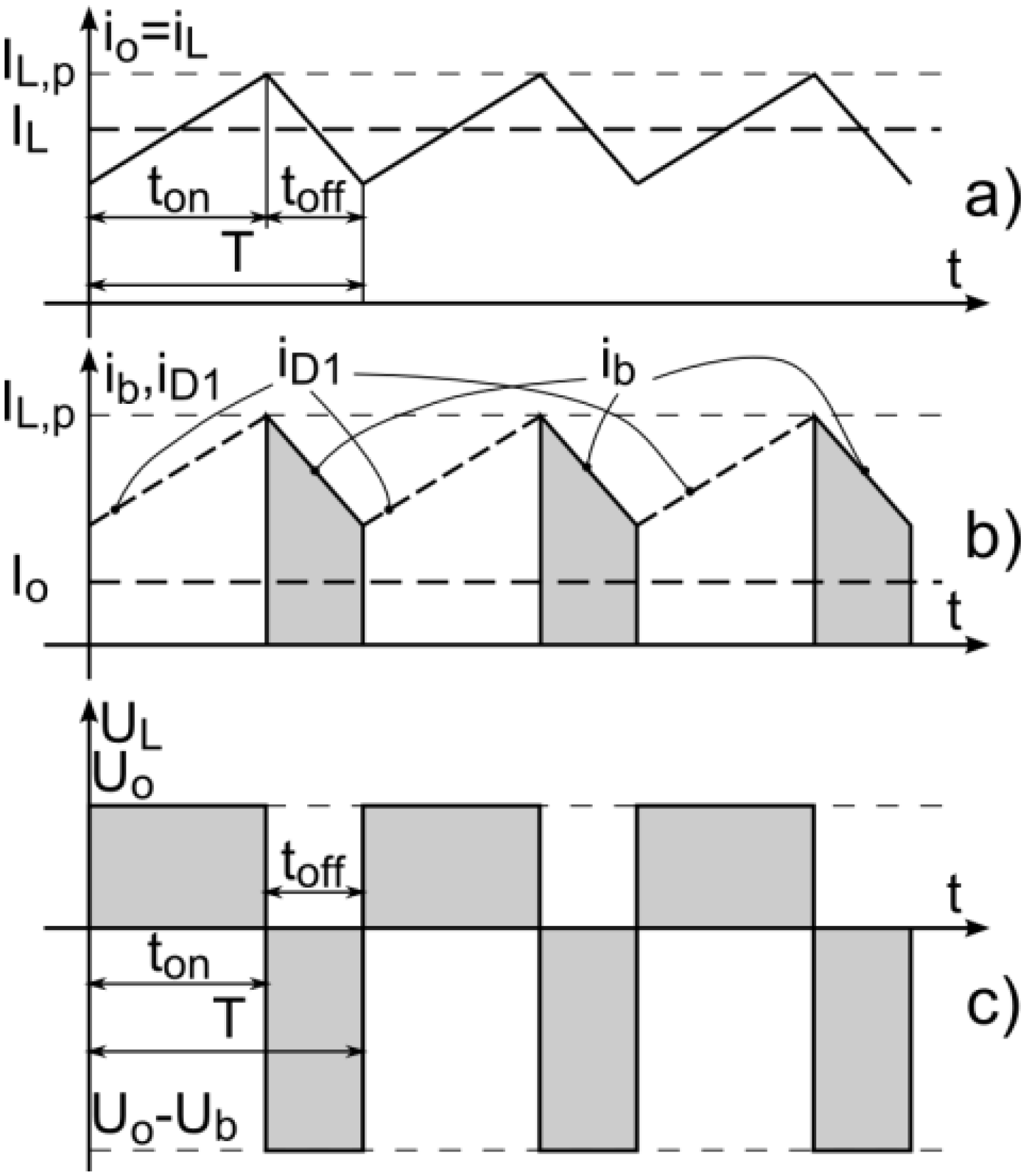
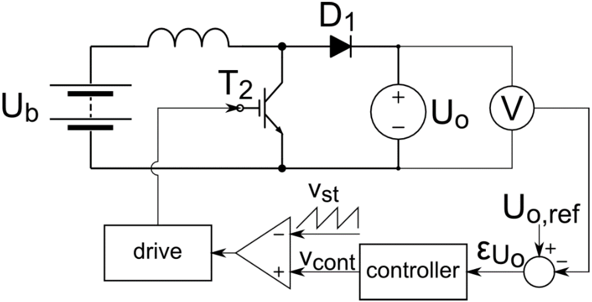
3. d.c.-d.c. Converter Control

Being Layout 1, as explained above, more convenient to interface an EESSS with an inverter, in the following, the analysis of Layout 1 is deepened to take into account the operation at discontinuous conduction mode.

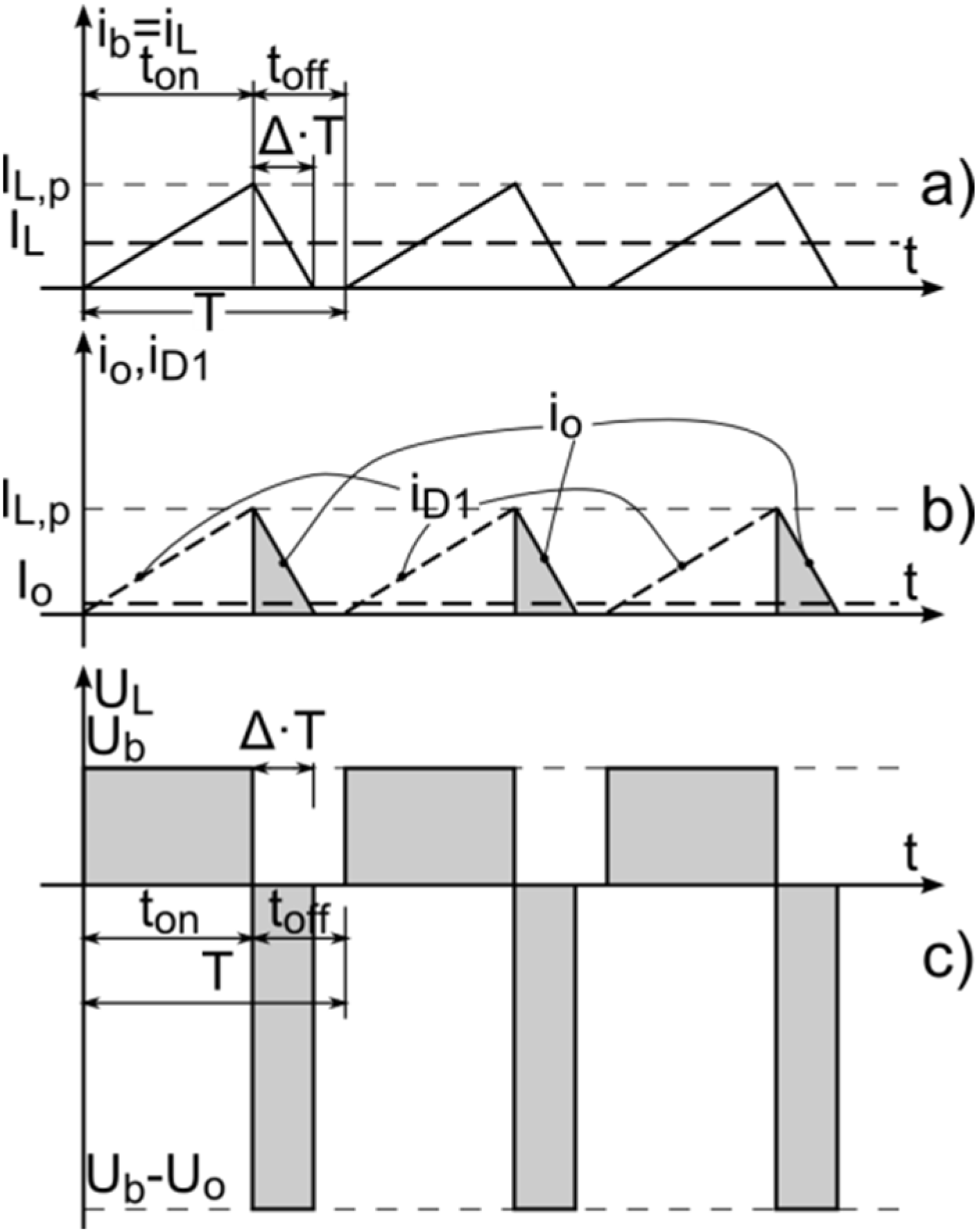
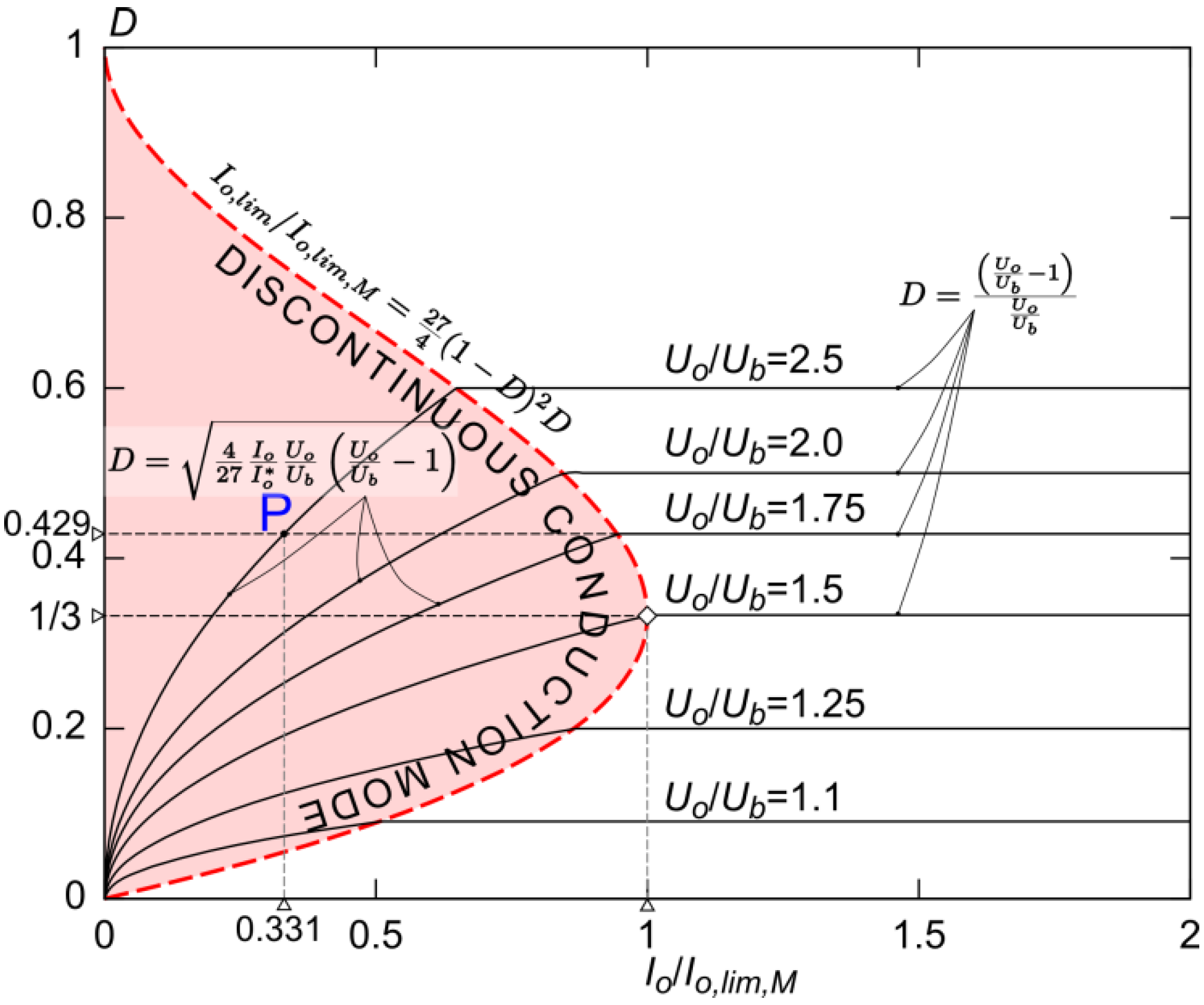
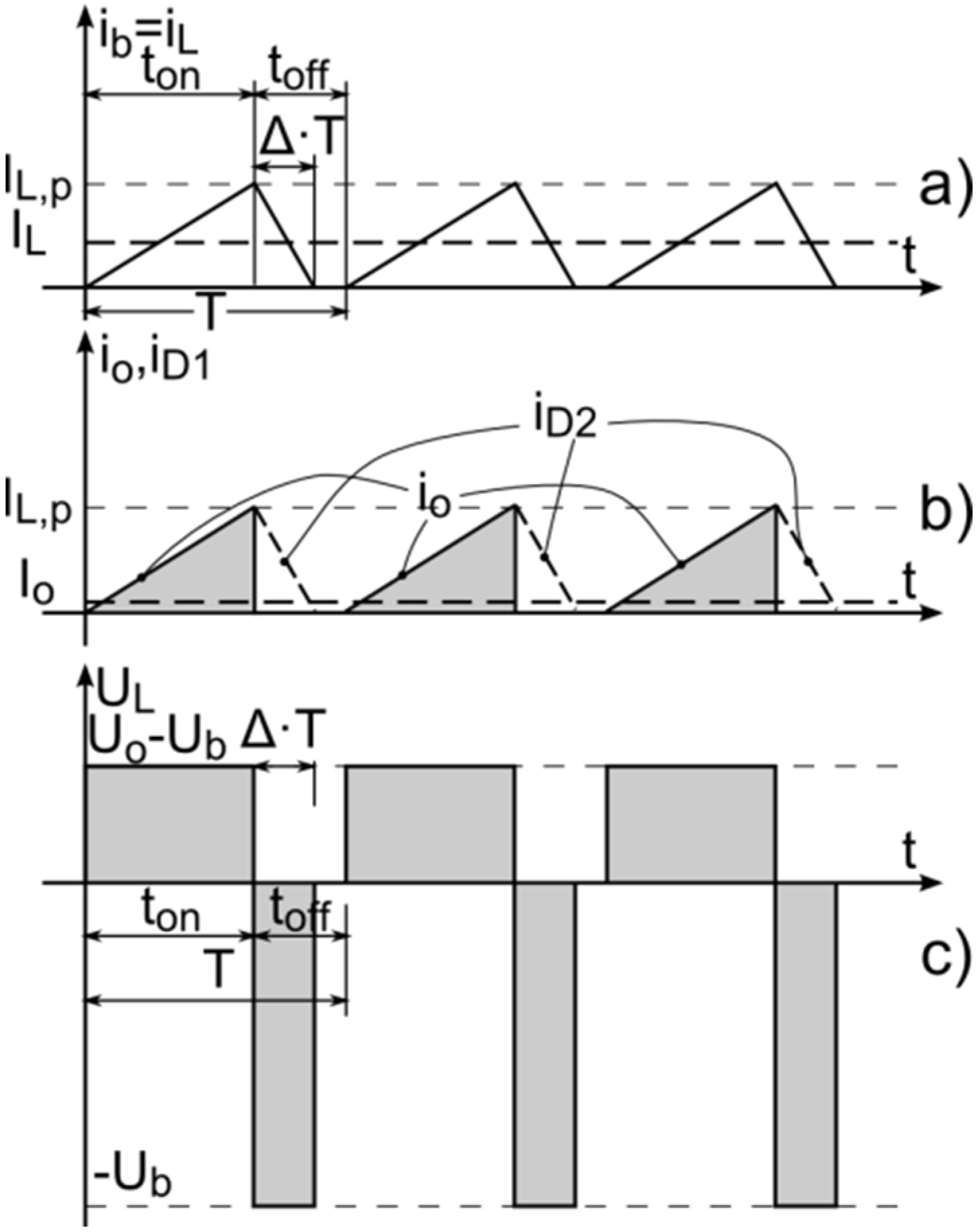
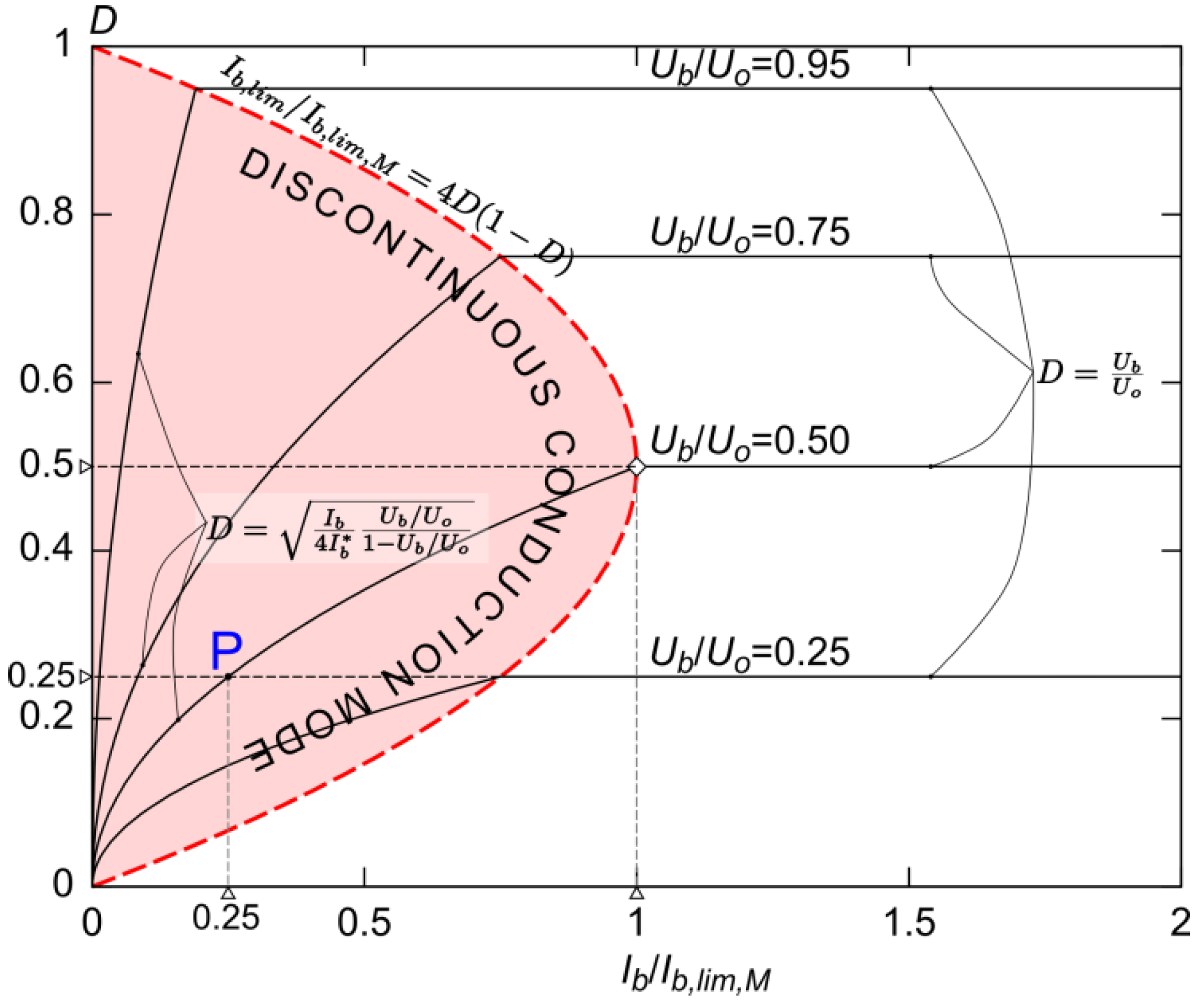
3.1. d.c.-d.c. Converter Control: Discontinuous Discharge Mode

With reference to Layout 1 of Figure 2a and to discharge operation, let us suppose that the average load current I_o is low enough to cause the zeroing of the inductor current i_L. The converter operates therefore in discontinuous discharge mode (see Figure 7).

Figure 7. Layout 1 discharge operation: current and voltage waveforms (discontinuous conduction).

Figure 7. Layout 1 discharge operation: current and voltage waveforms (discontinuous conduction).

In this condition [12] the converter output voltage does not depend only upon the T₂ duty cycle D but upon the supplied current I_o as well.

According to Figure 7, the average value of the supplied current is given by:

$$I_o=\frac{1}{T}{\displaystyle \underset{0}{\overset{T}{\int }}{i}_o}(t)dt=\frac{\text{Δ}\cdot I_{Lp}}{2}=\frac{\text{Δ}\cdot U_b\cdot D\cdot T}{2L}$$

(5)

Since the inductance net flux variation is null over the period T, it results:

$$U_{b}DT+(U_b-U_o)\cdot \text{Δ}\cdot T=0$$

(6)

and then, by solving (6) with respect to U_o, it results:

$$U_o=U_b\frac{D+\text{Δ}}{\text{Δ}}\ge U_b\frac{1}{1-D}$$

(7)

since it can be verified that $\left(D+\text{Δ}\right)/\text{Δ}\ge 1/\left(1-D\right)$ for 0 ≤ D ≤ 1; the transition from the continuous to the discontinuous mode corresponds to the limit condition Δ_lim = 1 − D. Inserting Δ_lim in Equation (5) and taking into account that Equation (1) still holds in the limit condition, so $U_b=\left(1-D\right)\cdot U_o$ can be substituted in Equation (5), the discontinuous limit current is obtained:

$$I_{o,lim}=\frac{{\left(1-D\right)}^{2}D\cdot U_o\cdot T}{2L}$$

(8)

Maximizing Equation (7) with respect to D, the maximum value I_o,lim,M is obtained for D_M = 1/3, i.e.:

$$I_{o,lim,M}=I_{o,lim}\left(D_M\right)=\frac{2U_o\cdot T}{27L}$$

(9)

then, Equation (8) can be rewritten as:

$$\frac{I_{o,lim}}{I_{o,lim,M}}=\frac{27}{4}{\left(1-D\right)}^{2}D$$

(10)

by replacing Equation (7) into Equation (5) and dividing by Equation (9), the average output current can be expressed as:

$$\frac{I_o}{I_{o,lim,M}}=\left(\frac{U_b^2\cdot D^2\cdot T}{2L(U_o-U_b)}\right)/\left(\frac{2U_o\cdot T}{27L}\right)=\frac{27}{4}{D}^2{\left(\frac{U_b}{U_o}\right)}^2(1-\frac{U_b}{U_o})$$

(11)

that, solved with respect to U_o, yields:

$$U_o=\frac{27D^2/2}{\sqrt{(27D^2+I_o/I_{o,lim,M})\cdot I_{o,lim,M}}-I_o/I_{o,lim,M}}\cdot U_b$$

(12)

whereas, solved with respect to D, it allows determining its value as a function of U_o/U_b and I_o/I_o,lim,M:

$$D=\sqrt{\frac{4}{27}\frac{I_o}{I_{o,lim,M}}\frac{U_o}{U_b}\left(\frac{U_o}{U_b}-1\right)}$$

(13)

According to Equation (12), in the discontinuous mode operation, since D is constant and by decreasing I_o, the output voltage exceeds the value given by Equation (1) and becomes higher and higher. For instance, Figure 8 shows that, for D = 42.9%, I_o/I_o,lim,M = 33.1% (point P in discontinuous mode operation), the voltage ratio U_o/U_b rises to 250% with respect to 175%, corresponding to continuous mode operation.

Figure 8. Layout 1 discharge operation: D as a function of current I_o/I_o,lim,M for different U_o/U_b values.

Figure 8. Layout 1 discharge operation: D as a function of current I_o/I_o,lim,M for different U_o/U_b values.

Figure 9. Outline of the feedback voltage control in discharge condition.

Figure 9. Outline of the feedback voltage control in discharge condition.

Figure 10. Elaboration of duty cycle control signal by a PWM technique.

Figure 10. Elaboration of duty cycle control signal by a PWM technique.

Provided that discontinuous conduction mode could occur at low load operation, output voltage regulation requires a feedback control of duty-cycle, outlined in Figure 9. The driving technique is based on the PWM approach, as it is represented in Figure 10: it can be easily verified that the switch duty cycle is D = t_on/T = v_cont/V_st, with v_cont and V_st control signal voltage and voltage peak value of a reference sawtooth wave v_st with period T.

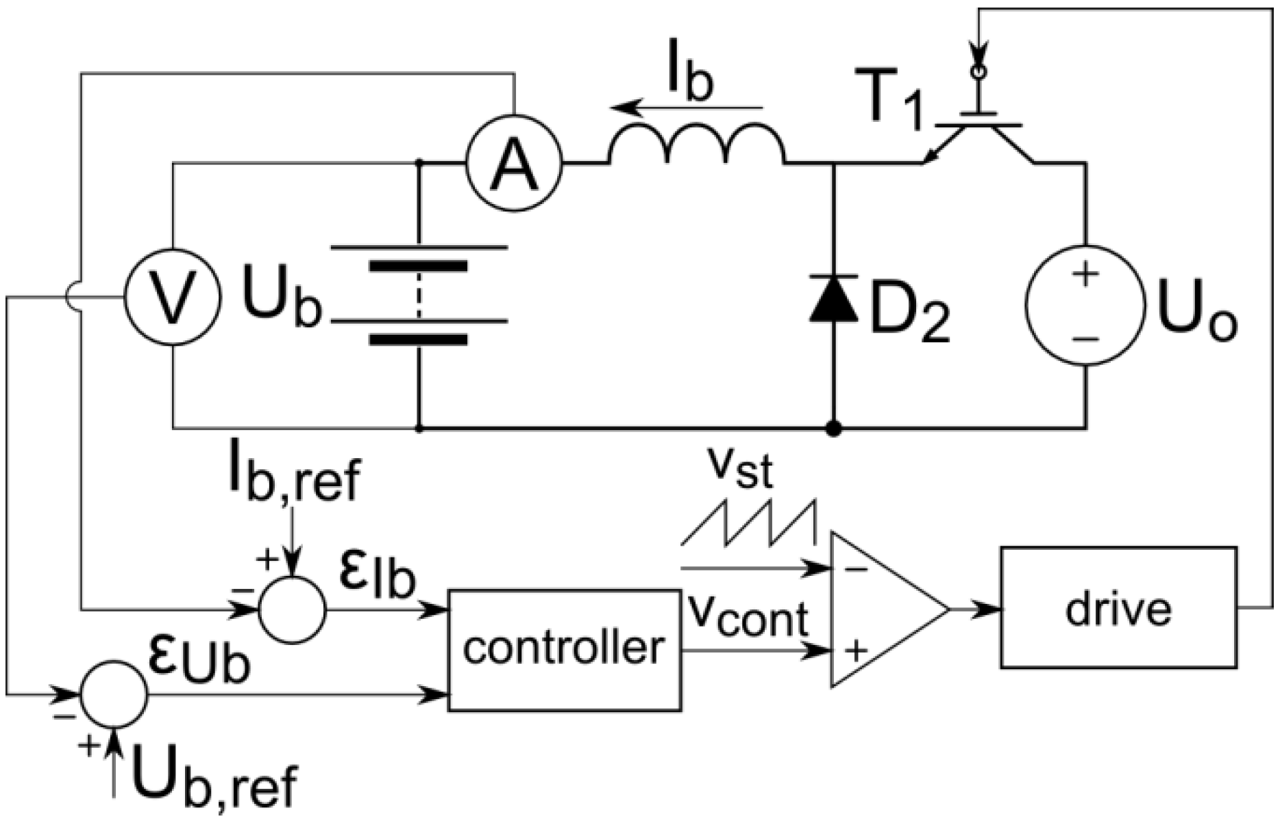
3.2. d.c.-d.c. Converter Control: Discontinuous Charge Mode

With reference to Layout 1 of Figure 2a and to discharge operation, let us suppose that the average current I_o flowing from the grid to the battery is low enough to cause the zeroing of the inductor current i_L. The converter operates therefore in discontinuous charge mode (see Figure 11) so that the converter output voltage depends upon both the T₁ duty cycle D and the input current I_o.

Figure 11. Layout 1 charge operation: current and voltage waveforms (discontinuous conduction).

Figure 11. Layout 1 charge operation: current and voltage waveforms (discontinuous conduction).

By imposing that the inductance net flux variation is null over the period T, it results:

$$-U_b\cdot \text{Δ}\cdot T+(U_o-U_b)\cdot DT=0$$

(14)

and then, by solving Equation (14) with respect to Δ:

$$\text{Δ}=\frac{U_o-U_b}{U_b}D=\left(\frac{1}{U_b/U_o}-1\right)D$$

(15)

By solving in turn Equation (15) with respect to U_b/U_o it yields (taking into account that Δ < 1 − D and 0 ≤ D ≤ 1):

$$\frac{U_b}{U_o}=\frac{D}{D+\text{Δ}}>\frac{D}{D+\left(1-D\right)}=D$$

(16)

The voltage ratio is higher than the corresponding value Equation (3) for continuous conduction mode. According to Figure 11, the average value of the current supplied from the converter to the battery is:

$$I_b=I_L=\frac{\left(D+\text{Δ}\right)\cdot I_{Lp}}{2}=\frac{\left(D+\text{Δ}\right)\cdot U_b\cdot \text{Δ}\cdot T}{2L}=D\cdot \text{Δ}\cdot U_o\cdot T/\left(2L\right)$$

(17)

Replacing in Equation (17) the duty cycle limit value Δ_lim = 1 − D, the current limit value corresponding to the transition from the continuous to the discontinuous conduction mode is obtained:

$$I_{b,lim}=D\cdot \left(1-D\right)\cdot U_o\cdot T/\left(2L\right)$$

(18)

By maximizing Equation (18) with respect to D, the maximum value I_b,lim,M is obtained for D_M = 1/2, i.e.:

$$I_{b,lim,M}=I_{b,lim}\left(D_M\right)=\frac{U_o\cdot T}{8L}$$

(19)

By solving Equation (17) with respect to Δ and taking into account (19) it yields:

$$\text{Δ}=\frac{I_b/I_{b,lim,M}}{4D}$$

(20)

The substitution of Equation (20) into Equation (16) gives U_b/U_o as a function of D and of I_b/I_b,lim,M:

$$\frac{U_b}{U_o}=\frac{D^2}{D^2+I_b/\left(4I_{b,lim,M}\right)}$$

(21)

Finally, the solution of Equation (21) with respect to D allows to express it as a function of U_b/U_o and I_b/I_b,lim,M:

$$D=\sqrt{\frac{I_b}{4I_{b,lim,M}}\frac{U_b/U_o}{1-U_b/U_o}}$$

(22)

According to Equation (21), in the discontinuous mode operation since D is constant and by decreasing I_b, the battery voltage U_b exceeds the value given by Equation (3) and gets closer and closer to U_o. For instance, Figure 12 shows that, for D = 25%, I_b/I_b,lim,M = 25% (point P in discontinuous mode operation), the voltage ratio U_b/U_o rises to 50% with respect to 25%, corresponding to continuous mode operation.

Figure 12. Layout 1 charge operation: D as a function of I_b/I_b,lim,M for different U_o/U_b values.

Figure 12. Layout 1 charge operation: D as a function of I_b/I_b,lim,M for different U_o/U_b values.

Hence, once again, a feedback voltage control is necessary, to regulate dynamically the duty cycle D, as it is shown in Figure 13, where a current control has been added, to regulate the battery charge current. The duty cycle is adjusted by a PWM technique, as mentioned in Section 3.1.

Figure 13. Outline of the feedback voltage control in charge condition.

Figure 13. Outline of the feedback voltage control in charge condition.

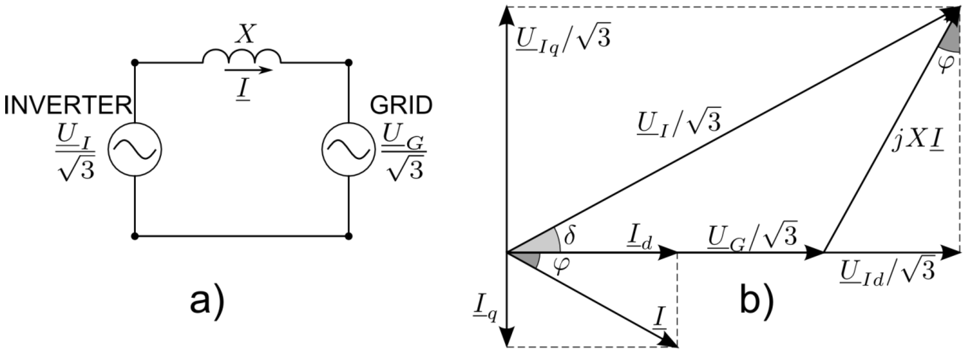
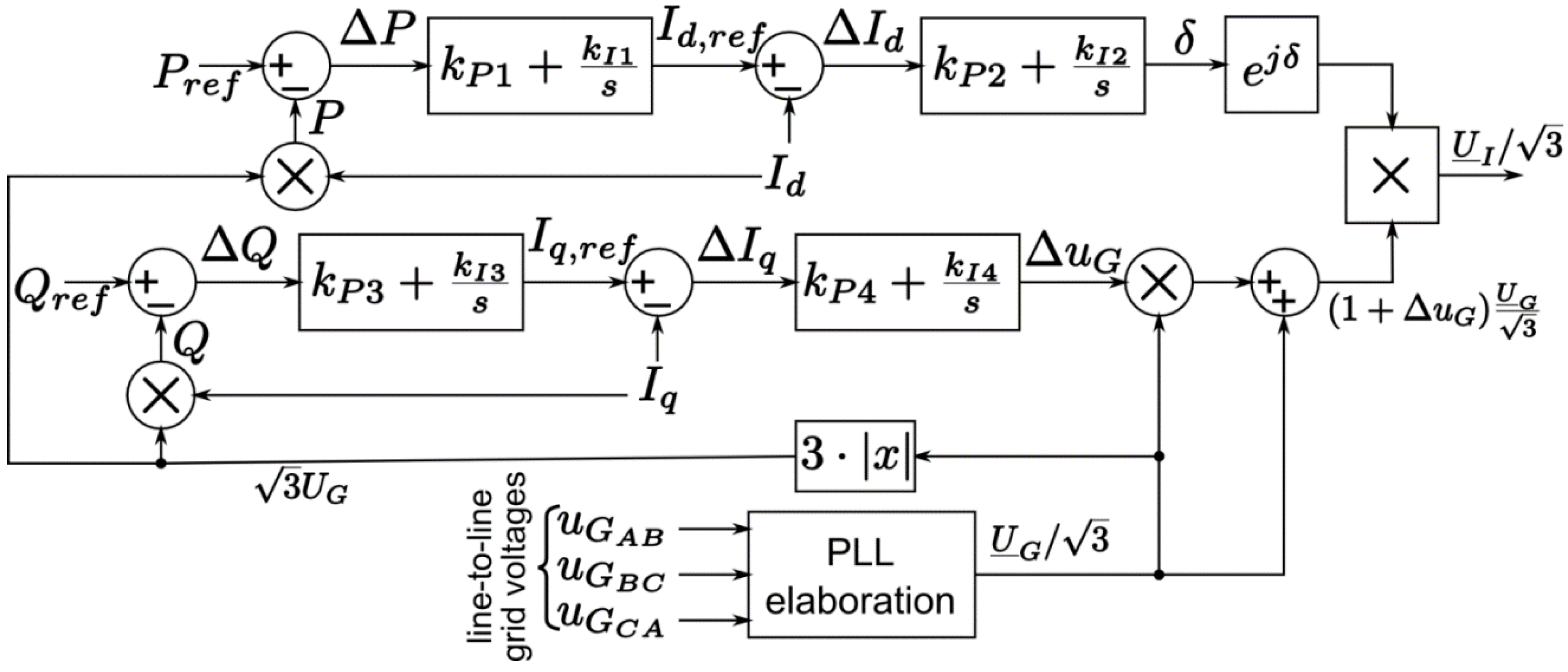
4. Full Bridge Inverter Control

The second conversion system in a two-stage inverter, is a full bridge inverter which as well as the a.c./d.c. current conversion has to control the flux of the active power and the reactive one from the EESSS to the grid and vice versa. The main control structures to regulate the power flux by means the full bridge inverter are presented in the following.

P/Q Control Structures

The power exchange between the inverter and the grid can be described by the simple equivalent circuit of Figure 14a.

Figure 14. (a) Inverter equivalent circuit; (b) Phasor diagram related to voltage and current components.

Figure 14. (a) Inverter equivalent circuit; (b) Phasor diagram related to voltage and current components.

The P/Q control strategy is the chief one for on-grid EESSS installations (conversely, V/f control is generally adopted for islanding operation). By means of simple geometric considerations on the phasor diagram of Figure 14b, related to the circuit of Figure 14a, the following equations can be derived:

$$\begin{array}{cc}{I}_d=I\text{cosφ}=\frac{U_{Iq}}{\sqrt{3}X}=\frac{U_I\text{sinδ}}{\sqrt{3}X}& I_q=I\text{sinφ}=\frac{U_{Id}-U_G}{\sqrt{3}X}=\frac{U_I\text{cosδ}-U_G}{\sqrt{3}X}\\ P=\sqrt{3}\hspace{0.17em}{U}_G{I}_d=\frac{U_G{U}_I\text{sinδ}}{X}& Q=\sqrt{3}\hspace{0.17em}{U}_G{I}_q=\frac{U_G\left(U_I\text{cosδ}-U_G\right)}{X}\end{array}$$

(23)

Assuming the angle δ to be small, approximations sinδ ≅ δ and cosδ ≅ 1 can be applied to Equation (23), which can be rewritten as:

$$P=\frac{U_G{U}_{I}sen\text{δ}}{X}\cong \frac{U_G{U}_I\text{δ}}{X};Q=\frac{U_G\left(U_I\text{cosδ}-U_G\right)}{X}\cong \frac{U_G\left(U_I-U_G\right)}{X}$$

(24)

According to Equation (24), active and reactive power flow can be managed adjusting inverter voltage phase displacement δ and amplitude U_I, respectively. Such quantities can be adjusted in turn according to the scheme outlined in Figure 15: the current errors ΔI_d and ΔI_q of the inverter current components I_d and I_q with respect to their reference values I_d,ref and I_q,ref are used as feedback signals to control δ and U_I respectively, according to first two equations in Equation (23), and consequently P and Q. Current reference values I_d,ref and I_q,ref are in turn obtained by elaborating active and reactive power errors ΔP and ΔQ of the actual power components P and Q with respect to their reference values P_ref and Q_ref. Of course, such strategy relies on the synchronization between the inverter. To such purpose, the grid phase voltage phasor U_G/$\sqrt{3}$, namely its amplitude and instantaneous phase, must be identified, by elaborating the grid voltage measurements u_GAB, u_GBC, u_GCA by a Phase-Locked Loop (PLL) technique [13]. Similarly, the actual inverter current components I_d and I_q with respect to the grid phase voltage reference frame are determined by the elaboration of the phase current measurements (not reported in Figure 15 for sake of clearness).

Figure 15. Outline of the P/Q control scheme.

Figure 15. Outline of the P/Q control scheme.

Assuming that other sources could contribute to the DC link, an alternative control strategy can be devised for the two-stage converter, aimed at providing stability and fast response at the same time coordinating the d.c./d.c. converter and the inverter operation. Accordingly, the former is driven to follow the active power reference to be injected at the d.c. link, whereas the latter is committed to following the reference value for the d.c. link voltage U_o, satisfying the reactive power demand at the same time.

5. Massive Energy Stationary Storage Experience in Italy

“Terna Storage” (a group of the Italian TSO Terna) has foreseen a massive installation (130 MW) of EESSS on the HV electric grid: at the moment, three 12 MW/12 MW/10.8 MW installations with sodium sulphide (NaS) [1,2,3,4,5,6] batteries for energy storage have been already installed. For these systems, the charge/discharge time is rather long, (i.e., 8 h), so that they have been named “energy intensive” or “energy-driven” (see Figure 16a). Another 16 MW installation has been realized with sodium nickel chloride [14] (see Figure 16b) and lithium-ion technologies with the aim of network services, which involves shorter charge/discharge times, so that they are called “power intensive” or “power-driven”.

Figure 16. (a) Terna Energy intensive EESSS installation in Ginestra, Italy; (b) Terna power intensive EESSS installation in Codrongianos, Italy.

Figure 16. (a) Terna Energy intensive EESSS installation in Ginestra, Italy; (b) Terna power intensive EESSS installation in Codrongianos, Italy.

The PCS configuration for the above mentioned installations are based on two-stage inverter, with voltage feed-back control. Thanks to the experience matured by the Italian industry on the inverter field related to the Photovoltaic plants, the nowadays inverter technology allows to reach very good performances. For the EESSS projects, Terna Storage standardized the inverter performances as it is reported in Table 2.

Table 2. Terna Storage standardized inverter performances.

Quantity	Range
Nominal efficiency	≥95.5%
Response time 0 ÷ 100%	≤80 ms
Phase inversion time (−100 ÷ 100%)	≤100 ms
Nominal load current THD	≤3%
Partial load (20%) current THD	≤5%
No-load Voltage THD	≤3%
Voltage regulation accuracy	±1%
Frequency regulation accuracy	±0.1%
Power regulation accuracy	±2%
Availability	≥99.5%

Table 2. Terna Storage standardized inverter performances.

Quantity	Range
Nominal efficiency	≥95.5%
Response time 0 ÷ 100%	≤80 ms
Phase inversion time (−100 ÷ 100%)	≤100 ms
Nominal load current THD	≤3%
Partial load (20%) current THD	≤5%
No-load Voltage THD	≤3%
Voltage regulation accuracy	±1%
Frequency regulation accuracy	±0.1%
Power regulation accuracy	±2%
Availability	≥99.5%

These values are referred to the complete system made by PCS and MV/LV transformer. The voltage total harmonic distortion (THD) and current one are sensibly better than the IEEE 1547 and IEC 61727 [15] prescriptions, which consider a THD ≤ 5% at the nominal load.

The availability of 99.5% is obtained by means of an inverter modular structure, with a redundancy of N-1 or higher. Consequently both the conversion system of the two-stage inverter (i.e., the d.c.-d.c. converter and the d.c.-a.c. one) consists of elements in parallel whose power ranges between 250 kVA and 500 kVA. With this configuration the fault of a single element (N − 1 fault condition) does not cause the operation interruption and the return of operation can be managed automatically. The fault of two components, (N − 2 fault condition) could involve a reduction of the power exchanged with the grid, but it does not involve the out of service of the entire system. Because of the high availability of the MT/BT transformer, a redundancy of it is not necessary and has not been foreseen.

6. Discussion and Conclusions

This paper aims at giving the readers a guide for the electrochemically stored energy conversion. The pros and cons of different conversion layouts have been analysed and the more suitable conversion architecture has been identified. For a safe operation of the entire system in case of discontinuous mode of the converter, a voltage control strategy have been presented. Moreover, the chief control scheme to regulate the active and reactive power exchange between the conversion system and the grid has been shown. The main aim of this work is to focus on the necessary elements which must be taken into account when a power conversion architecture has to be chosen, in the light of the PCS state of the art namely:

➢

The use of a two-stage converter is more convenient in order to avoid an oversized inverter. The first stage is made by a d.c.-d.c. converter, in order to maintain a constant continuous voltage reference for the inverter d.c. side. The second stage is represented by the d.c.-a.c. inverter itself;

➢

In order to avoid an impulsive behaviour of the battery current, the first stage of the two-stage converter has to be constituted by a layout 1 d.c.-d.c. converter;

➢

If the battery current is too low, the converter could work in discontinuous mode, so that the voltage references for the battery and the inverter cannot be controlled just by means of the converter piloting. Therefore, a feed-back voltage control is necessary to regulate the voltage reference in case of discontinuous mode;

➢

In order to regulate the active and reactive power exchange between the battery and the grid, it is possible to act on the inverter direct and quadrature current components by means of a suitable control system.

References

1. Andriollo, M.; Benato, R.; Dambone Sessa, S. 34.8 MW di accumulo elettrochimico di tipo ENERGY INTENSIVE mediante celle secondarie sodio-zolfo (Na-S). L'Energia Elettr. 2014, 91, 23–35. (In Italian) [Google Scholar]
2. Kawakami, N.; Iijima, Y.; Sakanaka, Y.; Fukuhara, M.; Ogawa, M.K.; Bando, M.; Matsuda, T. Development and field experiences of stabilization system using 34 MW NAS batteries for a 51 MW wind farm. In Proceedings of the 2010 IEEE International Symposium on Industrial Electronics (ISIE), Bari, Italy, 4–7 July 2010. [CrossRef]
3. Polgàri, B.; Hartmann, B. Energy storage for Hungary—NaS battery for wind farms energetics (IYCE). In Proceedings of the 2011 3rd International Youth Conference on Energetics (IYCE), Leiria, Portugal, 7–9 July 2011.
4. Roberts, B.P. Sodium-Sulfur (NaS) batteries for utility energy storage applications. In Proceedings of the 2008 IEEE Power and Energy Society General Meeting—Conversion and Delivery of Electrical Energy in the 21st Century, Pittsburgh, PA, USA, 20–24 July 2008. [CrossRef]
5. Garche, J.; Dyer, C.K.; Moseley, P.T.; Ogumi, Z.; Rand, D.; Scrosati, A.J.B. Preface. Encycl. Electrochem Power Sources 2009. [Google Scholar] [CrossRef]
6. Lu, N.; Weimar, M.R.; Makarov, Y.V.; Loutan, C. An evaluation of the NaS battery storage potential for providing regulation service in California. In Proceedings of the 2011 IEEE/PES Power Systems Conference and Exposition, Phoenix, AZ, USA, 20–23 March 2011. [CrossRef]
7. Monmasson, E. Power Electronic Converters: PWM Strategies and Current Control Techniques; Wiley-ISTE: West Sussex, UK, 2011. [Google Scholar]
8. Dos Santos, E.; da Silva, E.R. Advanced Power Electronics Converters: PWM Converters Processing AC Voltage; Wiley-IEEE Press: Hoboken, NJ, USA, 2014. [Google Scholar]
9. Chen, F.; Burgos, R.; Boroyevich, D.; Dong, D. Control loop design of a two-stage bidirectional AC/DC converter for renewable energy systems. In Proceedings of the 2014 Twenty-Ninth Annual IEEE Applied Power Electronics Conference and Exposition (APEC), Fort Worth, TX, USA, 16–20 March 2014. [CrossRef]
10. Cavalcanti, M.C.; Bradaschia, F.; Ferraz, P.E.P.; Limongi, L.R. Two-stage converter with remote state pulse width modulation for transformerless photovoltaic systems. Electr. Power Syst. Res. 2014, 108. [Google Scholar] [CrossRef]
11. Bnaei, R.M.; Salary, E. Application of multi-stage converter in distributed generation systems. Energy Convers. Manag. 2012, 62. [Google Scholar] [CrossRef]
12. Mohan, N.; Undeland, T.; Robbins, M.W.P. Power Electronics: Converters, Applications and Design; John Wiley & Sons Inc.: Hoboken, NJ, USA, 2002; ISBN 0471226939. [Google Scholar]
13. Nicastri, A.; Nagliero, A. Comparison and evaluation of the PLL techniques for the design of the grid-connected inverter systems. In Proceedings of the 2010 IEEE International Symposium on Industrial Electronics (ISIE), Bari, Italy, 4–7 July 2010. [CrossRef]
14. Benato, R.; Cosciani, N.; Dambone Sessa, S.; Lodi, G.; Parmeggiani, C.; Todeschini, M. La tecnologia sodio-cloruro di nichel (Na-NiCl2) per l'accumulo elettrochimico stazionario sulla rete di trasmissione. L'Energia Elettr. 2014, 91, 71–84. (In Italian) [Google Scholar]
15. International Electrotechnical Commission. Photovoltaic (PV) Systems—Characteristics of the Utility Interface, 2.0 ed.; IEC 61727; IEC: Geneva, Switzerland, 14 December 2004. [Google Scholar]