Article

Application of Displacement Height and Surface Roughness Length to Determination Boundary Layer Development Length over Stepped Spillway

1
School of Civil Engineering and Transportation, South China University of Technology, Guangzhou 510640, China
2
St. Anthony Falls Laboratory, Department of Civil Engineering, University of Minnesota, Minneapolis, MN 55112, USA
*
Author to whom correspondence should be addressed.
These authors contributed equally to this work.
Water 2014, 6(12), 3888-3912; https://doi.org/10.3390/w6123888
Submission received: 27 August 2014 / Revised: 12 November 2014 / Accepted: 24 November 2014 / Published: 12 December 2014

Abstract

:
One of the most uncertain parameters in stepped spillway design is the length (from the crest) of boundary layer development. The normal velocity profiles responding to the steps as bed roughness are investigated in the developing non-aerated flow region. A detailed analysis of the logarithmic vertical velocity profiles on stepped spillways is conducted through experimental data to verify the computational code and numerical experiments to expand the data available. To determine development length, the hydraulic roughness and displacement thickness, along with the shear velocity, are needed. This includes determining displacement height d and surface roughness length z0 and the relationship of d and z0 to the step geometry. The results show that the hydraulic roughness height ks is the primary factor on which d and z0 depend. In different step height, step width, discharge and intake Froude number, the relations d/ks = 0.22–0.27, z0/ks = 0.06–0.1 and d/z0 = 2.2–4 result in a good estimate. Using the computational code and numerical experiments, air inception will occur over stepped spillway flow as long as the Bauer-defined boundary layer thickness is between 0.72 and 0.79.

1. Introduction

Stepped spillways have gained interest for discharging excess flood water because of substantial energy dissipation along the chute due to the roughness of the steps. A sudden change in bed roughness occurs at the start of steps and the turbulent boundary layer of the steps generally begins at the crest of spillway and grows from the wall as the flow moves down the spillway, and eventually reaches the free surface. The inception point of air entrainment occurs shortly after the turbulent boundary layer of the stepped spillway approaches the free surface. The boundary layer development length was here defined from the crest to the inception point of air entrainment over stepped spillway. Many methods have been applied to estimate the location of the inception point over stepped spillways and there is the lack of an undisputed formulation [1]. The length on the spillway of non-aerated flow increases as the flow rate increases, with larger velocities that could cause unacceptable pressure fluctuations. Usually, determined by the size of steps and the flow discharge per width, the experimental studies, such as Chamani and Rajaratnam [2,3], Chanson [4,5], Cheng et al. [6,7], revealed three types of flows over a stepped spillway, namely, nappe flow, transition flow and skimming flow. For a given chute profile, the flow pattern may be either nappe flow at low flow rates, transition flow for intermediate discharge or skimming flow at larger flow rates. For a skimming flow, one of the most uncertain parameters in stepped spillway design is the length of boundary layer development.
Upstream of the inception point there is no air entrainment and the free surface is smooth, though some high- and low-frequency fluctuations are possible. At the step edges, the vertical velocity distribution in the turbulent boundary layer can be approximated by a power law [8,9,10,11], and data obtained in bed-roughened flows show that there is a region above the roughness layer where the smooth boundary upstream of the steps still adequately describes the vertical velocity distribution [12,13,14]. This transition boundary layer will be used to investigate and characterize the roughness parameters and the development of turbulent boundary layer.
Perry, et al. [15] used a deviation function introduced by Millikan [16] to the logarithmic velocity profile over a rough boundary using the displacement height d, relating to turbulent flow over rough surfaces. The customary logarithmic law for the velocity profile can then be expressed as,
u u * = 1 κ ln z + d z 0
where, u is the temporal mean flow velocity at a vertical distance z from the bottom; κ is the von Karman constant; u* is the bed friction velocity; d is the displacement height for the origin of the logarithmic profile and z0 is the surface roughness length.
Figure 1 illustrates a typical velocity profile in the non-aerated region of a stepped spillway, where H is flow depth; z is distance from origin of vertical profile of velocity; l is horizontal length of steps; h is height of steps (measured vertically); θ is angle between the pseudo-bottom formed by the step edges and the horizontal; ks is step dimension measured normal to the flow direction: ks = h × cosθ. The displacement height d appears in the logarithmic velocity profile for rough-wall turbulent boundary layers as a reference height for the bed-normal coordinate and should be taken as the level at which the average drag on the surface appears to act [17]. The surface roughness length z0 is a height-independent constant equivalent to that height above the roughness surface at which the flow velocity would go to zero if the logarithmic profile extended into the interfacial sub-layer. The local z0 value depends on the surface roughness characteristics. For many common types of surface covered roughness, d may be neglected or approximated accordingly. In flows over rough beds u*/κ, d and z0 can be found from a measured velocity profile, fitted by the logarithmic law [17]. For flow over a stepped spillway, the flow is highly turbulent, rapidly varied and there is a re-circulating vortex in the concavity of the steps, the displacement height d should be given a value in order to result in a good fit of velocity profiles.
Figure 1. Illustration of velocity profile on stepped spillway.
Water 06 03888 g001
This paper will develop relationships that can determine these three parameters (i.e., d, z0 and u*) to use in stepped spillway design and analysis. The objective is to first, calculate d and z0 from given velocity profiles in the developing turbulent boundary layer on stepped spillway and second, to establish a relationship between d and z0 with the variables describing the geometry and layout of a stepped surface, which may be more helpful to estimate the bottom shear stress and friction factor in practical applications, and third, to propose a new method to predict the distance from the crest to the air inception point over spillway flow, which may be more applicable for prediction of the inception point on stepped spillways of different slopes. In order to determine the boundary layer development length on skimming flow over stepped spillway, this paper adopted the first method described by Meireles et al. [1] to estimate the location of the inception point, i.e., visual observation of the cross section where there is a continuous presence of air within the flow at the sidewalls or within the step cavities.

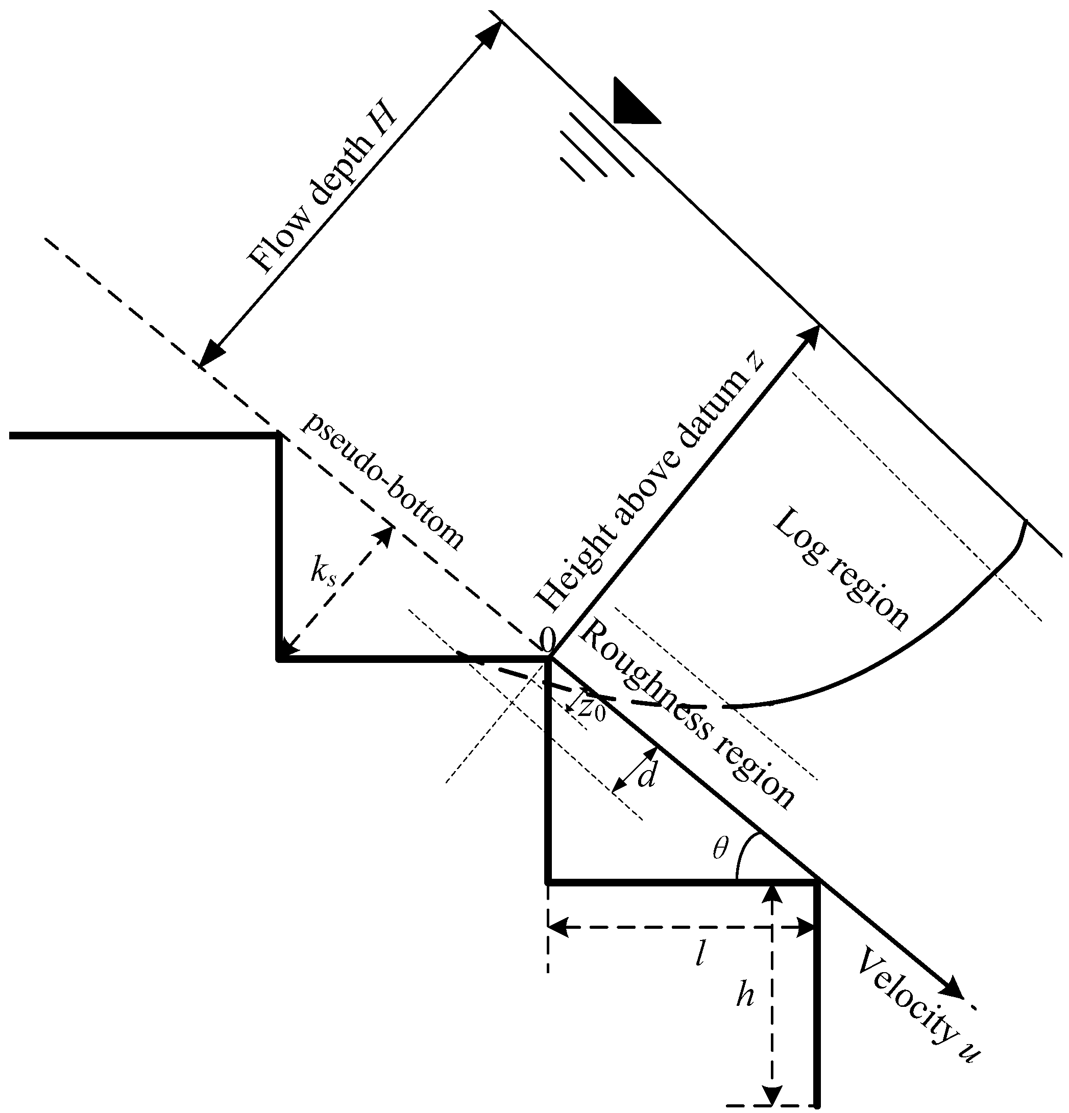
2. Methods to Calculate d and z0 from a Given Velocity Profile

To fit the logarithmic law to a velocity profile, three parameters u*/κ, d and z0 should be found from a velocity profile at five or more heights [17]. In many instances of open-channel flow, it was found that a logarithmic law can describe the velocity profile in the bottom 15% of the flow depth [18], 20% [19], 50% [20] or 75% [13]. Thus there is not an explicit standard for the flow heights on the estimation of u*, d and z0 using a fitted logarithmic profile. For the wall layer of open-channel flows, the von Karman constant κ will be assumed to have the universal value 0.41, regardless of the Reynolds and Froude numbers [19].
The displacement height d over rough surfaces has been investigated over vegetation [21,22], roughness in pipe flows [15,23] and forest canopies [24,25]. The technique of Perry et al. [15] is used for most flow conditions, where arbitrary values of d are added to the wall distance measured from the top of the roughness elements until a straight line occurs in semi-log space in the log-law region. The value of d that results in this straight-line fit is then considered to be the displacement height.
When calculating estimates of u*, d and z0 from velocity profiles, it is advised to regress u against ln(z + d) as opposed to ln(z + d) against u, to calculate values of friction velocity u* and surface roughness length z0 [26]. Measured values of u are generally observed with greater error than ln(z + d).
Yu and Tan [27] and Bergstrom et al. [28] did not consider the velocity profile located at the immediate vicinity of a roughness element (i.e., z < 0.1 δ, δ is turbulent boundary layer thickness) to fit d, u* and z0. In this paper the velocities at the immediate vicinity of the wall or the roughness elements, i.e., z < 0.1 δ, were also not considered in the profile matching to obtain d, u* and z0.
To determine the displacement height d, the velocity profiles are plotted as u versus ln(z + d). The value of d is incremented or reduced by 1 mm [29] and a straight-line fit determined by a least-squares regression is applied to the resulting points. The fit is judged by the standard error of the estimate, SE, or the square of the correlation coefficient, R2.
Figure 2 provides the plot used to determine the displacement height d under one of the typical velocity profile, where the velocity profile is located in the middle vertical section and from the tip of the step normal to the water surface in the nonaerated skimming flow zone on a stepped spillway. The d can be determined when the velocity profile in the logarithmic region is the closest to a straight line on this semi-log plot. Figure 3 illustrates the SE corresponding to different values of d. When the displacement height d is not considered (i.e., d = 0), the relationship between the temporal mean velocity profile against ln(z) is a curve, instead of a straight line. Then, the normal distance z, where z > 0.1 δ, is adjusted by changing d until the curve approaches a straight line. Along with the increased d, the coefficient of determination R2 is increased. The value of SE is decreased to reach a minimum value then increased at larger values of d (seen from Figure 3). It can therefore be said that the value of d corresponding to the minimum SE is the best estimate in the log-law region of velocity profile. As seen from the Figure 2 and Figure 3, the value d of the best fit is 0.016 m or 0.017 m.
Figure 2. Determination the displacement height d under one of the typical velocity profiles in the nonaerated skimming flow zone on a stepped spillway.
Water 06 03888 g002
Note: The physical model with a standard U.S. Army Corps of Engineers profile consisted of 13 steps. The first five steps were transition steps and the height of each is 2, 2.4, 3, 4, and 5 cm. Below eight steps, the height = 6 cm, the width = 4.5 cm, continued down to the toe. The spillway slope was 53° and the specific discharge was 0.1 m2/s. The location of inception of free-surface aeration was at step 10.
Figure 3. Standard error at various values of d.
Water 06 03888 g003

3. Simulation of Velocity Profile on Stepped Spillways

In order to achieve the relationships between d, z0 and geometries of stepped spillways, it is important to obtain abundant velocity profiles under different geometries. Taking a collection of measurements on stepped spillways from publications [30,31,32,33,34,35], the measured velocity data are primarily focused on the region downstream of air inception. There are also limitations related to slopes or geometries of stepped spillways. However, a well-verified computational fluid dynamics (CFD) equation solver can incorporate many different geometries and discharges, and is capable of eliminating the shortcomings of insufficient experimental data.
A CFD model complements experimental and theoretical fluid dynamics by providing an alternative cost-effective means of simulating real flows. Substantive CFD research has been conducted for simulation of flow over a stepped spillway, especially for the flow field upstream of the air entrainment inception, e.g., [36,37,38,39,40,41,42,43,44,45]. In this paper, the commercial software Fluent 6.2 [46] was used to process the numerical simulation. Due to the identity of spillway width and the ratio of spillway width to water depth being large enough with no reflection of side-walls to the flow field, the numerical model is based on the 2D Reynolds averaged equations, where the free-surface is represented using the refined volume-of-fluid algorithm, the turbulence is represented by a renormalization group (RNG), and the k-ε closure model is used for characterizing the flow over stepped spillways.
A refined volume-of-fluid algorithm is applied to track the free surface. A single set of momentum equations is shared by air and water. In each calculated cell, the sum of the volume fractions of air and water is unity. The tracking of the interface between air and water is accomplished by the solution of the continuity equation with the following Equation,
α w t + u i α w x i = 0
The value of αw in a cell represents the fractional volume of the cell occupied by water. The free surface is defined by a value of αw = 0.5, which is a common practice for volume fraction results [46].
The density and viscosity in the above equations are calculated by weighted average method, that is,
ρ = α w ρ w + α g ρ g
μ = α w μ w + α g μ g
where αg is the fractional volume of the cell occupied by air; ρw and ρg are the density of water and air; μw and μg are the viscosity of water and air, respectively.
The simulated domain was divided into unstructured grids that had a high adaptability to the complex geometry and boundary. Near the spillway wall the adjacent grids were at non-dimensional wall distances of 30 < Y+ = u*z/ν < 300 (0.1–0.7 mm), where ν is kinematic viscosity. The convective fluxes in the mean volume fraction, momentum and turbulence closure equations were discretized by employing a conservative, second-order accurate upwind scheme. The pressure-velocity coupling algorithm is the pressure-implicit with splitting of operators (PISO). A time step less than or equal to 0.001 s was selected. Convergence was reached when the normalized residual of each variable was on the order of 1 × 10⁻³. The degree of agreement for the lower part of the velocity profiles is dependent on the wall function. The experimental velocity profiles agreed better with the numerical results when the non-equilibrium wall function were applied, which were in accordance with the research results of Bijan [47] and Carvalho and Martins [38].

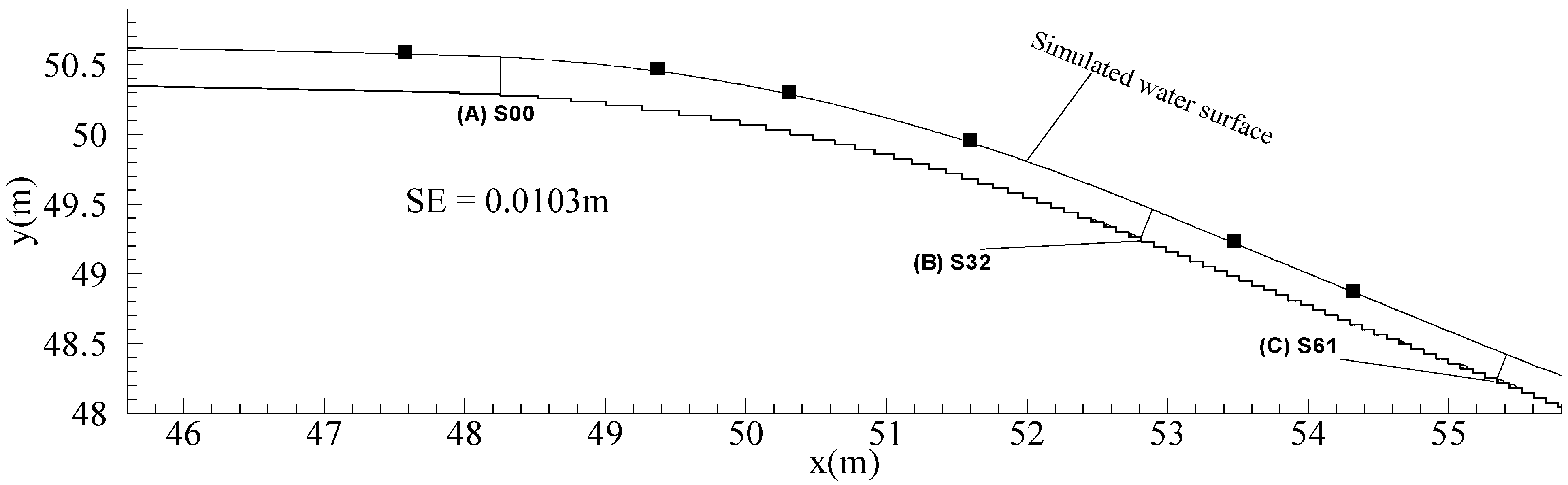
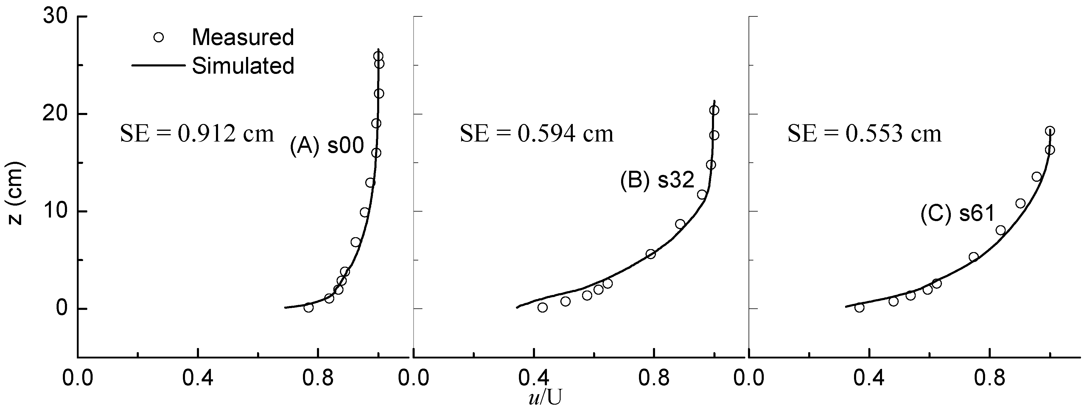
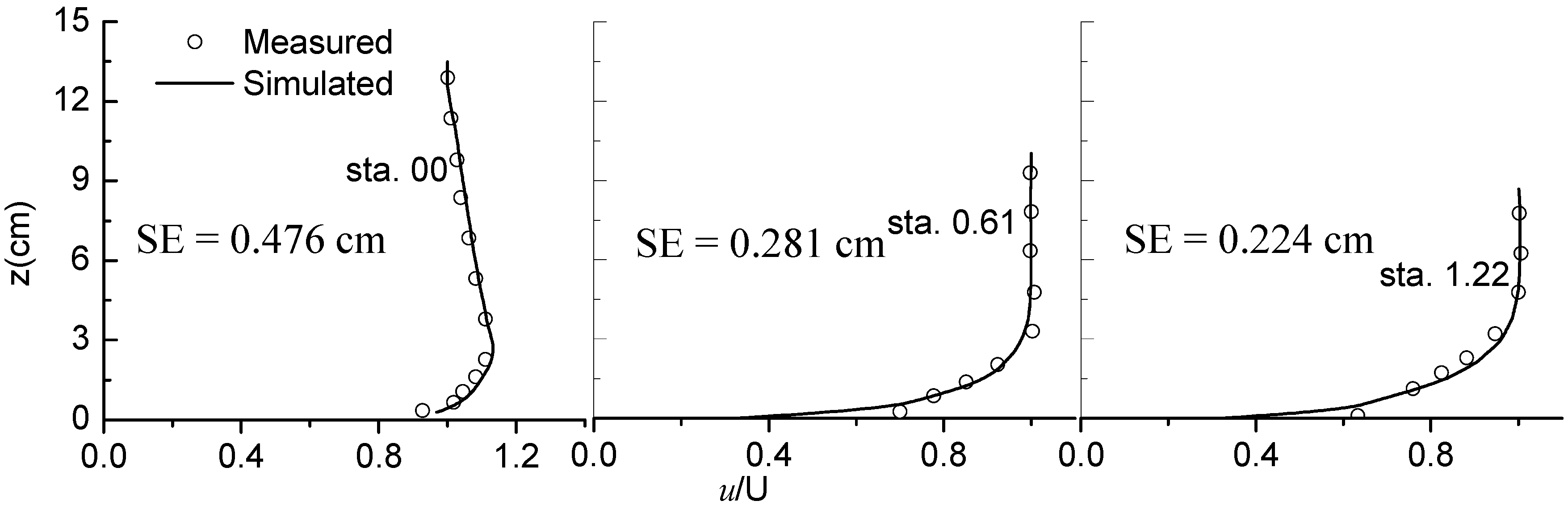
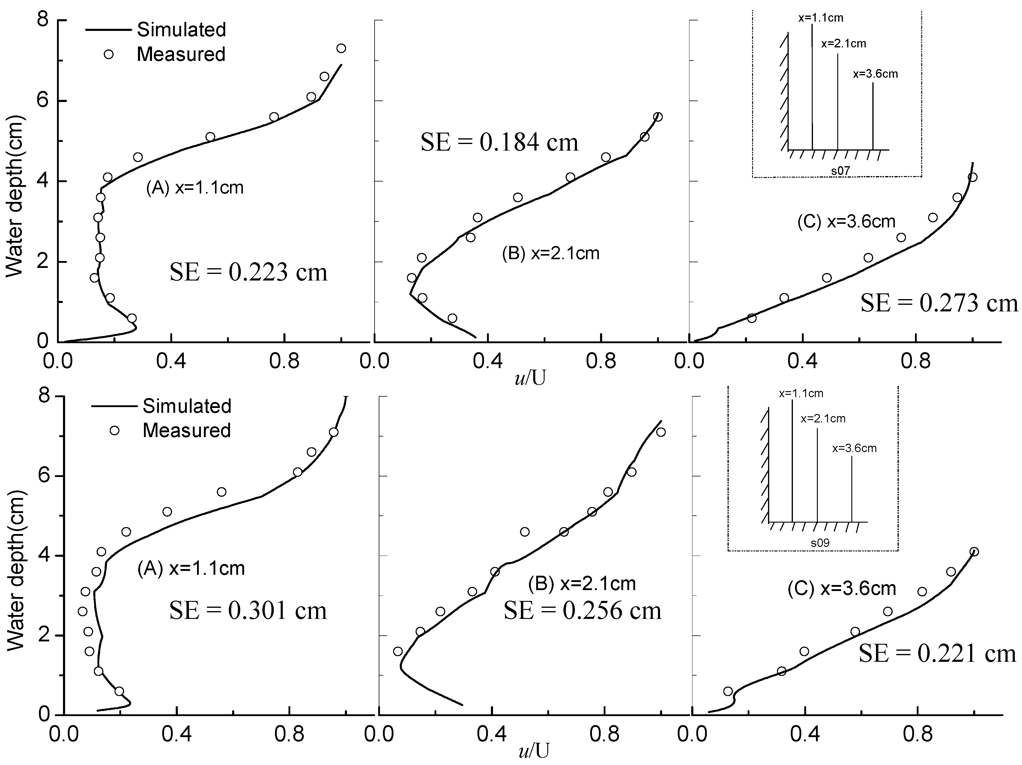
4. Verification of Simulated Velocity Profiles

Measured velocities and water depth from the physical models of Lueker et al. [48], Hunt and Kadavy [49] and Chen [41] were chosen to verify the above-mentioned CFD methods with a wide range of spillway slope. Lueker et al. [48] measured three velocity profiles and six water surface elevations in the non-aerated flow region with a spillway slope of 21.8° and a specific discharge of 0.9 m2/s. Hunt and Kadavy [49] measured three velocity profiles before the air inception with a spillway slope of 14° and a specific discharge of 0.28 m2/s. Chen [41] measured velocity profiles within two steps before the air inception with a spillway slope of 53° and a specific discharge of 0.1 m2/s. More detailed physical model descriptions are given in Table 1.
Table 1. Experimental investigations of skimming flow over stepped spillway.
ReferenceSpillway Geometry DescriptionsFlow Conditions
[48]Physical model with an ogee profile was 40.2 m long and 2.74 m wide, consisting of a 23.46 m long rectangular chute at a 2% slope ending with a stepped spillway, which then dropped 2.35 m into a stilling basin. Stepped spillway including 68 steps initially followed a parabolic ogee path and became linear at a slope of 21.8° about half way along the spillway.Q = 2.46 m3/s
No obvious air entrainment over the steps.
[49]Physical model was 10.82 m long and 1.8 m wide, consisting of a 2.44 m long broad chute ending with a stepped spillway, which then dropped 1.52 m into a stilling basin. Stepped spillway including 40 identical steps (step height = 3.8 cm, width = 15.2 cm) became at a slope of 14°.Q = 0.504 m3/s
The inception point was located at the distance of 3.44 m from the first step.
[41]Physical model with a standard U.S. Army Corps profile consisted of 13 steps. The first five steps were transition steps and the height of each is 2, 2.4, 3, 4, and 5 cm. Below eight steps (height = 6 cm, width = 4.5 cm) continued down to the toe. The spillway slope was 53°.Q = 0.03 m3/s
The location of inception of free-surface aeration was at step 10.
The free surfaces measured by Lueker et al. [48] are shown with the simulation results in Figure 4. The flow velocity profiles of s00, s32 and s61 (shown in Figure 4) are plotted in Figure 5, where U is the free-stream velocity, the points represent measurements and the solid lines are from the simulation. The simulated water surface agrees well with that of the measurements.
The comparison of velocity between simulation and measurements in Hunt and Kadavy [49] are shown in Figure 6, where the measured velocity profiles were taken normal to the pseudobottom of the spillway and the sections are located at the distances from spillway crest of 0.0, 0.61 and 1.22 m, respectively. The simulations and measurements correspond except for a discrepancy near the pseudobottom of the spillway. At these locations there are interactions between the clockwise eddy below the steps and skimming flows near the pseudo-bottom, and it is difficult to measure the local water velocities accurately. The lack of a perfect agreement could be due to either the simulation or the measurements.
Figure 7 shows the velocity distributions at different sections of step No. 7 and 9 in Chen [41], where x = 1.1, 2.1 and 3.6 cm represent the linear distance from the concave of step to the section respectively. At x = 1.1 and 2.1 cm, the measurements are within the shadow of the step, which is a notoriously difficult location to simulate flow velocity [50]. The simulated velocities are in agreement with the measurements.
Figure 4. Water surfaces obtained by simulation and measurement in Lueker et al. [48].
Water 06 03888 g004
Figure 5. Velocity obtained by simulation and measurement in Lueker et al. [48].
Water 06 03888 g005
Figure 6. Velocity obtained by simulation and measurement in Hunt and Kadavy [49].
Water 06 03888 g006
Figure 7. Velocity obtained by simulation and measurement in Chen [41].
Water 06 03888 g007
The standard error of the estimate:
SE =  r = 1 n ( φ r φ r ) 2 n
where r is the data point of the vertical profile, φr is the corresponding measured value at the point r, φ r is the estimated value of φr, n is the number of measured points, is also presented in Figure 4, Figure 5, Figure 6 and Figure 7. Seen from the Figure 4, the value of SE was 0.0103 m, indicating the mean error of water surface levels between experiments and simulations was about 1 cm. Seen from Figure 5, Figure 6 and Figure 7, the mean error of water depth corresponding to the non-dimensional variable u/U was small, relative to the water depth. The simulation errors closest to the step edges were a little bigger; where the maximum error was about 25%.
Though there exists the maximum simulation error of 25% compared to the measured velocity values, one must consider the difficult measurements on the velocity profiles closest to the step edges. For this analysis of mean velocity profiles and development length, there is little that can be gained by shifting to a three dimensional simulation. The numerical experiments will be discussed in the next Section.

5. Numerical Experiments on Stepped Spillways

Based on the original physical models from Lueker et al. [48], Hunt and Kadavy [49], Chen [41], Carosi and Chanson [51] and Felder and Chanson [52], numerical experiments were designed to simulate a realistic range of stepped spillways flows by changing the slope, discharge or intake Froude number. The conditions of each numerical experiment are listed in Table 2, where q is the discharge per unit width; θ is the slope of stepped spillway; Fr-in is the initial gate Froude number (=u0/(9.81H0)); u0 is the initial average velocity; H0 is the initial water depth; Li-exp is the distance from the crest to the inception point of air entrainment on stepped spillway supplied by the literatures; M is the Charnock constant derived from Charnock [53].
Table 2. Conditions of each numerical experiment.
SourceRun No.h (m)l (m)ks (m)q (m2/s)θ (deg)Fr-inLi-exp (m)M
[41]10.0600.0450.0360.10053.20.0570.5912.652
20.0600.0680.0450.10041.70.057-11.498
30.0300.0450.0250.10033.70.057-11.806
40.0600.0900.0500.10033.70.057-10.528
50.0600.0450.0360.06753.20.0410.4411.531
[49]60.0380.1520.0370.28014.013.4415.035
70.0380.1520.0370.42014.014.5411.673
80.0380.1520.0370.62014.01-12.998
90.0380.1520.0370.82014.01-13.855
100.0760.3040.0740.82014.01-10.205
110.0760.1520.0680.82026.61-14.310
[48]120.0350.0870.0320.89921.82.26-19.149
130.0350.0870.0320.89921.81-19.925
140.0350.0870.0320.89921.80.674-18.275
150.0350.1370.0340.89914.32.26-18.451
160.0350.2270.0350.8998.72.26-18.981
[51]170.1000.2500.0990.14321.80.0581.626.171
[52]180.0500.1250.0500.14721.80.042.028.529
Notes: “-” means there is no physical measurement and should be obtained by numerical simulations.

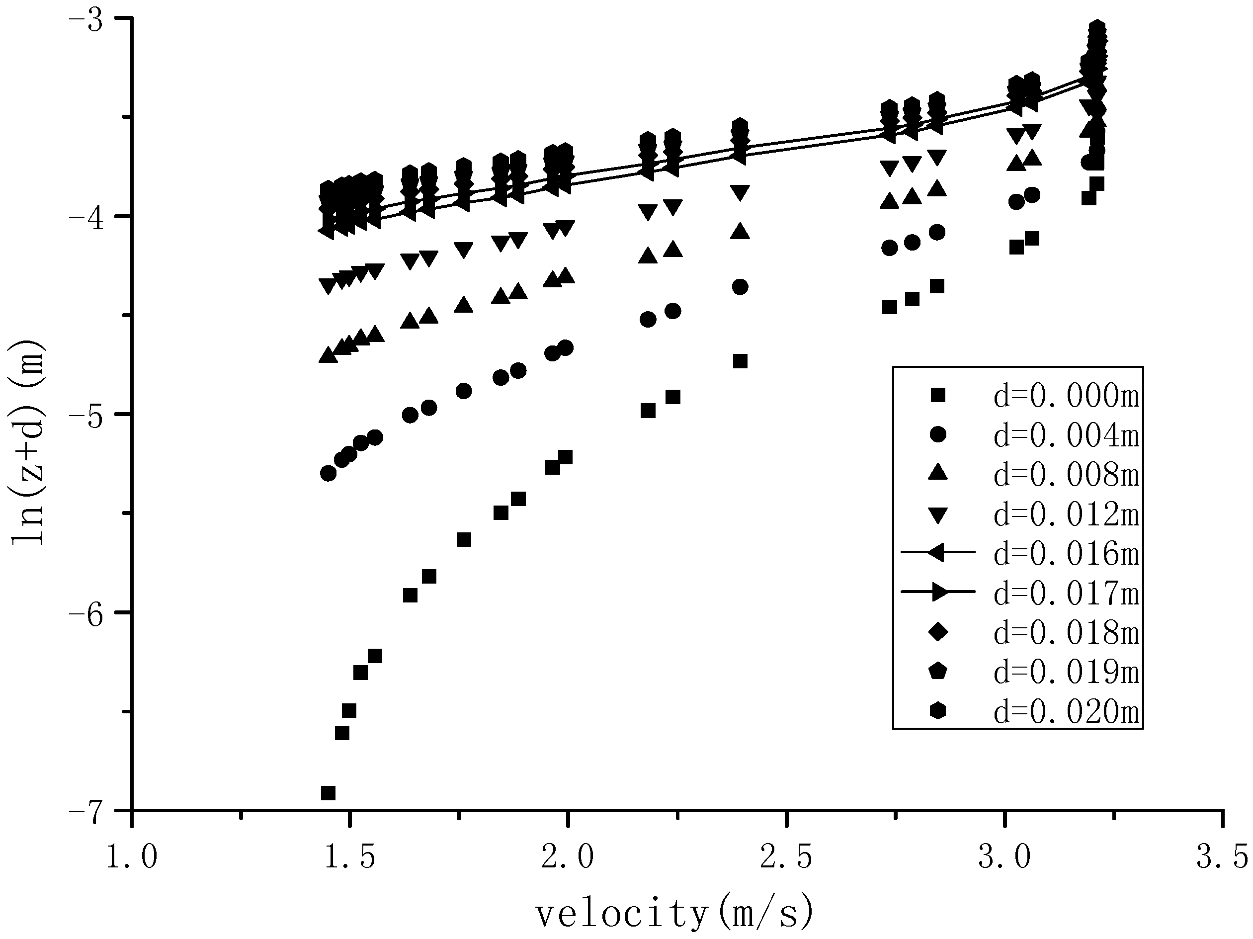
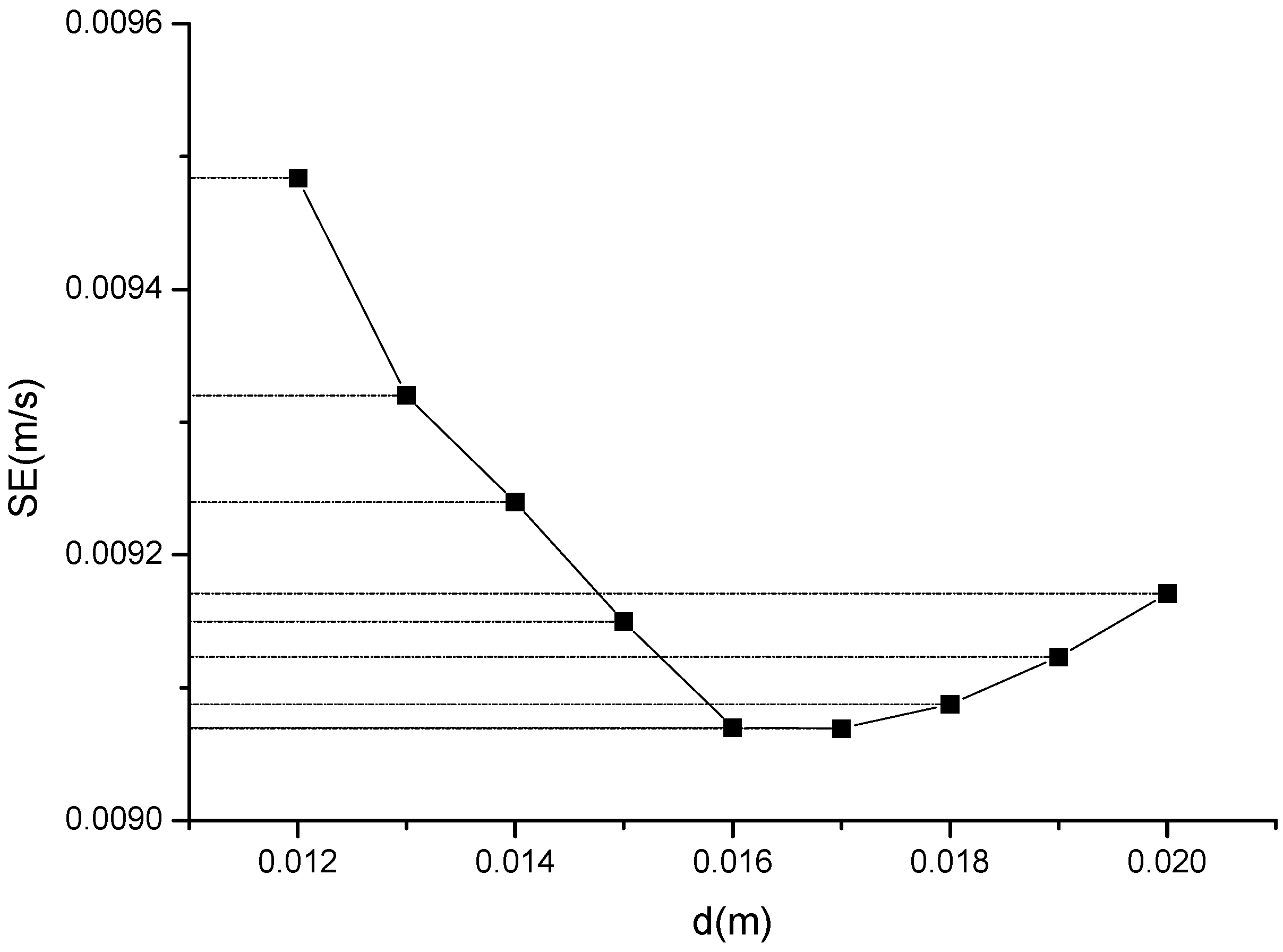
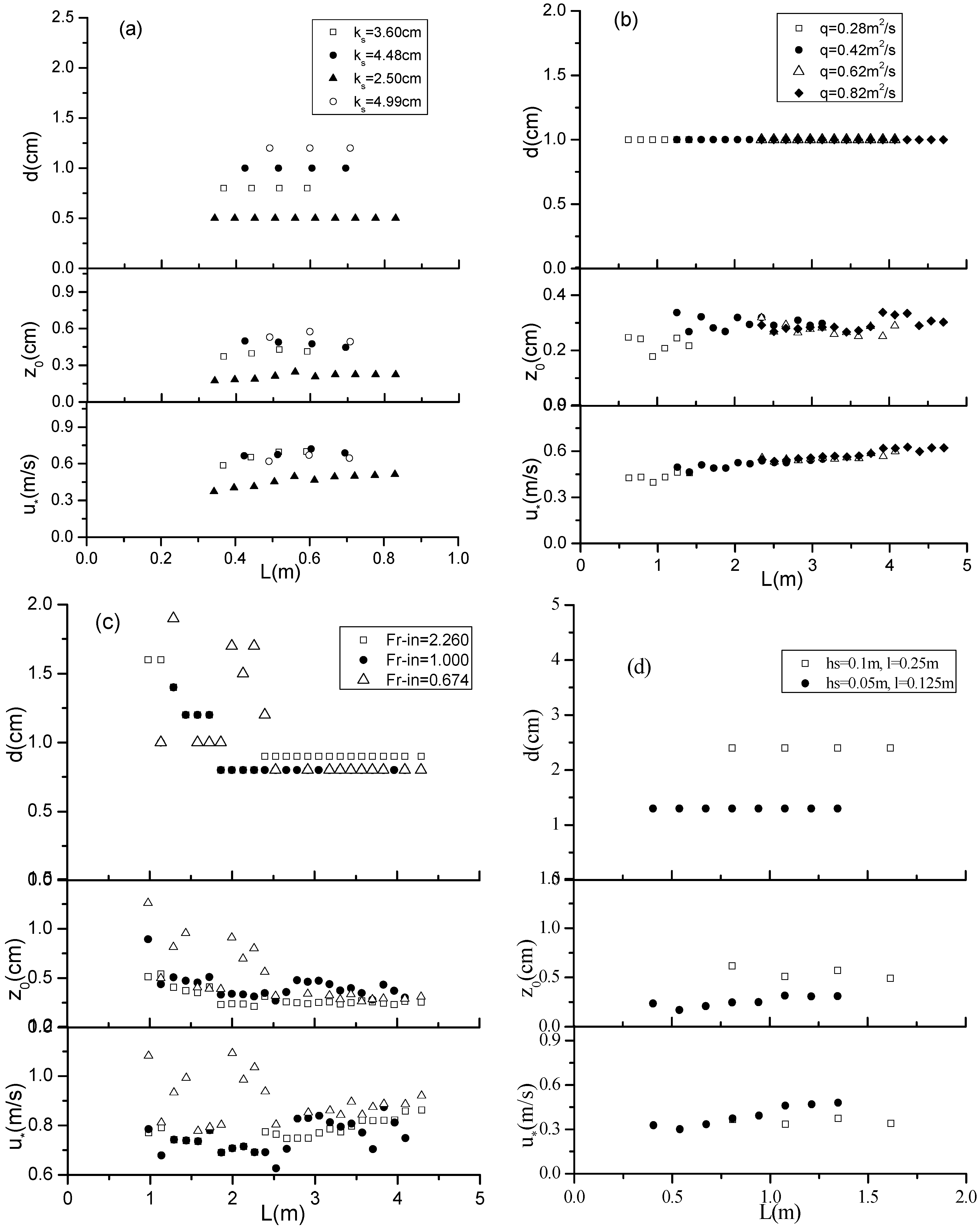
5.1. Estimates of the Displacement Height, Surface Roughness Length and Friction Velocity

Using the method provided in Section 2, estimates of d, z0 and u* were obtained from simulated velocity profiles of the 18 runs. Under the different conditions of ks, q and Fr-in, the results for d, z0 and u*, shown in Figure 8, are plotted against the distance down the stepped spillways. Figure 8a illustrates the estimates of d, z0 and u* when the roughness height ks is changed, and the discharges per width and Froude number of intake are unchanged. It shows that d and z0 are dependent on ks and a larger ks results in a larger d or z0, as expected. Figure 8b illustrates the estimates of d, z0 and u* when all of hydraulic conditions except the discharge per unit width are unchanged. It indicates that neither d, z0, nor u* is a function of discharge per unit width. Figure 8c provides the effect of initial gate Froude number on d, z0 and u* under the conditions of similar discharges. When the Fr-in is set to 2.26 or 1, the flow is supercritical from the intake to the end of the spillway. When the Fr-in is set to 0.674, the flow is subcritical at the beginning of the stepped spillway and then transforms to supercritical flow along the spillway. The results indicate that d, z0 and u* have nearly independence on Fr-in. There is some scatter about d and z0 in the boundary layer development region, before 2.5 m on spillway, the reason will be explained in the next section. After this region, the d, z0 and u* settle to approximately 0.75 cm, 0.25 cm and 0.9 m/s, respectively. Figure 8d provides the estimates of d, z0 and u* when the step height and length are doubled. It shows that the estimates of d and z0 are nearly doubled as well. Seen from the Figure 8a–d, the results suggest that the estimates of d or z0 are close to constant with distance down a stepped spillway when its slope is constant, which indicates d or z0 is not proportional to the boundary-layer thickness. The friction velocities have a slight increase with distance down the stepped spillway, which occurs because, as the turbulent boundary layer grows, the depth increases while the energy grade line is still close to that of the spillway.
Figure 8. Estimates of d, z0 and u* for the numerical experiments: (a) from run 1, 2, 3 and 4; (b) from run 6, 7, 8 and 9; (c) from run 12, 13 and 14; (d) from run 17 and 18.
Water 06 03888 g008

5.2. Estimation of Velocity Profile Parameters

It would be convenient for design calculations to estimate d and z0 from the details of the surface geometry, so that numerical computations may not be necessary. The roughness height ks perpendicular to the pseudobottom on a stepped spillway is likely the best parameter to characterize the step geometry, so in this section the relationship between the lengths d and z0 and the roughness height ks will be examined.
The values of d/ks are obviously larger at lower spillway distances for runs 12 to 16. This is a consequence of the ogee spillway shape, where the width and height of steps on the spillway are changed along the ogee curve. Seen from the Figure 9, the density of step roughness is increased with the distance down the stepped spillway until a constant density is reached. The values of d/ks simultaneously decrease to the constant, equilibrium value, which agrees with the expected results of Counihan [54], Lee and Soliman [55], i.e., the value of d/h decreases as the surface density of roughness increases.
Figure 9. The relationship of d and ks.
Water 06 03888 g009
The equilibrium ratio d/ks for the numerical runs are plotted against the distance down the stepped spillways in Figure 9, where the larger values of d/ks correspond to the ogee portion of the spillway where surface density of roughness is increasing. Regardless of manner in which the variables of h, l, q and Fr are changed on stepped spillways, the values of d/ks stay in a narrow range of 0.22 to 0.28. This is in agreement with the data of O’Loughlin and Annambhotla [56] (who gave approximately 0.27), Blihco and Partheniades [57] (who gave 0.28), Thom [58] (who gave 0.23) and Nepf and Vivoni [59] (who gave from 0.21 to 0.30) for flow over naturally rough surfaces. Thus, over an exceptionally large range of roughness on stepped spillways, the approximation d/ks = (0.22–0.28) is remarkably good on the premise that the rough surfaces which are commonly encountered have a similar density of steps elements.
Perry, et al. [15] chose to use the Clauser rough-wall profile referenced to a distance d below the roughness tops,
u u * = 1 k ln [ ( z + d ) u * ν ] + A Δ u u *
and found that
Δ u u * = 1 k ln d u * ν + B
where A and B are constants. Comparing these results with Equation (1) leads to a constant d/z0 for rough flows. Plots of z0/ks versus the distance from the crest to downstream are given in Figure 10. The values of z0/ks are approximately constant with distance down the stepped spillways. All of the z0/ks except the data where the surface density of roughness changes are among a range from 0.06 to 0.1, which agrees with the data of Nepf and Vivoni [59] (who gave from 0.05 to 0.11) and Whiting and Dietrich [60] (who gave 0.1). Some change of z0/ks with distance near the top of the steps is observed in run 12 to 16. The reason is similar to the jump of d/ks in Figure 9. This behavior was also described by Counihan [54] and Lee and Soliman [55]. They observed that with the surface density of roughness increasing, the z0/h decreases.
Figure 10. The relationship of z0 and ks.
Water 06 03888 g010
Figure 11 gives d/z0 against distance L down the spillway for the 18 runs. It can be seen that the d/z0 in the 18 cases is in a range of from 2.0 to 4.0, which is in agreement with the results of Brutsaert [61] who stated that the displacement height d is characterized as three times of the surface roughness length z0 for a natural-crop-covered surface and with Nepf and Vivoni [59] where the d/z0 was from 2.7 to 4.2 in depth-limited vegetated flow.
Figure 11. The relationship between d and z0.
Water 06 03888 g011
An empirical expression was first proposed by Charnock [53] on dimensional grounds to relate the surface roughness length of the sea surface to the friction velocity of the wind,
z 0 =   u * 2 M g
where g is gravitational acceleration and M is the Charnock constant. Chamberlain [62] found that M was approximately equal to 2.0 with sand and snow forming the boundary roughness. Smart [12] showed that different values of M were applicable to different rivers and the constant M may be a function of flow depth and/or discharge and remains to be investigated. A similar statement could be made about stepped spillways. From the estimates of z0 and u* in the 18 numerical experiments, different values of M are calculated by Equation (8) and given in Table 2, indicating that M varies between 6 and 20 for the stepped spillways investigated herein.
Keller and Rastogi [63] developed a hydraulic roughness Froude number F*,
F * =   q / g *   sin θ * k s 3
Seen from the expression of Equation (9), parameter F* includes the important hydraulic information about stepped spillways, and will be used as an independent parameter for the prediction of M.
Data of M and F* from the 18 numerical experiments are plotted in Figure 12, and a fitted curve is obtained to describe the relationship between M and F*,
M = 3.999 ln ( F * ) ;    R 2 = 0.946
Substituting Equation (10) in (8) gives a relation between z0 and u* for stepped spillways
z 0 = u * 2 3.999 ln ( F * ) g
Figure 12. The relationship between F* and M.
Water 06 03888 g012

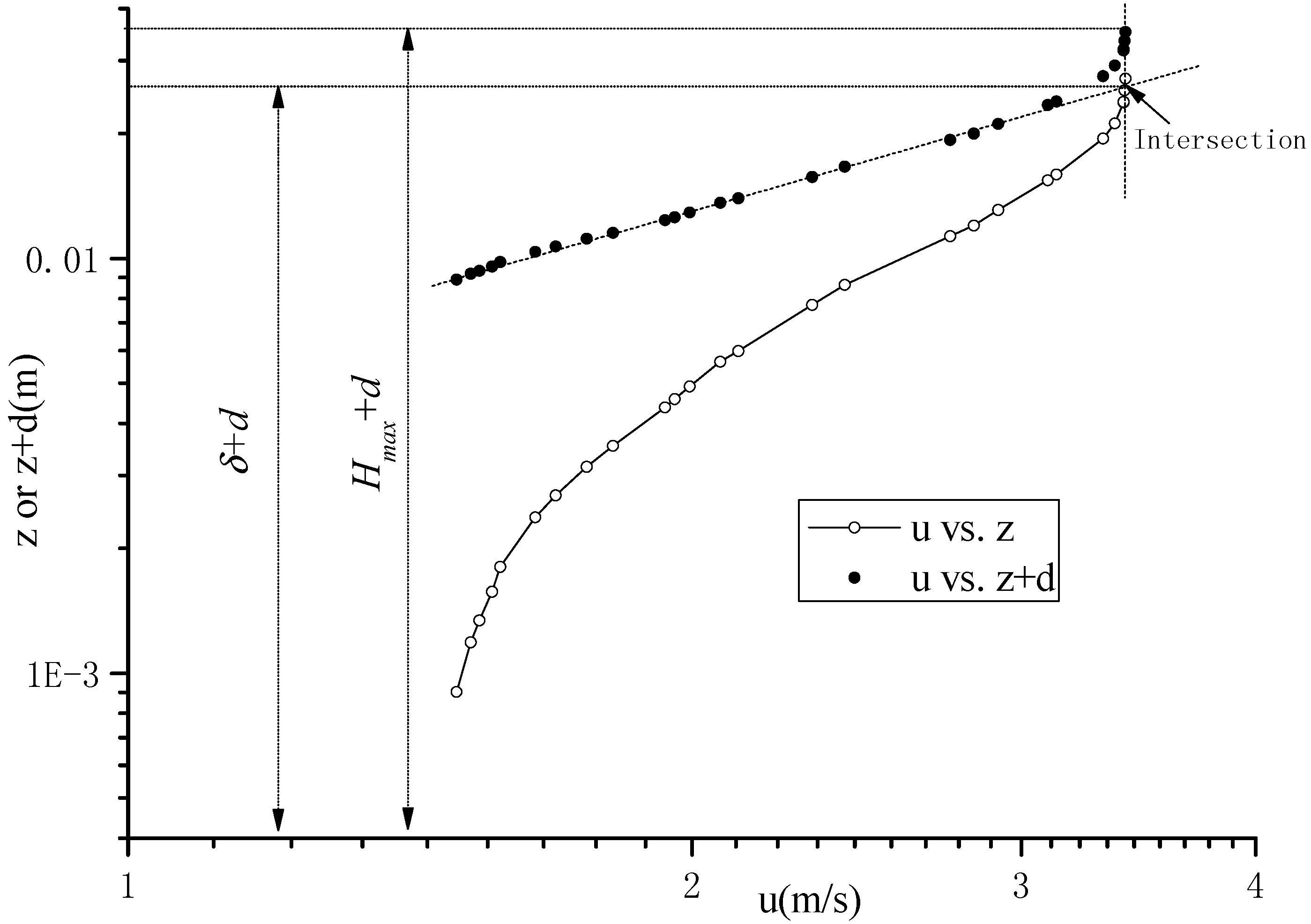
5.3. Application to Boundary Layer Development Length

According to the graphical method used by Bauer [64], a straight-line portion of a log-log plot of the velocity profile is extrapolated to its intersection with the line u = U. The value of z at this intersection is taken to be the value of turbulence boundary layer thickness, δ. Due to the effects of steps in the spillway, as illustrated in Figure 13, the log(u)–log(z) plot of the velocity profile is not a straight-line. Considering the displacement height d, a straight-line portion of a log(u)–log(z + d) plot, also shown in Figure 13, is extrapolated to its intersection with the line u = U. Theoretically, the value of z corresponding to the intersection is nearly equal to the flow depth at the maximum of velocity, U, where the corresponding water depth is defined by Hmax.
Figure 13. Schematic of the turbulence boundary layer thickness at the inception point.
Water 06 03888 g013
With skimming flow, there may occur air entrainment over a stepped spillway at a certain flow rate, such as the cases of 1, 5, 6, 7, 17 and 18 in Table 2. Following the increasing flow rates and the water depth increasing, the inception point of air entrainment may move downstream, there may be no air entrainment over stepped spillway, such as the cases of 2–4 and 8–16 in Table 2. To make the air entrainment occurrence at larger flow discharge, the length of stepped spillway need to be enlarged on the premise of sufficient building space. To track the inception point of air entrainment over stepped spillways in the paper, the length of numerical physical spillways were enlarged based on the original length of experimental spillways in the cases of 2–4 and 8–16.
Keller et al. [65] indicated that there may be three flow regions over a self-aerated spillway, one is the non-aerated region, where the turbulence boundary layer has not reached the water surface, one is aerating developing region, where the phenomena of aeration is developing, but the longitudinal profile of air void fraction keeps unstable along the spillway, another one is the aerating developed region, where the longitudinal profile of air void fraction keeps stable along the spillway.
In order to show the physical process of air entrainment and the detailed time history of air bubbles penetration over a stepped spillway clearly, Figure 14 gives the numerical void fraction of water under stable condition of Run No. 17. Also the part of numerical flow streamlines from second to fourth steps at Run No. 17 was also presented in the Figure 15.
Figure 14. Numerical void fraction of water on different instant at Run No. 17.
Water 06 03888 g014
Figure 15. Part of numerical flow streamlines from second to fourth steps at Run No. 17.
Water 06 03888 g015
Seen from the Figure 14 and Figure 15, first the water flowed down the stepped face as a coherent stream, skimming over the steps and cushioned by the re-circulating fluid trapped between them. The external edges of the steps formed a pseudo-bottom over which the skimming flow. Beneath this, re-circulating vortices formed and were sustained through the transmission of shear stress from the water flowing past the edge of the steps. The flow was transparent and no air entrainment took place from the crest to the step No. 4. This was the region of non-aeration. After step No. 4, the flow was characterized by air entrainment, where was the inception point of air entrainment and the turbulence boundary layer was reached at the water surface. At each step, a stable vortex developed and a continuous exchange of flow between top layer and vortices formed on the steps. The flow rotated in the vortex for a brief period and then returned to the main flow to proceed on down the spillway face. Similarly, air bubbles penetrated and rotated with the vortex flow, this was the region of developing aerated flow. Compared with the experimental boundary layer development length Li-exp, the numerical boundary layer development length Li-CFD was nearly equal to the Li-exp. Downstream of the inception point, the quantity air entrained increases, until the developed aeration region is reached.
Figure 16 shows the numerical contour maps of mean flow velocity u between the crest and the fifth step. Seen from Figure 15 and Figure 16, the closed velocity contour lines exist in the concave region of the steps, which indicates that there are vortices generated as the main means of energy dissipation on the stepped spillway. At the same time, it is observed that the mean flow velocities increase along the main flow direction. The velocity contour lines are from dense to sparse and the variation of flow velocities is from intense to gentle along the normal direction of pseudo-bottom. The maximum velocity U of each velocity profile along the normal direction of pseudo-bottom from the crest to downstream in Figure 16 has been reached under a certain depth below the water surface, until the location of measured air entrainment inception point, where the maximum of velocity U has been reached near the water surface and the turbulence boundary layer reached at the water surface.
Figure 16. Numerical contour map of mean flow velocity u at Run No. 17.
Water 06 03888 g016
According to the observed distance Li-exp from the crest to the inception point of air entrainment in the six experimental cases, the corresponding δ and Hmax at the inception point of air entrainment are achieved. Then the ratio (δ + d)/(Hmax + d) is calculated and between 0.72 and 0.79, for a median of 0.75, as shown in Table 3. Thus, as long as the ratio of (δ + d) and (Hmax + d) is roughly equal to 0.75, the air inception will occur and the boundary layer length Li will be achieved. So the Li-CFD of the other 12 numerical runs was calculated, as shown in Table 3. In all cases, the corresponding ratio is between 0.72 and 0.79.
Table 3. Summary of the information of velocity profiles at inception point.
Run No.d (m)δ (m)Hmax (m)Li-exp (m)Li-CFD (m)(δ + d)/(Hmax + d)
10.0080.01730.0270.600.660.72
50.0080.01070.0180.440.440.72
60.0100.04030.0573.443.440.75
70.0100.07130.0994.384.280.75
170.0230.04210.0601.351.350.78
180.0140.04030.0552.022.020.79
20.0100.01770.025-0.790.79
30.0050.01730.026-0.730.72
40.0120.02030.029-0.920.79
80.0100.1180.155-5.470.78
90.0100.1520.211-7.900.73
100.0200.1530.203-6.580.78
110.0150.1420.19-5.120.77
120.0090.1180.151-8.420.79
130.0090.1040.142-8.680.75
140.0090.1120.145-8.650.79
150.0090.12200.162-10.89 0.77
160.0100.12720.168-12.53 0.77
Taking into account the channel slope, θ, Froude surface roughness, F* and the surface roughness, ks, some relationships for determining the distance between the stepped spillway crest and the inception point were proposed by Chanson [66] (Equation (12)).
L i = 9.719   ( sin θ ) 0.08 ( F * ) 0.713   k s
The relationship proposed by Chanson [66] was then enhanced by Hunt and Kadavy [67] for flat-sloped stepped spillways
L i = 6.1   ( sin θ ) 0.08 ( F * ) 0.86   k s
The two relationships are applicable for the stepped spillways of F* less than 100. Then Hunt and Kadavy [68] proposed another relationship for broad-crested stepped spillways of 28 < F* < 100.
L i = 7.48   ( F * ) 0.78   k s
Table 4 summarizes the distance, Li simulated by numerical experiments, with regards to unit discharge, q, spillway slope, θ, surface roughness, ks and Froude surface roughness, F*. Also, the predicted Li calculated by Equations (12)–(14) from Chanson [66] and Hunt and Kadavy [67,68] are summarized in Table 4, respectively. The slope of spillways for numerical experiments ranges from 8.7° to 53.2°, which shows the numerical experiments include not only steep chute (θ ≥ 22°), but also flat-sloped spillways (θ ≤ 22°), and the corresponding F* ranges from 3.4 to 158.5. None of the Equations (12)–(14) seem to be accurate when the inception length is less than 1 m, but the authors probably were not emphasizing that region. At larger Li, all of the equations seem to function acceptably.
Table 4. Summary of unit discharge, Froude surface roughness and the distance calculated by Equations (12)–(14) and numerical experiments.
Run No.ksqθF*Li (m)Li (m)Li(m)Li-CFD
(cm)(m2/s)Equation (12)Equation (13)Equation (14)(m)
13.6000.153.25.21.120.890.980.66
24.4800.141.74.11.160.901.010.79
32.5000.133.710.81.271.131.200.73
44.9900.133.73.81.210.921.070.92
53.6000.0753.23.50.840.630.720.44
63.6900.2814.025.63.233.273.463.44
73.6900.4214.038.44.324.634.754.28
83.6870.6214.056.85.706.486.445.47
93.6870.8214.075.16.968.248.017.90
107.3730.8214.026.56.636.747.126.58
116.7980.8226.622.15.635.575.685.12
123.2471.2421.9110.78.3610.499.558.42
133.2471.2421.9110.78.3610.499.558.68
143.2471.2421.9110.78.3610.499.558.65
153.3801.2414.3128.09.3411.9711.1210.89
163.4491.248.7158.510.6814.1213.4012.53
179.2850.1821.83.41.981.491.791.35
185.0000.1521.86.91.781.481.712.02
Figure 17 provides direct comparison of the Li calculated by numerical experiments and Equations (12)–(14). When the F* is less than 32, the difference between the Li by the CFD, Chanson [66] and Hunt and Kadavy [67,68] are small. With the continuous increasing of F*, the errors between the Li calculated by numerical experiments and Equations (12) and (13) are larger, however, the values of Li calculated by numerical experiments are closer to the values calculated by Equation (14). The standard error of Equations (12)–(14) applied to the 18 numerical runs is 0.70, 0.76 and 0.38, respectively. All of the equations seem to be equivalent below F* = 32, but above F* = 64, Equation (14) by Hunt and Kadavy [68] is superior.
Figure 17. Normalized Li versus Froude surface roughness, F*.
Water 06 03888 g017

6. Conclusions

The length down crest to the air inception point in skimming flow over stepped spillway, is an important variable for many aspects of spillway design. It is dependent upon parameters of the velocity profile, such as dynamic roughness, displacement height and friction velocity. According to the numerical simulation results, the characterization relations for the three velocity profile parameters and finally the boundary layer development length for stepped spillways were developed. The conclusions are as follows:
(1)
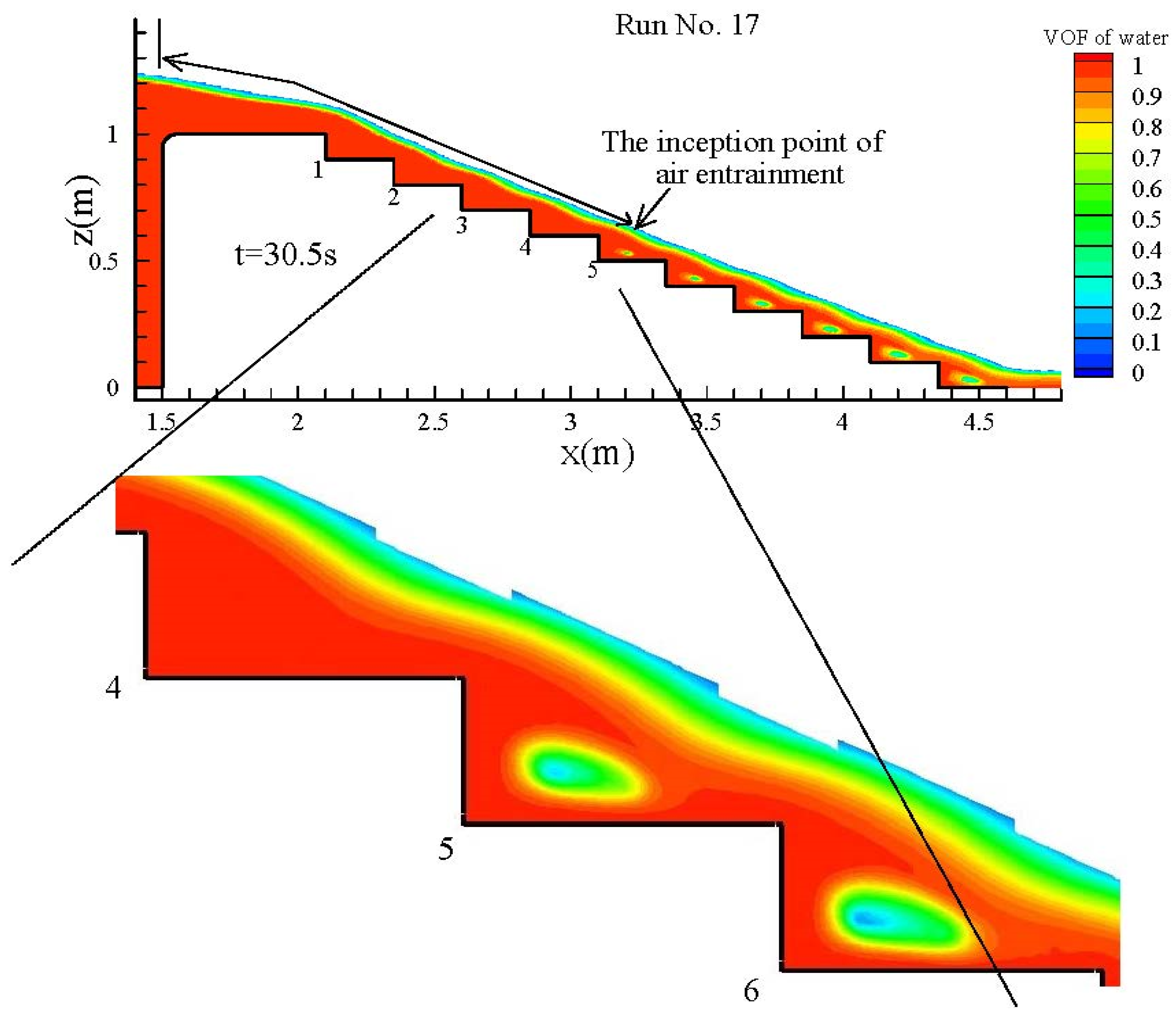
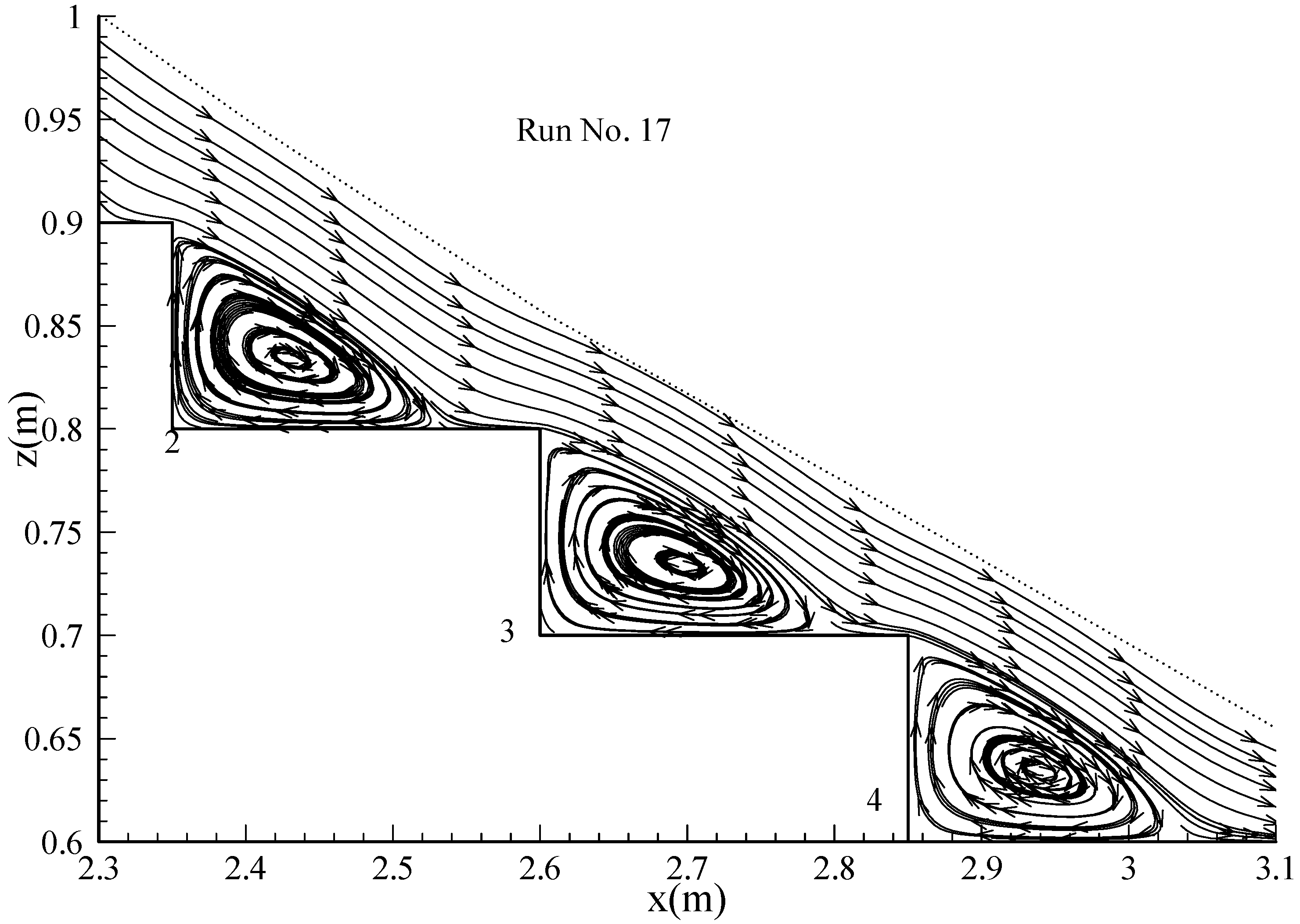
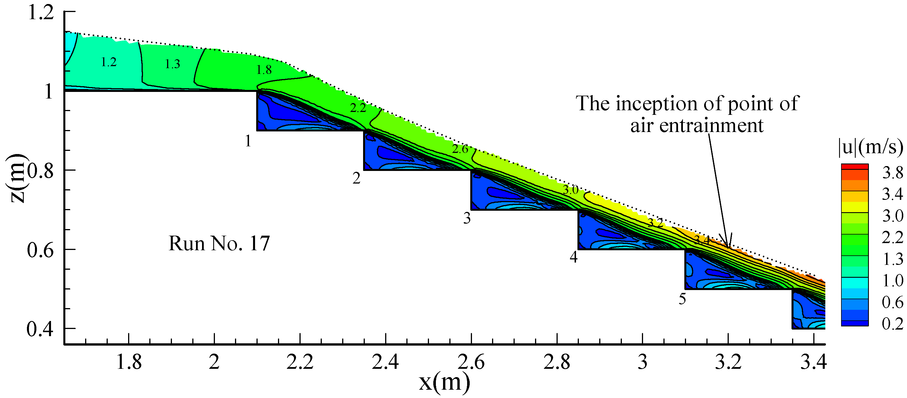
After validation with experimental data, numerical models and methods were used to simulate flow fields in the nonaerated skimming flow zones on stepped spillways. A two dimensional simulation was successful in simulating velocity profiles on stepped spillways.
(2)
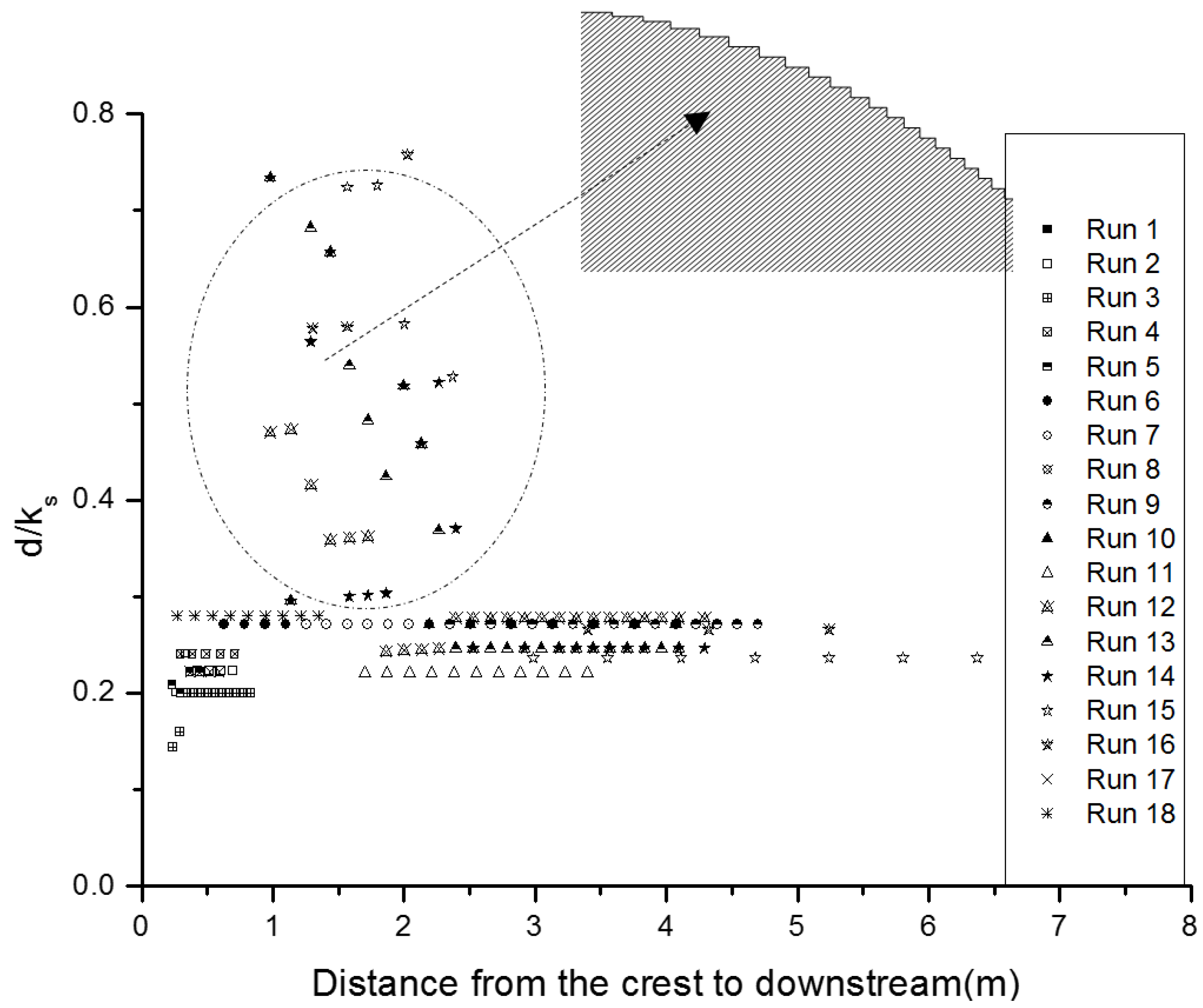
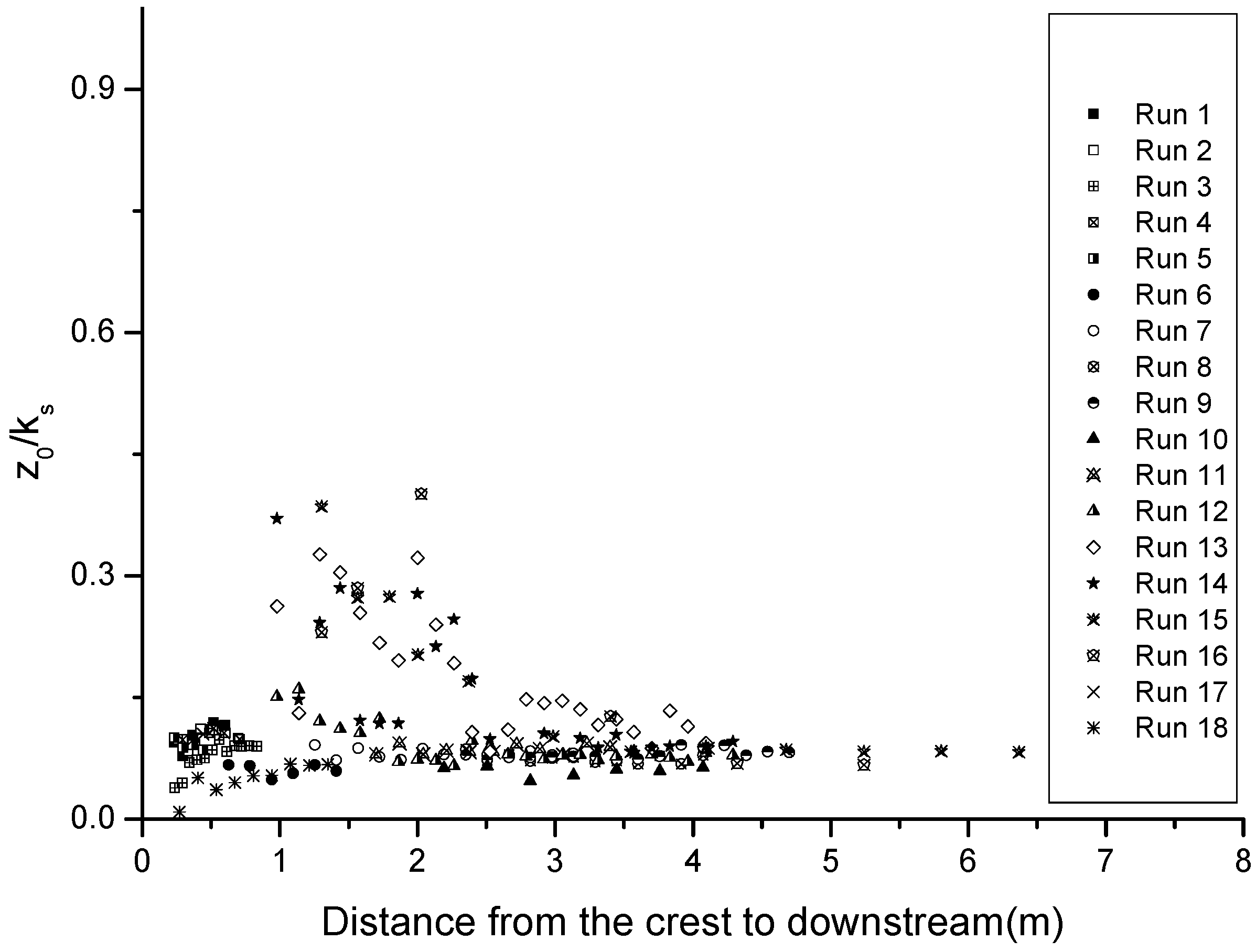
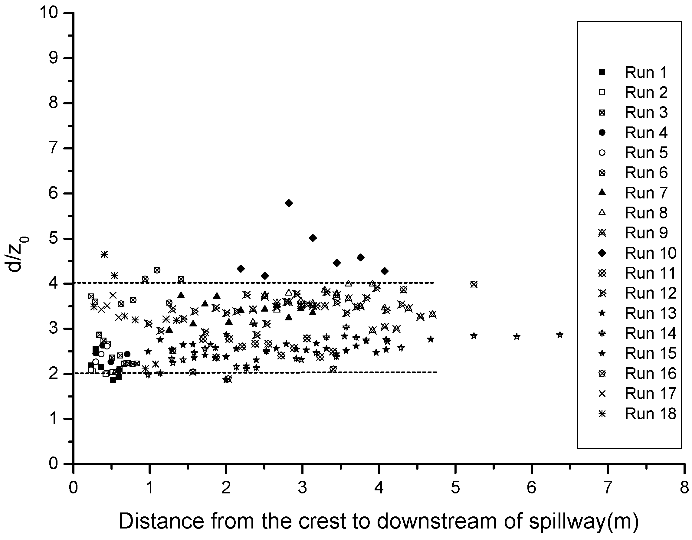
In many different step geometries and flow conditions, fixing the origin of vertical coordinate at the tip of the steps, the expressions of d/ks in the range of 0.22 to 0.27, z0/ks in the range of 0.06 to 0.1 and d/z0 from 2.2 to 4 give a good estimate along with the distance down the stepped spillways. It is a precondition that the rough stepped surfaces have a similar density of steps elements, since Figure 9 and Figure 10 illustrate that d and z0 may be strongly dependent on the density of roughness elements.
(3)
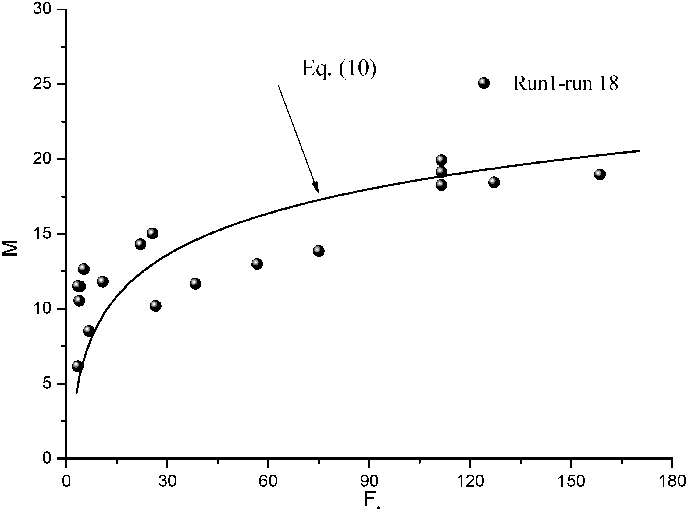
Equation (10) indicates that hydraulic roughness z0 is proportional to shear stress and the hydraulic roughness Froude number F*, defined in terms of the roughness height ks.
(4)
The turbulent boundary layer is seen at the water surface when the Bauer-defined boundary layer thickness is between 0.72 and 0.79 of the flow depth.
(5)
The length down the spillway to the inception of air entrainment is best predicted by Equation (13), developed by Hunt and Kadavy [68], especially when the surface roughness F* is equivalent above 64. However, the definition of inception point location in this paper is that the visual observation of the cross section where there is a continuous presence of air within the flow at the sidewalls or within the step cavities, and this conclusion was achieved based on the numerical simulation results under 18 different hydraulic conditions. Further research should expand the range of conditions for the application of these equations.

Acknowledgments

The study was undertaken while the first writer was a visiting scholar at the University of Minnesota. The first writer thanks the financial support of the China Scholarship Council (CSC), the National Natural Science Founding of China (Grant No. 50979118) and the University of Minnesota Joseph T. and Rose S. Ling Professorship fund.

Author Contributions

The idea of this study, literature research, simulations, figures, and preparation the every draft of the article were undertaken by Xiangju Cheng under the supervision of John S. Gulliver. Dantong Zhu made the contributions on doing graphics.

Conflicts of Interest

The authors declare no conflict of interest.

References

  1. Meireles, I.; Renna, F.; Matos, J.; Bombardelli, F. Skimming, nonaerated flow on stepped spillways over roller compacted concrete dams. J. Hydraul. Eng. 2012, 138, 870–877. [Google Scholar] [CrossRef]
  2. Chamani, M.R.; Rajaratnam, N. Jet flow on stepped spillways. J. Hydraul. Eng. 1994, 120, 254–259. [Google Scholar] [CrossRef]
  3. Chamani, M.R.; Rajaratnam, N. Characteristics of skimming flow over stepped spillways. J. Hydraul. Eng. 1999, 125, 361–368. [Google Scholar] [CrossRef]
  4. Chanson, H. Stepped spillway flows and air entrainment. Can. J. Civil Eng. 1993, 20, 422–435. [Google Scholar] [CrossRef]
  5. Chanson, H. Experimental investigations of air entrainment in transition and skimming flows down a stepped chute. Can. J. Civ. Eng. 2002, 29, 145–156. [Google Scholar] [CrossRef]
  6. Cheng, X.J.; Chen, Y.C.; Luo, L. Numerical simulation of air-water two-phase flow over stepped spillways. Sci. China Ser. E Technol. Sci. 2006, 49, 674–684. [Google Scholar] [CrossRef]
  7. Cheng, X.J.; Chen, X.W. Numerical simulation of dissolved oxygen concentration in water flow over stepped spillways. Water Environ. Res. 2013, 85, 434–446. [Google Scholar] [CrossRef] [PubMed]
  8. Meireles, I.; Matos, J. Skimming flow in the nonaerated region of stepped spillways over embankment dams. J. Hydraul. Eng. 2009, 135, 685–689. [Google Scholar] [CrossRef]
  9. Chanson, H. Hydraulics of skimming flows on stepped chutes: The effects of inflow conditions. J. Hydraul. Res. 2006, 44, 51–60. [Google Scholar] [CrossRef] [Green Version]
  10. Bung, D.B. Developing flow in skimming flow regime on embankment stepped spillways. J. Hydraul. Res. 2011, 49, 639–648. [Google Scholar] [CrossRef]
  11. Amador, A.; Sanchez-Juny, M.; Dolz, J. Characterization of the nonaerated flow region in a stepped spillway by PIV. J. Fluids Eng. 2006, 128, 1266–1273. [Google Scholar] [CrossRef]
  12. Smart, G.M. Turbulent velocity profiles and boundary shear in gravel bed rivers. J. Hydraul. Eng. 1999, 125, 106–116. [Google Scholar] [CrossRef]
  13. Franca, M.J.; Ferreira, R.M.; Lemmin, U. Parameterization of the logarithmic layer of double-averaged streamwise velocity profiles in gravel-bed river flows. Adv. Water Resour. 2008, 31, 915–925. [Google Scholar] [CrossRef]
  14. Wang, J.J.; Dong, Z.N. Open-channel turbulent flow over non-uniform gravel beds. Appl. Sci. Res. 1996, 56, 243–254. [Google Scholar] [CrossRef]
  15. Perry, A.E.; Schofield, W.H.; Joubert, P.N. Rough wall turbulent boundary layers. J. Fluid Mech. 1969, 37, 383–413. [Google Scholar] [CrossRef]
  16. Millikan, C.B. A critical discussion of turbulent flow in channels and circular tubes. In Proceedings of the Fifth International Congress for Applied Mechanics, Cambridge, MA, USA, 12–16 September 1938; Den Hartog, J.P., Peter, H., Eds.; Wiley: New York, NY, USA, 1938; pp. 386–392. [Google Scholar]
  17. Jackson, P.S. On the displacement height in the logarithmic velocity profile. J. Fluid Mech. 1981, 111, 15–25. [Google Scholar] [CrossRef]
  18. Bridge, J.S.; Jarvis, J. The dynamics of a river bend: A study in flow and sedimentary processes. Sedimentology 1982, 29, 499–541. [Google Scholar] [CrossRef]
  19. Nezu, I.; Nakagawa, H. Turbulence in Open-Channel Flows; Brookfiel, Balkema: Rotterdam, The Netherlands, 1993. [Google Scholar]
  20. Ferguson, R.I.; Prestegaard, K.L.; Ashworth, P.J. Influence of sand on hydraulics and gravel transport in a braided gravel bed river. Water Resour. Res. 1989, 5, 635–643. [Google Scholar] [CrossRef]
  21. Stephan, U.; Gutknecht, D. Hydraulic resistance of submerged flexible vegetation. J. Hydrol. 2002, 269, 27–43. [Google Scholar] [CrossRef]
  22. Klopstra, D.; Barneveld, H.J.; van Noortwijk, J.M.V.; van Velzen, E.H. Analytical model for hydraulic roughness of submerged vegetation. In Managing Water: Coping with Scarcity and Abundance, Proceedings of the 27th Congress of the International Association for Hydraulic Research, San Francisco, CA, USA, 10–15 August 1997.
  23. Bandyopadhyay, P.R. Rough-wall turbulent boundary layers in the transition regime. J. Fluid Mech. 1987, 180, 231–266. [Google Scholar] [CrossRef]
  24. Lo, K.L. On the determination of zero-plane displacement and roughness length for flow over forest canopies. Bound. Layer Meteorol. 1990, 51, 255–268. [Google Scholar] [CrossRef]
  25. Molion, L.C.B.; Moore, C.J. Estimating the zero-plane displacement for tall vegetation using a mass conservation method. Bound. Layer Meteorol. 1983, 26, 115–125. [Google Scholar] [CrossRef]
  26. Bergeron, N.E.; Abrahams, A.D. Estimating shear velocity and roughness length from velocity profiles. Water Resour. Res. 1992, 28, 2155–2158. [Google Scholar] [CrossRef]
  27. Yu, G.L.; Tan, S. Errors in the bed shear stress as estimated from vertical velocity profile. J. Irrig. Drain. Eng. 2006, 132, 490–497. [Google Scholar] [CrossRef]
  28. Bergstrom, D.J.; Kotey, N.A.; Tachie, M.F. The effects of surface roughness on the mean velocity profile in a turbulent boundary layer. J. Fluids Eng. 2002, 124, 664–670. [Google Scholar] [CrossRef]
  29. Avelino, M.R.; Freire, A.P.S. On the displacement in origin for turbulent boundary layers subjected to sudden changes in wall temperature and roughness. Int. J. Heat Mass Trans. 2002, 45, 3143–3153. [Google Scholar] [CrossRef]
  30. Chanson, H. The Hydraulics of Stepped Chutes and Spillways; Balkema Publisher: Lisse, The Netherlands, 2002. [Google Scholar]
  31. Boes, R.M.; Hager, W.H. Two-phase flow characteristics of stepped spillways. J. Hydraul. Eng. 2003, 129, 661–670. [Google Scholar] [CrossRef]
  32. Boes, R.M.; Hager, W.H. Hydraulic design of stepped spillways. J. Hydraul. Eng. 2003, 129, 671–679. [Google Scholar] [CrossRef]
  33. Chanson, H.; Toombes, L. Strong interactions between free-surface aeration and turbulence in an open channel flow. Exp. Therm. Fluid Sci. 2003, 27, 525–535. [Google Scholar] [CrossRef]
  34. Ohtsu, I.; Yasuda, Y.; Takahashi, M. Flow characteristics of skimming flows in stepped channels. J. Hydraul. Eng. 2004, 130, 860–869. [Google Scholar] [CrossRef]
  35. Gonzalez, C.A.; Takahashi, M.; Chanson, H. An experimental study of effects of step roughness in skimming flows on stepped chutes. J. Hydraul. Res. 2008, 46, 24–35. [Google Scholar] [CrossRef]
  36. Bombardelli, F.A.; Meireles, I.; Matos, J. Laboratory measurements and multi-block numerical simulations of the mean flow and turbulence in the non-aerated skimming flow region of steep stepped spillways. Environ. Fluid Mech. 2011, 11, 263–288. [Google Scholar] [CrossRef]
  37. Tabbara, M.; Chatila, J.; Awwad, R. Computational simulation of flow over stepped spillways. Comput. Struct. 2005, 83, 2215–2224. [Google Scholar] [CrossRef]
  38. Carvalho, R.F.; Martins, R. Stepped spillway with hydraulic jumps: Application of a numerical model to a scale model of a conceptual prototype. J. Hydraul. Eng. 2009, 135, 615–619. [Google Scholar] [CrossRef]
  39. Musavi-Jahromi, H.; Bina, M.; Salmasi, F. Physical and numerical modeling of the Nappe flow in the stepped spillways. J. Appl. Sci. 2008, 8, 1720–1725. [Google Scholar] [CrossRef]
  40. Tongkratoke, A.; Chinnarasri, C.; Pornprommin, A.; Dechaumphai, P.; Juntasaro, V. Non-linear turbulence models for multiphase recirculating free-surface flow over stepped spillways. Int. J. Comput. Fluid Dyn. 2009, 23, 401–409. [Google Scholar] [CrossRef]
  41. Chen, Q. Turbulence Numerical Simulation and Model Test of the Stepped Spillway Overflow. Ph.D. Thesis, Sichuan University, Chengdu, China, 2001. [Google Scholar]
  42. Cheng, X.J.; Luo, L.; Zhao, W.Q.; Li, R. Two-phase flow simulation of aeration on stepped spillway. Prog. Nat. Sci. 2004, 14, 626–630. [Google Scholar] [CrossRef]
  43. Qian, Z.D.; Hu, X.Q.; Huai, W.X.; Amador, A. Numerical simulation and analysis of water flow over stepped spillway. Sci. China Ser. E Technol. Sci. 2009, 52, 1958–1965. [Google Scholar] [CrossRef]
  44. André, S.; Dewals, B.J.; Pirotton, M.; Schleiss, A. Quasi 2D-numerical model of aerated flow over stepped chutes. In Proceedings of the 30th International Association for Hydro-Environment Engineering and Research (IAHR) Congress, Thessaloniki, Greece, 24–29 August 2003; Ganoulis, J., Prinos, P., Eds.; IAHR: Thessaloniki, Greece; Volume D, pp. 671–678.
  45. Dewals, B.J.; André, S.; Schleiss, A.; Pirotton, M. Validation of a quasi-2D model for aerated flows over stepped spillways for mild and steep slopes. In Proceedings of the 6th International Conference of Hydroinformatics, Singapore, 21–24 June 2004; pp. 63–70.
  46. Fluent User’s Guide. Fluent Incorporated: Lebanon, NH, USA, 2006. Available online: http://www.ansys.com/Products/Simulation+Technology/Fluid+Dynamics/Fluid+Dynamics+Products/ANSYS+Fluent (accessed on 20 September 2014).
  47. Bijan, D. Experimental study and 3D numerical simulations for a free-overflow spillway. J. Hydraul. Eng. 2006, 132, 899–907. [Google Scholar] [CrossRef]
  48. Lueker, M.L.; Mohseni, O.; Gulliver, J.S.; Schulz, H.; Christopher, R.A. The Physical Model Study of the Folsom Dam Auxiliary Spillway System; Project Report 511; University of Minnesota, St. Anthony Falls Laboratory: Minneapolis, MI, USA, 2008. [Google Scholar]
  49. Hunt, S.L.; Kadavy, K.C. Velocities and energy dissipation on a flat-sloped stepped spillway. In Proceedings of the 2008 American Society of Agricultural and Biological Engineers (ASABE) Annual International Meeting, Providence, RI, USA, 29 June–2 July 2008.
  50. Kiya, M.; Sasaki, K.; Arie, M. Discrete-vortex simulation of a turbulent separation bubble. J. Fluid Mech. 1982, 120, 219–244. [Google Scholar] [CrossRef]
  51. Carosi, G.; Chanson, H. Air-Water Time and Length Scales in Skimming Flows on a Stepped Spillway, Application to the Spray Characterization; Report CH 59/06; The University of Queensland: Brisbane, Australia, 2006. [Google Scholar]
  52. Felder, S.; Chanson, H. Turbulence and Turbulent Length and Time Scales in Skimming Flows on a Stepped Spillway, Dynamic Similarity, Physical Modeling and Scale Effects; Report CH64/07; The University of Queensland: Brisbane, Australia, 2007. [Google Scholar]
  53. Charnock, H. Wind stress on a water surface. Q. J. R. Meteorol. Soc. 1955, 81, 639–640. [Google Scholar] [CrossRef]
  54. Counihan, J. Wind tunnel determination of the roughness length as a function of the fetch and the roughness density of three dimensional elements. Atmos. Environ. 1971, 5, 637–642. [Google Scholar] [CrossRef]
  55. Lee, B.E.; Soliman, B.F. An investigation of the forces on three-dimensional bluff bodies in rough wall turbulent boundary layers. Trans. ASME J. Fluids Eng. 1977, 99, 503–510. [Google Scholar] [CrossRef]
  56. O’Loughlin, E.M.; Annambhotla, V.S. Flow phenomena near rough boundaries. J. Hydraul. Res. 1969, 7, 231–250. [Google Scholar] [CrossRef]
  57. Blihco, R.G.; Partheniades, E. Turbulence characteristics in free surface flows over smooth and rough boundaries. J. Hydraul. Res. 1971, 9, 43–69. [Google Scholar] [CrossRef]
  58. Thom, A.S. Momentum absorption by vegetation. Q. J. Roy. Meteorol. Soc. 1971, 97, 414–428. [Google Scholar] [CrossRef]
  59. Nepf, H.M.; Vivoni, E.R. Flow structure in depth-limited, vegetated flow. J. Geophys. Res. 2000, 105, 28547–28557. [Google Scholar] [CrossRef]
  60. Whiting, P.J.; Dietrich, W.E. The roughness of alluvial surfaces and experimental examination of the influence of size heterogeneity and natural packing. EOS Trans. Am. Geophys. Union 1989, 70, 329. [Google Scholar]
  61. Brutsaert, W. Evaporation into the Atmosphere: Theory, History, and Applications; Kluwer Academic: Dordrecht, The Netherlands, 1982. [Google Scholar]
  62. Chamberlain, A.C. Roughness length of sea, sand, and snow. Bound. Layer Meteorol. 1983, 25, 405–409. [Google Scholar] [CrossRef]
  63. Keller, R.J.; Rastogi, A.K. Design chart for predicting critical point on spillways. J. Hydraul. Div. 1977, 103, 1417–1429. [Google Scholar]
  64. Bauer, W.J. Turbulent boundary layer on steep slopes. Trans. Am. Soc. Civ. Eng. 1954, 119, 1212–1233. [Google Scholar]
  65. Keller, R.J.; Lai, K.K.; Wood, I.R. Developing region in self aerating flows. Proc. ASCE J. Hyd. Div. 1974, 100, 553–568. [Google Scholar]
  66. Chanson, H. Hydraulics of skimming flows over stepped channels and spillways. J. Hydraul. Res. 1994, 32, 445–460. [Google Scholar] [CrossRef]
  67. Hunt, S.L.; Kadavy, K.C. Inception point relationship for flat-sloped stepped spillways. J. Hydraul. Eng. 2011, 137, 262–266. [Google Scholar] [CrossRef]
  68. Hunt, S.L.; Kadavy, K.C. Inception point for embankment dam stepped spillways. J. Hydraul. Eng. 2013, 139, 60–64. [Google Scholar] [CrossRef]

