MODIS Inundation Estimate Assimilation into Soil Moisture Accounting Hydrologic Model: A Case Study in Southeast Asia

Abstract

Flash Flood Guidance consists of indices that estimate the amount of rain of a certain duration that is needed over a given small basin in order to cause minor flooding. Backwater catchment inundation from swollen rivers or regional groundwater inputs are not significant over the spatial and temporal scales for the majority of upland flash flood prone basins, as such, these effects are not considered. However, some lowland areas and flat terrain near large rivers experience standing water long after local precipitation has ceased. NASA is producing an experimental product from the MODIS that detects standing water. These observations were assimilated into the hydrologic model in order to more accurately represent soil moisture conditions within basins, from sources of water from outside of the basin. Based on the upper soil water content, relations are used to derive an error estimate for the modeled soil saturation fraction; whereby, the soil saturation fraction model state can be updated given the availability of satellite observed inundation. Model error estimates were used in a Monte Carlo ensemble forecast of soil water and flash flood potential. Numerical experiments with six months of data (July 2011–December 2011) showed that MODIS inundation data, when assimilated to correct soil moisture estimates, increased the likelihood that bankfull flow would occur, over non-assimilated modeling, at catchment outlets for approximately 44% of basin-days during the study time period. While this is a much more realistic representation of conditions, no actual events occurred allowing for validation during the time period.

1. Introduction

The mapping of floods from space using orbital sensors has many applications toward the goal of reducing the detrimental effects of extreme flood events on society. Efforts to develop flood hazard maps for planning purposes, rapid-response flood mapping for disaster response activities, and the detection of new flood events and public warnings thereof are some of the applications of orbital detection systems [1,2,3,4]. Various other efforts and strategies to exploit the opportunities from these data sources evolved based on the spatial and temporal resolution of the orbital sensor and the goals and objectives of the various programs, including coastal storm surge [5], river flooding stage and discharge [6,7], land classification mapping [8], and the monitoring of suspended sediment concentrations [9], to name a few. The efforts elaborated herein represent a new strategy for the use of satellite derived inundation maps, by using the flood water boundary to represent the fractional inundation occurring in a given watershed, as a proxy for the upper zone soil moisture that can be assimilated into a hydrologic model.

The development of regional flash flood warning-response systems is a high priority due to the status of flash floods as the natural disaster with the highest mortality rate; more than 5000 deaths worldwide every year on average [10]. The goal of a flash flood guidance system is to produce estimates of impending flash flood threat for small basins in a region. The use of a continuous soil moisture accounting hydrologic model to estimate flash flood threat is developed by Carpenter et al. [11] and Georgakakos [12]. This modeling strategy uses a conservation of mass approach in a number of soil moisture reservoirs representing upper and lower zone soil moisture dynamics in each basin. To compute flash flood guidance it is necessary to estimate the soil water deficit for each small basin. When soil water storage reservoirs are filled for a small basin, under continuing rain, there is high potential for flash flood development.

In the typical implementation, the computational core at a regional center runs meso-scale meteorological models and high resolution hydrologic models for the region that produce various diagnostic indices and nowcasts/forecasts of precipitation, soil water deficit and flash flood potential for small streams on the basis of global meteorological model forecasts (ensemble forecasts in some cases), satellite estimates of precipitation with high resolution and short latency and real time operational raingauge and surface weather station reports. An example of these regional systems is described in Integrating Multiscale Observations of US Waters [13], whereby the basis of the first regional system implemented and operated since 2004 in Central America is discussed. System application is described most recently in Shamir et al. [14]. The systems support the elements identified in WMO [15] for effective flash flood prediction and warning.

Use of remotely sensed and on site data is made to produce estimates of mean areal precipitation (MAP) for each one of the small basins in the region. Existing and in progress implementations use (a) the global NOAA/NESDIS Hydroestimator rainfall (~4 km × 4 km half hourly values with latency of a few minutes up to half hour) (e.g., [16]) as the basic real time satellite rainfall product, (b) the CMORPH satellite rainfall (~8 km × 8 km half hourly values with 18 hour latency) (e.g., [17]) to update soil water deficit fields up to 18 hours from present and to provide bias estimates for the Hydroestimator in regions with no surface gauge information, and (c) real-time gauge rainfall reports to estimate bias and adjust the satellite rainfall products. The latter involves the use of adaptive Kalman Filtering that estimates the error variances for the bias and propagates it to the adjusted rainfall fields (e.g., [18,19]). Optimization of satellite derived rainfall estimates was refined for South Africa by de Coning [20]. The process of bias adjustment and blending of the satellite and gauge fields occurs every time the computational component runs (typically every 6 hours) and it involves a two-week window that ends at the current time.

Soil moisture is the principal state variable in estimating the rainfall-runoff relationship in a given catchment and the likelihood of flash flooding. Antecedent soil moisture conditions directly impact the ability of additional precipitation inputs to infiltrate, rather than becoming surface runoff. Factors that affect the soil moisture conditions, and thus the threat of flash flooding, include land use, vegetation, and infrastructure. In the operational flash flood guidance systems, the focus is on the water balance over the flash-flood prone small watersheds, rainfall-runoff relationships are driven solely by those processes (e.g., rainfall, snow melt, evapo-transpiration) that occur within each separate hydrologic basin. Downstream inundation effects or large scale groundwater effects are not significant for the majority of the upland flash flood prone basins; thus, these effects are not considered. However, some lowland areas and flat terrain near large rivers experience standing water long after local precipitation has ceased. This standing water may be the result of backwater effects from swollen rivers or elevated groundwater levels from upland source areas. Therefore, these outside sources of water may greatly impact the soil water deficit within a small flash flood prone basin. The NASA Office of Applied Science is producing an experimental product from the MODIS instrument on the Terra and Aqua satellites that detects standing water, beyond reference water, at a daily time interval and with a 250 m resolution. This work explores the potential utility of this product to adjust the soil water estimates of the operational systems for flash flood prone basins in low lying areas to improve local flash flood warnings.

2. Methods

The works presented herein documents a new method for the assimilation of NASA Global MODIS Flood Mapping products into the hydrologic soil water accounting models that support flash flood warning in small basins that tile a large region. Watershed basin boundaries in a lumped hydrologic model are determined based on elevation data and the approximate size of the desired basins. MODIS Real-time Flood Map 250 m resolution grids are overlaid on top of watershed boundaries. Mapping of pixels to watershed basins is done based on the location of pixel centroids. Thus, the flood water map observations undergo preprocessing to map the fractional area of inundation to each small catchment. The basin fractional inundation is then used to determine the modeled soil water deficit error. The error is then corrected using the fractional inundation observations.

Consider that small flash-flood prone catchment of area A. For this catchment, the soil water component of the flash flood guidance system provides estimates of upper (in the top 20–30 cm of soil depth) soil saturation ratio, w, at hourly or six-hourly intervals. Compared to the actual soil saturation ratio of the upper soil, w_a, the model estimate is considered to have an additive random error ζ:

w_a = w + ζ

(1)

This random error may have a non-zero mean and it is present in all the simulated values w in small catchments. Its probability distribution characterizes errors in simulated soil saturation fraction due to uncertainties in catchment precipitation and potential evapotranspiration. Error distribution is also due to uncertainties in the soil water models used for the particular catchment (due to both parametric and model-structure errors). These errors are only associated with the local catchment forcing and models. For catchments that in part of their area experience soil saturation influences from downstream large-river inundation or groundwater rise, it is necessary to define an additional random variable, v, to represent the error of the modeled soil saturation fraction (that in the flash flood guidance systems does not include these non-local effects).

Processing of real time satellite earth observations provides a daily estimate of fractional inundation (fraction of area, A, under water), which is denoted by f. Thus, the corrected upper soil saturation fraction for the basin, w’, for these cases is:

w’ = w + v

(2)

The aim of the formulation is to estimate w’ for times of significant flood inundation fractions, and to estimate its uncertainty.

The capacity of the upper soil zone to hold water (the product of the upper soil effective porosity and the upper soil zone depth) is denoted by U, and it represents the maximum volume of water the small basin upper soils can hold divided by the area of the basin. The total volume V of the upper soil water content can then be expressed as follows:

V = 1 f A U + w_a (1 − f) A U

(3)

and

V = (w + v) U A

(4)

where w_a is the actual saturation fraction of the upper soils in the portion of the area that is not inundated. Equation (2) is based on the reasonable assumption that if there is surface inundation, the upper soil zone (down to 20–30 cm) is saturated (saturation fraction = 1). Because of the equivalence of the volumes on the left hand side and the presence of a common factor involving the product of area (A) and upper soil water capacity (U), Equations (3) and (4) yield:

w’ = w + v = f + (1 − f) w_a

(5)

this equation connects the model-produced w and its uncertainty (in the form of an additive error term) with the satellite-based fractional inundation, f, through the unknown upper soil water saturation fraction, w_a, that actually exists in the portion of the area A without water inundation. It is noted that two limiting conditions arise for which additional information may be derived: (a) the case of zero inundation (f = 0), and (b) the case of full inundation (f = 1). In these two limiting cases the following apply:

w + v = w_a; f = 0

(6)

and

w + v = 1; f = 1

(7)

the first condition in Equation (6) represents the definition of the error term (v = w_a – w) for cases of no inundation and for which v = ζ, and the second condition in Equation (7) provides an estimate of the error in case of full inundation. Namely:

v = 1 − w; f = 1

(8)

thus, the error may be estimated from full inundation cases (or approximately full inundation cases) by developing the histogram of the estimates (1 − w). If a sufficient sample of inundation cases is available, then the mean or median and the standard deviation of the error may be derived. If a large enough sample of full inundation cases are available then quantiles of the error can also be derived.

It is noted that these error properties are associated with full inundation and not necessarily with cases having inundation substantially lower than 1. In addition, the error, v, is the result of both the small basin soil water model parametric and input errors (i.e., ζ), but it also may be related to external input not modeled (model structure error) such as exist during large river flooding with backwater effects on neighboring small tributary catchments. In the latter case, satellite data of inundation provides the only means of model correction.

Substituting w_a in Equation (5) from Equation (1) one may derive for all inundation fractions:

w’ = w + v = f + (1 − f) (w + ζ)

(9)

which yields the following relationship between v and ζ:

v = f (1 − w) + (1 − f)ζ

(10)

the relationship v versus ζ is linear, thus if one has a normal distribution so does the other. Knowing the mean and variance of v yields the mean and variance of ζ and vice versa. Uncertainty in f may also be taken into consideration but for this development and as a first approach we make the reasonable assumption that the error in f (after quality control) is much smaller than the error in w, and therefore f may be considered to be non-random. The resultant relationships are given below:

m_v = f (1 − w) + (1 − f)m_ζ

(11)

VAR(v) = (1 − f)² VAR(ζ)

(12)

where m_v and VAR(v) represent the mean and variance of v, and m_ζ and VAR(ζ) represent the mean and variance of ζ.

As mentioned earlier, for near full inundation (f = 1) one may define the distributional characteristics of v (see Equation (8) and associated discussion). Using Equations (11) and (12) one may also define the two moments of the distribution of ζ for these full inundation conditions (i.e., f > f_T where f_T is close to 1). The corrected model saturation fraction for the upper soil in the catchment, w’, may then be obtained from Equation (9), w’ = f + (1 − f) (w + ζ), and, together with the error properties of ζ, may be used in a Monte-Carlo-based ensemble simulation of corrected values.

A normalized measure of the correction in model upper soil saturation fraction (B_F) may be defined as follows:

B_F = (w’ – w)/w

(13)

and for the case under examination (f > f_T),

B_F = f (1 − w)/w + (1 − f) (ζ/w);  f > f_T

(14)

this may be used with a description of the statistical properties of the error ζ estimated for near full inundation conditions as discussed above to derive the statistical properties of the normalized correction B_F for a given set of values of f and w. For normally distributed ζ the distribution of B_F is also normal.

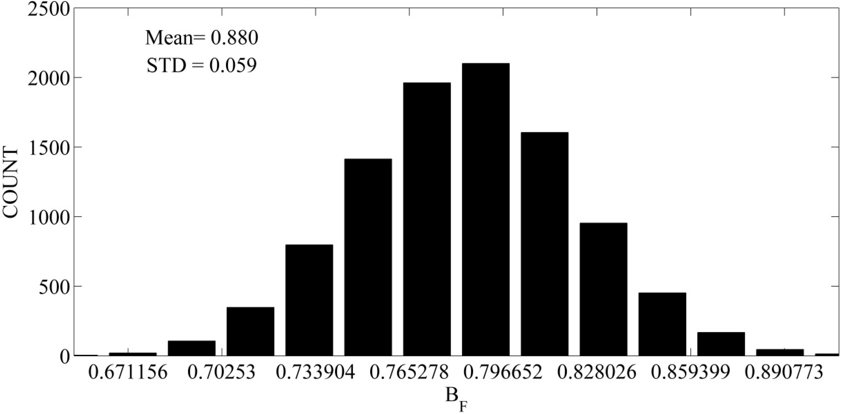
Figure 1 exemplifies the distribution of the B_F values for the case of f = 0.85, w = 0.5, and for ζ normally distributed with mean value of 0.1 and standard deviation equal to 0.2 (substantial uncertainty is assumed). A total number of 10,000 samples were used to create the histogram shown.

Figure 1. Histogram of B_F for w = 0.5, f = 0.85, and v~N(0.1,0.2).

Figure 1. Histogram of B_F for w = 0.5, f = 0.85, and v~N(0.1,0.2).

The results show a normal distribution of the fractional normalized correction (see Equation (13)) but with a mean of about 0.88 and a standard deviation of about 0.06. The coefficient of variation (0.06/0.88) of the normalized correction, B_F, is significantly lower than that of the model error ζ (0.2/0.1) for the given values of f and w. That is, for high fractional inundation values (in this case 0.85) even high model error uncertainty results in low uncertainty in the corrected soil saturation fraction.

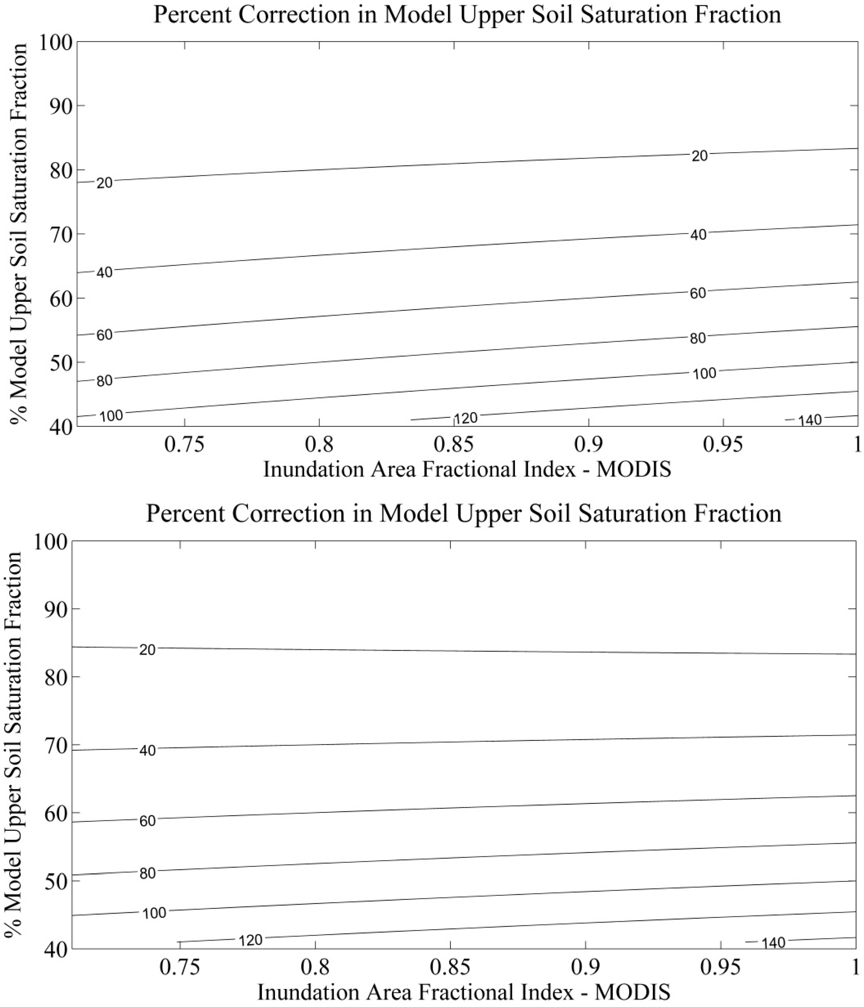
Taking the expected value of Equation (14) for the case of zero mean ζ yields the result:

B_F = f (1 − w)/w;  f > f_T

(15)

which is depicted in the upper panel of Figure 2 for a range of values of w and f. The lower panel of Figure 2 corresponds to a mean value of ζ that is equal to 0.2 (positive bias of 20%).

Figure 2. Mean B_F as function of f (fraction) and w (in %) for Mean(v) = 0 (upper panel) and Mean(v) = 0.2 (lower panel).

Figure 2. Mean B_F as function of f (fraction) and w (in %) for Mean(v) = 0 (upper panel) and Mean(v) = 0.2 (lower panel).

The results in Figure 2 show that for the range of near full inundation values of f, the percent normalized correction factor B_F exhibits much lower sensitivity to the value of f than to the value of w. The addition of a bias in the model estimates (mean value of v is equal to 0.2 or 20%) further reduces the sensitivity of the normalized correction factor to the value of f (for f > 0.70) and especially for values of w greater than 70%.

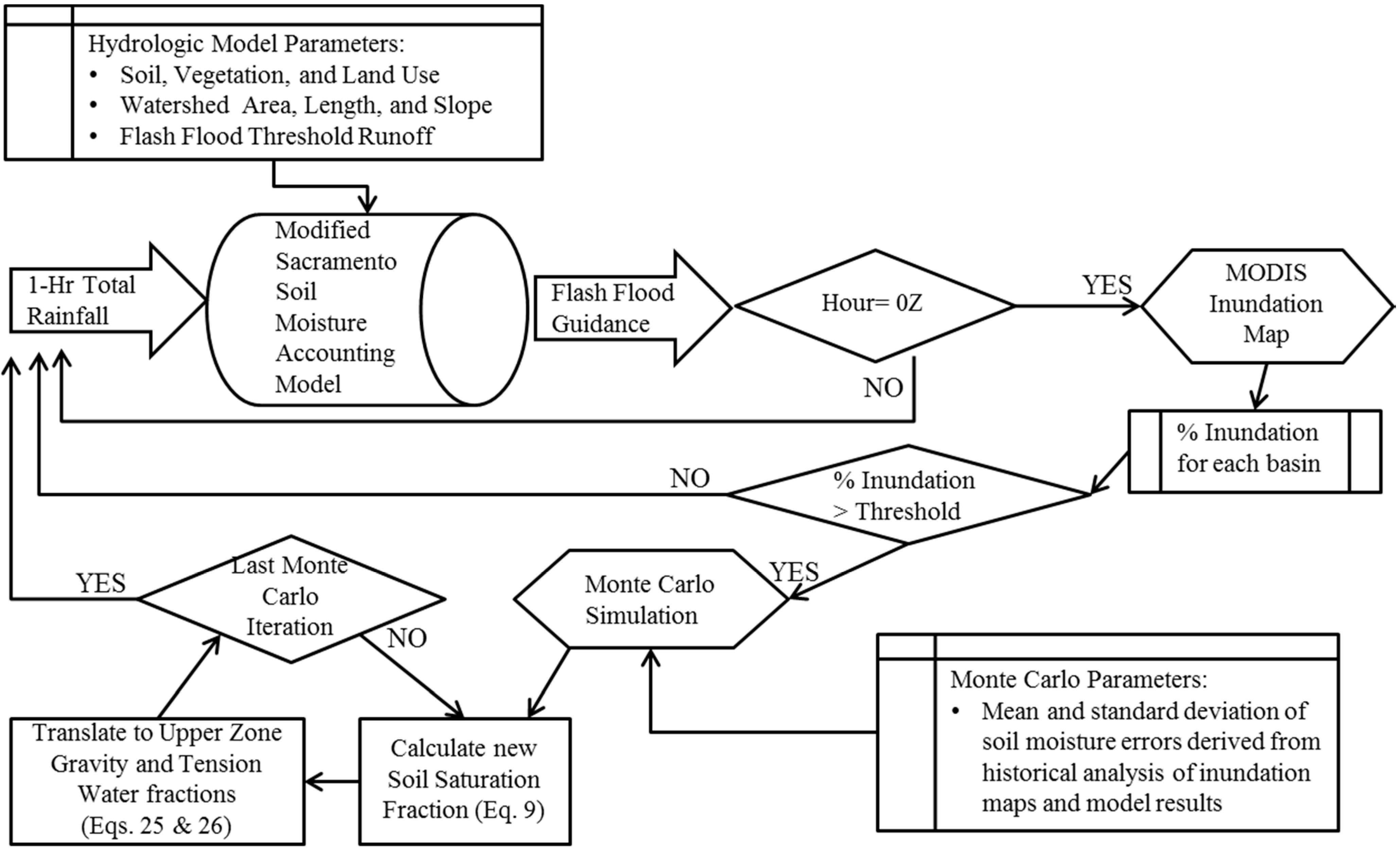
The previous discussion supports the following methodology for incorporating satellite-based inundation fraction values (f) into the flash flood guidance system soil water accounting model for values of f > f_T (Figure 3):

Figure 3. Flow chart of observation assimilation procedure in to modeling strategy.

Figure 3. Flow chart of observation assimilation procedure in to modeling strategy.

(a)

Estimate the statistical properties of v for near inundation historical events (the currently available historical database from NASA archives covering the period from July–December 2011).

(b)

Use the statistical properties of v to develop the sampling distribution for ζ and associated parameters for use in Monte Carlo sampling in later steps.

(c)

For each time step use Equation (9) in a Monte Carlo simulation that samples from the distribution of ζ to derive statistics for w’, given f and w.

(d)

Estimate the corrected total upper soil water saturation fraction by the mean of the w’ estimated by Monte Carlo simulations.

(e)

Distribute the corrected saturation fraction between the model tension and gravity water contents of the upper soil so that the tension water element is filled first and any residual correction is used to fill the contents of the upper soil gravity water storage element (see description in Georgakakos [6] on soil water model components).

When the inundation fraction f is lower than f_T then the use of the limiting case for f →1, as done before, may not be appropriate to derive the statistics for v (and therefore of ζ) and the error may be substantially different from the near-full inundation case. Limited results may be derived on the basis of the assumption that for small inundation fractions f (f < f_L) for the majority of the catchment without inundation the error mean is near zero. That is,

w’ = f + (1 − f) w;  f < f_L

(16)

In that case, the correction is independent of the mean of ζ, and, for small f_L, the influence of the satellite-derived factor to the new solution is small for cases of relevance to flash flood prediction (w > 0.7). For example, for f = 0.3, w’ = 0.3 + 0.7 w, so that for w = 0.7, the w’ = 0.79, a 13% correction, which is well within the model errors. Under the circumstances then, the low inundation fractions are not expected to provide significant benefits to the flash flood guidance systems given the uncertainties associated with the error term v in that case.

Monte Carlo analysis included an ensemble of 100 members. A conditional sampling approach was used, whereby model error statistics (mean and variance) for v (=1 − w) were generated as a function of the modeled upper soil zone saturation fraction, discretized into 100 bins. Equations (11) and (12) were then used to obtain the mean and variance of ζ for each bin of w. Random normal deviate generation with the latter mean and variance for the bin, reflected by the modeled upper soil zone moisture condition at each basin-day, was then made and used in Equation (9) to obtain ensemble members of corrected upper soil saturation fraction, w’.

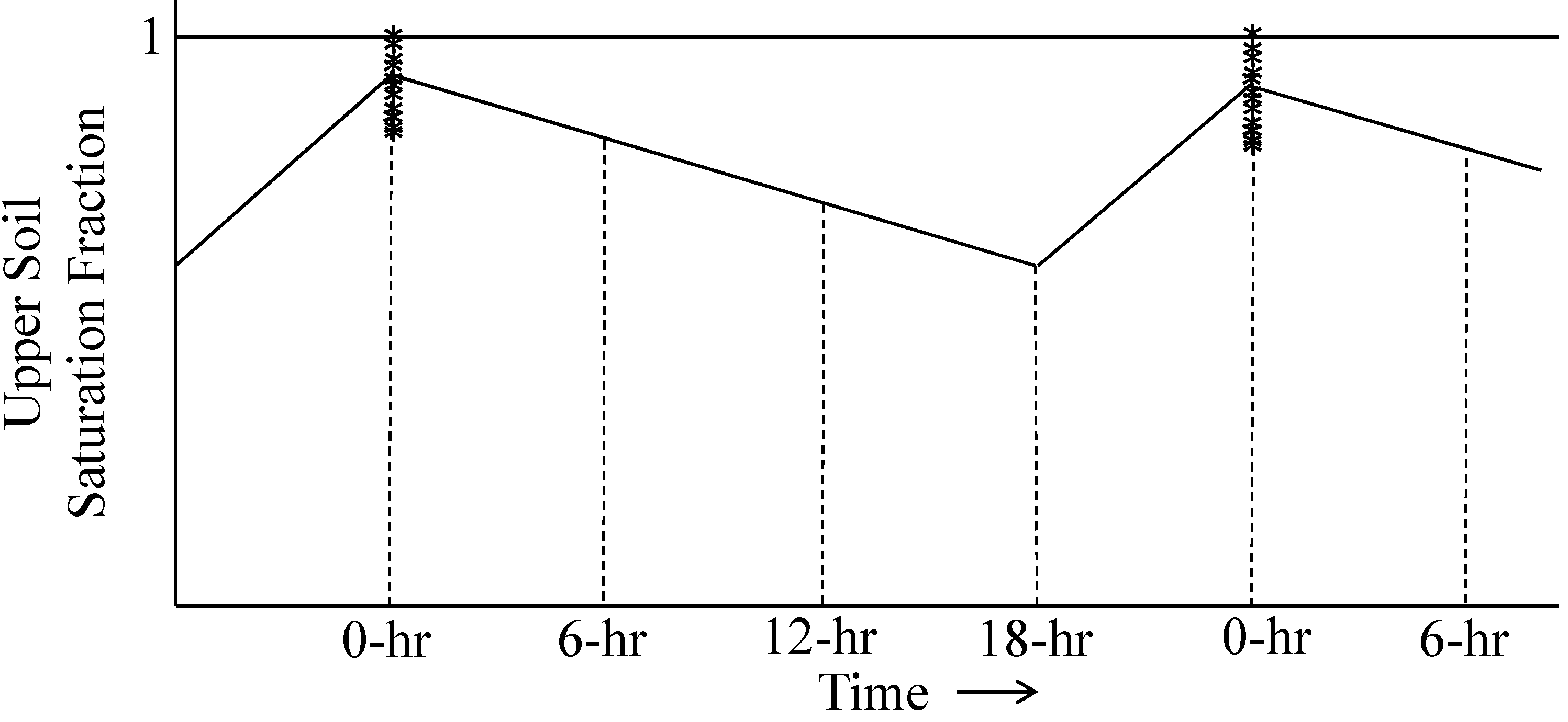
Model states are updated every six hours, concurrent with model forcing data; however, NASA MODIS Flood Maps are available once daily. Therefore, data assimilation occurred only at 00Z, the time of the MODIS data availability, at which time an ensemble of w’ estimates was obtained as discussed above. After the 00Z data assimilation, the mean of the generated ensemble members provides the initial condition for the soil-water model integration for the remaining six-hour intervals in that day (Figure 4).

Figure 4. Illustration of each Monte Carlo simulation (*) result, the averaging that occurs at each assimilation time-step, reflecting that inundation information is provided daily at 00Z.

Figure 4. Illustration of each Monte Carlo simulation (*) result, the averaging that occurs at each assimilation time-step, reflecting that inundation information is provided daily at 00Z.

Basin rainfall-runoff processes are represented through the continuous soil-moisture accounting hydrologic model developed by Georgakakos [21]. The structure of this hydrologic model retains memory of previous hydrologic conditions, which is ideal for the prediction of response to short duration precipitation inputs. In the model used [22], the upper soil zone consists of a tension water element, depleted only by evapotranspiration, and a gravitational water element depleted by evapotranspiration, percolation and interflow. The upper soil zone saturation fraction, w, is a function of the upper soil zone gravitational free, UZF, and tension water, UZT, fractions and capacities as follows:

$$w=\frac{UZ{F}_{fraction}UZ{F}_{capacity}+UZ{T}_{fraction}UZ{T}_{capacity}}{UZ{F}_{capacity}+UZ{T}_{capacity}}$$

(17)

It is necessary to map the mean of the corrected upper soil zone saturation fraction, E{w’}, back to hydrologic model states in order to use these as initial conditions for model integration. Given that the modeled and the mean of the corrected soil saturation fractions are known after the assimilation of the MODIS inundation fraction, their ratio may be set equal to the ratio of their definition as indicated in Equation (17). That is:

$$\frac{E\left\{w^{\prime }\right\}}{w}=\frac{UZ{F}_{fraction}^{\prime }UZ{F}_{capacity}+UZ{T}_{fraction}^{\prime }UZ{T}_{capacity}}{UZ{F}_{fraction}UZ{F}_{capacity}+UZ{T}_{fraction}UZ{T}_{capacity}}$$

(18)

where primed quantities represent the corrected fractions for the tension and gravitational water elements. To find unique estimates of the primed quantities in Equation (18) the additional constraint is set that the tension water element must be full (UZT_fraction = 1) before the gravitational water element contains any water. The estimated model states, UZF’ and UZT’, are then used as initial conditions for the model in the subsequent simulation time step.

Implementation of the solution procedure uses analytical expressions that are based on rewriting Equation (18) as follows:

X₁ B₁ + X₂ B₂ = A

(19)

with

X₁ = UZT’_fraction

(20)

X₂ = UZF’_fraction

(21)

B₁ = UZT_capacity

(22)

B₂ = UZF_capacity

(23)

A = (E{w’}/w)(UZT_fractionUZT_capacity + UZF_fractionUZF_capacity)

(24)

The solutions of Equation (19) for X₁ and X₂ are along a line that intersects the X₁-axis at (A/B₁) and the X₂-axis at (A/B₂). The determination of the estimates of X₁ and X₂ that also satisfy the constraint requiring filling of the tension water element first may be done using the following expressions:

X₁ = 1 & X₂ = ( A − B₁)/B₂; A/B₁ ≥ 1

(25)

X₁ = A/B₁ & X₂ = 0; A/B₁ < 1

(26)

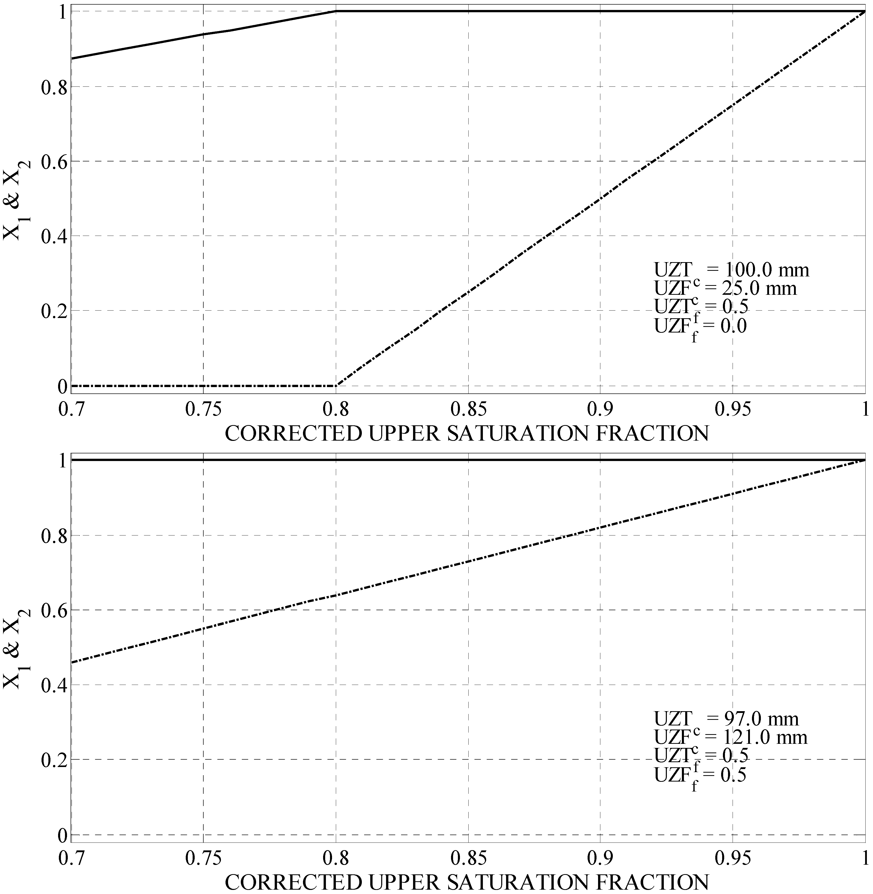
It is noted that the solution functions in Equations (25) and (26) are continuous for A = B₁. Figure 5 exemplifies the behavior of the solutions found as the E{w’} changes for two sets of fixed ratios UZT_fraction and UZF_fraction and for two different sets of upper zone tension and gravitational water element capacities). The upper panel is for a large tension water element while the lower panel is for a large gravitational water element. Corrected saturation fractions greater than 0.7 are used, in line with the assimilation of MODIS inundation fractions approaching one. Clearly the behavior of the solutions is very different for different parameters and model saturation fractions and for the same range of E{w’}.

Figure 5. Solutions of the Equations (25) and (26) as functions of the mean corrected model upper soil saturation fraction, E{w’}, for two different catchment parameters and model saturation fractions. Solid line is for X1 and dashed line is for X2.

Figure 5. Solutions of the Equations (25) and (26) as functions of the mean corrected model upper soil saturation fraction, E{w’}, for two different catchment parameters and model saturation fractions. Solid line is for X1 and dashed line is for X2.

3. Study Area

The region under analysis is hydrologically dominated by the Mekong River and covers much of mainland Southeast Asia, including all of Cambodia and most of Thailand, Laos, and Vietnam. By any set of measures, such as length, mean annual flow, the diversity of river plant and animal life or the size and diversity of aquatic resources, the Mekong River is one of the largest rivers in the world [23]. This region experiences very distinct rainy and dry seasons as a result of the Southwest Monsoon, the rainy season lasting from approximately May through October (Figure 6), based on 1961–1990 climatology [24].

Figure 6. Precipitation in Bangkok based on monthly averages for the 30-year period 1961–1990 [24].

Figure 6. Precipitation in Bangkok based on monthly averages for the 30-year period 1961–1990 [24].

The result is extensive inundation occurring in the latter half of the year along the Mekong River and main tributaries. Figure 7 illustrates that in addition to the flooding in 2011 being significantly above average, flooding occurred in 2000 with also severe consequences. One of the factors identified to have increased the severity of the 2011 flooding is deforestation leading to the erosion of hillsides which increased bed and water levels in rivers. In addition, the improper maintenance of the storm sewer system resulted in sewer clogging of that system, increasing inundation extent [25].

Figure 7. Mekong River flooding at Tan Chua gauge from 1 June through 11 November 1992, 1998, 2000, 2010, and 2011, along with the Average, the Flood Stage, and the Alarm Stage [26].

Figure 7. Mekong River flooding at Tan Chua gauge from 1 June through 11 November 1992, 1998, 2000, 2010, and 2011, along with the Average, the Flood Stage, and the Alarm Stage [26].

4. Data Opportunities and Constraints

Use of remote sensing from orbit to detect inundation extent has been proven to be closely correlated with ground measurements of river discharge [27,28,29,30,31,32]. In general, two types of remote sensors are suitable for detection of inundation, microwave and optical sensors. Microwave sensors such as Synthetic Aperture Radar were proven to be useful in mapping inundation extent under all weather conditions due to their ability to penetrate clouds. Observations from optical sensors such as Landsat Multispectral Scanner (MSS), Thematic Mapper/ Enhanced Thematic Mapper Plus (TM/ETM+; [33,34,35]), and SPOT [36] are common and easily acquired. While these products have very high spatial resolution, they have very low temporal resolution, with up to two weeks between observations. Although with lower spatial resolution, and frequent contamination due to cloud cover, the products from MODIS [37,38,39,40] and the Advanced Very High Resolution Radiometer (AVHRR) are also used to classify flood areas [2,41,42,43,44]. Validation of MODIS-derived inundation extent mapping is done through comparison with either other remotely sensed data such as Landsat [2,3] or stream gauge measurements associated with flood peak detection [4,21]. Over the Cambodian and Vietnamese Mekong Delta region Sakamoto et al. [2] found that during five annual flooding seasons MODIS and RADARSAT-derived inundation maps had coefficients of determination (R2) values of from 0.89 to 0.92, and compared with Landsat-derived results R2 values of 0.77 to 0.97 were found.

The Moderate Resolution Imaging Spectroradiometer (MODIS) instrument sits aboard both the Aqua and Terra satellites. Due to its worldwide availability, no cost, and daily coverage, MODIS is the ideal tool for detecting inundated areas [2]. NASA Goddard’s Office of Applied Science (GSFC OAS) is working to operationalize near real-time global flood mapping using the existing twice daily overpass of the MODIS instrument on both the Terra and Aqua satellites [21]. The orbits of these two satellites are timed such that between them, they view the entire earth’s surface every one to two days, acquiring data in 36 spectral bands, or groups of wavelengths. The NASA GSFC OAS, in collaboration with the Dartmouth Flood Observatory, has developed the Near Real-Time Global Flood Mapping Project. Flood maps are produced in 10 × 10 degree tiles with a pixel size of 0.002197 degree square (~250 m). Gridded products are typically 4551 × 4551 pixels in size; however, some data sets vary by 1 to 2 pixels. The Global Flood Mapping Project produces a MODIS Surface Water (MSW) product, indicating where standing water is located on the globe, a MODIS Flood Water (MFW) product, which is the MODIS Surface Water product with the reference water layer subtracted, and a MODIS Water Product (MWP), that combines the MSW and MFW products. The NASA GSFC OAS, in developing the MWP, is capable of using a composite product that requires a predetermined number of observations (e.g., three consecutive days) in order to label a pixel as water. As is the case with all passive sensors, MODIS data is limited by cloud cover during continuous rainy days; therefore, MWP maps assign “Insufficient data” designation to those pixels obscured by clouds.

The Global Flood Mapping Project team is also capable of using terrain, cloud, or both terrain and cloud shadow masking. The Global Flood Mapping Project team currently produce two standard MWP products, a two-day consecutive and three-day consecutive observation requirement, both having terrain masking applied. Currently, cloud masking is only available on single-day products.

Uncertainty in the MWP may result from cloudiness. Despite the fact that clouds may appear spectrally similar to standing water, all water detections are currently kept. However, the MOD 35 Cloud Mask product is used for quality control through its use in development of the “Insufficient Data” layer. To date, the cloud mask (MOD 35) is at a 1km grid resolution, which may result in additional quality control issues. Shadows are also spectrally similar to standing water and therefore must be distinguished. As of version 4.7, a cloud shadow masking algorithm is used that combines the cloud locations from MOD 35 and the cloud height from MOD 06 to estimate the cloud location on the ground. However, the Global Flood Mapping Project team has determined that it is detrimental to apply cloud masking to the composite products, as many real water observations may be masked due to the buffering around the detected clouds.

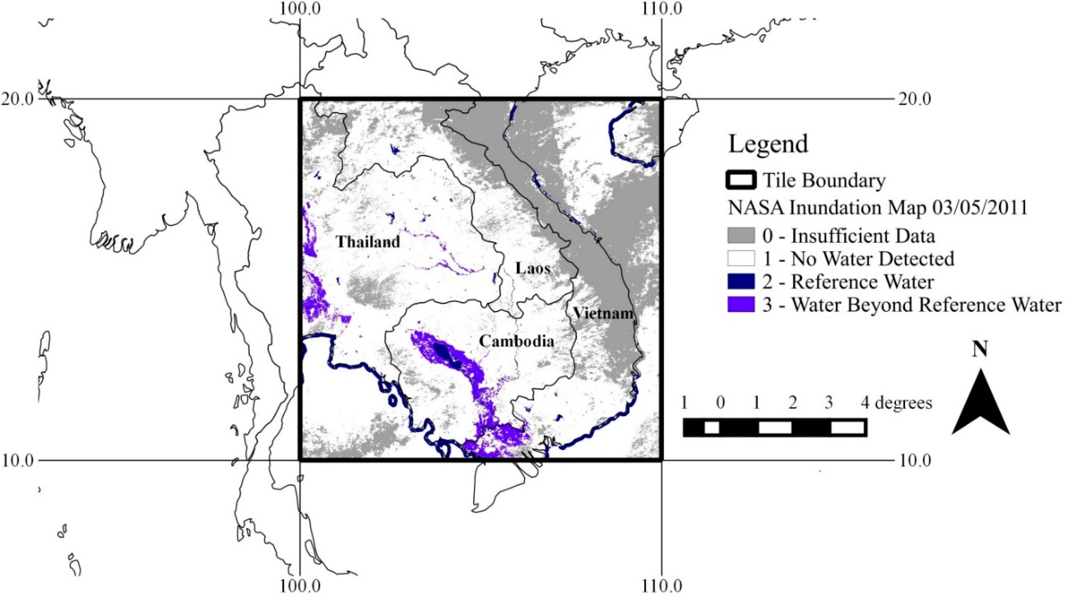
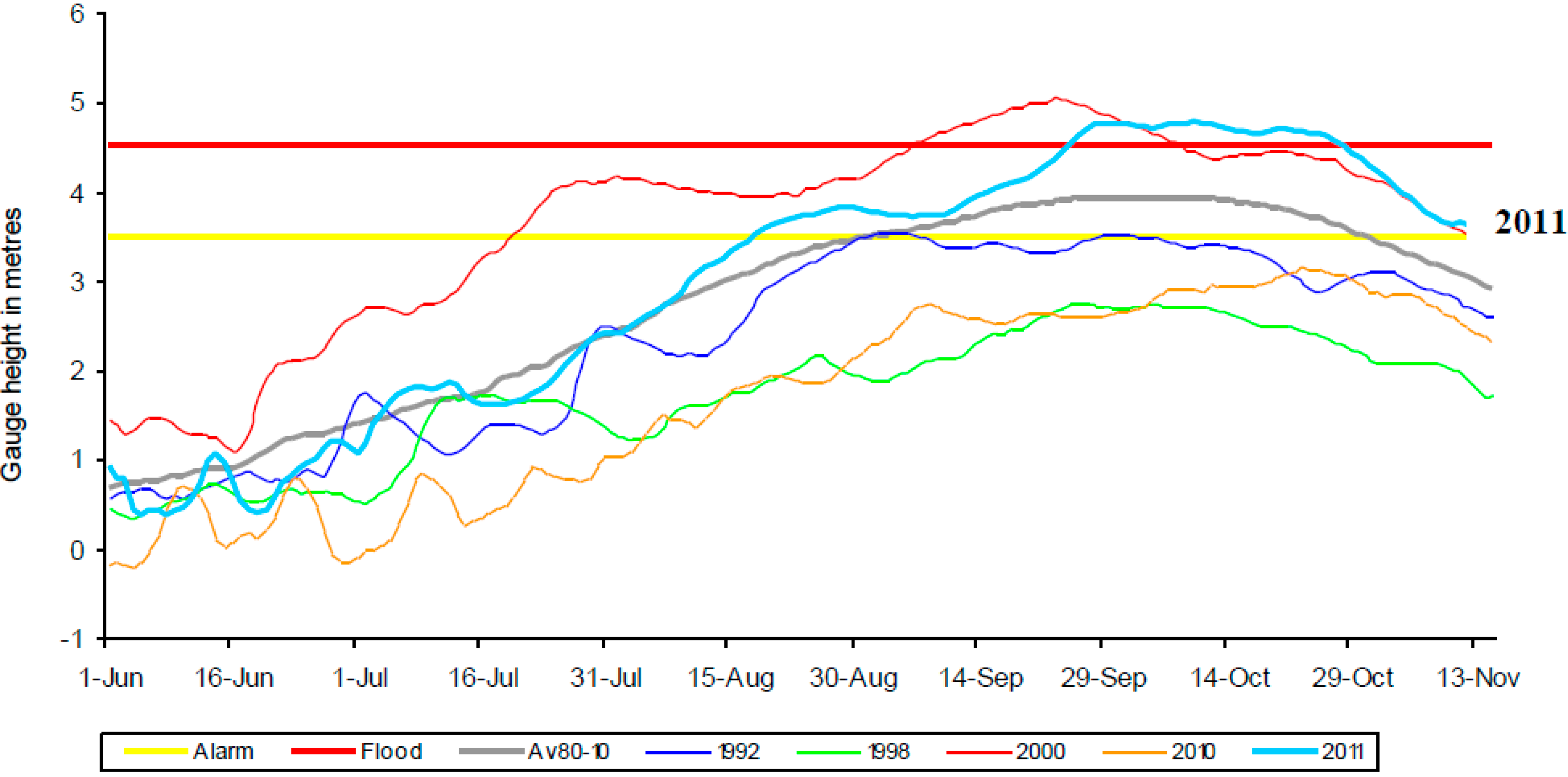
Working with staff at NASA Goddard’s Office of Applied Science, the Hydrologic Research Center (HRC) obtained Near Real-time (NRT) Global MODIS Flood Maps for the 10-degree tile with coordinates 100E and 20N in the tile’s northwest corner, covering all of Cambodia along with areas of Vietnam, Thailand, and Laos (Figure 8). Tile products are in raster format, 4551 × 4551 pixels in size. However, the number of pixels does vary by one to two pixels depending on the particular input data. Flood maps were obtained between 3 July and 31 December 2011 to cover the period of extensive flooding that occurred on the Mekong River (Figure 7).

Figure 8. NASA Flood Map 10 × 10 degree tile over Southeast Asia with tile cell values.

Figure 8. NASA Flood Map 10 × 10 degree tile over Southeast Asia with tile cell values.

The NASA Global Flood Map raster products assign a value between 0 and 3 to each pixel: 0 representing insufficient data to make water determination, 1 for no water detected, 2 meaning water was detected, but is coinciding with reference water, and 3 referring to areas where water was detected, but is not coinciding with reference water. Insufficient data may be the result of clouds, missing images, swath gaps, or bad data values. The FFG system sub-basin delineation accounts for the existence of reference water, as sub-basins do not include rivers and lakes. In order to transfer pixel values to the fractional inundation of individual sub-basins, the centroid of each pixel was mapped to each sub-basin in order to assign individual pixels to a given sub-basin. The frequency of each pixel value within each sub-basin was then determined. Due to the fact that sub-basins exclude reference water, sub-basin standing water was considered to include pixel designations, Reference Water and Water beyond Reference Water. Therefore, percent sub-basin inundation is calculated based on the number of pixels with values of 2 and 3, divided by the number of pixels with values of 1, 2, or 3, representing those pixels for which data is available. Percent inundation varies widely in both the spatial and temporal domain under investigation.

The HRC maintains a database of historical mean aerial precipitation estimates for the Mekong River region, associated with the Mekong River Commission (MRC) Flash Flood Guidance System (MRCFFG), in use by the MRC. This precipitation database was used to run a stand-alone adaptation of the Sacramento soil moisture accounting model for rainfall-runoff generation [14] used in the operational MRCFFG system for those watershed sub-basins within the NASA flood map tile. Parameters for sub-basin runoff generation were determined through the approach described in Duan et al. [45].

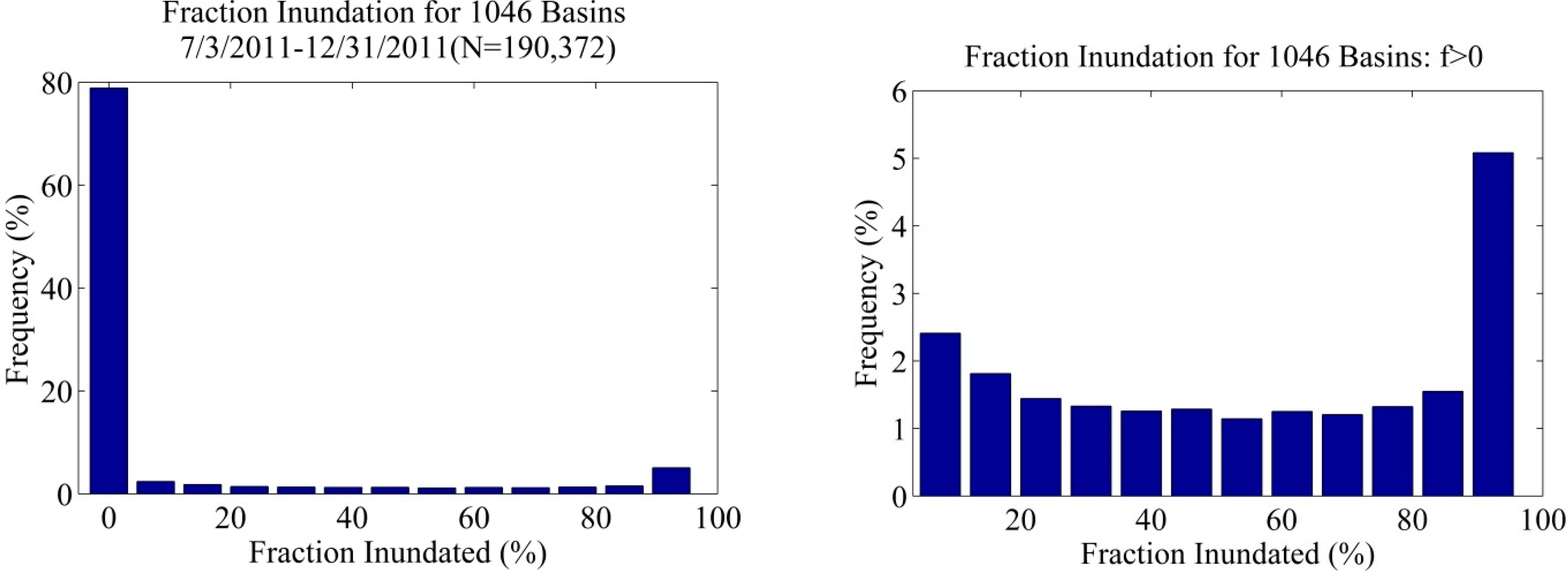
To determine the feasibility of using the NASA Flood Map product to improve the flash flood guidance system response in inundated basins, first we looked at a 30 km buffer around the low lying region associated with the Chao Phraya and Mekong Rivers, and the Tonle Sap, an inland lake (Figure 9). In order to assess the possible impact of assimilating fractional basin inundation for these 1046 basins within the 30 km buffer, the fractional inundation was calculated for each day during the second half of 2011, from 3 July to 31 December. Figure 10 illustrates that over the 190,372 basin-days, nearly 80% of those samples had no inundation. However, Figure 10 also shows that approximately 7% of the basin-days had over 80% inundation, suggesting that, although limited, assimilation of this data has the potential to have significant impacts to specific locations.

Figure 9. Mekong River Commission (MRC) Flash Flood Guidance (FFG) basins (n = 1046) within a 30 km buffer of regional low-lying areas.

Figure 9. Mekong River Commission (MRC) Flash Flood Guidance (FFG) basins (n = 1046) within a 30 km buffer of regional low-lying areas.

Figure 10. Frequency of fractional inundation for low lying regions of southeast Asia over the study time period (left), and the frequency of percent inundated, f, greater than zero for study time period (right).

Figure 10. Frequency of fractional inundation for low lying regions of southeast Asia over the study time period (left), and the frequency of percent inundated, f, greater than zero for study time period (right).

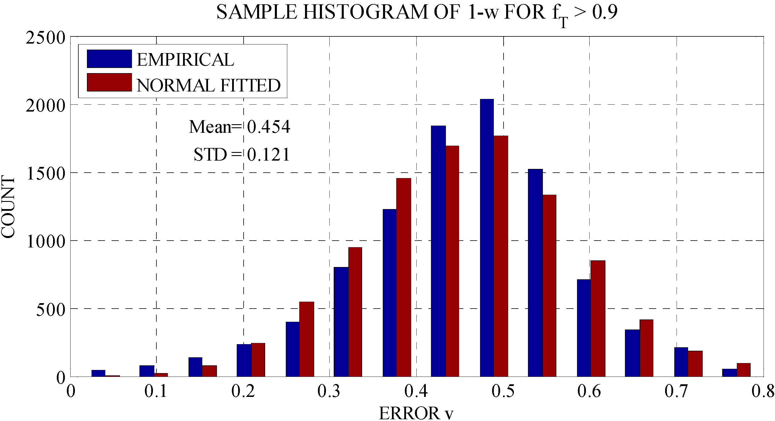
Next, the fractional inundation threshold (f_T = 0.9) was used to estimate the distribution of the model error (v in Equation (8)) in order to determine parameters for the Monte Carlo ensemble analysis. Figure 11 illustrates that the model error distribution is nearly normal, although skewed toward lower values. In order to represent the paired uncertainty of both modeled soil moisture, w, and model error, v, modeled soil moisture associated with model errors used in development of Figure 11, Equation (8), were divided in to 100 equally sized bins. The statistical moments of the model error, were then calculated and used to derive 100 normally distributed random error terms ζ from Equations (11) and (12) for Monte Carlo ensemble simulation through Equation (9).

Figure 11. Sample frequency of model error v.

Figure 11. Sample frequency of model error v.

5. Results

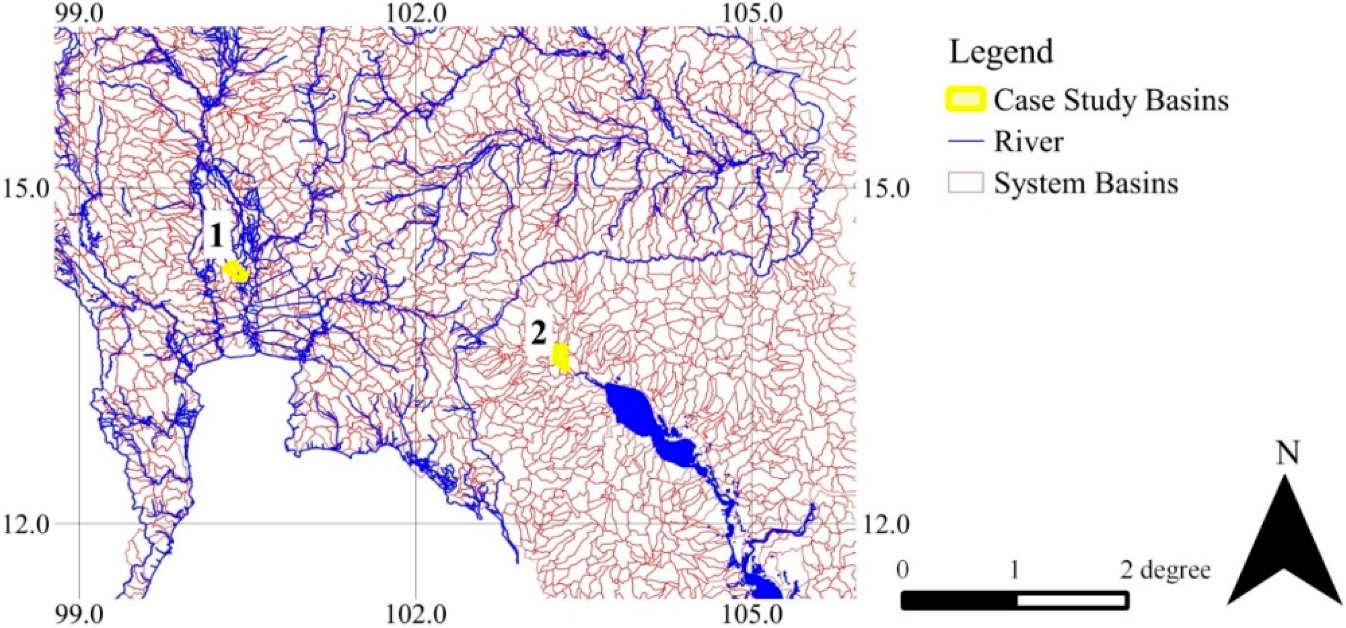
In order to assess the impact of flood map assimilation, two basins were chosen for further analysis. Both basins were chosen to represent low lying areas in the region (Figure 12). Table 1 describes the basin characteristics of each test basin, reflecting their similar characters of low elevation, relatively gentle slopes, and very deep soils. In addition, these basins were chosen based on the fact that while being low lying and experiencing inundation, they are not in the littoral zone of adjacent water bodies, where changes to water levels would directly impact flooding in the basin.

Figure 12. The two case-study basins: (a) just upstream of Bangkok near the Chao Phraya River (31245), and (b) upstream of the Tonle Sap Lake in Cambodia (10171).

Figure 12. The two case-study basins: (a) just upstream of Bangkok near the Chao Phraya River (31245), and (b) upstream of the Tonle Sap Lake in Cambodia (10171).

Table 1. Case study basin characteristics.

Basin ID No.	31245	10171
Location	Bangkok	Tonle Sap Lake Region
Soil Texture	Silty Clay	Silt
Soil Depth	Very Deep	Very Deep
Land Use/Land Classification	Cropland/Woodland/Grassland	Grassland
Elevation (m)	6	10
Area (km2)	162	164
Channel Length (km)	32.2	26.8
Channel Slope (%)	0.31	0.4

Table 1. Case study basin characteristics.

Basin ID No.	31245	10171
Location	Bangkok	Tonle Sap Lake Region
Soil Texture	Silty Clay	Silt
Soil Depth	Very Deep	Very Deep
Land Use/Land Classification	Cropland/Woodland/Grassland	Grassland
Elevation (m)	6	10
Area (km2)	162	164
Channel Length (km)	32.2	26.8
Channel Slope (%)	0.31	0.4

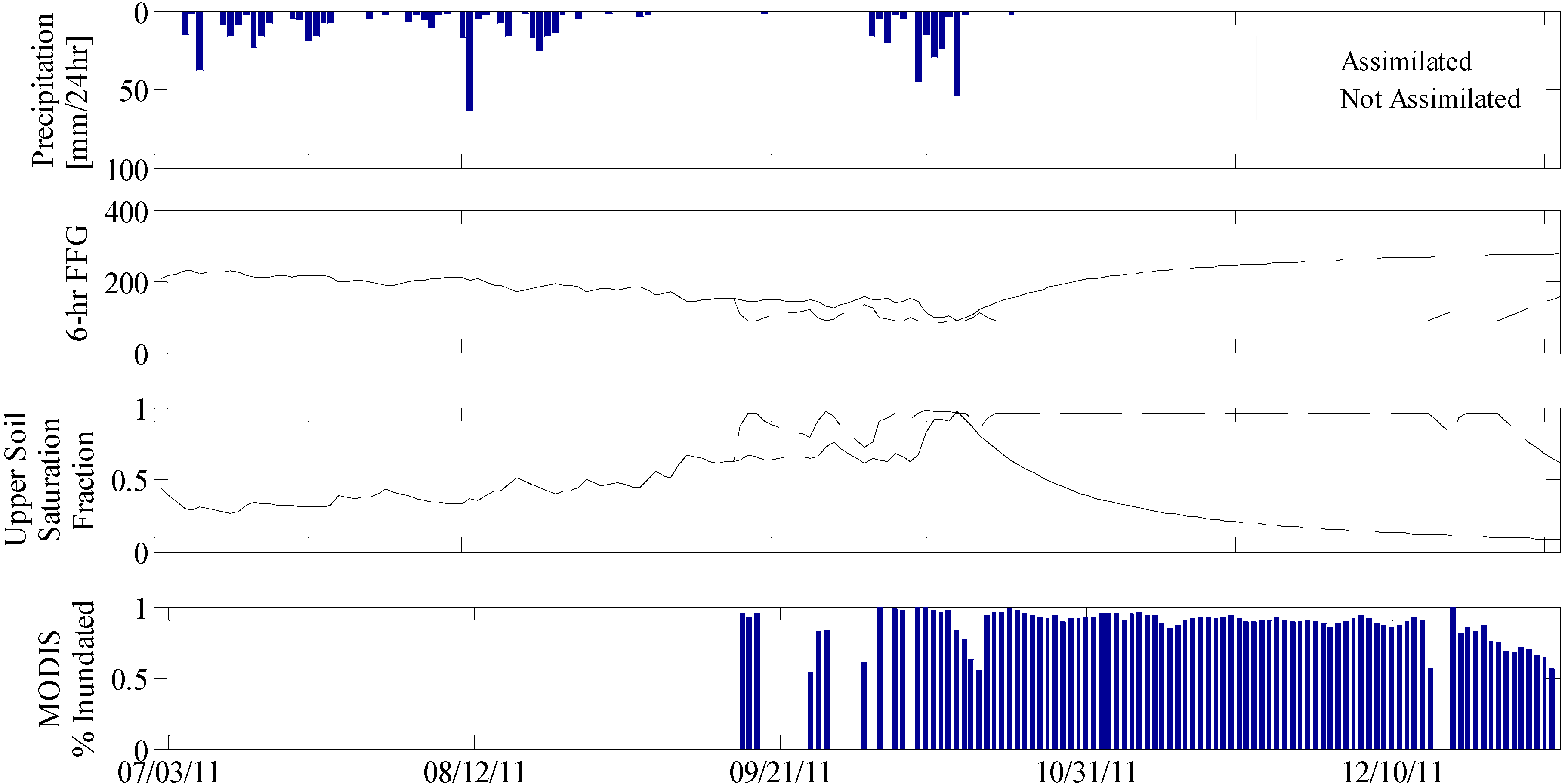
Figure 13 illustrates the conditions observed in Basin No. 31245 during the analysis period illustrate the stark contrast between rainy and dry precipitation regimes (Figure 13a), and inundated and not inundated surface conditions (Figure 13d). Inundation does not occur until well after the concentrated mass of precipitation is long over, and the degree of inundation proceeds from zero to almost entirely inundated very rapidly. The soil saturation fraction represents the extent to which the upper zone gravitational and tension water capacities are met. Figure 13c illustrates that the soil saturation fraction without assimilation tracks the rainfall input by dropping concurrently with the absence of precipitation. This figure also shows that with assimilation of the satellite inundation data, when above the inundation threshold (f_T = 0.75) and using a Monte Carlo ensemble analysis, in the mean, the system maintains high soil moisture in the basin, reflecting the extensive inundation.

Figure 13. Forcing variables and modeling results for the hydrologic response of Basin No. 31245: (a) precipitation, (b) the 6-hr Flash Flood Guidance value (in mm/6hrs), (c) soil moisture saturation fraction, and (d) the fraction inundated.

Figure 13. Forcing variables and modeling results for the hydrologic response of Basin No. 31245: (a) precipitation, (b) the 6-hr Flash Flood Guidance value (in mm/6hrs), (c) soil moisture saturation fraction, and (d) the fraction inundated.

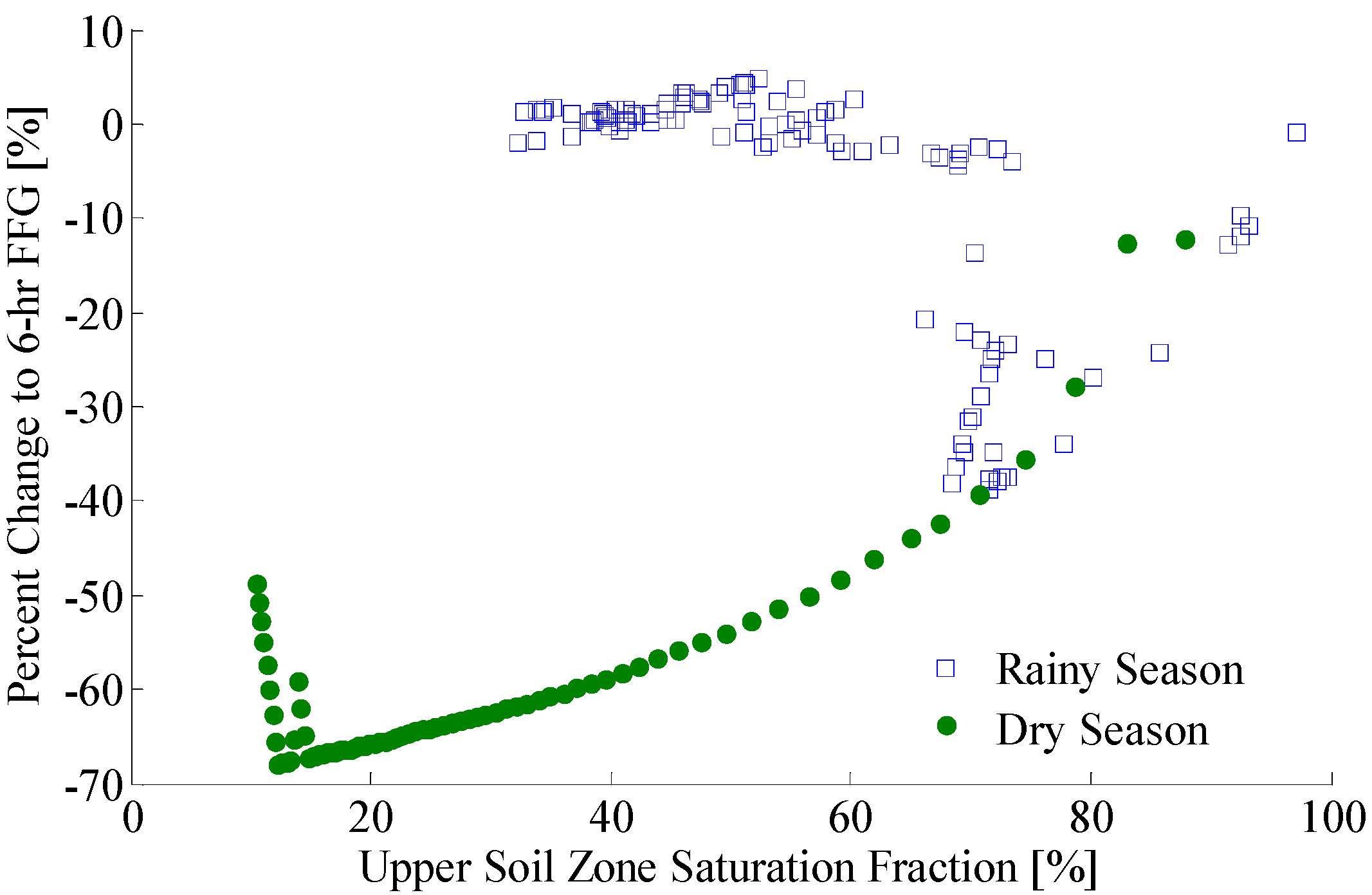
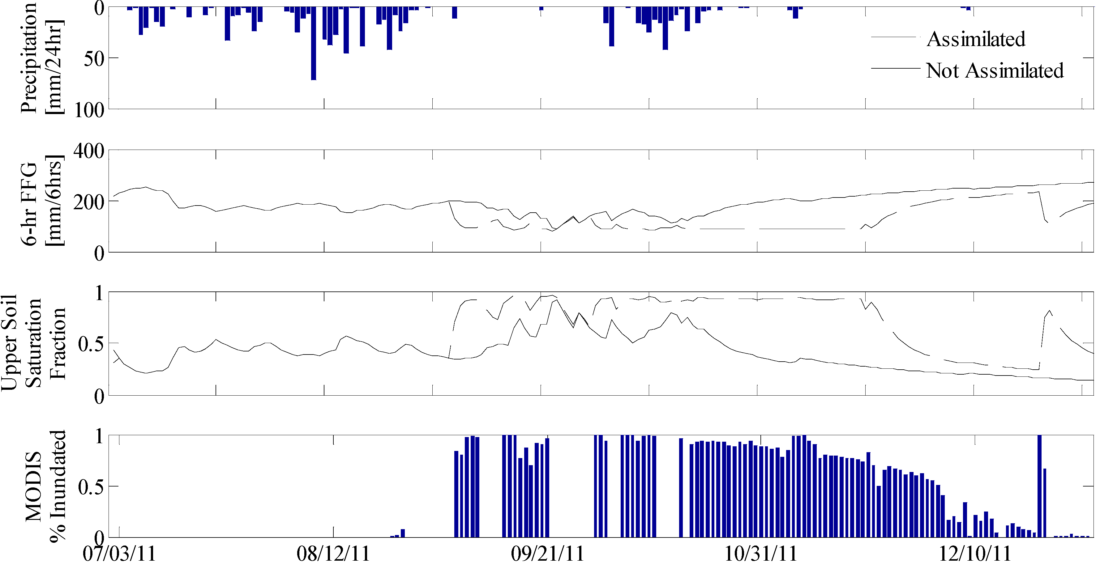
The direct impact of flood map assimilation onto the MRCFFG system is shown in Figure 14, where the percent change in FFG values dramatically decreases (representing an increase in the likelihood of a flash flood) with decreases in model saturation fraction. Figure 14 also illustrates the dramatic difference between wet and dry season impacts, whereby in the wet season the majority of records have a percent change of less than 10, showing little impact of assimilation. Conversely, in the dry season, when upper soil zone saturation fractions are low prior to assimilation, changes to 6-hr FFG values go from −30% to −70% change. The results of the second basin are analogous, with the exception that the percent of the basin inundate decreases from full inundation to nearly dry ground during the dry season (Figure 15). This decrease highlights the role of the assimilation threshold, when at approximately mid-November this threshold is breached and assimilation ceases. Over the subsequent weeks considerable drying of the soil is seen, until mid-December when the threshold is crossed by a significant amount of inundation and assimilation occurs again.

Figure 14. Impact of flood map assimilation on the results of the FFG value for Basin No. 31245, as a function of the model soil saturation fraction (with no assimilation). More negative values indicate that less water is required to declare a flash flood warning or alert.

Figure 14. Impact of flood map assimilation on the results of the FFG value for Basin No. 31245, as a function of the model soil saturation fraction (with no assimilation). More negative values indicate that less water is required to declare a flash flood warning or alert.

Figure 15. Forcing variables and modeling results for the hydrologic response of Basin No. 10171: (a) precipitation, (b) the 6-hr Flash Flood Guidance value (in mm/6hrs), (c) soil moisture saturation fraction, and (d) the fraction inundated.

Figure 15. Forcing variables and modeling results for the hydrologic response of Basin No. 10171: (a) precipitation, (b) the 6-hr Flash Flood Guidance value (in mm/6hrs), (c) soil moisture saturation fraction, and (d) the fraction inundated.

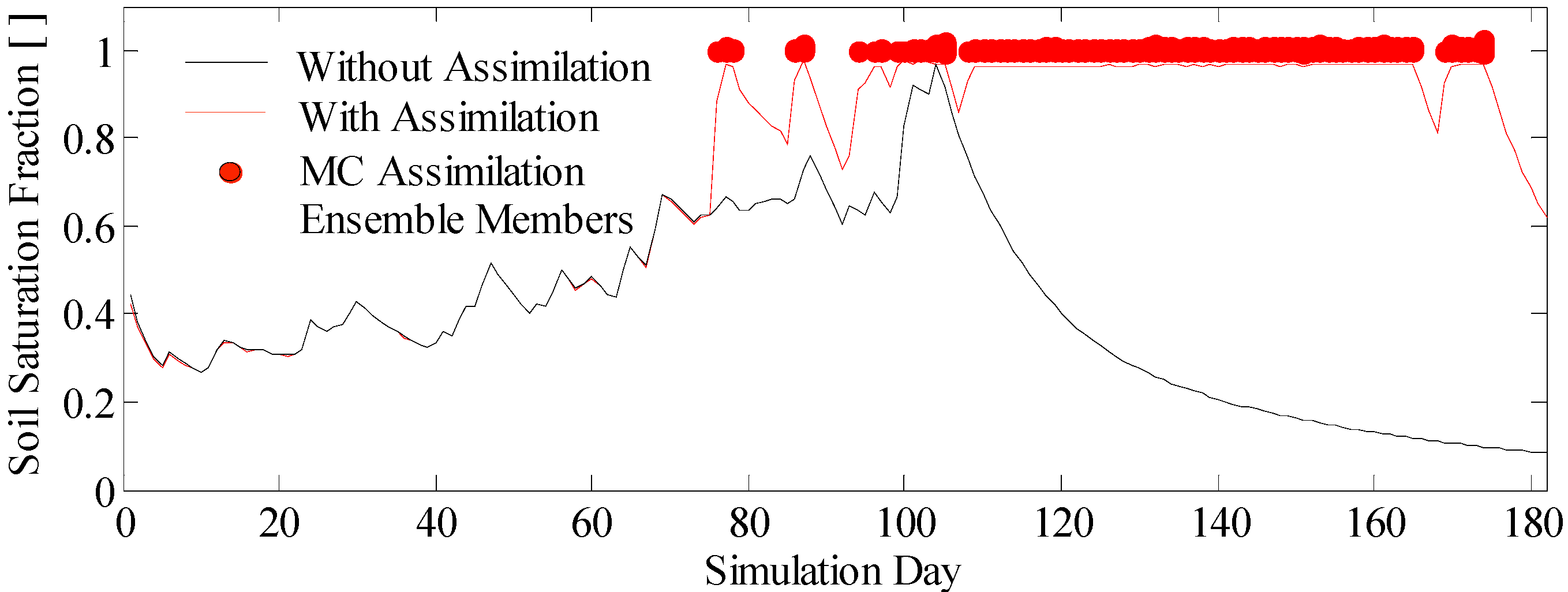
Figure 16 illustrates that in many cases when inundation events exceeding the threshold for assimilation are followed by periods without inundation above the threshold, the result is a predicted drying of soils. In addition, modeled soil moisture under-predicts the soil moisture conditions due to drying during the 6-, 12-, and 18-hour model time steps (Figure 4). Note that slight exceedance of the value of 1 is observed in some cases by some of the assimilated members of the ensemble due to the use of a continuous normal distribution for the input error values (ζ ), and for values of modeled saturation fraction (w) near 1. The use of a compound normal distribution with a mass at 1 would avoid such exceedance, but the effect in the mean and the variance is found to be negligible for this application.

Figure 16. Soil saturation fraction with no assimilation (black line), each member of the Monte Carlo ensemble estimates after assimilation (red dot), and the soil saturation fraction for each day after data assimilation (red line).

Figure 16. Soil saturation fraction with no assimilation (black line), each member of the Monte Carlo ensemble estimates after assimilation (red dot), and the soil saturation fraction for each day after data assimilation (red line).

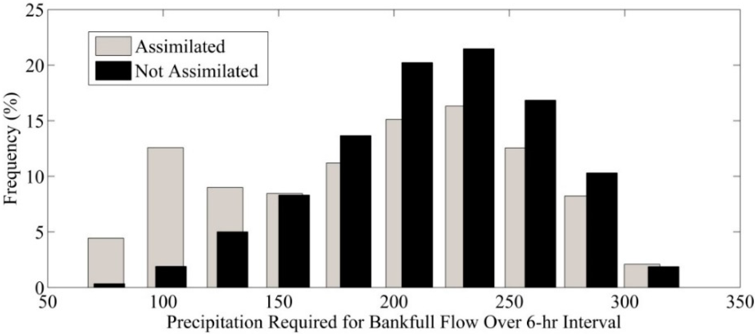
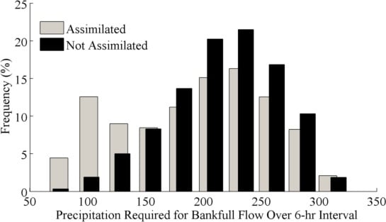
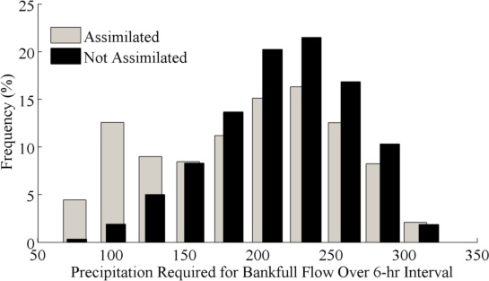
Within the 1045 basins located in a 30-km buffer around the Chao Phraya and Mekong Rivers (Figure 9), approximately 350 basins experience at least one day of fractional inundation exceeding 0.75. Figure 17 illustrates the frequency of FFG values in different bins, both with and without assimilating the NASA satellite flood map product into the MRCFFG system from 3 July to 31 December 2011. It is clear that assimilation results in an overall decrease in FFG values, where there are fewer records with high FFG values and more records with low FFG values. Approximately 44% more basin-days have lower FFG values as compared to the baseline of no assimilation, meaning that during those basin-days significantly less rainfall was required for the issuance of a flash flood warning. In addition, assimilation results in a bimodal distribution of FFG values, as compared to the unimodal distribution prior to assimilation.

Figure 17. Frequency of 6-hr FFG values for ~350 basins where the inundation fraction exceeds 0.75.

Figure 17. Frequency of 6-hr FFG values for ~350 basins where the inundation fraction exceeds 0.75.

6. Discussion

Results from the strategy tested for assimilation of inundation maps into the HRC Flash Flood Guidance System illustrate that there is a significant disconnect between the conditions of many of the lowland basins of the Mekong and Chao Phraya river and delta systems and their representation in the HRC Flash Flood Guidance System. Figure 13 and Figure 15 show that, despite the presence of large areas of standing water, the system modeling strategy results in relatively dry soils. Inundation maps developed by NASA for 2011, a season of historic flooding, clearly delineate the large areas of inundation found in the lowland areas associated with the Mekong and Chao Phraya Rivers (Figure 8), despite little or no rainfall in those regions (Figure 13 and Figure 15).

The results of assimilation on the likelihood that a flash flood warning should be issued are dramatic. Throughout most of the dry season in 2011, there are many basins like the two used for illustration that experienced flooding and would be very prone to flash flooding, given that additional rainfall occurred over those basins. This strategy assumes inherently that there is more uncertainty in the modeled soil moisture than the uncertainty associated with the NASA inundation maps. Within model predictions, uncertainty exists primarily within the model representation of soil saturation fraction due to parameter uncertainty associated with soil, land use, and vegetation characteristics and integration of watersheds, in satellite precipitation estimates that are known to have large errors, and the uncertainty associated with data assimilation methods. An examination of the data assimilation uncertainty illustrates that over the duration of the analysis time period, ensemble predictions resulted in a mean upper zone soil saturation fraction, E{w’}, of 0.993, with a standard deviation of 0.019, reflecting that relatively little uncertainty exists for the assimilation of satellite observations.

In order to maximize the opportunity to assimilate inundation observations, the fractional inundation threshold (f_T) was lower than the threshold used in determining which basin-days would be used to develop statistical error relationships used in the Monte Carlo procedure. The fractional threshold used for deriving the Monte Carlo parameters may be more constrained than that used during assimilation, as there is much less uncertainty associated with the NASA MWP maps than with all of the combined uncertainties in the hydrologic model forcing and parameterization. Therefore, a lower fractional inundation threshold for assimilation, of 0.75 representing three-quarters of the basin being inundated, allows the maximum amount of information possible used within the constraints of the derived assimilation strategy. It is noted that the soil saturation fraction results illustrated in Figure 14 constitute a temporal daily average of the mean of the 100-member ensemble at 00Z and the model results at 06Z, 12Z and 18Z, with the constraint that the soil saturation fraction cannot exceed unity.

Finally, Figure 17 illustrates that assimilation of inundation data results in a bimodal distribution of FFG values reflecting changes that occur only when inundation exceeds the set threshold value. In contrast, the model without assimilation has a unimodal distribution of FFG values suggesting that model response is proportionate to the single forcing of precipitation values.

7. Conclusions

Although limited in spatial and temporal application, assimilation of the NASA flood map into the HRC FFG system results in a more accurate depiction of those physical conditions occurring at the basin level. During the time period investigated, no flash floods occurred; therefore, we were not able to empirically validate the impact of assimilation. However, Figure 13b illustrates the impact of the assimilated data on the flash flood guidance (FFG) value, reflecting the fact that post-assimilation, significantly less rainfall is required to increase the likelihood of a flash flood. This result is consistent with the fact that large areas of the basin were inundated.

Upon implementation of this assimilation strategy in to the HRC operational systems, after several rainy seasons, authors will assess changes to the probability of detection of actual flash flood events, and have the opportunity to validate the assertion that inundation map assimilation reduces the likelihood of missing flash flood events, while also not increasing the likelihood of false warnings. One of the limitations of many surface water hydrology models, and reflected in the HRC’s operational systems, is the absence of inputs from groundwater, and other sources of water outside of the basin under examination. Clearly the source of inundation, in the context of the basins studied, is outside of the individual basin domain and its precipitation forcing. Large river flooding and tributary backwater effects are the most likely sources of inundation. Therefore, the basin-based modeling strategy used in operational flash-flood guidance systems does not account for these sources of water. Assimilation of the NASA Flood Map provides the ability to include water inflows from outside any particular basin that greatly influences the conditions of that basin.

The NASA Flood Map program has a wide range of utility from large flood warnings, to estimating flow rates in ungauged basins, to improving flash flood forecasting. There are a number of steps required to approach operational implementation of the elaborated strategy. Firstly, there is a significant amount of preprocessing that is done both within the Flash Flood Guidance System and to the NASA Flood Maps, in order to assimilate them in to the system. Monte Carlo ensemble prediction strategies must be optimized to minimize the time and computation intensity of application to avoid slowing down the production of system products that are required to have short latencies for warning efficacy.

There is also much opportunity for improvement of satellite derived flood mapping products. NASA is working to improve the reliability, accuracy, and precision of flood map products. It is clear that many of the low lying areas around the world experience seasonal flooding. In the region examined herein, annually the Mekong River rises in response to the rainy season. This increase in water level creates backwater effects into the Tonle Sap Lake and surrounding basins. This type of dynamic system requires that reference water layers be dynamic in order to ensure the accurate distinction between reference water and that water beyond the reference water. Secondly, many of the low lying areas around the world, and in Southeast Asia in particular, are used for rice paddy farming and are seasonal wetlands that experience severe flooding that underlies heavy vegetation. Finally, the use of Kalman Filtering to assimilate inundation observations into hydrologic models will provide the ability to use any fractional basin inundation value to update the soil moisture state variables.