Ground Surface Response to Geothermal Drilling and the Following Counteractions in Staufen im Breisgau (Germany) Investigated by TerraSAR-X Time Series Analysis and Geophysical Modeling

Abstract
:1. Introduction

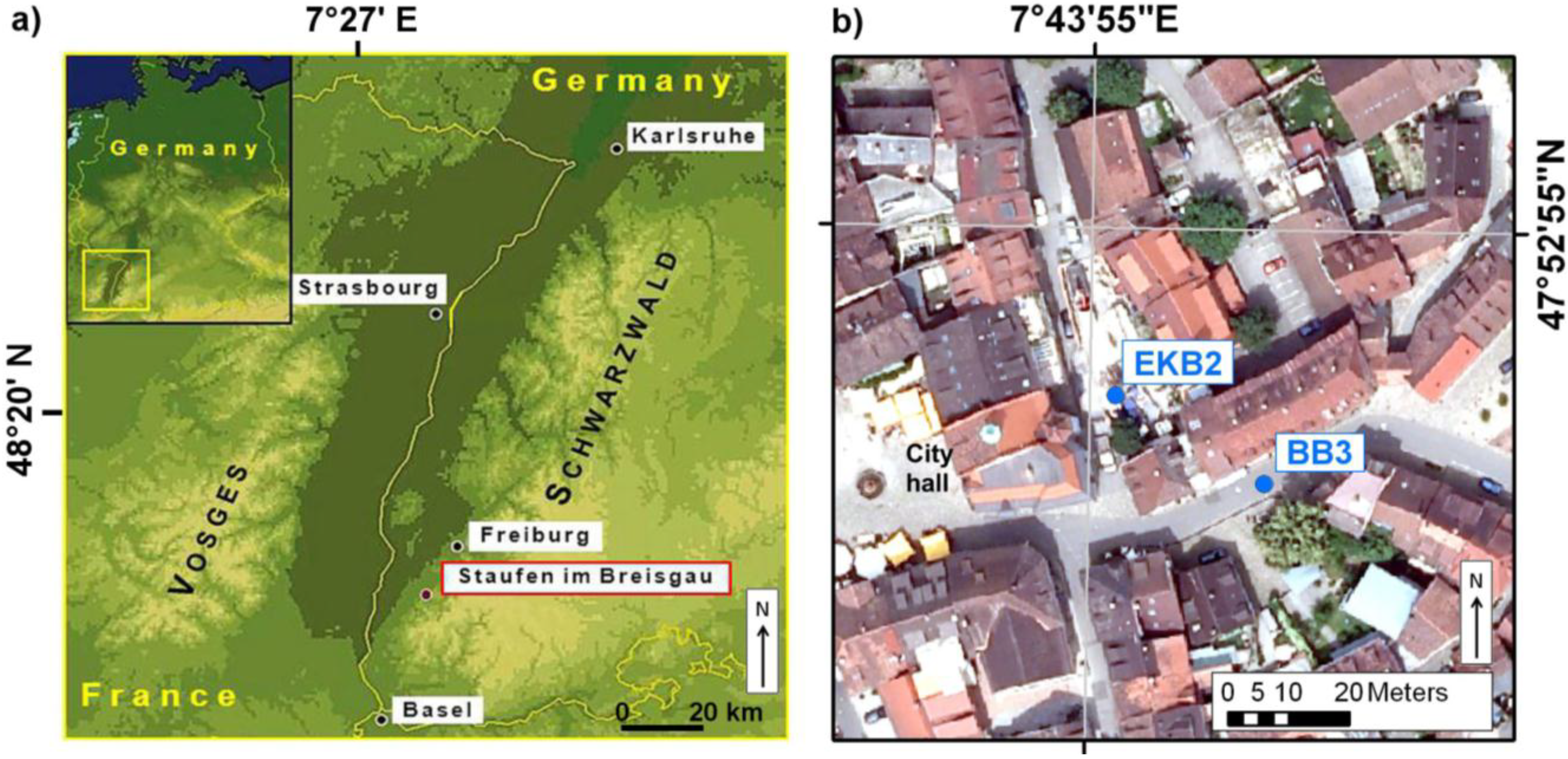
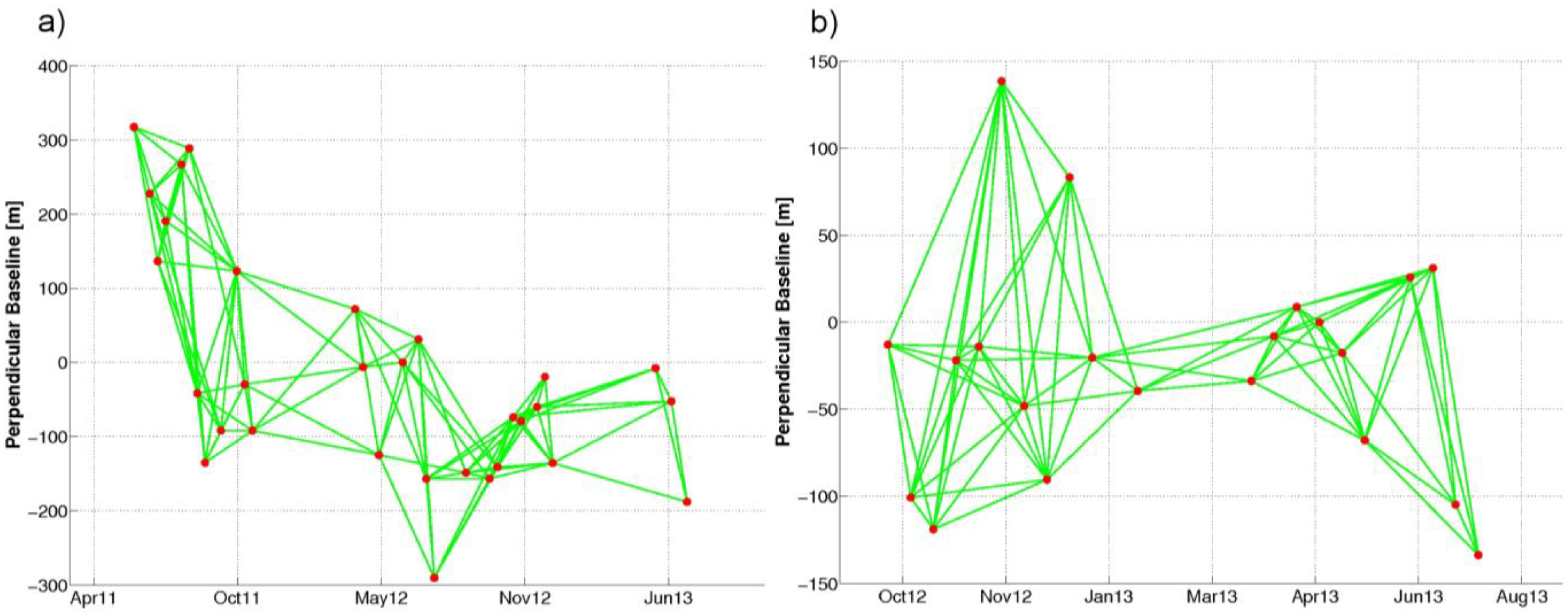
2. Data
3. Methodology
3.1. InSAR
3.2. Source Modeling


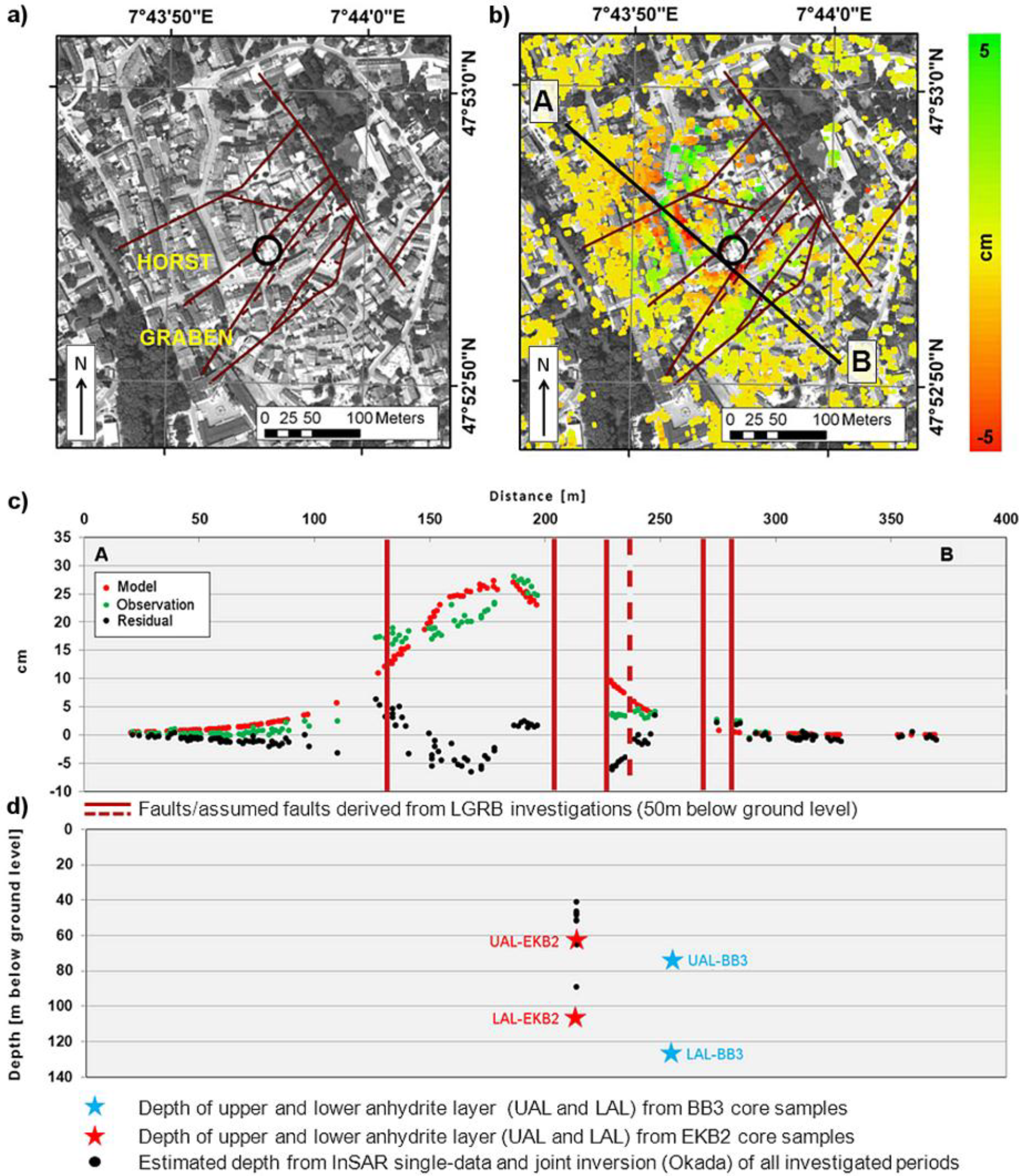
| Boundaries | Length (km) | Width (km) | Depth (km) | Dip (°) | Strike (°) |
|---|---|---|---|---|---|
| Lower Boundary | 0 | 0 | 0 | −20 | 0 |
| Upper Boundary | 0.5 | 0.5 | 1 | 0 | 90 |
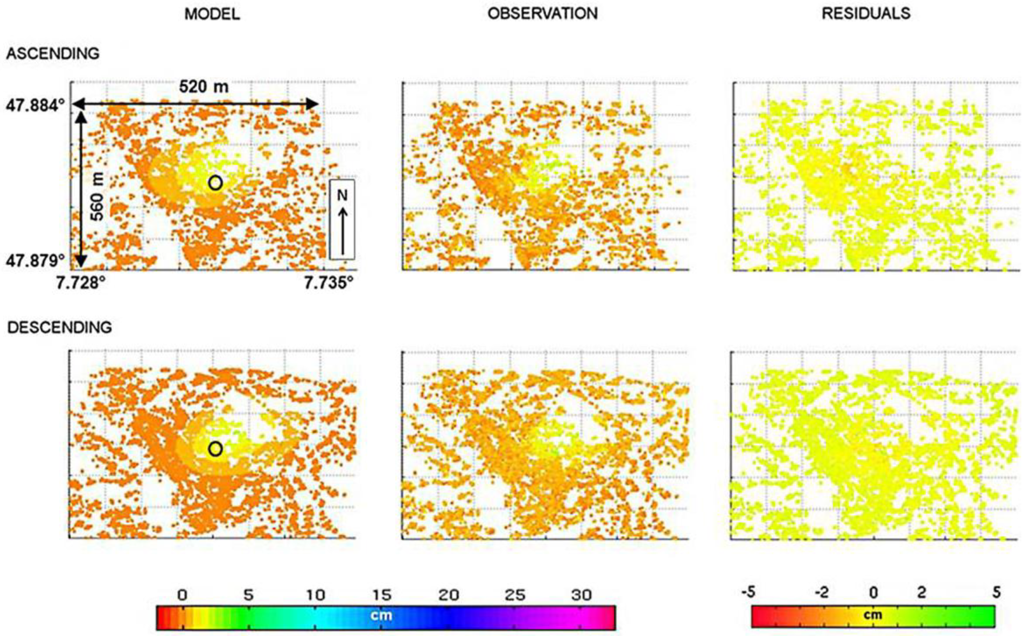
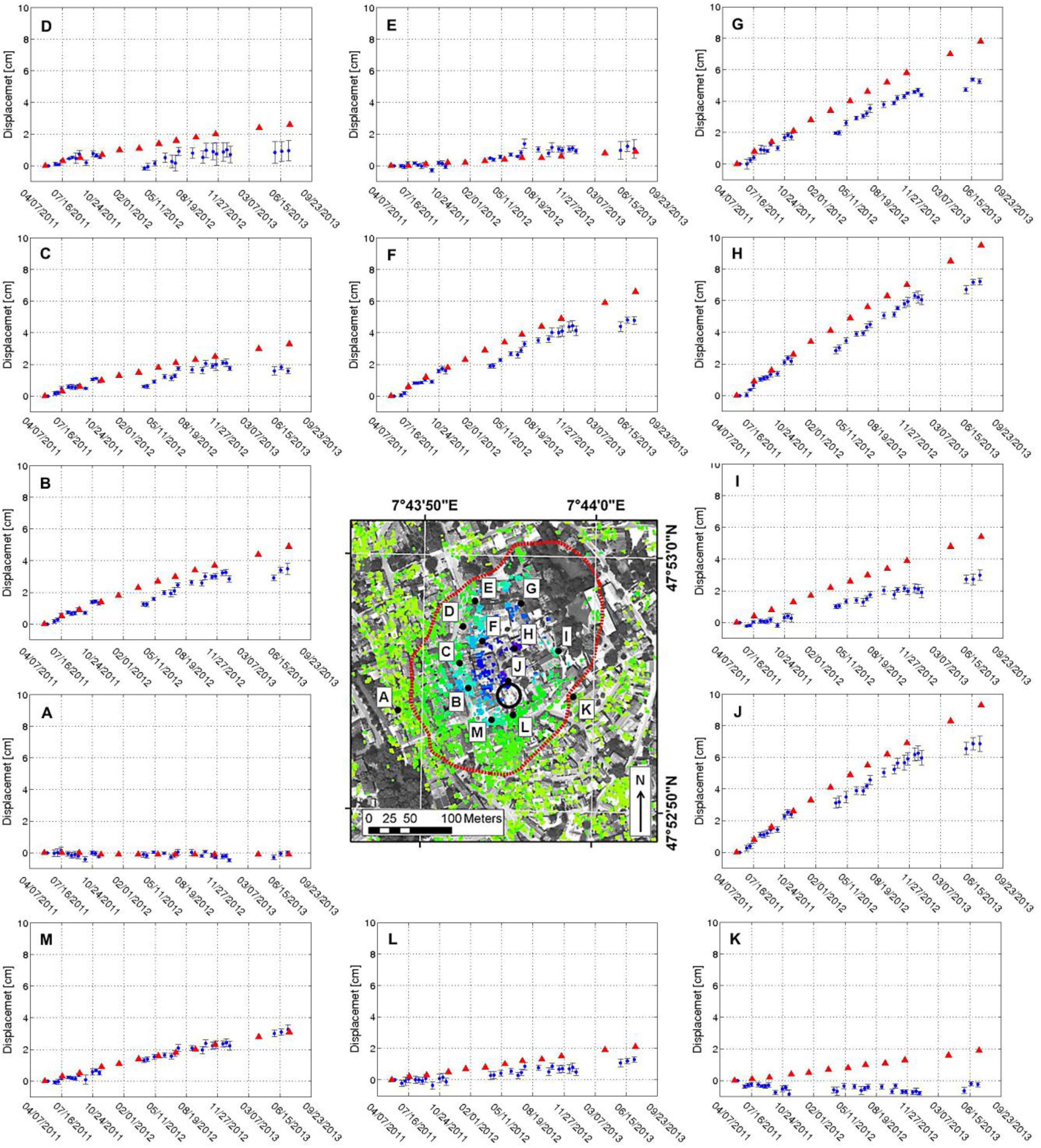
4. Results
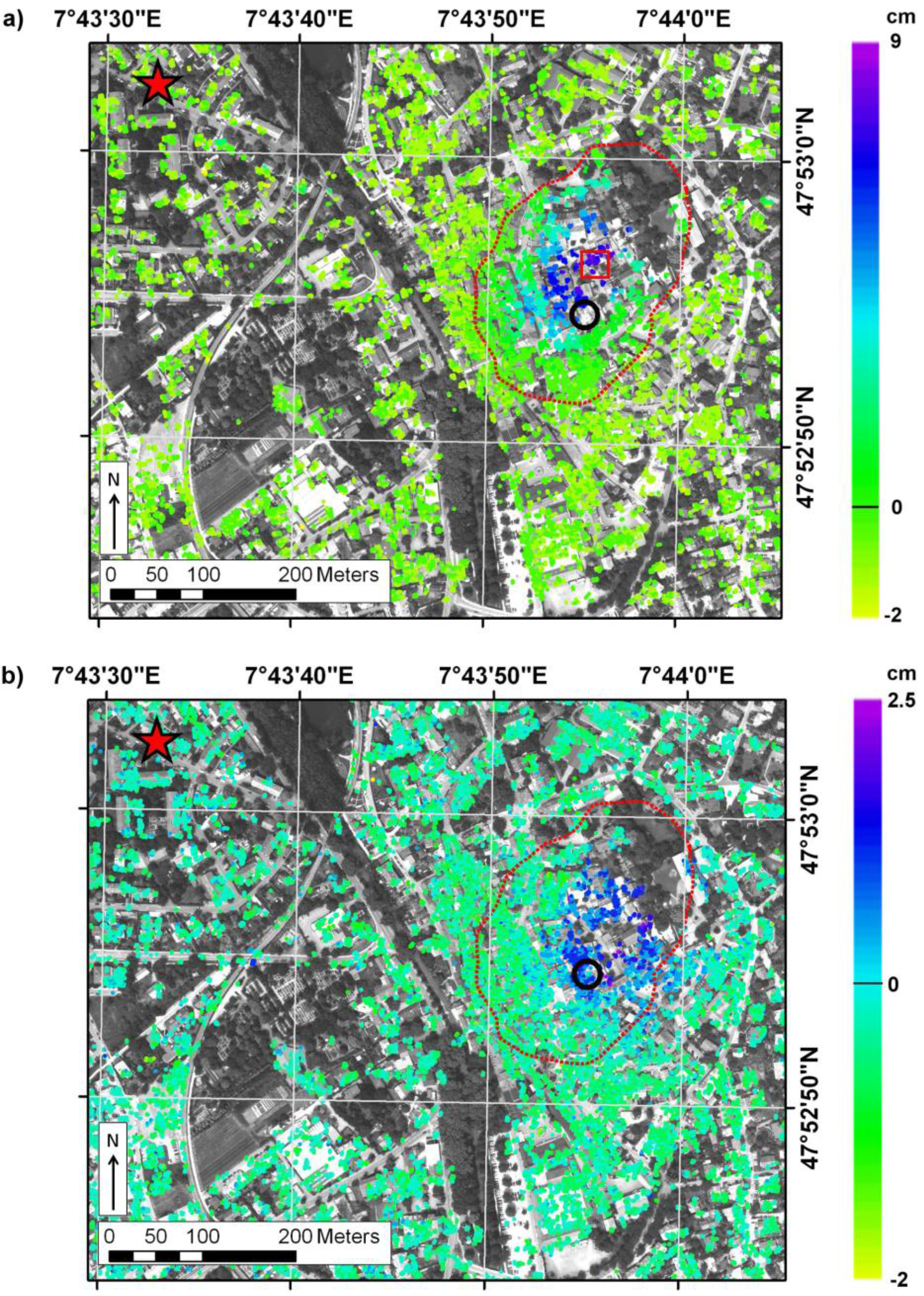
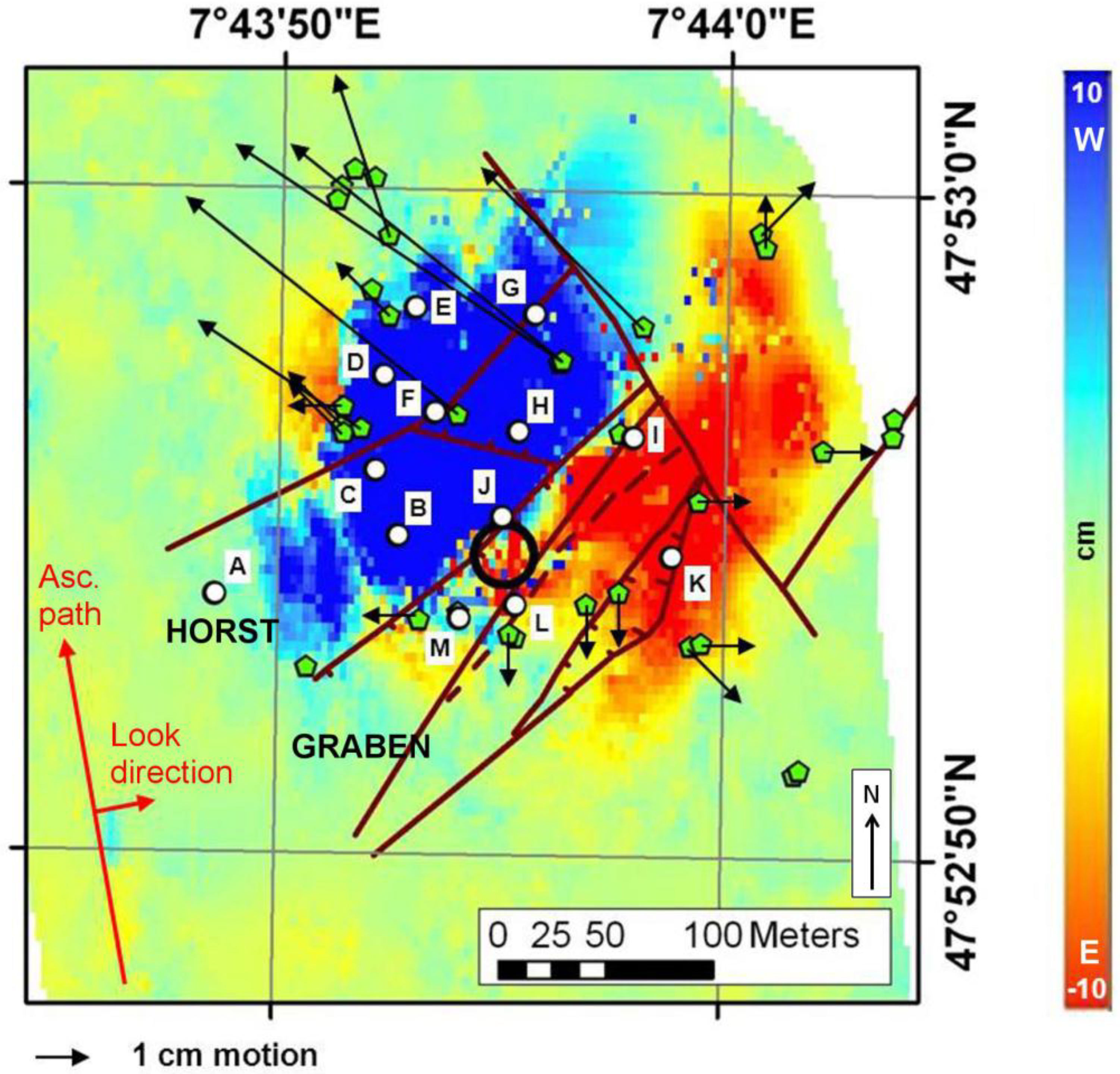
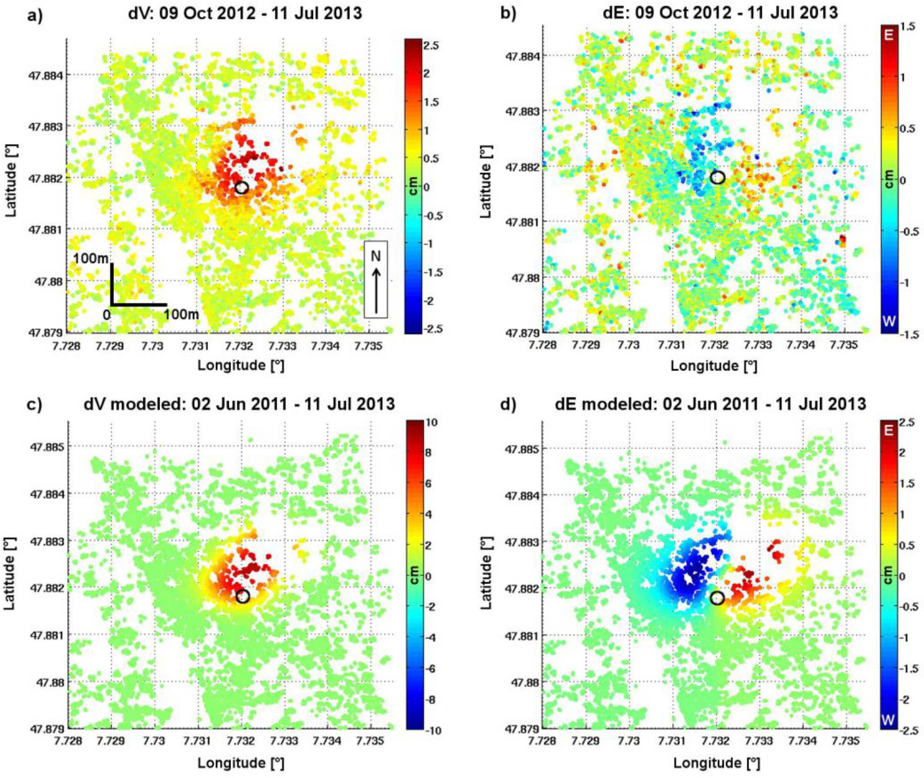
4.1. InSAR Derived Motion
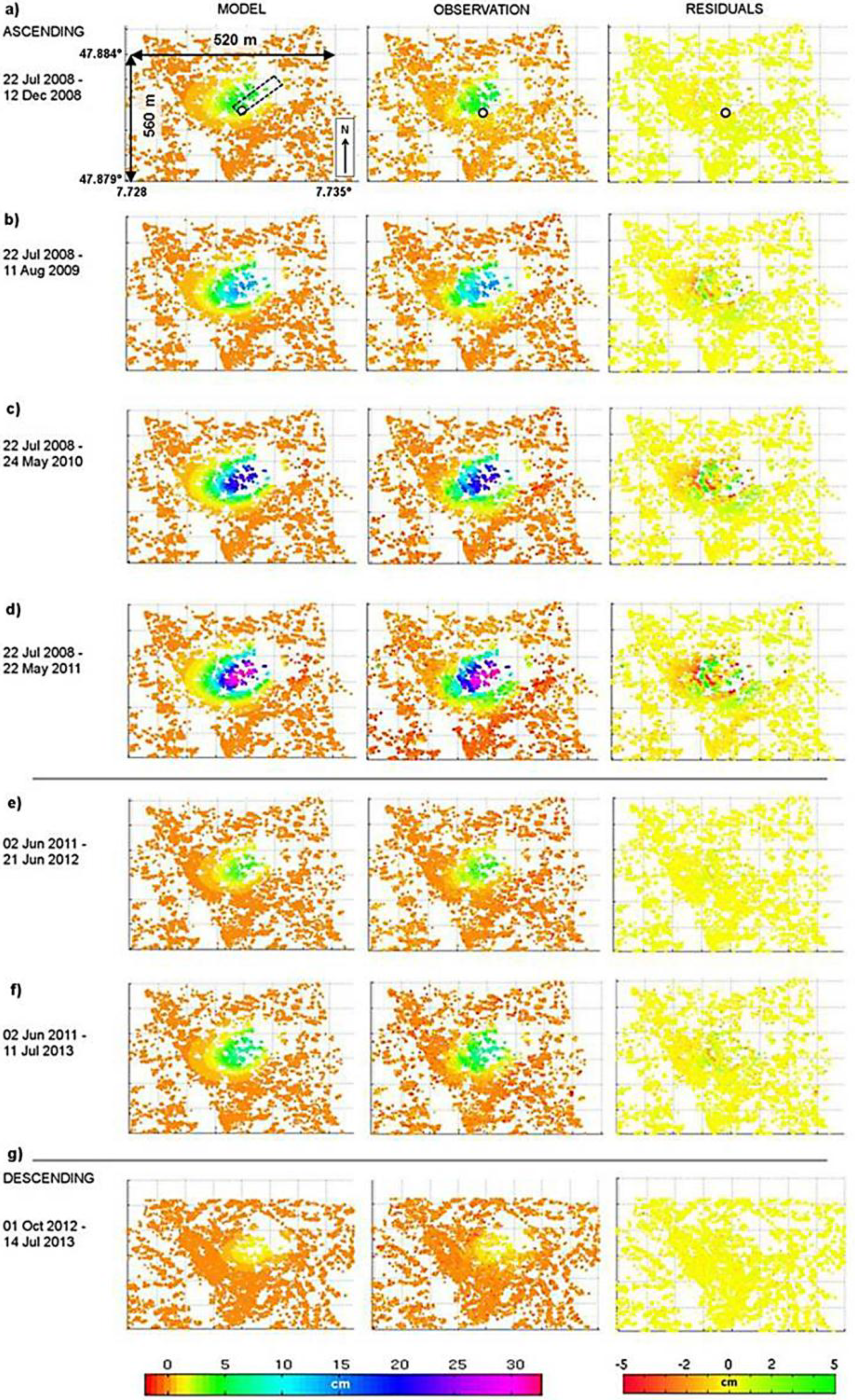
4.2. Modeled Source Parameters


| Source Parameters | Ascending | Descending | |||||
|---|---|---|---|---|---|---|---|
| Jul 2008–Dec 2008 | Jul 2008–Aug 2009 | Jul 2008–May 2010 | Jul 2008–May 2011 | Jun 2011–Jun 2012 | Jun 2011–Jul 2013 | Oct 2012–Jul 2013 | |
| Length (m) | 175 ± 27 | 173 ± 15 | 171 ± 14 | 164 ± 12 | 171 ± 32 | 174 ± 24 | 167 ± 26 |
| Width (m) | 51 ± 8 | 65 ± 9 | 69 ± 2 | 71 | 64 ± 14 | 64 ± 12 | 101 ± 12 |
| Depth (m) | 63 ± 12 | 49 | 46 | 45 | 51 ± 4 | 52 ± 2 | 48 ± 23 |
| Dip (°) | −1 ± 4 | 0 ± 3 | 0 ± 2 | 0 ± 2 | 0 ± 5 | 0 ± 4 | 0 ± 6 |
| Strike (°) | 39 ± 9 | 38 ± 5 | 39 ± 5 | 38 ± 4 | 34 ± 10 | 33 ± 8 | 41 ± 12 |
| Opening (cm) | 15 | 28 | 42 | 56 | 8 | 15 | 2 |
| Opening rate (cm/month) | 3 | 2.6 | 1.9 | 1.7 | 0.7 | 0.6 | 0.2 |
| Source Parameters | Oct 2012–Jul 2013 |
|---|---|
| Length (m) | 177 ± 19 |
| Width (m) | 69 ± 15 |
| Depth (m) | 89 ± 9 |
| Dip (°) | 0 ± 1 |
| Strike (°) | 37 ± 5 |
| Opening (cm) | 6 |
| Opening Rate (cm/month) | 0.7 |

5. Discussion
5.1. Uplift Deceleration in Response to Counteractions
| Statistics | 22 July 2008–31 July 2009 | 31 July 2009–18 July 2010 | 18 July 2010–22 May 2011 | 5 July 2011–13 July 2012 | 13 July 2012–11 July 2013 |
|---|---|---|---|---|---|
| Minimum (cm) | 12.8 | 10.3 | 6.4 | 3.7 | 2.3 |
| Maximum (cm) | 14.2 | 11.7 | 7.8 | 4.8 | 3.5 |
| Mean (cm) | 13.7 | 11.1 | 6.9 | 4.01 | 3 |
| Median (cm) | 13.8 | 11 | 6.8 | 4.1 | 3 |
| Standard deviation (cm) | 0.3 | 0.3 | 0.3 | 0.2 | 0.3 |
5.2. Horizontal Displacement Estimation
5.2.1. Evidence from Comparing Time Series of SBAS and Leveling Measurements


5.2.2. Evidence from Ascending and Descending Data Processing

5.3. Model Evaluation

6. Conclusions
Acknowledgments
Author Contributions
Conflicts of Interest
References
- Geologische Untersuchungen von Baugrundhebungen im Bereich des Erdwärmesondenfeldes beim Rathaus in der historischen Altstadt von Staufen i. Br; LGRB Landesamt für Geologie, Bergbau und Rohstoffe Baden-Württemberg: Regierungspräsidium Freiburg, Germany, 2010.
- Zweiter Sachstandsbericht zu den seit dem 01.03.2010 erfolgten Untersuchungen im Bereich des Erdwärmesondenfeldes beim Rathaus in der historischen Altstadt von Staufen i. Br; LGRB Landesamt für Geologie, Bergbau und Rohstoffe Baden-Württemberg: Regierungspräsidium Freiburg, Germany, 2012.
- Lubitz, C.; Motagh, M.; Wetzel, H.-U.; Kaufmann, H. Remarkable urban uplift in Staufen im Breisgau, Germany: Observations from TerraSAR-X InSAR and leveling from 2008 to 2011. Remote Sens. 2013, 5, 3082–3100. [Google Scholar]
- Sass, I.; Burbaum, U. Damage to the historic town of Staufen (Germany) caused by geothermal drillings through anhydrite-bearing formations. Acta Carsologica 2010, 39, 233–245. [Google Scholar]
- Sass, I.; Burbaum, U. Geothermische Bohrungen in Staufen im Breisgau: Schadensursachen und Perspektiven. Geotechnik 2012, 35, 198–205. [Google Scholar]
- Frühere Schlossberg-Wäscherei wurde abgerissen. Available online: www.staufen.de/aktuelles-nachrichten/hebungsrisse/fruehere-schlossberg-waescherei-wurde-abgerissen-~164934/ (accessed on 4 December 2013).
- Okada, Y. Surface deformation due to shear and tensile faults in a half-space. Bull. Seismol. Soc. Am. 1985, 75, 1135–1154. [Google Scholar]
- Hebungsrisse: Runder Tisch vom 14.01.2013. Available online: www.staufen.de/aktuelles-nachrichten/hebungsrisse/protokolle-runder-tisch/hebungsrisse-runder-tisch-~164899/ (accessed on 25 October 2013).
- Hooper, A. A multi-temporal InSAR method incorporating both persistent scatterer and small baseline approaches. Geophys. Res. Lett. 2008, 35. [Google Scholar] [CrossRef]
- Kampes, B.M.; Hanssen, R.F.; Perski, Z. Radar interferometry with public domain tools. In Proceedings of The Third International Workshop on ERS SAR Interferometry, Frascati, Italy, 1–5 December 2003.
- Berardino, P.; Fornaro, G.; Lanari, R.; Sansosti, E. A new algorithm for surface deformation monitoring based on small baseline differential SAR interferograms. IEEE Trans. Geosci. Remote Sens. 2002, 40, 2375–2383. [Google Scholar]
- Lanari, R.; Mora, O.; Manunta, M.; Mallorquí, J.J.; Berardino, P.; Sansosti, E. A small-baseline approach for investigating deformations on full-resolution differential SAR interferograms. IEEE Trans. Geosci. Remote Sens. 2004, 42, 1377–1386. [Google Scholar]
- Anderssohn, J.; Motagh, M.; Walter, T.R.; Rosenau, M.; Kaufmann, H.; Oncken, O. Surface deformation time series and source modeling for a volcanic complex system based on satellite wide swath and image mode interferometry: The Lazufre system, central Andes. Remote Sens. Environ. 2009, 113, 2062–2075. [Google Scholar]
- Motagh, M.; Wang, R.; Walter, T.R.; Bürgmann, R.; Fielding, E.; Anderssohn, J.; Zschau, J. Coseismic slip model of the 2007 August Pisco earthquake (Peru) as constrained by Wide Swath radar observations. Geophys. J. Int. 2008, 174, 842–848. [Google Scholar]
- Stramondo, S.; Moro, M.; Tolomei, C.; Cinti, F.R.; Doumaz, F. InSAR surface displacement field and fault modelling for the 2003 Bam earthquake (southeastern Iran). J. Geodyn. 2005, 40, 347–353. [Google Scholar]
- Pedersen, R.; Jónsson, S.; Árnadóttir, T.; Sigmundsson, F.; Feigl, K.L. Fault slip distribution of two June 2000 Mw 6.5 earthquakes in South Iceland estimated from joint inversion of InSAR and GPS measurements. Earth Planet. Sci. Lett. 2003, 213, 487–502. [Google Scholar]
- Sambridge, M.; Mosegaard, K. Monte carlo methods in geophysical inverse problems. Rev. Geophys. 40. [CrossRef]
- Faegh-Lashgary, P.; Motagh, M.; Sharifi, M.-A.; Saradjian, M.-R. Source parameters of the September 10, 2008 Qeshem Earthquake in Iran inferred from the bayesian inversion of Envisat and ALOS InSAR observations. In VII Hotine-Marussi Symposium on Mathematical Geodesy, International Association of Geodesy Symposia; Sneeuw, N., Novák, P., Crespi, M., Sansò, F., Eds.; Springer-Verlag: Berlin/Heidelberg, Germany, 2012; Volume 137, pp. 319–325. [Google Scholar]
- Lee, F.T.; Abel, J.F., Jr. Subsidence from underground mining: Environmental analysis and planning considerations. In Publications of the Geological Survey, 1983; U.S. Geological Survey: Reston, VA, USA, 1983; p. 28. [Google Scholar]
- Whittaker, B.N.; Reddish, D.J. Subsidence–Occurrence, Prediction and Control; Elsevier Science Publishers B.V.: Amsterdam, The Netherlands, 1989. [Google Scholar]
- Yao, X.L.; Whittaker, B.N.; Reddish, D.J. Influence of overburden mass behavioural properties on subsidence limit characteristics. Min. Sci. Technol. 1991, 13, 167–173. [Google Scholar]
- Singh, K.B.; Singh, T.N. Ground movements over longwall workings in the Kamptee coalfield, India. Eng. Geol. 1998, 50, 125–139. [Google Scholar]
- Pritchard, M.E.; Simons, M. An InSAR-based survey of volcano deformation in the central Andes. Geochem. Geophys. Geosystems 2007, 5. [Google Scholar] [CrossRef]
- Hernandez-Marin, M.; Burbey, T.J. The role of faulting on surface deformation patterns from pumping-induced groundwater flow (Las Vegas Valley, USA). Hydrogeol. J. 2009, 17, 1859–1875. [Google Scholar]
- Hanssen, R.F. Radar Interferometry—Data Interpretation and Error Analysis, 2nd ed.; van der Meer, F., Ed.; Kluwer Academic Publishers: Dordrecht, The Netherlands, 2001. [Google Scholar]
- Samieie-Esfahany, S.; Hanssen, R.F.; van Thienen-Visser, K.; Muntendam-Bos, A. On the effect of horizontal deformation on InSAR subsidence estimates. In Proceedings of The Fringe 2009 Workshop, Frascati, Italy, 30 November–4 December 2009.
- Cayol, V.; Cornet, F.H. Effects of topography on the interpretation of the deformation field of prominent volcanoes—Application to Etna. Geophys. Res. Lett. 1998, 25, 1979–1982. [Google Scholar]
© 2014 by the authors; licensee MDPI, Basel, Switzerland. This article is an open access article distributed under the terms and conditions of the Creative Commons Attribution license (http://creativecommons.org/licenses/by/4.0/).
Share and Cite
Lubitz, C.; Motagh, M.; Kaufmann, H. Ground Surface Response to Geothermal Drilling and the Following Counteractions in Staufen im Breisgau (Germany) Investigated by TerraSAR-X Time Series Analysis and Geophysical Modeling. Remote Sens. 2014, 6, 10571-10592. https://doi.org/10.3390/rs61110571
Lubitz C, Motagh M, Kaufmann H. Ground Surface Response to Geothermal Drilling and the Following Counteractions in Staufen im Breisgau (Germany) Investigated by TerraSAR-X Time Series Analysis and Geophysical Modeling. Remote Sensing. 2014; 6(11):10571-10592. https://doi.org/10.3390/rs61110571
Chicago/Turabian StyleLubitz, Christin, Mahdi Motagh, and Hermann Kaufmann. 2014. "Ground Surface Response to Geothermal Drilling and the Following Counteractions in Staufen im Breisgau (Germany) Investigated by TerraSAR-X Time Series Analysis and Geophysical Modeling" Remote Sensing 6, no. 11: 10571-10592. https://doi.org/10.3390/rs61110571