Temporal and Spectral Optimization of Vegetation Indices for Estimating Grain Nitrogen Uptake and Late-Seasonal Nitrogen Traits in Wheat


Chair of Plant Nutrition, Technical University of Munich, 85354 Freising, Germany
*
Author to whom correspondence should be addressed.
Sensors 2019, 19(21), 4640; https://doi.org/10.3390/s19214640
Submission received: 9 September 2019
/
Revised: 20 October 2019
/
Accepted: 22 October 2019
/
Published: 25 October 2019
(This article belongs to the Section Remote Sensors)
Abstract
:Grain nitrogen (N) uptake (GNup) in winter wheat (Triticum aestivum L.) is influenced by multiple components at the plant organ level and by pre- and post-flowering N uptake (Nup). Although spectral proximal high-throughput sensing is promising for field phenotyping, it was rarely evaluated for such N traits. Hence, 48 spectral vegetation indices (SVIs) were evaluated on 10 measurement days for the estimation of 34 N traits in four data subsets, representing the variation generated by six high-yielding cultivars, two N fertilization levels (N), two sowing dates (SD), and two fungicide (F) intensities. Close linear relationships (p < 0.001) were found for GNup both in response to cultivar differences (Cv; R2 = 0.52) and other agronomic treatments (R2 = 0.67 for Cv*F*N, R2 = 0.53 for Cv*SD*N and R2 = 0.57 for the combined treatments), notably during milk ripeness. Especially near-infrared (NIR)/red edge SVIs, such as the NDRE_770_750, outperformed NIR/visible light (VIS) indices. Index rankings and seasonal R2 values were similar for total Nup, while the N harvest index, which expresses the partitioning to the grain, was moderately estimated only during dough ripeness, primarily from indices detecting contrasting senescence between different fungicide intensities. Senescence-sensitive indices, including R787_R765 and TRCARI_OSAVI, performed best for N translocation efficiency and some organ-level N traits at maturity. Even though grain N concentration was best assessed by the red edge inflection point (REIP), the blue/green index (BGI) was more suited for leaf-level N traits at anthesis. When SVIs were quantitatively ranked by data subsets, a better agreement was found for GNup, total Nup, and grain N concentration than for several contributing N traits. The results suggest (i) a good general potential for estimating GNup and total Nup by (ii) red edge indices best used (iii) during milk and early dough ripeness. The estimation of contributing N traits differs according to the agronomic treatment.
1. Introduction
Although plant breeding in winter wheat traditionally focuses on the maximization of grain yield (GY) at sufficient grain N concentration (GNC), the efficient use of nitrogen (N) for grain N uptake (GNup) is gaining more attention for reducing N surplus and increasing the effective N uptake efficiency (NupEff) of a cropping system [1,2]. Similar to GY, GNup strongly depends on the environment. Moreover, interactions among agronomic treatment factors such as sowing date, fungicide intensity, N fertilization, and genotypes are relevant [3,4,5,6,7,8,9,10,11,12]. Expensive field trials have to be conducted for assessing the optimum treatment levels in different cropping environments, both for the selection of N-efficient genotypes in plant breeding, and for optimizing agronomic treatment factors [13].
However, being costly and time-consuming, the determination of plant traits is often restricted to only a few traits, such as GY and yield components, or it relies on visual scoring, which is subjective and expensive [14]. Non-destructive high-throughput proximal sensing has been developed for optimizing N management in the vegetative phase, and has become an approved tool in precision farming [15]. However, the generative phase is also important for maximizing GNup [16]. Post-anthesis N uptake (PANup) and N translocation (NT) respond to agronomic treatments, differ among cultivars, and influence total N uptake (Nup) as well as its partitioning to the grain [12,17]. Although vegetative Nup is primarily allocated to leaves, the organs which are more visible to spectral sensors [18], substantial amounts of N are allocated to stems and spikes until anthesis [19], and are predominantly translocated to the grain during the influence of senescence [20,21].
The spectral in-season estimation of GY has been addressed as a tool in plant phenotyping in various studies [22,23,24,25]. However, the estimation of GNup was evaluated less frequently, not to mention the contributing traits at the organ-level or seasonal dynamics. Compared from simulated band configuration, GNup was generally well estimated from red edge (RE) indices at milk ripeness, but also stem elongation was well suited in the presence of different N fertilization levels [26]. For breeding lines, Pavuluri et al. [27] reported better estimations of GNup and NupEff than those of GY, and better estimations for multi-year data than those for individual years. Moreover, correlations were closer under reduced N fertilization, ascribed to less saturation in thinner canopies. Using RE-based spectral vegetation indices (SVIs) in winter wheat, Frels et al. [28] complemented the estimation of GNup with that of PANup, total Nup, and the N harvest index (NHI). The estimation of PANup and NHI differed more between years than that of NupEff and GNup. They recommended the RE Maccioni index and identified the early grain filling stage as the most promising. Pavuluri et al. [27] suggested the related simple ratio index R780/R740 [29] and recommended the heading stage, followed by booting, stem elongation, and grain filling. For organ-level Nup in spring barley, Barmeier and Schmidhalter [18] reported better correlations for leaf blades and culms than for spikes and leaf sheaths.
Nonetheless, knowledge on the use of spectral methods for GNup and its contributing traits remains scarce, notably concerning high-yielding European conditions, as well as the impact of different agronomic treatments, compared to the use for estimating genotypic differences. Therefore, this study assesses the spectral estimation of the N traits previously compared in [12]. These traits include plant- and organ-level N concentration (NC) and Nup and traits related to NT and N allocation as a function of two levels of N fertilization, fungicide intensity and sowing dates for six winter wheat cultivars. We evaluated the (i) estimation potential by trait, (ii) identified suitable vegetation indices and (iii) optimum growth stages, and (iv) compared the differences in (i–iii) by underlying treatments. Although based on hyperspectral phenotyping, the results could be transferred to the use of simpler multispectral methods.
2. Materials and Methods
2.1. Experiment and Plant Sampling
The field trial, conducted as a split-split-plot design, comprised control (Cont)/reduced fungicide (RF)/early sowing (sowing date 1: SD1) on the main plot (MP), N level (N) on the sub-plot (SP), and cultivar (Cv) on the sub-sub-plot. It was conducted during the 2016/2017 growing season in southeastern Germany (48.406° N, 11.692° E) on homogeneous Cambisol of silty clay loam. The average annual temperature is approximately 8 °C and the annual precipitation approximately 800 mm. The previous crop grass-clover resulted in high soil mineral N content of 83 and 92 kg N ha−1 in SD1 and 69 and 87 kg N ha−1 in Cont in autumn and after winter, respectively. Six morphologically and phenologically differing cultivars (cv. Impression, JB Asano, Kerubino, Hybred, Hyland, Hystar) of winter wheat (Triticum aestivum L.) were drilled at 350 kernels m−2 in plots of 1.5 m in width and 6.4 m in length. Cultivars differed in anthesis date by up to six days, in plant height by 11 cm, in average plant density from 571–728 spikes per m2, and reacted differently to the agronomic treatments [12]. The sowing date was September 28 for SD1 and October 23 for Cont and RF. Within each MP, each cultivar was treated in two N levels, with N1 corresponding to 60 kg N ha−1 and N2 to 120 kg N ha−1, applied as ammonium nitrate in two equally split doses at tillering and stem elongation, respectively. The trial comprised four replicates for each factor combination (MP*N*Cv). Foliar fungicide was applied twice in Cont and SD1 plots, but not in RF plots. Fungicide was effective against the dominant pathogens Erysiphe graminis, Septoria tritici, and Puccinia striiformis, which showed only moderate incident in RF due to favorable weather conditions [12]. Above-average temperature and global radiation in March, May, and June together with high soil N supply resulted in strong vegetative growth, whereas below-average precipitation in May and June resulted in mild drought stress and accelerated senescence in some cultivars. Refer to [12] for details on the field trials, weather conditions, and treatment effects on the plant traits.
Biomass was sampled at anthesis (Zadok’s growth stage 65) and at physiological maturity (growth stage 95). For each genotype within each subplot, sampling dates were determined by visual scoring. In total 30 and 60 randomly selected shoots were cut per plot at the stem base at anthesis and maturity, respectively. Plant samples were manually separated into flag leaves, flag leaves–1 (second leaf from above), ‘other leaves’ (remaining leaves), culms including all leaf sheaths, and spikes. Plant samples were oven-dried at 50 °C for 2–4 days until no further weight loss was observed for subsequent determination of dry matter (DM) weight. After plant sampling at maturity, all plots were harvested (1–2 August 2017) using a combine harvester, to determine moisture-corrected grain yield (0%) for each plot. After grinding, the N concentration (NC) was determined by near-infrared spectroscopy (NIRS) using a FOSS NIRS 6500 (Foss, Silver Spring, MD, USA) and a Fourier-Transform -NIRS (Bruker, Billerica, MA, USA), whereas grains were analyzed as complete kernels. The calculation of ‘derived’ plant traits [20] comprised the N harvest index (NHI), post-anthesis N uptake (PANup), N translocation efficiency (NTEff), N translocation (NT), the contribution of PANup to total Nup (CPostNup), and the N uptake efficiency (NupEff), both at anthesis and at maturity. See [12] for details and Table S1 for a list of included traits.
2.2. Spectral Measurements and Data Preparation
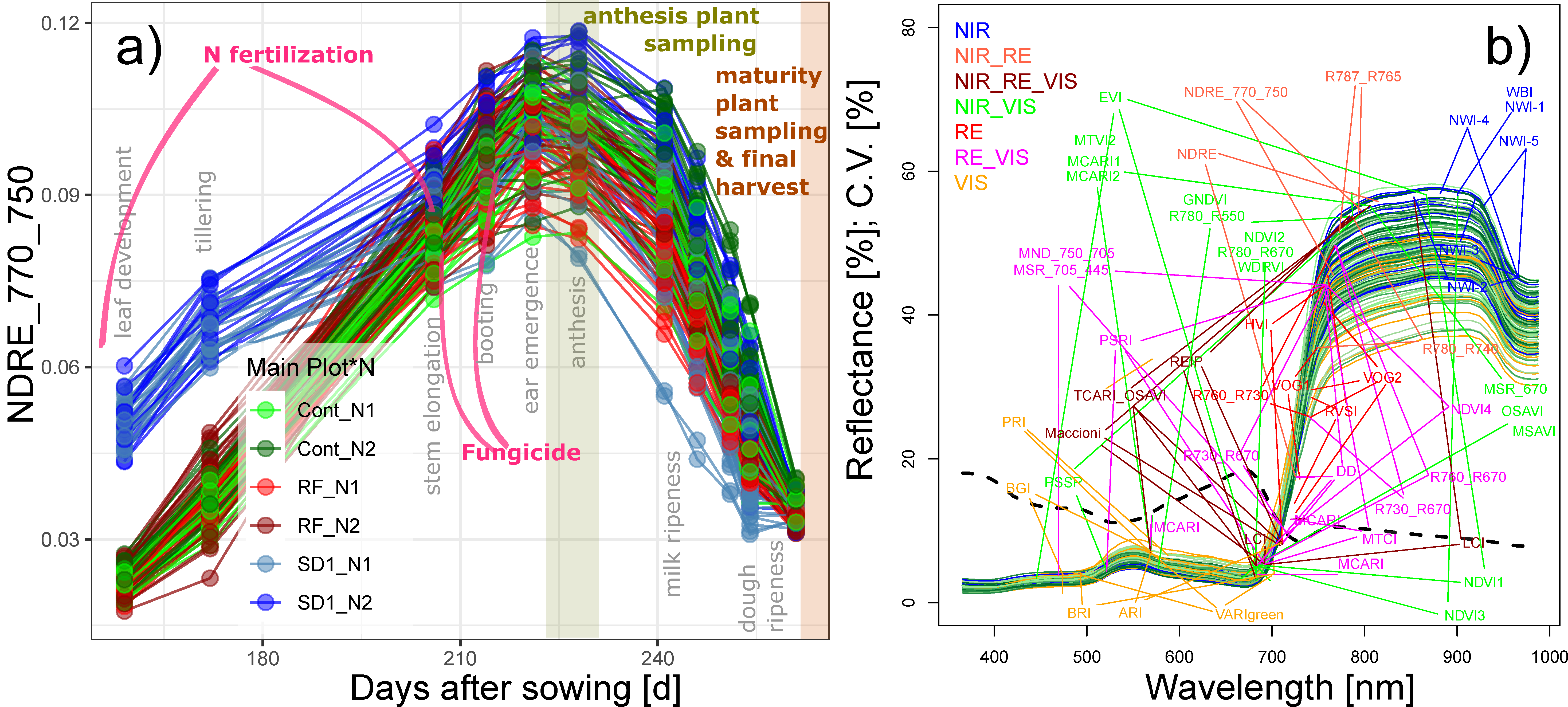
Spectral measurements were performed on 10 measurement days, covering all main growth stages from leaf development at the end of March until soft dough ripeness in July (Figure 1a; Table 1), using the mobile sensor platform PhenoTrac 4 [18]. It was equipped with a hyperspectral bidirectional passive point sensor spectrometer (tec5, Oberursel, Germany), measuring at a nominal resolution of 3.3 nm between 300 and 1000 nm at a frequency of 5 Hz. Plot boundaries were excluded and the distance to the canopy was ≈80 cm. The driving speed was ≈5 km h−1, resulting in a sampling distance of ≈28 cm at the top of the canopy and typically 15–20 registered spectra per target plot area, which allowed gapless sampling in a longitudinal direction in the middle of the plots. The resulting measurement strip was approximately 30–35 cm wide. Measurements were localized via a real-time kinematic global positioning system (RTK-GPS; Trimble, Sunnyvale, CA, USA). Based on polygons drawn to the core target plot area, the spectra were averaged to the plot level using custom-made LabView applications. Refer to Figure S1 for an example of the trial measurements. Spectra were smoothed using a 5 band moving average filter [30] for removing spectral noise. A total of 48 spectral vegetation indices (SVI) were calculated based on a literature review of related previous studies (Table 1). The SVIs were grouped by the included spectral range (visible light (VIS), red edge (RE), and near-infrared (NIR)), with VIS < 700 nm, ‘extended’ RE 700–765 nm, and NIR > 765 nm (Table 2; Figure 1b). In order to include SVIs with a NIR or RE band closer to the RE than that of the normalized difference vegetation index (NDVI; NIR = 780 nm), the upper boundary of the RE was higher than the common definition since the reflection still increased in region until approximately 770 nm.
2.3. Statistical Analysis
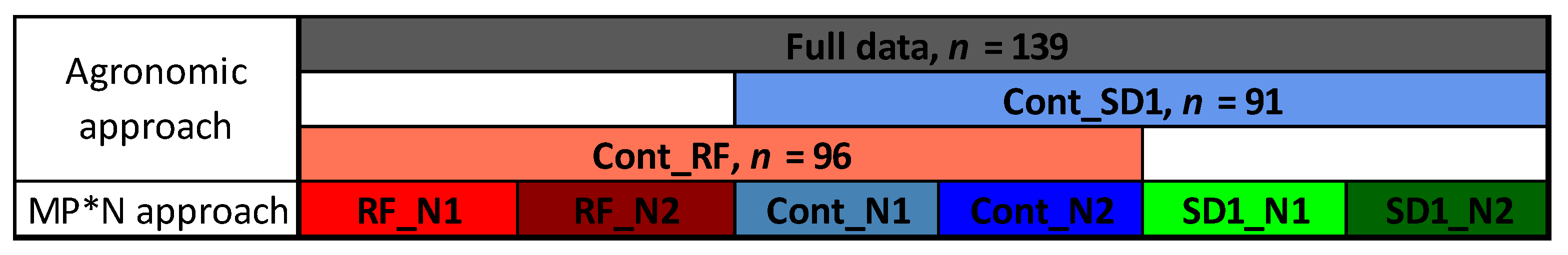
SVIs were tested in simple linear regression analysis with the N traits for each sampling date, using the lm-function in R 3.4 (R Core Team, 2017). Relationships were compared by coefficient of determination (R2) and the root mean square error (RMSE) derived from the deviations between fitted and measured values. The relationships were compared for (i) the full data, (ii) across the combined Cont and SD1 data (Cont_SD1), (iii) across the combined Cont and RF data (Cont_RF), and (iv) within the six main plot*N level (MP*N) combinations (Figure 2) to assess the influence of the underlying treatments on the trait estimation. The MP*N blocks were considered as possible trial environments. Therefore, the results of these blocks were averaged and compared for the aggregated, averaged results. This approach can simulate conditions for phenotyping genotypic variation as relevant for plant breeding, whereas (i–iii) are referred to as ‘agronomic’ conditions. The relationships were compared with respect to estimation potential by trait, index ranking, and optimum measurement stages.
The indices were quantitatively ranked by their normalized performance for each trait in each dataset in order to overcome the influence of differing growing conditions as well as the date-specific index ranking. Therefore, within each of the three ‘agronomic’ datasets and the MP*N data, the across-date mean and maximum coefficients of determination (R2) of each index/trait combination were normalized to the trait-specific average mean and maximum R2 from all SVIs. In order to achieve a more robust ranking across underlying treatments, both the within-dataset mean and maximum rankings were summed up across the three ‘agronomic’ datasets. Consequently, the mean- and maximum-based rankings were combined through summing up both rankings (i) for the agronomic approach and (ii) for the MP*N approach. Considering a selection of indices robust towards date-specific suitability as more important, the mean-based ranking was double-weighted. These weighted mean/maximum-rank sums (WMMRS) were compared between the agronomic and the MP*N approach. WMMRS values were used for identifying one trait-specific optimum index from the ‘agronomic’ approach. A WMMRS < 9 indicates below-average and WMMRS > 9 indicates above-average index performance for a specific trait. The performance of this WMMRS-based best indices was compared over time both in the agronomic and the MP*N datasets. Additionally, the ‘agronomic’ rankings were compared to the WMMRS rankings of the MP*N approach by Spearman’s rank correlation coefficient.
In order to validate the initial index grouping based on the included spectral bands, the indices were grouped by a cluster analysis (Ward’s method) based on the coefficients of determination achieved for the studied traits.
3. Results
3.1. Optimized Date Selection by Plant Trait and Index
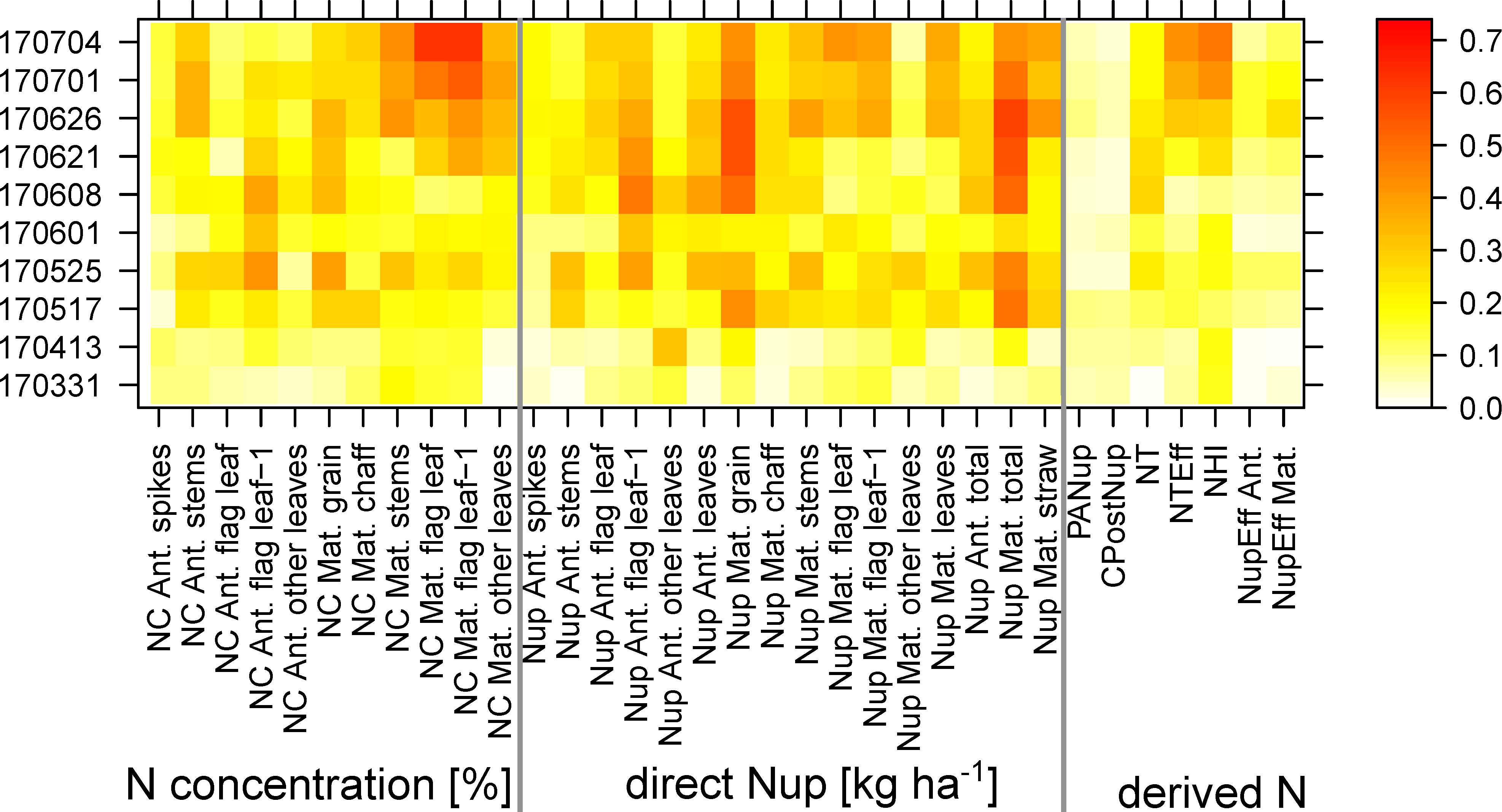
The maximum coefficients of determination (R2) were calculated for each trait*date combination from all SVIs as a measure of the potential to estimate the 34 plant traits (Figure 3 for full data; Figure S3 for other datasets). The relationships were low or moderate (R2 < 0.40) before anthesis (06/08) but increased during grain filling. For most traits, relationships increased at stem elongation and booting (05/17 and 05/25, R2 ≈ 0.20–0.50), but decreased sharply around ear emergence (06/01). Low relationships were found for post-anthesis Nup (PANup), the contribution of PANup to total Nup (CPostNup), and Nup efficiency (NupEff). Regarding the N concentration (NC) traits, NC of flag leaves and flag leaves–1 at maturity were best assessed, particularly on the late days (beginning of July, dough ripeness). Among direct Nup traits, relationships were closest for grain Nup (GNup) and total Nup. Similar seasonal maximum R2 patterns were found for the other ‘agronomic’ datasets, Cont_SD1 and Cont_RF (Figure S3). For several traits, higher R2 values were found in Cont_SD1 during stem elongation (05/17 and 05/25) and during grain filling, as well as for various traits in MP*N.
3.2. Optimized Index and Date Selection Considering the UnderlyingTtreatments
3.2.1. Grain Nup
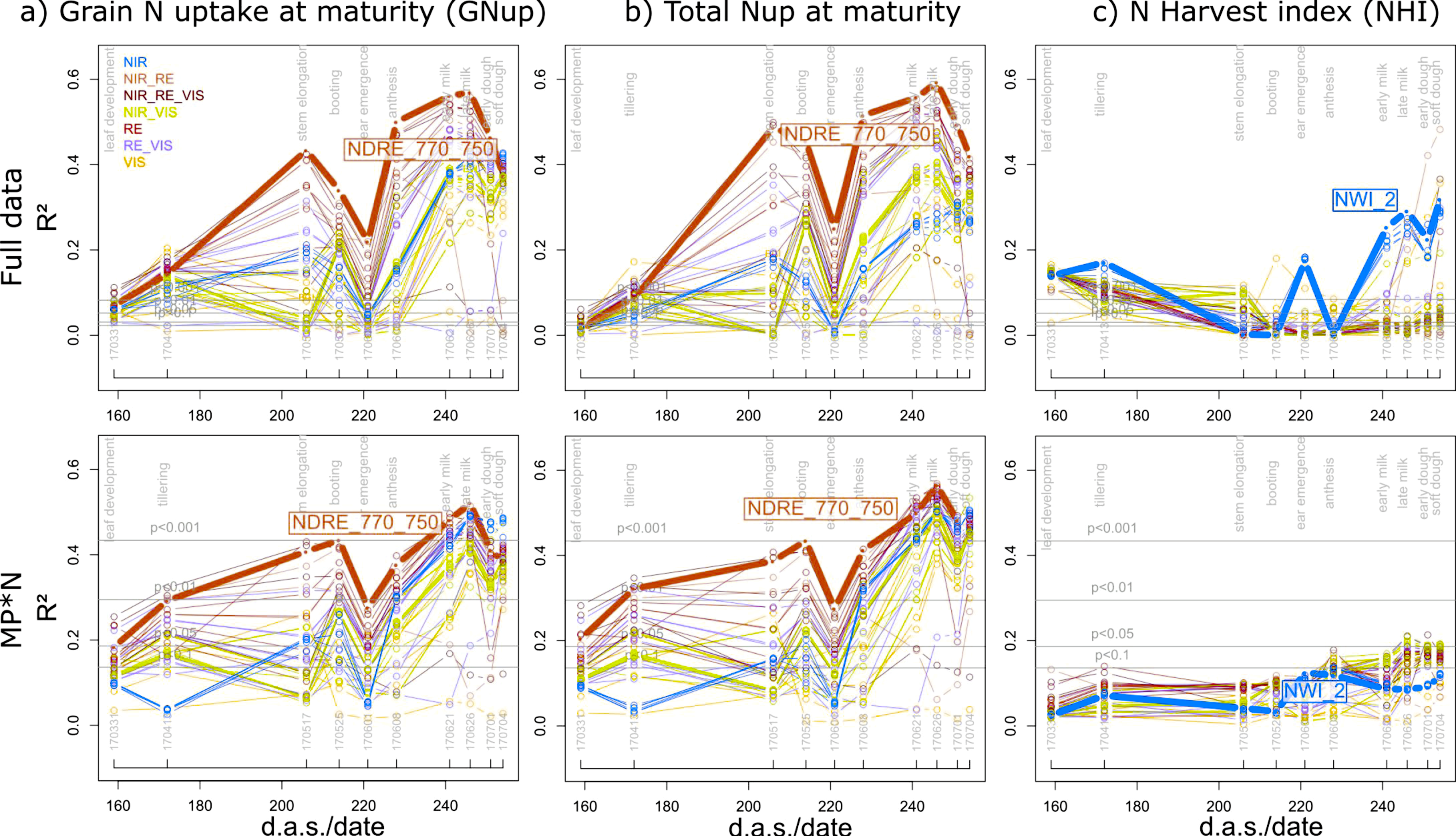
The estimation of GNup primarily relied on the assessment of its ‘accumulative component’ (i.e., total Nup at maturity), which was well assessed in all datasets with the best index based on the weighted mean/maximum-rank sums (WMMRS), NDRE_750_770, always during milk ripeness (06/26; R2 = 0.57–0.59 in the agronomic datasets and R2 = 0.35–0.78 in the individual MP*N datasets; Table 3). In contrast, moderate relationships were observed for the ‘partitioning component’, N harvest index (NHI), only for the full data, Cont_RF and some MP*N combinations (Figure 4; Table 3). The index rankings were similar for GNup and total Nup with NIR/RE and NIR/RE/VIS combinations ranking highest both in the agronomic and MP*N datasets (Figure 5). GNup was similarly detected seasonally as total Nup (Figure 5a,b), with similar R2 values and the highest precision observed as well as milk ripeness (RMSE = 9.7–16.7 kg N ha−1; Table 3; Figure 6). In contrast, the water band index NWI_2 ranked highest for NHI; however, the relationships were not consistent for the different datasets (Figure 5c; Figure 6c). Weaker relationships were found for total Nup and GNup at booting/grain filling than at stem elongation, and especially during grain filling.
3.2.2. Further Direct N traits
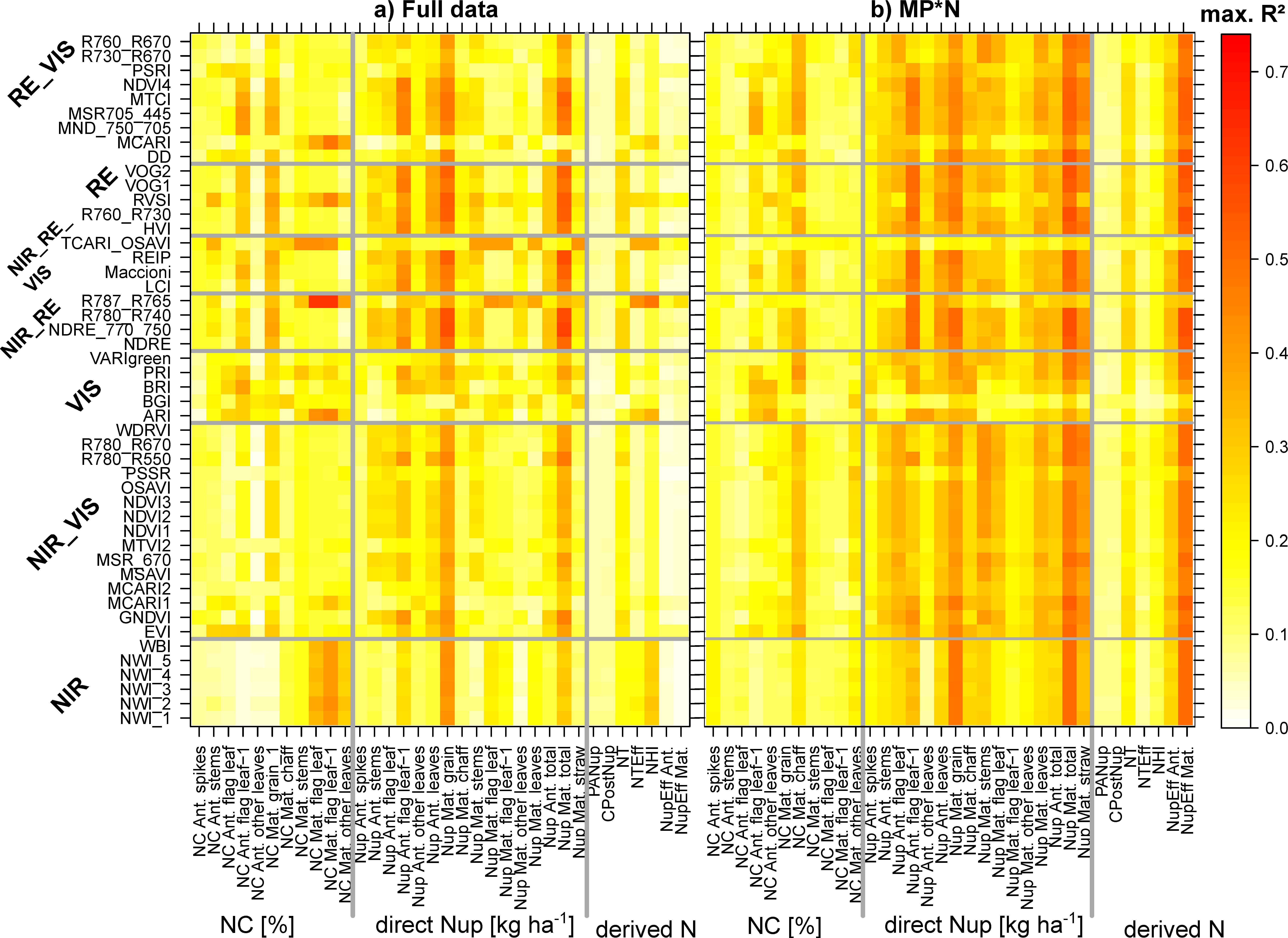
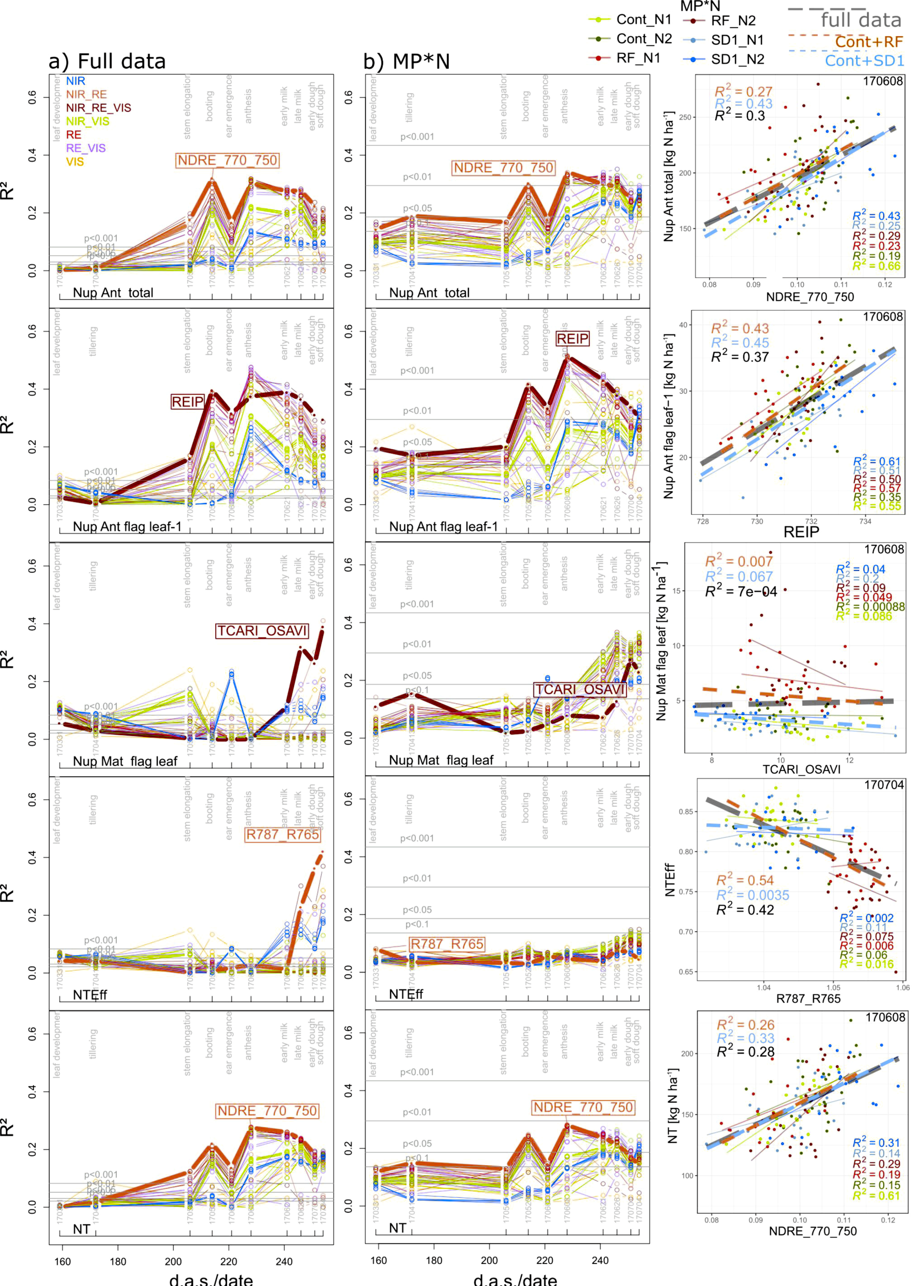
Index relationships for total Nup were weaker for anthesis Nup (Figure 7) than those for maturity Nup (Figure 5), but the index rankings were comparable. Moreover, the seasonal pattern was comparable for the full data, MP*N (Figure 7), and the other subsets (Figure S5 for total Nup). Both in the ‘agronomic’ and MP*N rankings, the index rankings for organ-level Nup were comparable with those for total Nup at anthesis and maturity (Figure 9). The Nup of spikes (at anthesis) and chaff (at maturity) was moderately detected by the WMMRS-based indices of the agronomic approach (R2 = 0.28–0.36) in Cont_SD1 and MP*N treatments (Table 3). Among the anthesis Nup traits, the Nup of flag leaves–1 was best detected (R2 from the REIP = 0.40–0.51 at anthesis; Table 3; Figure 7), followed by the Nup of flag leaves and stems (Table 3). In contrast, in spite of the good assessment of total Nup at maturity, only moderate relationships were found for straw Nup, primarily in the full data and in Cont_RF (R2 = 0.42 and 0.51, respectively), whereas the TCARI_OSAVI, the WMMRS-based best index in the agronomic approach, failed in the MP*N dataset (Table 3). The same index ranked highest for maturity Nup of stems, flag leaves, flag leaves–1, and the aggregated leaf Nup of all leaves, with moderate relationships (R2 = 0.37–0.46) in the full data and Cont_RF but weaker relationships in the MP*N data despite useful estimation of these traits from other indices (Figure 4).
3.2.3. Derived N Traits
Although the post-anthesis component PANup was not sufficiently assessed by any index, moderate relationships (R2 = 0.26–0.33; Table 3) were found for the N translocation (NT) from the same index which ranked highest for total Nup at anthesis, NDRE_770_750, always at anthesis (Figure 7). In contrast, good relationships were observed from a few indices including the WMMRS-index R787_765 at soft dough ripeness for N translocation efficiency (NTEff) only in the full data (R2 = 0.42) and Cont_RF (R2 = 0.54) (Table 3; Figure 7)—driven mainly by the lower NTEff in the RF plots compared with the Cont and SD1 plots. For the NupEff at maturity, which relates the Nup to the amount of fertilized N, the WMMRS-based best index R787_765 primarily captured the influence of both N levels irrespective of the main plot treatments in the agronomic datasets (Table 3).
3.2.4. N Concentration Traits
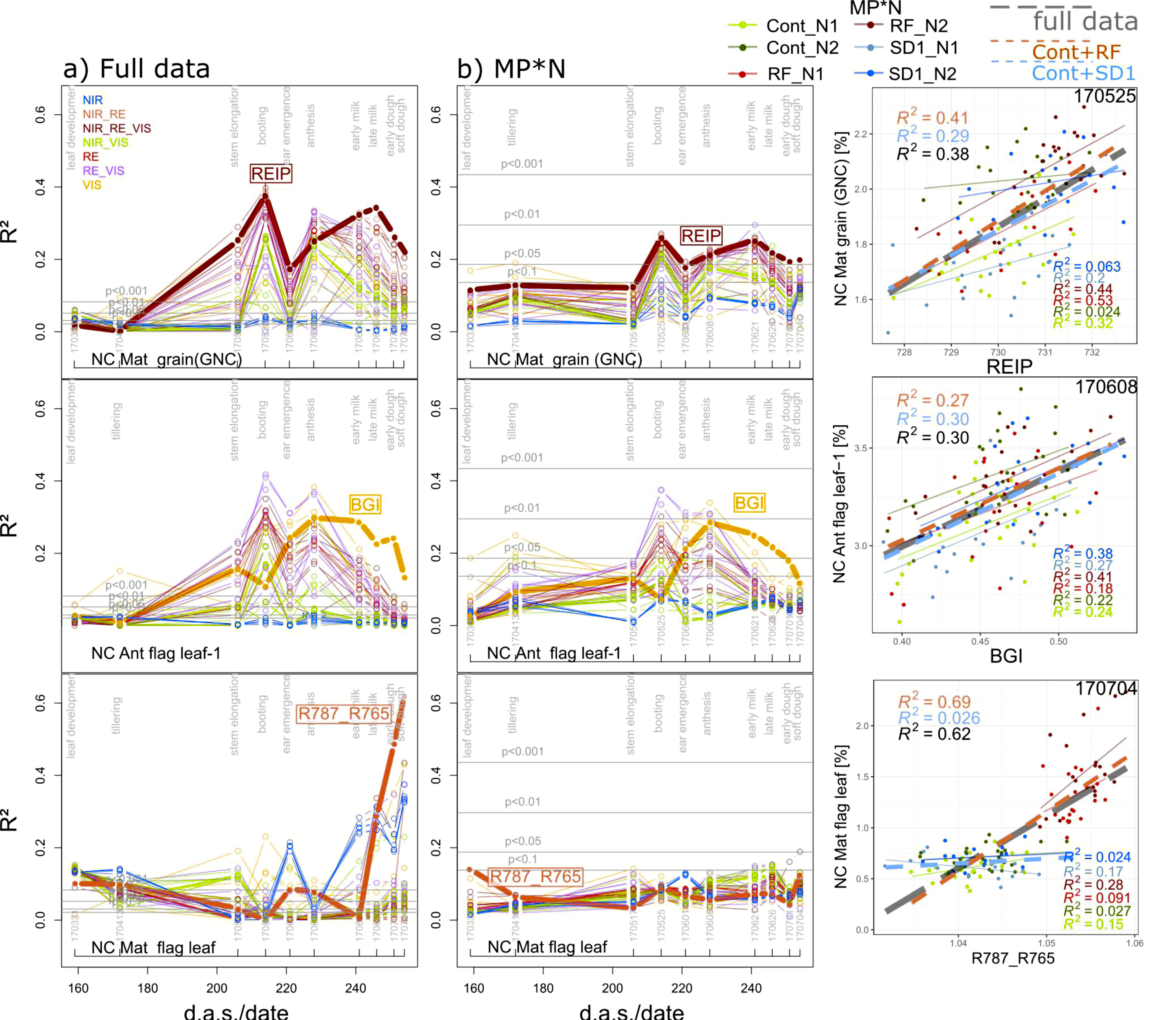
Organ-level N concentration (NC) was rarely detectable in the MP*N subsets with the exceptions of flag leaves–1, and ‘other leaves’ at anthesis (06/08; R2 = 0.28 and R2 = 0.29 from the BGI), and grain NC (GNC; 05/25; R2 = 0.26 from the REIP; Table 3). Driven by the positive effect of N fertilization on GNC in all main plots, relationships for GNC were closer in the agronomic datasets than in most MP*N except the RF-MPs (Table 3; Figure 8), with R2 peaks of the WMMRS-index REIP at booting and milk ripeness. Since reduced fungicide use in RF affected the release of leaf nitrogen, leaf NC at maturity was well detected in the full data and Cont_RF. However, this was based on few indices, including the R787_765 and the MCARI, and restricted to late growth stages.
3.3. Index Rankings According to Trait and Dataset
The WMMRS are depicted in Figure 9 for the combined rankings from the three ‘agronomic’ datasets (‘full data’, Cont_SD1, and Cont_RF; Figure 9a), as well as for the rankings from the MP*N data (Figure 9b). Owing to several upper outliers, values greater than 15 were colored with the same blue shading to allow for better comparisons of the other values. Only rankings for trait*index combinations that reached R2 values > 0.20 are shown. For the following traits, no index exceeded this threshold for the agronomic datasets: NC of spikes at anthesis as well as the derived N traits PANup, CPostNup, and NupEff at anthesis. The rankings for the NC traits were diffuse with several indices reaching high rank values for each few traits, but on a low absolute R2 level (Figure 4). For most Nup traits, a clear advantage of most RE-based indices is visible. The indices NDRE_770_750, R780_R740, REIP, R760_R730, Maccioni, and RVSI excelled through high-rank sums for most of the Nup traits in both rankings. R787_765 and TCARI_OSAVI reached higher rank sums (WMMRS >17) for maturity NC and Nup traits as well as NTEff and NHI in the agronomic ranking, but not in the MP*N ranking. In contrast, most NIR/VIS and VIS indices were not particularly useful for the assessment of any N trait. Overall, only a few indices reached ‘relevant’ relationships (R2 > 0.20) in both rankings for most NC traits and derived N traits. This was also the case for direct Nup traits in the agronomic approach, while index rankings differed less in the MP*N approach.
To compare the possibility of transferring the optimized index selection between datasets, the rankings of both matrices were correlated against each other (Table 4; Figure S6). Interestingly, rankings were substantially more stable (Spearman’s ρ > 0.84 ***) for all traits of anthesis Nup, GNup (Nup Mat. grain), and total Nup at both growth stages, whereas rankings for leaf Nup at maturity were negatively correlated except for ‘other leaves.’ Rankings also differed substantially for most NC traits but were stable for the NC of grains (ρ = 0.91 ***) as well as of flag leaf–1 at anthesis. Among the other traits, stable rankings (ρ > 0.86 ***) were found for NT only.
3.4. Re-Assessing the Index Grouping
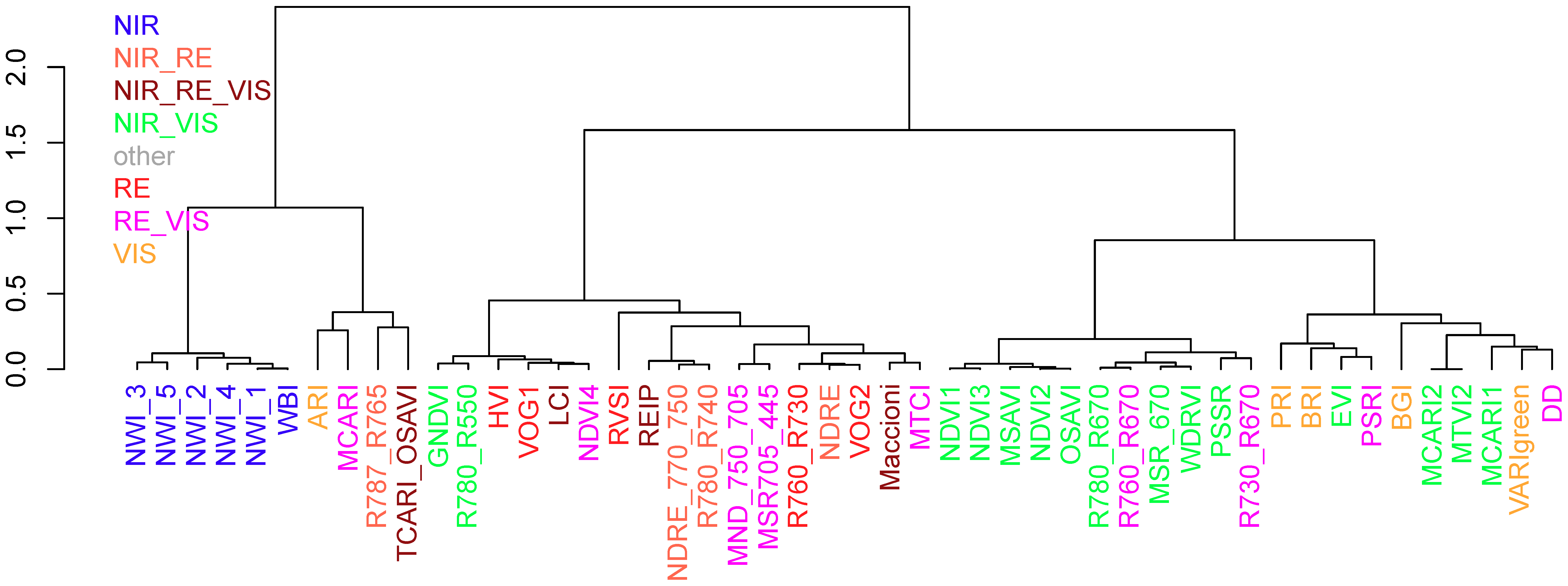
A cluster analysis was conducted based on the coefficients of determination for all trait*index*date combinations for comparing the initial index grouping according to the spectral regions with the grouping on the basis of the effective performance for all considered plant traits. For the full data, the clustering grouped the indices into two first-order branches. The NIR-based water band indices formed the most homogeneous group with a uniform second-order branch in the full data (Figure 10). The VIS indices were grouped in the second branch within the same first-order branch as the NIR indices, together with TCARI_OSAVI, R787_765, MCARI, DD, and PSRI as well as the NIR/VIS indices EVI, MCARI1, MCARI2, and MTVI2. The second first-order branch was subdivided into two branches as well: One dominated by most NIR/VIS indices, in addition to the R730_R670 and R760_R670, and the other branch containing most red edge-based indices as well as the NIR/green indices GNDVI and R780_R550. The grouping into four main groups was similar in all four datasets (not shown). In addition to the consistent groupings of the water-band indices, some indices were consistently grouped closely together: PRI + BRI, MCARI2 + MTVI2, TCARI_OSAVI + R787_R765, NDRE_770_750 + REIP + R780_R740, GNDVI + R780_R550, MND_750_705 + MSR705_445, R760_R730 + NDRE + VOG2 as well as HVI + VOG1+ LCI + NDVI4.
4. Discussion
This study evaluated the influence of the selection of measurement stages/dates and spectral vegetation indices (SVIs) on the estimation of various GNup-related N traits.
4.1. In-Season Estimation of Grain N Uptake and Contributing N Traits
Similar to grain yield (GY), GNup is formed over time but relies substantially more on the pre-anthesis component—Nup until anthesis—and its efficient translocation (NTEff). The resulting N translocation (NT) contributed on average ≈96% to GNup in RF and ≈91% in Cont and SD1, respectively, in the present data [12]. Although GNup was reduced by ≈9% in RF and increased by 5% in SD1, compared with Cont, NTEff (−8%), and NT (−5%, not significant) which were affected only in RF. The N harvest index (NHI) varied little between cultivars but was substantially higher than the DM harvest index (NHI ≈0.78 in RF, 0.84 in Cont and 0.85 in SD1). However, total Nup differed substantially both in the ‘agronomic’ datasets and between cultivars within the MP*N combinations. The fact that GNup was not closely related to GNC (R2 = 0.38 ***) in the full data [12] explains that the seasonal R2 patterns and the index rankings of GNup and GNC differed substantially. However, considering the high contribution of NT to GNup [12], high R2 values were reached for GNup already at stem elongation, the phase of maximum Nup [70]. The ear emergence stage was not suitable for detecting GNup and total Nup, which is likely an effect of phenological shifts that impact the spectral signal [71]. Although the seasonal pattern is consistent with previous years in the same environment [26], other studies recommend ear emergence for wheat [28] or anthesis for spring barley [72], indicating that the variation in ear emergence should be accounted for, depending on the underlying treatments.
Both the similar temporal R2 patterns and index rankings for total Nup as for GNup are in accordance with the close relationship between both traits (R2 = 0.88 *** in the full data and R2 = 0.64–0.97 within the MP*N datasets; [12]), whereas NHI was poorly (R2 = 0.17 * in the full data) or not (in MP*N) related to GNup. The estimation of NHI—only driven by its lower values in RF compared with Cont and SD1—may relate to the detection of differences in leaf senescence. Testing the spectral estimation of various biomass and N traits for phenotyping breeding lines, Frels et al. found useful relationships for NHI only in one of two years from the TCARI_OSAVI. In contrast to the present study, they also reported moderate, yet year-dependent, correlations for PANup; however, for a substantially broader data range in both traits.
The clear advantage of most red edge (RE)-based indices for most Nup traits is well in line with previous findings regarding the higher sensitivity of the RE reflection for overcoming saturation in the red region and for estimating the N status [27,54,73,74,75]. Thus, in particular NIR/RE indices that replaced the VIS band with a RE band [76] performed well. In contrast, the placement of the right-sided band appeared to be less crucial as indicated by the similarity in rankings from the R760_R730, R780_R740, NDRE, and NDRE_770_750 as well as of the LCI and the Maccioni index. Thus, the Maccioni index was previously recommended for GNup and NupEff [28], the NDRE_770_750 [26] and the REIP [77] for GNup, and the R780_740 for total Nup and for N use efficiency [27]. In contrast, some RE/VIS indices—notably the NDVI4, MTCI, MSR_705_445 and MND_750_705—ranked similarly to each other, but rarely best for any of the traits.
The comparable seasonal R2 pattern and index rankings for GNup as for total Nup at anthesis relates to the correlations between the traits (r = 0.48 ***; not shown). However, GNup was better assessed than vegetative Nup, possibly owing to the stage-specific sampling at anthesis, including a sampling interval of a few days, which reduced the variance in vegetative Nup. The mostly better detection of Nup of leaves than that of stems and spikes/chaff confirms results on spring barley [18] and is plausible, considering that the sensor predominantly detects the horizontally aligned leaf blades [78]. Thus, the observed detection of other organs may indicate rather indirect relationships via correlations with leaf traits. In contrast to anthesis Nup, vegetative Nup at maturity was substantially influenced by the reduced NTEff as introduced by reduced fungicide, which correlated with total leaf Nup at maturity (full data: r = 0.79 ***; not shown). Thus, indices suited for NTEff as well as for NC (R787_R765 and TCARI_OSAVI) were able to detect vegetative Nup at maturity in the agronomic data (Figure 7), but not the cultivar differences in MP*N. The similarly high rankings of both indices for many organ-level NC and Nup traits at maturity, NTEff, and NHI suggest a specific senescence sensitivity of these indices, because all these traits were altered by fungicide and N level effects [12]. This is in line with previous recommendations of these indices for retrieving NC in grassland [52] or chlorophyll [55], respectively.
4.2. Estimation of N Concentration Traits
The estimation of NC or chlorophyll content previously focused on leaf NC or NC of the total plant for optimizing N fertilization before anthesis [15]. However, the resulting N status at anthesis and grain filling is crucial for the formation of GY and GNup as well. Although RE/VIS indices previously optimized for leaf NC or chlorophyll content including the DD [60], MND_750_705, MSR_705_445 [62], and MTCI [63], ranked high for either one of the leaf layers, the VIS indices blue/red pigment index (BRI) and BGI were more consistent over time, for all three leaf layers and both in the agronomic and the MP*N approaches. Blue bands were less commonly used, but the BGI was also confirmed for chlorophyll retrieval in barley [79] and vine [48], in contrast to the BRI which was found less useful [48]. Such VIS indices are interesting because they are also available from simple red-green-blue (RGB) cameras [80]. Similar to Nup, NC of vegetative organs at maturity relates to variation in NTEff. Thus, the fungicide-related variation in the full data was captured by indices sensitive to senescence, whereas in the MP*N data, cultivars may not have sufficiently differed in NTEff.
4.3. Stability of Index Rankings by Datasets and Index Grouping
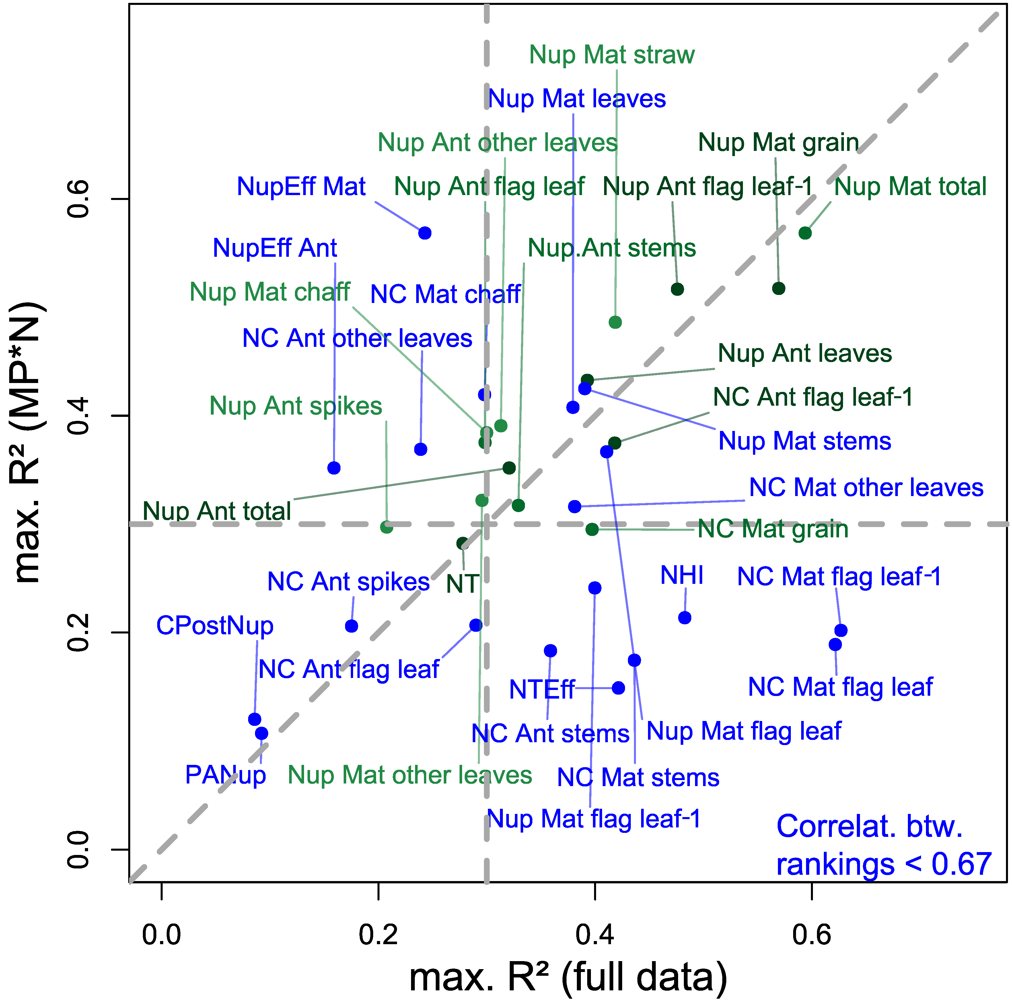
Year and treatment effects can be substantial, particularly on the derived N traits [20]; therefore, the comparison of index rankings addresses the influence of the underlying treatments. Similarly as for most Nup traits, the constant index rankings found for the important traits GNup and GNC are promising (Table 4; Figure 11). In contrast, trait variation introduced by N fertilization and differing fungicide intensities in the agronomic data may explain substantially differing index rankings (correlations between rankings < 0.67; blue colored in Figure 11) for many maturity-related NC and Nup traits. Mostly, those traits were not reliably assessed in MP*N but they were in the full data approach (bottom right quadrant in Figure 11). While indices selected for green-colored traits (transferable rankings) are promising for a more independent application, the index selection for blue-colored traits would require more consideration of the underlying treatments and/or trial environments.
The SVI clustering confirms the similarity in the index rankings and indicates that most SVIs grouped together by spectral bands gather similar canopy information. This is particularly the case for the NIR-based indices, which include the same water absorption band, as well as for the VIS indices, whereas the delimitation of RE-SVIs was less stringent. The similar grouping of the R787_R765 and the TCARI_OSAVI with VIS indices is in line with their discussed sensitivity of senescence-related pigment information. Similarly, RE/VIS indices, which were previously optimized for pigment detection (DD, MCARI, and PSRI [43,61,62]), were grouped together with VIS indices. Some RE/VIS indices based on the R670 band being grouped with the NIR/VIS indices support that choosing an upper band left to the NIR plateau had little impact compared to NIR/VIS indices similar to the NDVI.
The hyperspectral data used in this study yields optimized narrow-band SVIs. The information of relevant spectral bands used by these SVIs can be transferred to the band selection and the design of optimum multispectral sensors. Such sensors are less expensive, more robust and therefore better suited to be used by practitioners on tractors or drone platforms. Further aspects of view geometry, sensor resolution, and illumination conditions need to be addressed in this context.
5. Conclusions
Aiming at exploiting spectral proximal sensing for practical use in agronomic field trials, optimizations are required in the selection of (i) vegetation indices depending on the sensor and (ii) suitable growth stages for measurements, while a better understanding of the traits contributing to final GNup and their treatment response is equally important [12] for understanding (iii) the trait detection. With respect to (i), the results confirm the usefulness of NIR/red edge indices. For (ii), although the milk ripeness stage was generally best suited, moderate relationships observed already at stem elongation have the advantage of seasonally earlier estimations. In contrast, the ear emergence/anthesis phase should be avoided, probably owing to phenological shifts among cultivars. With respect to (iii), the results suggest that GNup is well estimated spectrally, similarly to total Nup under various trial conditions, whereas partitioning to the grain is not generally visible to the sensor. Although leaf information was better detected, N status of other organs could be moderately estimated as well, however the mechanism of the organ-specific detection may be indirect and should be further evaluated. The N translocation could be estimated in a similar manner as the closely related Nup at anthesis. Several traits—including most vegetative NC and Nup traits at maturity, NHI, and NTEff—were detected in the context of accelerated senescence without leaf fungicide in RF, but not for genotypic variation in MP*N.
Supplementary Materials
The following are available online at https://www.mdpi.com/1424-8220/19/21/4640/s1. Table S1: List of plant traits considered in this study, grouped by trait groups. Figure S1: Field trial measurements on 21 June 2017, colored by the values of the simple ratio index R760/R730. Figure S2: Plot-level spectra acquired on 31 March (leaf development, left), 17 May (stem elongation; middle) and 4 July 2017 (soft dough; right). Figure S3: The influence of the measurement date (year/month/day) on the trait estimation (Cont_SD1/Cont_RF/averaged form the six MP*N datasets). Figure S4: The index suitability by target trait. Figure S5: Seasonal coefficients of determination (R2) reached from all indices for grain N uptake (GNup), total Nup at maturity, and the N harvest index (NHI) for the Cont_SD1 and the Cont_RF data. Figure S6: Consistency between WMMRS-index rankings from the MP*N datasets (y-axis; Figure Figure 9b) and the agronomic datasets (x-axis; Figure Figure 9a) for all considered plant traits.
Author Contributions
L.P. and U.S. conceived and designed the experiment and wrote the manuscript; L.P. conducted the experiment and analyzed the data.
Funding
This research was funded by the DFG (German Research Foundation)-funded project SCHM 1456/6-1 and was also in part supported by funds of the Federal Ministry of Food and Agriculture (BMEL) in the project ‘Green Windows’ (28-1-B3.030-16).
Acknowledgments
The authors are grateful to Claudia Buchhart and Moritz Germer for support with the analysis of reference traits and to Jürgen Plass for support with spectral measurements. The authors gratefully acknowledge helpful suggestions on the manuscript by three anonymous reviewers.
Conflicts of Interest
The authors declare no conflicts of interest.
References
- Dawson, J.C.; Huggins, D.R.; Jones, S.S. Characterizing nitrogen use efficiency in natural and agricultural ecosystems to improve the performance of cereal crops in low-input and organic agricultural systems. Field Crops Res. 2008, 107, 89–101. [Google Scholar] [CrossRef]
- Hawkesford, M.J. Reducing the reliance on nitrogen fertilizer for wheat production. J. Cereal Sci. 2014, 59, 276–283. [Google Scholar] [CrossRef] [PubMed]
- Olesen, J.E.; Jørgensen, L.N.; Mortensen, J.V. Irrigation strategy, nitrogen application and fungicide control in winter wheat on a sandy soil. II. Radiation interception and conversion. J. Agric. Sci. 2000, 134, 13–23. [Google Scholar] [CrossRef]
- Varga, B.; Svečnjak, Z.; Maćešić, D.; Uher, D. Winter wheat cultivar responses to fungicide application are affected by nitrogen fertilization rate. J. Agron. Crop Sci. 2005, 191, 130–137. [Google Scholar] [CrossRef]
- Ishikawa, S.; Hare, M.C.; Kettlewell, P.S. Effects of strobilurin fungicide programmes and fertilizer nitrogen rates on winter wheat: Leaf area, dry matter yield and nitrogen yield. J. Agric. Sci. 2012, 150, 427–441. [Google Scholar] [CrossRef]
- Mourtzinis, S.; Marburger, D.; Gaska, J.; Diallo, T.; Lauer, J.G.; Conley, S. Corn, soybean, and wheat yield response to crop rotation, nitrogen rates, and foliar fungicide application. Crop Sci. 2017, 57, 983–992. [Google Scholar] [CrossRef]
- Ding, D.; Feng, H.; He, J.Q.; Zou, F.; Jin, J.M. Modifying winter wheat sowing date as an adaptation to climate change on the Loess Plateau. Agron. J. 2016, 53–63. [Google Scholar] [CrossRef]
- Yin, L.; Dai, X.; He, M. Delayed sowing improves nitrogen utilization efficiency in winter wheat without impacting yield. Field Crops Res. 2018, 221, 90–97. [Google Scholar] [CrossRef]
- Rasmussen, I.S.; Thorup-Kristensen, K. Does earlier sowing of winter wheat improve root growth and N uptake? Field Crops Res. 2016, 196, 10–21. [Google Scholar] [CrossRef]
- Milford, G.F.J.; Penny, A.; Prew, R.D.; Darby, R.J.; Todd, A.D. Effects of previous crop, sowing date, and winter and spring applications of nitrogen on the growth, nitrogen uptake and yield of winter wheat. J. Agric. Sci. 1993, 121, 1–12. [Google Scholar] [CrossRef]
- Ferrise, R.; Triossi, A.; Stratonovitch, P.; Bindi, M.; Martre, P. Sowing date and nitrogen fertilisation effects on dry matter and nitrogen dynamics for durum wheat: An experimental and simulation study. Field Crops Res. 2010, 117, 245–257. [Google Scholar] [CrossRef]
- Prey, L.; Germer, M.; Schmidhalter, U. Temporal and Organ-specific Responses in NUE Traits to N Fertilization, Fungicide Intensity and Early Sowing in Winter Wheat Cultivars. Agronomy 2019, 9, 313. [Google Scholar] [CrossRef]
- Nguyen, G.N.; Kant, S. Improving nitrogen use efficiency in plants: Effective phenotyping in conjunction with agronomic and genetic approaches. Funct. Plant Biol. 2018, 45, 606–619. [Google Scholar] [CrossRef]
- White, J.W.; Andrade-sanchez, P.; Gore, M.A.; Bronson, K.F.; Coffelt, T.A.; Conley, M.M.; Feldmann, K.A.; French, A.N.; Heun, J.T.; Hunsaker, D.J.; et al. Field Crops Research Field-based phenomics for plant genetics research. Field Crops Res. 2012, 133, 101–112. [Google Scholar] [CrossRef]
- Diacono, M.; Rubino, P.; Montemurro, F. Precision nitrogen management of wheat. A review. Agron. Sustain. Dev. 2013, 33, 219–241. [Google Scholar] [CrossRef]
- Bancal, M.O.; Roche, R.; Bancal, P. Late foliar diseases in wheat crops decrease nitrogen yield through N uptake rather than through variations in N remobilization. Ann. Bot. 2008, 102, 579–590. [Google Scholar] [CrossRef]
- Barraclough, P.B.; Lopez-Bellido, R.; Hawkesford, M.J. Genotypic variation in the uptake, partitioning and remobilisation of nitrogen during grain-filling in wheat. Field Crops Res. 2014, 156, 242–248. [Google Scholar] [CrossRef]
- Barmeier, G.; Schmidhalter, U. High-Throughput Field Phenotyping of Leaves, Leaf Sheaths, Culms and Ears of Spring Barley Cultivars at Anthesis and Dough Ripeness. Front. Plant Sci. 2017, 8, 1–16. [Google Scholar] [CrossRef]
- Erdle, K.; Mistele, B.; Schmidhalter, U. Spectral high-throughput assessments of phenotypic differences in biomass and nitrogen partitioning during grain filling of wheat under high yielding Western European conditions. Field Crops Res. 2013, 141, 16–26. [Google Scholar] [CrossRef]
- Prey, L.; Kipp, S.; Hu, Y.; Schmidhalter, U. Nitrogen Use Efficiency and Carbon Traits of High-Yielding European Hybrid vs. Line Winter Wheat Cultivars: Potentials and Limitations. Front. Plant Sci. 2019, 9, 1988. [Google Scholar] [CrossRef] [Green Version]
- Kong, L.; Xie, Y.; Hu, L.; Feng, B.; Li, S. Remobilization of vegetative nitrogen to developing grain in wheat (Triticum aestivum L.). Field Crops Res. 2016, 196, 134–144. [Google Scholar] [CrossRef]
- Raun, W.R.; Solie, J.B.; Johnson, G.V.; Stone, M.L.; Lukina, E.V.; Thomason, W.E.; Schepers, J.S. In-Season Prediction of Potential Grain Yield in Winter Wheat Using Canopy Reflectance. Agron. J. 2001, 93, 131. [Google Scholar] [CrossRef]
- Freeman, K.W.; Raun, W.R.; Johnson, G.V.; Mullen, R.W.; Stone, M.L.; Solie, J.B. Late-season prediction of wheat grain yield and grain protein. Commun. Soil Sci. Plant Anal. 2003, 34, 1837–1852. [Google Scholar] [CrossRef]
- Prasad, B.; Carver, B.F.; Stone, M.L.; Babar, M.A.; Raun, W.R.; Klatt, A.R. Genetic analysis of indirect selection for winter wheat grain yield using spectral reflectance indices. Crop Sci. 2007, 47, 1416–1425. [Google Scholar] [CrossRef]
- Prasad, B.; Carver, B.F.; Stone, M.L.; Babar, M.A.; Raun, W.R.; Klatt, A.R. Potential use of spectral reflectance indices as a selection tool for grain yield in winter wheat under great plains conditions. Crop Sci. 2007, 47, 1426–1440. [Google Scholar] [CrossRef]
- Prey, L.; Schmidhalter, U. Simulation of satellite reflectance data using high-frequency ground based hyperspectral canopy measurements for in-season estimation of grain yield and grain nitrogen status in winter wheat. ISPRS J. Photogramm. Remote Sens. 2019, 149, 176–187. [Google Scholar] [CrossRef]
- Pavuluri, K.; Chim, B.K.; Griffey, C.A.; Reiter, M.S.; Balota, M.; Thomason, W.E. Canopy spectral reflectance can predict grain nitrogen use efficiency in soft red winter wheat. Precis. Agric. 2015, 16, 405–424. [Google Scholar] [CrossRef]
- Frels, K.; Guttieri, M.; Joyce, B.; Leavitt, B.; Baenziger, P.S. Evaluating canopy spectral reflectance vegetation indices to estimate nitrogen use traits in hard winter wheat. Field Crops Res. 2018, 217, 82–92. [Google Scholar] [CrossRef]
- Mistele, B.; Gutser, R.; Schmidhalter, U. Validation of field-scaled spectral measurements of the nitrogen status in winter wheat. In Proceedings of the 7th International Conference on Precision Agriculture and Other Precision Resources Management, Minneapolis, MN, USA, 25–28 July 2004; pp. 1187–1195. [Google Scholar]
- Mistele, B.; Schmidhalter, U. Tractor-based quadrilateral spectral reflectance measurements to detect biomass and total aerial nitrogen in winter wheat. Agron. J. 2010, 102, 499–506. [Google Scholar] [CrossRef]
- Babar, M.A.; Van Ginkel, M.; Reynolds, M.P.; Prasad, B.; Klatt, A.R. Heritability, correlated response, and indirect selection involving spectral reflectance indices and grain yield in wheat. Aust. J. Agric. Res. 2007, 58, 432–442. [Google Scholar] [CrossRef]
- Babar, M.A.; van Ginkel, M.; Klatt, A.R.; Prasad, B.; Reynolds, M.P. The Potential of Using Spectral Reflectance Indices to Estimate Yield in Wheat Grown Under Reduced Irrigation. Euphytica 2006, 150, 155–172. [Google Scholar] [CrossRef]
- Peñuelas, J.; Filella, I.; Biel, C.; Serrano, L.; Savé, R.; Save, R. The reflectance at the 950–970 nm region as an indicator of plant water status. Int. J. Remote Sens. 1993, 14, 1887–1905. [Google Scholar] [CrossRef]
- Huete, A.; Didan, K.; Miura, T.; Rodriguez, E.P.; Gao, X.; Ferreira, L.G. Overview of the radiometric and biophysical performance of the MODIS vegetation indices. Remote Sens. Environ. 2002, 83, 195–213. [Google Scholar] [CrossRef]
- Gitelson, A.; Kaufman, Y.J.; Merzlyak, M.N. Use of a green channel in remote sensing of global vegetation from EOS-MODIS. Remote Sens. Environ. 1996, 58, 289–298. [Google Scholar] [CrossRef]
- Haboudane, D.; Miller, J.R.; Pattey, E.; Zarco-Tejada, P.J.; Strachan, I.B. Hyperspectral vegetation indices and novel algorithms for predicting green LAI of crop canopies: Modeling and validation in the context of precision agriculture. Remote Sens. Environ. 2004, 90, 337–352. [Google Scholar] [CrossRef]
- Broge, N.H.; Leblanc, E. Comparing prediction power and stability of broadband and hyperspectral vegetation indices for estimation of green leaf area index and canopy chlorophyll density. Remote Sens. Environ. 2001, 76, 156–172. [Google Scholar] [CrossRef]
- Chen, J.M. Evaluation of vegetation indices and a modified simple ratio for boreal applications. Can. J. Remote Sens. 1996, 22, 229–242. [Google Scholar] [CrossRef]
- Cristiano, P.M.; Posse, G.; Di Bella, C.M.; Jaimes, F.R. Uncertainties in fPAR estimation of grass canopies under different stress situations and differences in architecture. Int. J. Remote Sens. 2010, 31, 4095–4109. [Google Scholar] [CrossRef]
- Erdle, K.; Mistele, B.; Schmidhalter, U. Spectral assessments of phenotypic differences in spike development during grain filling affected by varying N supply in wheat. J. Plant Nutr. Soil Sci. 2013, 176, 952–963. [Google Scholar] [CrossRef]
- Zhao, C.; Zhou, Q.; Wang, J.; Huang, W. Spectral indices redefined in detecting nitrogen availability for wheat canopy. Commun. Soil Sci. Plant Anal. 2004, 35, 853–864. [Google Scholar] [CrossRef]
- Li, F.; Miao, Y.; Hennig, S.D.; Gnyp, M.L.; Chen, X.; Jia, L.; Bareth, G. Evaluating hyperspectral vegetation indices for estimating nitrogen concentration of winter wheat at different growth stages. Precis. Agric. 2010, 11, 335–357. [Google Scholar] [CrossRef]
- Ustin, S.L.; Gitelson, A.A.; Jacquemoud, S.; Schaepman, M.; Asner, G.P.; Gamon, J.A.; Zarco-tejada, P. Remote Sensing of Environment Retrieval of foliar information about plant pigment systems from high resolution spectroscopy. Remote Sens. Environ. 2009, 113, S67–S77. [Google Scholar] [CrossRef]
- Takebe, M.; Yoneyama, T.; Inada, K.; Murakami, T. Spectral reflectance ratio of rice canopy for estimating crop nitrogen status. Plant Soil 1990, 122, 295–297. [Google Scholar] [CrossRef]
- Pearson, R.L.; Miller, L.D. Remote mapping of standing crop biomass for estimation of the productivity of the shortgrass prairie. In Remote Sensing of Environment, 8th ed.; Elsevier: Amsterdam, The Netherlands, 1972; p. 1355. [Google Scholar]
- Gitelson, A.A. Wide dynamic range vegetation index for remote quantification of biophysical characteristics of vegetation. J. Plant Physiol. 2004, 161, 165–173. [Google Scholar] [CrossRef]
- Gitelson, A.A.; Merzlyak, M.N.; Chivkunova, O.B. Optical properties and nondestructive estimation of anthocyanin content in plant leaves. Photochem. Photobiol. 2001, 74, 38–45. [Google Scholar] [CrossRef]
- Zarco-Tejada, P.J.; Berjón, A.; López-Lozano, R.; Miller, J.R.; Martín, P.; Cachorro, V.; González, M.R.; De Frutos, A. Assessing vineyard condition with hyperspectral indices: Leaf and canopy reflectance simulation in a row-structured discontinuous canopy. Remote Sens. Environ. 2005, 99, 271–287. [Google Scholar] [CrossRef]
- Peñuelas, J.; Filella, I.; Gamon, J.A. Assessment of photosynthetic radiation-use efficiency with spectral reflectance. New Phytol. 1995, 131, 291–296. [Google Scholar] [CrossRef]
- Gitelson, A.A.; Kaufman, Y.J.; Stark, R.; Rundquist, D. Novel algorithms for remote estimation of vegetation fraction. Remote Sens. Environ. 2002, 80, 76–87. [Google Scholar] [CrossRef] [Green Version]
- Barnes, E.M.; Clarke, T.R.; Richards, S.E.; Colaizzi, P.D.; Haberland, J.; Kostrzewski, M.; Waller, P.; Choi, C.; Riley, E.; Thompson, T.; et al. Coincident detection of crop water stress, nitrogen status and canopy density using ground based multispectral data. In Proceedings of the Fifth International Conference on Precision Agriculture, Bloomington, MN, USA, 16–19 July 2000; Volume 1619, pp. 16–19. [Google Scholar]
- Fava, F.; Colombo, R.; Bocchi, S.; Meroni, M.; Sitzia, M.; Fois, N.; Zucca, C. Identification of hyperspectral vegetation indices for Mediterranean pasture characterization. Int. J. Appl. Earth Obs. Geoinf. 2009, 11, 233–243. [Google Scholar] [CrossRef]
- Maccioni, A.; Agati, G.; Mazzinghi, P. New vegetation indices for remote measurement of chlorophylls based on leaf directional reflectance spectra. J. Photochem. Photobiol. 2001, 61, 52–61. [Google Scholar] [CrossRef]
- Guyot, G.; Baret, F.; Major, D.J. High spectral resolution: Determination of spectral shifts between the red and infrared. Int. Arch. Photogramm. Remote Sens. 1988, 11, 750–760. [Google Scholar]
- Haboudane, D.; Miller, J.R.; Tremblay, N.; Zarco-Tejada, P.J.; Dextraze, L. Integrated narrow-band vegetation indices for prediction of crop chlorophyll content for application to precision agriculture. Remote Sens. Environ. 2002, 81, 416–426. [Google Scholar] [CrossRef]
- Gitelson, A.; Merzlyak, M.; Lichtenthaler, H. Detection of red edge position and chlorophyll content by reflectance measurements near 700 nm. J. Plant Physiol. 1996, 148, 501–508. [Google Scholar] [CrossRef]
- Jasper, J.; Reusch, S.; Link, A. Active sensing of the N status of wheat using optimized wavelength combination: Impact of seed rate, variety and growth stage. Precis. Agric. 2009, 9, 23–30. [Google Scholar]
- Merton, R. Monitoring community hysteresis using spectral shift analysis and the red-edge vegetation stress index. In Proceedings of the Seventh Annual JPL Airborne Earth Science Workshop; JPL: Pasadena, CA, USA, 1998; pp. 12–16. [Google Scholar]
- Vogelmann, J.E.; Rock, B.N.; Moss, D.M. Red edge spectral measurements from sugar maple leaves. Remote Sens. 1993, 14, 1563–1575. [Google Scholar] [CrossRef]
- Maire, G.; Franc, C.; Dufre, E. Towards universal broad leaf chlorophyll indices using PROSPECT simulated database and hyperspectral reflectance measurements. Remote Sens. Environ. 2004, 89, 1–28. [Google Scholar] [CrossRef]
- Daughtry, C.S.T.; Walthall, C.L.; Kim, M.S.; de Colstoun, E.B.; McMurtrey, J. Estimating corn leaf chlorophyll concentration from leaf and canopy reflectance. Remote Sens. Environ. 2000, 74, 229–239. [Google Scholar] [CrossRef]
- Sims, D.A.; Gamon, J.A. Relationships between leaf pigment content and spectral reflectance across a wide range of species, leaf structures and developmental stages. Remote Sens. Environ. 2002, 81, 337–354. [Google Scholar] [CrossRef]
- Dash, J.; Curran, P.J. The MERIS terrestrial chlorophyll index. In Proceedings of the MERIS User Workshop, Frascati, Italy, 10–13 November 2003; Volume 11. [Google Scholar]
- Gitelson, A.; Merzlyak, M.N. Quantitative estimation of chlorophyll-a using reflectance spectra: Experiments with autumn chestnut and maple leaves. J. Photochem. 1994, 22, 247–252. [Google Scholar] [CrossRef]
- Erdle, K.; Mistele, B.; Schmidhalter, U. Comparison of active and passive spectral sensors in discriminating biomass parameters and nitrogen status in wheat cultivars. Field Crops Res. 2011, 124, 74–84. [Google Scholar] [CrossRef]
- Gutierrez, M.; Reynolds, M.P.; Klatt, A.R. Effect of leaf and spike morphological traits on the relationship between spectral reflectance indices and yield in wheat. Int. J. Remote Sens. 2015, 36, 701–718. [Google Scholar] [CrossRef]
- Gutierrez, M.; Reynolds, M.P.; Raun, W.R.; Stone, M.L.; Klatt, A.R. Spectral water indices for assessing yield in elite bread wheat genotypes under well-irrigated, water-stressed, and high-temperature conditions. Crop Sci. 2010, 50, 197–214. [Google Scholar] [CrossRef]
- Gutierrez, M.; Reynolds, M.; Klatt, A. Association of water spectral indices with plant and soil water relations in contrasting wheat genotypes. J. Exp. Bot. 2010, 61, 3291–3303. [Google Scholar] [CrossRef] [PubMed] [Green Version]
- Becker, E.; Schmidhalter, U. Evaluation of Yield and Drought Using Active and Passive Spectral Sensing Systems at the Reproductive Stage in Wheat. Front. Plant Sci. 2017, 8. [Google Scholar] [CrossRef] [PubMed] [Green Version]
- Spratt, E.D.; Gasser, J.K.R. Effects of fertilizer-nitrogen and water supply on distribution of dry matter and nitrogen between the different parts of wheat. Can. J. Plant Sci. 1970, 50, 613–625. [Google Scholar] [CrossRef]
- Pimstein, A.; Eitel, J.U.H.; Long, D.S.; Mufradi, I.; Karnieli, A.; Bonfil, D.J. A spectral index to monitor the head-emergence of wheat in semi-arid conditions. Field Crops Res. 2009, 111, 218–225. [Google Scholar] [CrossRef] [Green Version]
- Barmeier, G.; Hofer, K.; Schmidhalter, U. Mid-season prediction of grain yield and protein content of spring barley cultivars using high-throughput spectral sensing. Eur. J. Agron. 2017, 90, 108–116. [Google Scholar] [CrossRef]
- Boochs, F.; Kupfer, G.; Dockter, K.; Kühbauch, W. Shape of the red edge as vitality indicator for plants. Int. J. Remote Sens. 1990, 11, 1741–1753. [Google Scholar] [CrossRef]
- Guo, B.B.; Qi, S.L.; Heng, Y.R.; Duan, J.Z.; Zhang, H.Y.; Wu, Y.P.; Feng, W.; Xie, Y.X.; Zhu, Y.J. Remotely assessing leaf N uptake in winter wheat based on canopy hyperspectral red-edge absorption. Eur. J. Agron. 2017, 82, 113–124. [Google Scholar] [CrossRef]
- Prey, L.; Schmidhalter, U. Sensitivity of Vegetation Indices for Estimating Vegetative N Status in Winter Wheat. Sensors 2019, 19, 3712. [Google Scholar] [CrossRef]
- Datt, B. A new reflectance index for remote sensing of chlorophyll content in higher plants: Tests using Eucalyptus leaves. J. Plant Physiol. 1999, 154, 30–36. [Google Scholar] [CrossRef]
- Prey, L.; Hu, Y.; Schmidhalter, U. Spectral sensing traits of nitrogen use efficiency in hybrid and line wheat cultivars. In Tagungsband der 68. Jahrestagung der Vereinigung der Pflanzenzüchter und Saatgutkaufleute Österreichs, 20–22 November 2017; Brandstetter, A., Geppner, M., Eds.; Universität für Bodenkultur Wien: Vienna, Austria, 2018; pp. 59–62. [Google Scholar]
- Huang, W.; Niu, Z.; Wang, J.; Liu, L.; Zhao, C.; Liu, Q. Identifying crop leaf angle distribution based on two-temporal and bidirectional canopy reflectance. IEEE Trans. Geosci. Remote Sens. 2006, 44, 3601–3608. [Google Scholar] [CrossRef]
- Aasen, H.; Burkart, A.; Bolten, A.; Bareth, G. ISPRS Journal of Photogrammetry and Remote Sensing Generating 3D hyperspectral information with lightweight UAV snapshot cameras for vegetation monitoring: From camera calibration to quality assurance. ISPRS J. Photogramm. Remote Sens. 2015, 108, 245–259. [Google Scholar] [CrossRef]
- Baresel, J.P.; Rischbeck, P.; Hu, Y.; Kipp, S.; Hu, Y.; Barmeier, G.; Mistele, B. Use of a digital camera as alternative method for non-destructive detection of the leaf chlorophyll content and the nitrogen nutrition status in wheat. Comput. Electron. Agric. 2017, 140, 25–33. [Google Scholar] [CrossRef]
Figure 1.
(a) Seasonal index development of the NDRE_770_750 colored by the main plot (Cont: Control; RF: reduced fungicide; SD1: sowing date 1) and N fertilization treatments (N1; N2). The last measurement date was not included in the analysis due to advanced senescence. Gray labels indicate growth stages; colored background bars indicate the reference plant sampling at anthesis and maturity. Days after sowing refer to the Cont and RF plots. (b) Plot-level spectra acquired on 21 June 2017 with band position of the tested spectral vegetation indices, colored by index groups: near-infrared (NIR: >765 nm), visible (VIS: <700 nm), and the extended red edge (RE: 700–765 nm). The spectra are colored by the values of grain nitrogen uptake (yellow: low, blue: high). The dashed line represents the coefficient of variation of the reflectance. Refer to Figure S2 for spectra of selected dates.

Figure 2.
Datasets used for evaluating trait–index relationships. Three ‘agronomic’ datasets correspond to data of the whole trial (‘full data’), the combined main plots (MP) control (Cont) and reduced fungicide (RF; Cont_RF), as well as the combined MPs Cont and sowing date 1 (SD1; Cont_SD1). MP*N represents the testing within the six subplots as the interaction of main plots (MP) and N fertilization level (N; N1: 60 kg N ha−1; N2: 60 kg N ha−1). In SD1, five plots were removed due to missing data or plot damage.

Figure 3.
The influence of the measurement date (year/month/day) on the trait estimation in the full data: Maximum coefficients of determination (R2) found from the 48 tested spectral vegetation indices (SVIs). See Figure S3 for results of Cont_SD1, Cont_RF, and MP*N datasets.
Figure 3.
The influence of the measurement date (year/month/day) on the trait estimation in the full data: Maximum coefficients of determination (R2) found from the 48 tested spectral vegetation indices (SVIs). See Figure S3 for results of Cont_SD1, Cont_RF, and MP*N datasets.

Figure 4.
The index suitability by target trait: (a) full data; (b) average from the six MP*N datasets. Maximum coefficients of determination (R2) found for each index*trait combination from 10 measurement dates. Gray lines delimit index and trait groups. See Figure S4 for results of Cont_SD1 and Cont_RF.

Figure 5.
Seasonal coefficients of determination (R2) reached from all indices for (a) grain N uptake (GNup); (b) total Nup at maturity; and (c) the N harvest index (NHI) in the full data and the main plot*N (MP*N) approach. Lines are colored according to the spectral regions included in the index equations (Figure 1b). The results for the MP*N combinations are averaged from the results within the six MP*N combinations. Horizontal gray lines indicate significance thresholds on different levels. Thick lines and index labels indicate results of the best indices based on the WMMRS-ranking of the ‘agronomic’ approach. Refer to Figure S5 for results of the Cont_SD1 and Cont_RF datasets. d.a.s.: days after sowing.

Figure 6.
Relationships of (a) GNup, (b) total Nup and (c) N harvest index on most suited dates (year/month/day; selected based on Table 3) with rank-based best indices. Colored thin lines correspond to linear regressions for the MP*N subsets, dashed blue and red lines correspond to Cont_SD1 and Cont_RF, respectively, and the dashed gray lines indicate the full dataset. R2 values are colored accordingly.

Figure 7.
Seasonal coefficients of determination (R2) reached from all indices for selected N traits in (a) ther full data and in (b) the main plot*N (MP*N) data, as well as the trait–index relationships from the WMMRS-based best index/date (year/month/day) combinations. Lines are colored according to the spectral regions included in the index equations (Figure 1b). The results for MP*N are averaged from the results within the six MP*N combinations. Horizontal gray lines indicate significance thresholds on different levels. Thick lines and index labels indicate results of the best indices based on the WMMRS-ranking of the ‘agronomic’ approach. For the scatterplots, colored thin lines correspond to linear regressions for the MP*N subsets, dashed blue and red lines correspond to Cont_SD1 and Cont_RF, respectively, and the dashed gray lines indicate the full datasets. R2 values are colored accordingly. d.a.s.: days after sowing.

Figure 8.
Seasonal coefficients of determination (R2) reached from all indices for selected N concentration (NC) traits in (a) the full data and in (b) the main plot*N (MP*N) data as well as the trait–index relationships from the best index/date (year/month/day) combination. Lines are colored according to the spectral regions included in the index equations (Figure 1b). The results for MP*N are averaged from the results within the six MP*N combinations. Horizontal gray lines indicate significance thresholds on different levels. Thick lines and index labels indicate results of the best indices based on the WMMRS-ranking of the ‘agronomic’ approach. For the scatterplots, colored thin lines correspond to linear regressions for the MP*N subsets, dashed blue and red lines correspond to Cont_SD1 and Cont_RF, respectively, and the dashed gray lines indicate the full datasets. R2 values are colored accordingly. d.a.s.: days after sowing.

Figure 9.
Weighted mean/maximum rank sums (WMMRS) for all evaluated trait*index combinations. (a) The combined WMMRS rankings from the three agronomic datasets (‘full data’, Cont_SD1, and Cont_RF). (b) WMMRS rankings from the six MP*N subsets, which were multiplied by three for direct comparison on the same numeric level. Rankings based on mean R2 across dates were double-weighted. For each trait, the value of nine corresponds to the average ranking across all indices. Blue cells indicate WMMRS values >15. Blue lines delimit index and trait groups, respectively. Rankings for trait*index combinations that did not exceed the threshold of maximum R2 values of 0.20 are not shown (white cells), being considered irrelevant.

Figure 10.
Cluster analysis based on Ward’s method on index kinship based on the performance for all dates and traits in the full data (n = 10*34 -> 340). Colors indicate initial index groups based on the included spectral regions (Figure 1b).
Figure 10.
Cluster analysis based on Ward’s method on index kinship based on the performance for all dates and traits in the full data (n = 10*34 -> 340). Colors indicate initial index groups based on the included spectral regions (Figure 1b).

Figure 11.
Relationship of trait-specific maximum relationships (R2; Figure 4) in the full data and the MP*N approach. The data is colored by Spearman’s ρ (green: ρ > 0.67, blue: ρ < 0.67) on the correlations between the WMMRS rankings of the ‘agronomic’ and the MP*N approach (Table 4). Dashed lines mark the 1:1 line and arbitrary R2 thresholds (0.3) for categorizing the traits by R2 values in both approaches.


Table 1.
Dates of spectral measurements (month/day) with days after sowing (d.a.s) in control (Cont) and reduced fungicide (RF) plots and dominant growth stages.
Table 1.
Dates of spectral measurements (month/day) with days after sowing (d.a.s) in control (Cont) and reduced fungicide (RF) plots and dominant growth stages.
| Date (Month/Day) | d.a.s. | Growth Stage |
|---|---|---|
| 03/31 | 159 | leaf development |
| 04/13 | 172 | tillering |
| 05/17 | 206 | stem elongation |
| 05/25 | 214 | booting |
| 06/01 | 221 | ear emergence |
| 06/08 | 228 | anthesis |
| 06/21 | 241 | early milk |
| 06/26 | 246 | late milk |
| 07/01 | 251 | early dough |
| 07/04 | 255 | soft dough |
Table 2.
List of spectral vegetation indices considered in this study. ‘R’ denotes the reflection in indicated wavebands.
Table 2.
List of spectral vegetation indices considered in this study. ‘R’ denotes the reflection in indicated wavebands.
| Index | Full name | Spectral | Equation | Reference |
|---|---|---|---|---|
| NWI-1 | Normalized water index 1 | NIR | [31,32] | |
| NWI-2 | Normalized water index 2 | NIR | [31,32] | |
| NWI-3* | Normalized water index 3 | NIR | [31] | |
| NWI-4* | Normalized water index 4 | NIR | [31] | |
| NWI-5 | Normalized water index 5 | NIR | [26] | |
| WBI | Water band index | NIR | [33] | |
| EVI | Enhanced vegetation index | NIR,VIS | [34] | |
| GNDVI | Green NDVI** | NIR,VIS | [35] | |
| MCARI1 | Modified chlorophyll absorption in reflectance index 1 | NIR,VIS | [36] | |
| MCARI2 | Modified chlorophyll absorption in reflectance index 2 | NIR,VIS | )/ (((2* | [36] |
| MSAVI | Modified soil-adjusted vegetation index | NIR,VIS | [37] | |
| MSR(MSR_670) | Modified simple ratio 670 | NIR,VIS | [38] | |
| MTVI2 | Modified triangular vegetation Index 2 | NIR,VIS | ) | [36] |
| NDVI1 | Normalized difference vegetation index 1 | NIR,VIS | [39] | |
| NDVI2 | Normalized difference vegetation index 2 | NIR,VIS | [19,40] | |
| NDVI3 | Normalized difference vegetation index 3 | NIR,VIS | [41] | |
| OSAVI | Optimized soil-adjusted vegetation index | NIR,VIS | [42] | |
| PSSR | Pigment specific simple ratio | NIR,VIS | [43] | |
| R780_R550 | NIR,VIS | [44] | ||
| R780_R670 | NIR,VIS | [45] | ||
| WDRVI | Wide dynamic range vegetation index | NIR,VIS | [46] | |
| ARI | Anthocyanin reflectance index | VIS | [47] | |
| BGI | Blue green pigment index | VIS | [48] | |
| BRI | Blue red pigment index | VIS | [48] | |
| PRI | Photochemical reflectance index | VIS | [49] | |
| VARIgreen | Visible atmospherically resistant vegetation index green | VIS | [50] | |
| NDRE | Normalized difference NIR/red edge index | NIR,RE | [51] | |
| R780_R740 | NIR,RE | [29] | ||
| NDRE_770_750 | NIR,RE | [26] | ||
| R787_R765 | NIR,RE | [52] | ||
| LCI | Leaf chlorophyll index | NIR,RE,VIS | *** | |
| Maccioni | Maccioni index | NIR,RE,VIS | [53] | |
| REIP | Red edge inflection point | NIR,RE,VIS | [54] | |
| TCARI_OSAVI | NIR,RE,VIS | 3*((-)-0.2*(-)*/)/ ( | [55] | |
| HVI | Hyperspectral vegetation index | RE | [56] | |
| R760_R730 | RE | [30,57] | ||
| RVSI | Red edge vegetation stress index | RE | [58] | |
| VOG1 | Vogelmann 1 | RE | [59] | |
| VOG2 | Vogelmann 2 | RE | [59] | |
| DD | Double difference index | RE,VIS | [60] | |
| MCARI | Modified chlorophyll absorption in reflectance index | RE,VIS | [61] | |
| MND_750_705 | Modified normalized difference 750/705 | RE,VIS | [62] | |
| MSR_705_445 | Modified simple ratio 705/445 | RE,VIS | [62] | |
| MTCI | MERIS**** terrestrial chlorophyll index | RE,VIS | [63] | |
| NDVI4 | Normalized difference vegetation index 4 | RE,VIS | [64] | |
| PSRI | Plant senescence reflectance index | RE,VIS | [62] | |
| R730_R670 | RE,VIS | [30] | ||
| R760_R670 | RE,VIS | [65] |
Table 3.
Best spectral vegetation indices (SVIs) based on the weighted mean/maximum-rank sums (WMMRS) from the ‘agronomic’ approach with its seasonally highest R2 value with significance (*** p < 0.001; ** p < 0.01; * p < 0.05; n.s.: not significant) and lowest root mean square error (RMSE) reached on the optimum date (month/day) in the different datasets: ‘Full data’, ‘Cont_SD1’, ‘Cont_RF’ as well as the six main plot*N level combinations (MP*N). Considering the six MP*N blocks as different environments, the results for MP*N are based on the average R2 and RMSE values from the six MP*N subsets. Due to slightly differing n (number of data points), the significance for MP*N was re-calculated based on the averaged thresholds in the six subsets. For nitrogen uptake (Nup), ‘Ant. Leaves’ and ‘Mat. Leaves’ refer to the aggregated values of all leaf layers. Abbreviations: NC: nitrogen content; Nup: nitrogen uptake; Ant.: anthesis; Mat.: maturity; PANup: post-anthesis N uptake; CPostNup: contribution of PANup to total Nup; NT: N translocation; NTEff: N matter translocation efficiency; NHI: N harvest index. Refer to Figure 5, Figure 7 and Figure 8 for seasonal R2-values of selected traits in the full data and MP*N.
| Seasonally Best R2 | Optimum Date (month/day) | RMSE | |||||||||||||||||
|---|---|---|---|---|---|---|---|---|---|---|---|---|---|---|---|---|---|---|---|
| Trait Group | Trait | Best SVI | WMMRS | Full Data | Cont_SD1 | Cont_RF | MP*N | Full Data | Cont_SD1 | Cont_RF | MP*N | Full Data | Cont_SD1 | Cont_RF | MP*N | ||||
| NC (%) | Ant. spikes | NDRE_770_750 | 13 | 0.16 | *** | 0.25 | *** | 0.09 | ** | 0.18 | * | 06/26 | 06/26 | 06/26 | 06/21 | 0.06 | 0.06 | 0.06 | 0.05 |
| Ant. stems | RVSI | 19 | 0.34 | *** | 0.44 | *** | 0.30 | *** | 0.12 | n.s. | 07/01 | 06/26 | 05/17 | 05/17 | 0.10 | 0.09 | 0.10 | 0.08 | |
| Ant. flag leaf | DD | 17 | 0.25 | *** | 0.20 | *** | 0.20 | *** | 0.16 | * | 05/25 | 05/25 | 05/25 | 05/25 | 0.19 | 0.20 | 0.20 | 0.18 | |
| Ant. flag leaf–1 | BGI | 19 | 0.30 | *** | 0.30 | *** | 0.27 | *** | 0.28 | ** | 06/08 | 06/08 | 06/08 | 06/08 | 0.20 | 0.20 | 0.20 | 0.17 | |
| Ant. other leaves | BGI | 36 | 0.24 | *** | 0.27 | *** | 0.25 | *** | 0.29 | ** | 06/08 | 06/08 | 07/01 | 06/08 | 0.24 | 0.23 | 0.24 | 0.21 | |
| Mat. grain | REIP | 17 | 0.38 | *** | 0.41 | *** | 0.41 | *** | 0.26 | ** | 05/25 | 06/26 | 05/25 | 05/25 | 0.14 | 0.14 | 0.13 | 0.09 | |
| Mat. chaff | TCARI_OSAVI | 18 | 0.30 | *** | 0.21 | *** | 0.28 | *** | 0.17 | * | 07/04 | 07/04 | 06/26 | 06/08 | 0.05 | 0.05 | 0.06 | 0.05 | |
| Mat. stems | TCARI_OSAVI | 17 | 0.44 | *** | 0.36 | *** | 0.38 | *** | 0.17 | * | 07/04 | 07/01 | 06/26 | 07/01 | 0.04 | 0.04 | 0.04 | 0.03 | |
| Mat. flag leaf | R787_R765 | 16 | 0.62 | *** | 0.08 | * | 0.69 | *** | 0.14 | * | 07/04 | 06/26 | 07/04 | 03/31 | 0.26 | 0.11 | 0.26 | 0.16 | |
| Mat. flag leaf–1 | MCARI | 17 | 0.49 | *** | 0.18 | *** | 0.59 | *** | 0.09 | n.s. | 07/04 | 07/01 | 07/04 | 07/01 | 0.16 | 0.08 | 0.16 | 0.09 | |
| Mat. other leaves | MCARI | 14 | 0.37 | *** | 0.15 | *** | 0.52 | *** | 0.13 | n.s. | 07/01 | 06/08 | 07/01 | 07/01 | 0.13 | 0.11 | 0.13 | 0.10 | |
| Direct Nup (kg N ha−1) | Ant. spikes | BRI | 13 | 0.21 | *** | 0.32 | *** | 0.19 | *** | 0.28 | ** | 06/26 | 07/01 | 06/26 | 06/26 | 5.2 | 4.5 | 5.4 | 4.8 |
| Ant. stems | NDRE_770_750 | 15 | 0.33 | *** | 0.36 | *** | 0.33 | *** | 0.28 | ** | 05/25 | 05/25 | 04/13 | 05/25 | 10.3 | 9.3 | 10.3 | 9.4 | |
| Ant. flag leaf | NDRE_770_750 | 13 | 0.30 | *** | 0.43 | *** | 0.22 | *** | 0.33 | *** | 07/04 | 07/04 | 07/04 | 07/04 | 5.6 | 4.8 | 6.2 | 4.9 | |
| Ant. flag leaf–1 | REIP | 14 | 0.40 | *** | 0.48 | *** | 0.43 | *** | 0.51 | *** | 05/25 | 06/21 | 06/08 | 06/08 | 3.8 | 3.5 | 3.5 | 3.1 | |
| Ant. other leaves | ARI | 14 | 0.16 | *** | 0.17 | *** | 0.30 | *** | 0.39 | *** | 06/26 | 05/17 | 04/13 | 04/13 | 4.4 | 4.3 | 3.8 | 3.3 | |
| Ant. leaves | NDRE_770_750 | 14 | 0.38 | *** | 0.47 | *** | 0.33 | *** | 0.43 | *** | 06/08 | 06/08 | 06/08 | 06/08 | 10.0 | 9.3 | 10.7 | 9.1 | |
| Mat. grain | NDRE_770_750 | 15 | 0.57 | *** | 0.53 | *** | 0.67 | *** | 0.52 | *** | 06/26 | 06/26 | 06/26 | 06/26 | 16.0 | 16.7 | 13.1 | 9.7 | |
| Mat. chaff | REIP | 14 | 0.25 | *** | 0.36 | *** | 0.24 | *** | 0.31 | *** | 06/26 | 06/26 | 04/13 | 06/26 | 1.5 | 1.3 | 1.5 | 1.3 | |
| Mat. stems | TCARI_OSAVI | 15 | 0.39 | *** | 0.27 | *** | 0.46 | *** | 0.18 | * | 06/26 | 07/01 | 06/26 | 07/01 | 3.1 | 2.7 | 3.0 | 2.6 | |
| Mat. flag leaf | TCARI_OSAVI | 19 | 0.39 | *** | 0.31 | *** | 0.43 | *** | 0.27 | ** | 07/04 | 07/04 | 07/04 | 07/01 | 2.2 | 0.8 | 2.4 | 1.2 | |
| Mat. flag leaf–1 | TCARI_OSAVI | 19 | 0.40 | *** | 0.22 | *** | 0.46 | *** | 0.14 | * | 07/04 | 07/01 | 07/04 | 07/01 | 0.8 | 0.5 | 0.8 | 0.5 | |
| Mat. other leaves | R787_R765 | 19 | 0.30 | *** | 0.50 | *** | 0.30 | *** | 0.32 | *** | 05/25 | 06/08 | 07/04 | 06/08 | 0.9 | 0.7 | 0.9 | 0.8 | |
| Mat. leaves | TCARI_OSAVI | 20 | 0.37 | *** | 0.22 | *** | 0.46 | *** | 0.23 | ** | 07/04 | 06/26 | 07/04 | 07/01 | 3.6 | 1.9 | 3.7 | 2.1 | |
| Ant. total | NDRE_770_750 | 14 | 0.32 | *** | 0.43 | *** | 0.27 | *** | 0.34 | *** | 05/25 | 06/08 | 06/08 | 06/08 | 23.4 | 20.6 | 24.4 | 21.3 | |
| Mat. total | NDRE_770_750 | 16 | 0.59 | *** | 0.57 | *** | 0.58 | *** | 0.57 | *** | 06/26 | 06/26 | 06/26 | 06/26 | 17.5 | 19.0 | 16.9 | 11.7 | |
| Mat. straw | TCARI_OSAVI | 18 | 0.42 | *** | 0.27 | *** | 0.51 | *** | 0.22 | ** | 06/26 | 06/26 | 06/26 | 04/13 | 6.9 | 5.2 | 6.6 | 5.0 | |
| Derived N | PANup (kg N ha−1) | RVSI | 17 | 0.09 | *** | 0.13 | *** | 0.11 | ** | 0.10 | n.s. | 06/26 | 05/17 | 06/26 | 07/04 | 23.9 | 22.4 | 24.1 | 19.6 |
| CPostNup | RVSI | 16 | 0.07 | ** | 0.11 | ** | 0.09 | ** | 0.10 | n.s. | 04/13 | 07/04 | 06/26 | 07/04 | 0.11 | 0.10 | 0.11 | 0.09 | |
| NT (kg N ha−1) | NDRE_770_750 | 13 | 0.28 | *** | 0.33 | *** | 0.26 | *** | 0.28 | ** | 06/08 | 06/08 | 06/08 | 06/08 | 21.1 | 19.2 | 21.7 | 19.7 | |
| NTEff | R787_R765 | 20 | 0.42 | *** | 0.07 | * | 0.54 | *** | 0.08 | n.s. | 07/04 | 05/17 | 07/04 | 03/31 | 0.03 | 0.02 | 0.03 | 0.02 | |
| NHI | NWI_2 | 15 | 0.32 | *** | 0.10 | ** | 0.46 | *** | 0.13 | n.s. | 07/04 | 06/08 | 07/04 | 06/01 | 0.03 | 0.02 | 0.03 | 0.02 | |
| NupEff Ant. | RVSI | 28 | 0.16 | *** | 0.23 | *** | 0.14 | *** | 0.33 | *** | 06/26 | 07/04 | 06/26 | 06/08 | 0.72 | 0.65 | 0.75 | 0.25 | |
| NupEff Mat. | R787_R765 | 32 | 0.24 | *** | 0.49 | *** | 0.16 | *** | 0.33 | *** | 06/26 | 06/26 | 06/26 | 05/25 | 0.59 | 0.47 | 0.62 | 0.18 | |
Table 4.
Spearman’s ρ and significance level (*** p < 0.001; ** p < 0.01; * p < 0.05; n.s.: not significant) of the correlations between the agronomic and the MP*N index rankings (Figure 9) by target trait. See Figure S6 for scatterplots between both rankings.
| NC | Nup | Derived N | ||||||
|---|---|---|---|---|---|---|---|---|
| Ant. spikes | −0.29 | * | Ant. spikes | 0.85 | *** | PANup | 0.06 | n.s. |
| Ant. stems | 0.02 | n.s. | Ant. stems | 0.89 | *** | CPostNup | −0.03 | n.s. |
| Ant. flag leaf | 0.30 | * | Ant. flag leaf | 0.90 | *** | NT | 0.97 | *** |
| Ant. flag leaf–1 | 0.92 | *** | Ant. flag leaf–1 | 0.92 | *** | NTEff | −0.22 | n.s. |
| Ant. other leaves | 0.45 | ** | Ant. other leaves | 0.84 | *** | NHI | −0.37 | * |
| Mat. grain | 0.91 | *** | Ant. leaves | 0.98 | *** | NupEff Ant. | 0.35 | * |
| Mat. chaff | 0.54 | *** | Mat. grain | 0.94 | *** | NupEff Mat. | 0.17 | n.s. |
| Mat. stems | −0.12 | n.s. | Mat. chaff | 0.78 | *** | |||
| Mat. flag leaf | −0.03 | n.s. | Mat. stems | 0.60 | *** | |||
| Mat. flag leaf–1 | 0.09 | n.s. | Mat. flag leaf | −0.34 | * | |||
| Mat. other leaves | 0.58 | *** | Mat. flag leaf–1 | −0.53 | *** | |||
| Mat. other leaves | 0.80 | *** | ||||||
| Mat. leaves | −0.33 | * | ||||||
| Ant. total | 0.95 | *** | ||||||
| Mat. total | 0.89 | *** | ||||||
| Mat. straw | 0.63 | *** | ||||||
© 2019 by the authors. Licensee MDPI, Basel, Switzerland. This article is an open access article distributed under the terms and conditions of the Creative Commons Attribution (CC BY) license (http://creativecommons.org/licenses/by/4.0/).
Share and Cite
MDPI and ACS Style
Prey, L.; Schmidhalter, U. Temporal and Spectral Optimization of Vegetation Indices for Estimating Grain Nitrogen Uptake and Late-Seasonal Nitrogen Traits in Wheat. Sensors 2019, 19, 4640. https://doi.org/10.3390/s19214640
AMA Style
Prey L, Schmidhalter U. Temporal and Spectral Optimization of Vegetation Indices for Estimating Grain Nitrogen Uptake and Late-Seasonal Nitrogen Traits in Wheat. Sensors. 2019; 19(21):4640. https://doi.org/10.3390/s19214640
Chicago/Turabian StylePrey, Lukas, and Urs Schmidhalter. 2019. "Temporal and Spectral Optimization of Vegetation Indices for Estimating Grain Nitrogen Uptake and Late-Seasonal Nitrogen Traits in Wheat" Sensors 19, no. 21: 4640. https://doi.org/10.3390/s19214640
Note that from the first issue of 2016, this journal uses article numbers instead of page numbers. See further details here.