A Note on Double Conformable Laplace Transform Method and Singular One Dimensional Conformable Pseudohyperbolic Equations

Abstract

The purpose of this article is to obtain the exact and approximate numerical solutions of linear and nonlinear singular conformable pseudohyperbolic equations and conformable coupled pseudohyperbolic equations through the conformable double Laplace decomposition method. Further, the numerical examples were provided in order to demonstrate the efficiency, high accuracy, and the simplicity of present method.

1. Introduction

In recent years, many mathematicians have been studying and discussing the linear and nonlinear fractional differential equations (FDEs) which arise in various fields of physical sciences, as well as in engineering. These types of equations play a significant role and also help to develop mathematical tools in order to understand fractional modelling.

However, there are many different methods to obtain exact and approximate solutions of these kinds of equations. In [1], the author point out a major flaw in the so-called conformable calculus. Recently, many researchers have also paid much attention to study the numerical and exact methods for finding the solution of conformable differential equations. In [2], the authors proposed so-called conformable derivatives. In [3], the conformable heat equation was studied. Similarly, in [4], the nonlinear conformable problems were also studied. The authors in [5] discussed the concepts underlying the formulation of operators capable of being interpreted as fractional derivatives or fractional integrals. In a very short period of time, many mathematicians became interested and provided mathematical models related to conformable derivatives, for the details we refer reader to see [6,7,8,9]. In [10,11], the conformable derivatives were applied to some problems in mechanics, and in [12] total frational derivative and directional fractional derivative of functions of several variables were studied.

In order to solve the conformable derivatives, the single Laplace transform method was first introduced and used in [13]. In [14], the idea was extended to the conformable double Laplace transform. In [15], the modified Laplace transform was applied to solve some ordinary differential equations in the frame work of a certain type generalized fractional derivatives. The authors in [16] applied the double Laplace decomposition method to solve singular linear and nonlinear one-dimensional pseudohyperbolic equations.

In this present research, the main objective is to solve linear and nonlinear singular pseudohyperbolic equations by using the conformable double Laplace transform decomposition method, which is a combination of the conformable double Laplace transformation and decomposition method.

2. Properties of Conformable Derivative and Conformable Double Laplace Transform

In this part, we present some background about the nature of the conformable Laplace transform. In the following example, we present the conformable partial derivatives of certain functions as follows.

Example 1.

Let $\mu ,\nu \in (0,1]$ and $a,b,m,n,\lambda ,\mu \in R$, then the conformable derivative follows

$$\begin{array}{ccc}\hfill {\displaystyle \frac{{\partial }^{\mu }}{\partial x^{\mu }}\left(au\left(x,t\right)+bv\left(x,t\right)\right)}& =& a\frac{{\partial }^{\mu }u}{\partial x^{\mu }}+b\frac{{\partial }^{\mu }u}{\partial x^{\mu }},\hfill \\ \hfill {\displaystyle \frac{{\partial }^{\mu +\nu }}{\partial x^{\mu }\partial t^{\nu }}\left(x^{\mu }{t}^{\lambda }\right)}& =& \mu \lambda x^{\kappa -\mu }{t}^{\lambda -\nu },\hfill \\ \hfill {\displaystyle \frac{{\partial }^{\mu }}{\partial x^{\mu }}\left(e^{\lambda \frac{x^{\mu }}{\mu }+\frac{\tau t^{\nu }}{\nu }}\right)}& =& \lambda e^{\lambda \frac{x^{\mu }}{\mu }+\frac{\tau t^{\nu }}{\nu }},\hfill \\ \hfill \frac{{\partial }^{\nu }}{\partial t^{\nu }}\left(e^{\lambda \frac{x^{\mu }}{\mu }+\frac{\tau t^{\nu }}{\nu }}\right)& =& \tau e^{\lambda \frac{x^{\mu }}{\mu }+\frac{\tau t^{\nu }}{\nu }},\hfill \\ \hfill \frac{{\partial }^{\nu }}{\partial t^{\nu }}{\left(\frac{x^{\mu }}{\mu }\right)}^n{\left(\frac{t^{\nu }}{\nu }\right)}^m& =& m{\left(\frac{x^{\mu }}{\mu }\right)}^n{\left(\frac{t^{\nu }}{\nu }\right)}^{m-1},\hfill \\ \hfill {\displaystyle \frac{{\partial }^{\mu }}{\partial x^{\mu }}{\left(\frac{x^{\mu }}{\mu }\right)}^n\left(\frac{t^{\nu }}{\nu }\right)}& =& n{\left(\frac{x^{\mu }}{\mu }\right)}^{n-1}\left(\frac{t^{\nu }}{\nu }\right),\hfill \\ \hfill {\displaystyle \frac{{\partial }^{\nu }}{\partial t^{\nu }}\left(sin\left(\frac{x^{\mu }}{\mu }\right)sin\left(\frac{t^{\nu }}{\nu }\right)\right)}& =& sin\left(\frac{x^{\mu }}{\mu }\right)cos\left(\frac{t^{\nu }}{\nu }\right),\hfill \\ \hfill \frac{{\partial }^{\mu }}{\partial x^{\mu }}\left(sina\left(\frac{x^{\mu }}{\mu }\right)sin\left(\frac{t^{\nu }}{\nu }\right)\right)& =& acos\left(\frac{x^{\mu }}{\mu }\right)sin\left(\frac{t^{\nu }}{\nu }\right).\hfill \end{array}$$

Next we recall the conformable single and double Laplace transforms, see [14,17], repectively.

Definition 1.

Let $f:[0,\infty )\to \mathbb{R}$ be a real valued function. The conformable single Laplace transform of f is defined by

$$L_t^{\nu }\left(f\left(\frac{t^{\nu }}{\nu }\right)\right)={\int }_0^{\infty }{e}^{-s\frac{t^{\nu }}{\nu }}f\left(\frac{t^{\nu }}{\nu }\right)t^{\nu -1}dt.$$

Similarly, if we let $u\left(\frac{x^{\mu }}{\mu },\frac{t^{\nu }}{\nu }\right)$ be a piecewise continuous function on $[0,\infty )\times [0,\infty )$ of exponential order and for some $a,b\in \mathbb{R}$,

$${\displaystyle sup\left\{\frac{x^{\mu }}{\mu },\frac{t^{\nu }}{\nu }\right\}>0,\mathrm{and}\frac{\left|\mathrm{u}\left(\frac{{\mathrm{x}}^{\mu }}{\mu },\frac{{\mathrm{t}}^{\nu }}{\nu }\right)\right|}{{\mathrm{e}}^{\mathrm{a}\frac{{\mathrm{x}}^{\mu }}{\mu }+\mathrm{b}\frac{{\mathrm{t}}^{\nu }}{\nu }}}\le 1.}$$

Then the conformable double Laplace transform is defined by

$$L_x^{\mu }{L}_t^{\nu }\left(u\left(\frac{x^{\mu }}{\mu },\frac{t^{\nu }}{\nu }\right)\right)=F_{\mu ,\nu }\left(p,s\right)={\int }_0^{\infty }{\int }_0^{\infty }{e}^{-p\frac{x^{\mu }}{\mu }-s\frac{t^{\nu }}{\nu }}u\left(\frac{x^{\mu }}{\mu },\frac{t^{\nu }}{\nu }\right)t^{\nu -1}{x}^{\mu -1}dtdx$$

(1)

where $p,s\in \mathbb{C}$, $0<\mu ,\nu \le 1$ and integrals by means of conformable integrals with respect to x and t, respectively.

Further, the first and second order partial derivatives of the conformable double Laplace transform with respect to $\frac{x^{\mu }}{\mu }$ are given by

$$\begin{array}{ccc}\hfill L_x^{\mu }{L}_t^{\nu }\left[\frac{{\partial }^{\mu }u}{\partial x^{\mu }}\right]& =& p{U}_{\mu ,\nu }(p,s)-U_{\nu }\left(0,s\right),\hfill \end{array}$$

(2)

$$\begin{array}{ccc}\hfill L_x^{\mu }{L}_t^{\nu }\left(\frac{{\partial }^{2\mu }u}{\partial x^{2\mu }}\right)& =& p^2{U}_{\mu ,\nu }\left(p,s\right)-p{U}_{\nu }\left(0,s\right)-L_t^{\nu }\left(\frac{{\partial }^{\mu }}{\partial x^{\mu }}u\left(0,\frac{t^{\nu }}{\nu }\right)\right).\hfill \end{array}$$

(3)

Similarly, with respect to $\frac{t^{\nu }}{\nu }$ they are given by

$$\begin{array}{ccc}\hfill L_x^{\mu }{L}_t^{\nu }\left(\frac{{\partial }^{\nu }u}{\partial t^{\nu }}\right)& =& s{U}_{\mu ,\nu }\left(p,s\right)-U_{\mu }\left(p,0\right),\hfill \end{array}$$

(4)

$$\begin{array}{ccc}\hfill L_x^{\mu }{L}_t^{\nu }\left(\frac{{\partial }^{2\nu }u}{\partial t^{2\nu }}\right)& =& s^2{U}_{\mu ,\nu }\left(p,s\right)-s{U}_{\mu }\left(p,0\right)-L_x^{\mu }\left(\frac{{\partial }^{\nu }}{\partial t^{\nu }}u\left(\frac{x^{\mu }}{\mu },0\right)\right).\hfill \end{array}$$

(5)

In the following examples we state some conformable Laplace transforms of certain functions which are useful in this to Examples 3, 4, and 5.

Example 2.

In this example we calculate the conformable double Laplace for certain functions

1.

${\displaystyle L_x^{\mu }\left[{\left(\frac{x^{\mu }}{\mu }\right)}^2\right]=L_x\left[x^2\right]=\frac{2!}{p^3}.}$

2.

${\displaystyle L_x^{\mu }{L}_t^{\nu }\left[{\left(\frac{x^{\mu }}{\mu }\right)}^{3}sin\left(\tau \frac{t^{\nu }}{\nu }\right)\right]=L_x{L}_t\left[{\left(x\right)}^{3}sin\left(t\right)\right]=\frac{3!}{p^4}\frac{1}{s^2+1}}$.

3.

${\displaystyle L_x^{\mu }{L}_t^{\nu }\left[\left(\frac{x^{\mu }}{\mu }\right)cos\left(\frac{t^{\nu }}{\nu }\right)\right]=L_x{L}_t\left[(xcos(t)\right]=\frac{1}{p^2}\frac{s}{s^2+1}}$.

4.

${\displaystyle L_x^{\mu }{L}_t^{\nu }\left[4\left(\frac{t^{\nu }}{\nu }\right)-4sin\left(\frac{t^{\nu }}{\nu }\right)\right]=L_x{L}_t\left[(4t-4sin\left(t\right)\right]=\frac{4}{p{s}^2\left(s^2+1\right)}}$.

5.

${\displaystyle L_x^{\mu }{L}_t^{\nu }\left[(4-4cos\left(\frac{t^{\nu }}{\nu }\right)\right]=L_x{L}_t\left[(4-4cos\left(t\right)\right]=\frac{4s}{p{s}^2\left(s^2+1\right)}}$.

The next result generalizes the conformable double Laplace transform, see [14].

Theorem 1.

Let $0<\mu ,\nu \le 1$ and $m,n\in \mathbb{N}$ such that $u\left(\frac{x^{\mu }}{\mu },\frac{t^{\nu }}{\nu }\right)\in C^l\left({\mathbb{R}}^{+}\times {\mathbb{R}}^{+}\right)$, and $l=max\left(m,n\right).$ Further, we also let the conformable Laplace transforms of the functions be denoted by ${\displaystyle u\left(\frac{x^{\mu }}{\mu },\frac{t^{\nu }}{\nu }\right),\frac{{\partial }^{m\mu }u}{\partial x^{m\mu }},\mathrm{and}\frac{{\partial }^{n\nu }u}{\partial t^{n\nu }}.}$ Then

$$\begin{array}{ccc}\hfill L_x^{\mu }{L}_t^{\nu }\left(\frac{{\partial }^{m\mu }}{\partial x^{m\mu }}u\left(\frac{x^{\mu }}{\mu },\frac{t^{\nu }}{\nu }\right)\right)& =& p^m{U}_{\mu ,\nu }\left(p,s\right)-p^{m-1}{U}_{\nu }\left(0,s\right)\hfill \\ & & -\sum _{i=1}^{m-1}{p}^{m-1-i}{L}_t^{\nu }\left(\frac{{\partial }^{i\mu }}{\partial x^{i\mu }}u\left(0,\frac{t^{\nu }}{\nu }\right)\right)\hfill \end{array}$$

$$\begin{array}{ccc}\hfill L_x^{\mu }{L}_t^{\nu }\left(\frac{{\partial }^{n\nu }}{\partial t^{n\nu }}u\left(\frac{x^{\mu }}{\mu },\frac{t^{\nu }}{\nu }\right)\right)& =& s^n{U}_{\mu ,\nu }\left(p,s\right)-s^{n-1}{U}_{\mu }\left(p,0\right)\hfill \\ & & -\sum _{j=1}^{n-1}{s}^{n-1-j}{L}_x^{\mu }\left(\frac{{\partial }^{j\nu }}{\partial t^{j\nu }}u\left(\frac{x^{\mu }}{\mu },0\right)\right)\hfill \end{array}$$

where

$$\frac{{\partial }^{m\mu }}{\partial x^{m\mu }}u\left(\frac{x^{\mu }}{\mu },\frac{t^{\nu }}{\nu }\right)\mathrm{and}\frac{{\partial }^{n\nu }}{\partial t^{n\nu }}u\left(\frac{x^{\mu }}{\mu },\frac{t^{\nu }}{\nu }\right)$$

denotes $m,n$ times conformable derivatives of function $u(x,t)$ respectively.

Theorem 2.

If the conformable double Laplace transform of the conformable derivatives $\frac{{\partial }^{\nu }u}{\partial t^{\nu }}$ is given by Equation (4), then the double Laplace transforms of

$${\left(\frac{x^{\mu }}{\mu }\right)}^n\frac{{\partial }^{\nu }}{\partial t^{\nu }}f\left(\frac{x^{\mu }}{\mu },\frac{t^{\nu }}{\nu }\right)\mathrm{and}\frac{x^{\mu }}{\mu }g\left(\frac{x^{\mu }}{\mu },\frac{t^{\nu }}{\nu }\right)$$

are given by

$$\begin{array}{ccc}\hfill {\left(-1\right)}^n\frac{d^n}{d{p}^n}\left(L_x^{\mu }{L}_t^{\nu }\left[f\left(\frac{x^{\mu }}{\mu },\frac{t^{\nu }}{\nu }\right)\right]\right)& =& L_x^{\mu }{L}_t^{\nu }\left[{\left(\frac{x^{\mu }}{\mu }\right)}^{n}f\left(\frac{x^{\mu }}{\mu },\frac{t^{\nu }}{\nu }\right)\right],\hfill \end{array}$$

(6)

$$\begin{array}{ccc}\hfill {\left(-1\right)}^n\frac{d^n}{d{p}^n}\left(L_x^{\mu }{L}_t^{\nu }\left[\frac{{\partial }^{\nu }f}{\partial t^{\nu }}\right]\right)& =& L_x^{\mu }{L}_t^{\nu }\left[{\left(\frac{x^{\mu }}{\mu }\right)}^n\frac{{\partial }^{\nu }f}{\partial t^{\nu }}\right]\hfill \end{array}$$

(7)

and where $n=1,2,3,....$

Proof. 

Using the definition of conformable double Laplace transform for Equation (6), we get

$$L_x^{\mu }{L}_t^{\nu }\left[f(\frac{x^{\mu }}{\mu },\frac{t^{\nu }}{\nu })\right]={\int }_0^{\infty }{\int }_0^{\infty }{e}^{-p\frac{x^{\mu }}{\mu }-s\frac{t^{\nu }}{\nu }}f\left(\frac{x^{\mu }}{\mu },\frac{t^{\nu }}{\nu }\right)t^{\nu -1}{x}^{\mu -1}dtdx,$$

(8)

by taking the ${}^{\mathrm{n}}$th derivative with respect to p for both sides of Equation (8), we have

$$\begin{array}{cc}\hfill \frac{d^n}{d{p}^n}\left(L_x^{\mu }{L}_t^{\nu }\left[f(\frac{x^{\mu }}{\mu },\frac{t^{\nu }}{\nu })\right]\right)& ={\int }_0^{\infty }{\int }_0^{\infty }\frac{d^n}{d{p}^n}\left(e^{-p\frac{x^{\mu }}{\mu }-s\frac{t^{\nu }}{\nu }}f\left(\frac{x^{\mu }}{\mu },\frac{t^{\nu }}{\nu }\right)\right)t^{\nu -1}{x}^{\mu -1}dtdx\hfill \\ \hfill & ={\left(-1\right)}^n{\int }_0^{\infty }{\int }_0^{\infty }{\left(\frac{x^{\mu }}{\mu }\right)}^n{e}^{-p\frac{x^{\mu }}{\mu }-s\frac{t^{\nu }}{\nu }}{t}^{\nu -1}{x}^{\mu -1}f\left(\frac{x^{\mu }}{\mu },\frac{t^{\nu }}{\nu }\right)dtdx\hfill \\ \hfill & ={\left(-1\right)}^n{L}_x^{\mu }{L}_t^{\nu }\left[{\left(\frac{x^{\mu }}{\mu }\right)}^{n}f\left(\frac{x^{\mu }}{\mu },\frac{t^{\nu }}{\nu }\right)\right],\hfill \end{array}$$

and further we obtain

$${\left(-1\right)}^n\frac{d^n}{d{p}^n}\left(L_x^{\mu }{L}_t^{\nu }\left[f\left(\frac{x^{\mu }}{\mu },\frac{t^{\nu }}{\nu }\right)\right]\right)=L_x^{\mu }{L}_t^{\nu }\left[{\left(\frac{x^{\mu }}{\mu }\right)}^{n}f\left(\frac{x^{\mu }}{\mu },\frac{t^{\nu }}{\nu }\right)\right].$$

Similarly, we can prove the Equation (7).  □

3. Conformable Derivatives Double Laplace Transform Decomposition Method Applied to Singular Pseudohyperbolic Equation

The main aim of this section is to discuss the applicability of the conformable double Laplace transform decomposition method (CDLDM) for the linear and nonlinear singular pseudohyperbolic equation. The pseudo-hyperbolic equations arise, for example, in the description of the electron diffusion processes in a plate, and they also arise in hydrodynamics in the study of fluid motion with an alternating viscosity. In this study we define the conformable double Laplace transform of the function $u\left(\frac{x^{\mu }}{\mu },\frac{t^{\nu }}{\nu }\right)$ by $U_{\mu ,\nu }(p,s).$ To illustrate the idea of our method, let us suggest here two important problems.

The first problem:

Consider the linear pseudohyperbolic equations

$$\frac{{\partial }^{2\nu }u}{\partial t^{2\nu }}-\frac{\mu }{x^{\mu }}\frac{{\partial }^{\mu }}{\partial x^{\mu }}\left(\frac{x^{\mu }}{\mu }\frac{{\partial }^{\mu }u}{\partial x^{\mu }}\right)-\frac{\mu }{x^{\mu }}\frac{{\partial }^{\mu +\nu }}{\partial x^{\mu }\partial t^{\nu }}\left(\frac{x^{\mu }}{\mu }\frac{{\partial }^{\mu }u}{\partial x^{\mu }}\right)=f\left(\frac{x^{\mu }}{\mu },\frac{t^{\nu }}{\nu }\right),x,t>0$$

(9)

subject to the condition

$$u\left(x,0\right)=f_1\left(\frac{x^{\mu }}{\mu }\right),\frac{{\partial }^{\nu }u\left(x,0\right)}{\partial t^{\nu }}=f_2\left(\frac{x^{\mu }}{\mu }\right),$$

(10)

where $f\left(\frac{x^{\mu }}{\mu },\frac{t^{\nu }}{\nu }\right)$, $f_1\left(\frac{x^{\mu }}{\mu }\right)$, and $f_2\left(\frac{x^{\mu }}{\mu }\right)$ are source term and initial conditions, respectively.

The method:

In order to obtain the solution of Equation (9) by using conformable double Laplace transform decomposition methods, we applying the following steps:

Step 1: Multiplying both sides of Equation (9) by the term $\frac{x^{\mu }}{\mu },$ we have

$$\frac{x^{\mu }}{\mu }\frac{{\partial }^{2\nu }u}{\partial t^{2\nu }}-\frac{{\partial }^{\mu }}{\partial x^{\mu }}\left(\frac{x^{\mu }}{\mu }\frac{{\partial }^{\mu }u}{\partial x^{\mu }}\right)-\frac{{\partial }^{\mu +\nu }}{\partial x^{\mu }\partial t^{\nu }}\left(\frac{x^{\mu }}{\mu }\frac{{\partial }^{\mu }u}{\partial x^{\mu }}\right)=\frac{x^{\mu }}{\mu }f\left(\frac{x^{\mu }}{\mu },\frac{t^{\nu }}{\nu }\right),$$

(11)

Step 2: Applying conformable double Laplace transform for Equation (11) we get

$$\begin{array}{ccc}\hfill L_x^{\mu }{L}_t^{\nu }\left[\frac{x^{\mu }}{\mu }\frac{{\partial }^{2\nu }u}{\partial t^{2\nu }}\right]& =& L_x^{\mu }{L}_t^{\nu }\left[\frac{{\partial }^{\mu }}{\partial x^{\mu }}\left(\frac{x^{\mu }}{\mu }\frac{{\partial }^{\mu }u}{\partial x^{\mu }}\right)+\frac{{\partial }^{\mu +\nu }}{\partial x^{\mu }\partial t^{\nu }}\left(\frac{x^{\mu }}{\mu }\frac{{\partial }^{\mu }u}{\partial x^{\mu }}\right)\right]\hfill \\ & & +L_x^{\mu }{L}_t^{\nu }\left[\frac{x^{\mu }}{\mu }f\left(\frac{x^{\mu }}{\mu },\frac{t^{\nu }}{\nu }\right)\right],\hfill \end{array}$$

(12)

Step 3: On using Equations (5)–(7), we obtain

$$-\frac{d}{dp}\left[s^2{U}_{\mu ,\nu }(p,s)-s{U}_{\mu }\left(p,0\right)-\frac{{\partial }^{\nu }u\left(p,0\right)}{\partial t^{\nu }}\right]=L_x^{\mu }{L}_t^{\nu }\left[\Psi \right]-\frac{d}{dp}\left[L_x^{\mu }{L}_t^{\nu }\left(f\left(\frac{x^{\mu }}{\mu },\frac{t^{\nu }}{\nu }\right)\right)\right],$$

(13)

where the conformable Laplace transforms of $u\left(\frac{x^{\mu }}{\mu },0\right)$ and $\frac{{\partial }^{\nu }u\left(\frac{x^{\mu }}{\mu },0\right)}{\partial t^{\nu }}$ are denoted by

$$U_{\mu }\left(p,0\right)=F_1\left(p,0\right),\frac{{\partial }^{\nu }u\left(p,0\right)}{\partial t^{\nu }}=F_2\left(p,0\right)$$

respectively, and

$$\Psi =\frac{{\partial }^{\mu }}{\partial x^{\mu }}\left(\frac{x^{\mu }}{\mu }\frac{{\partial }^{\mu }u}{\partial x^{\mu }}\right)+\frac{{\partial }^{\mu +\nu }}{\partial x^{\mu }\partial t^{\nu }}\left(\frac{x^{\mu }}{\mu }\frac{{\partial }^{\mu }u}{\partial x^{\mu }}\right),$$

using given initial condition Equation (13) becomes

$$\frac{d}{dp}\left[U_{\mu ,\nu }(p,s)\right]=\frac{1}{s}\frac{d}{dp}{F}_1\left(p,0\right)+\frac{1}{s^2}\frac{d}{dp}{F}_2\left(p,0\right)-\frac{1}{s^2}{L}_x^{\mu }{L}_t^{\nu }\left[\Psi \right]+\frac{1}{s^2}\frac{d}{dp}{F}_{\mu ,\nu }\left(p,s\right).$$

(14)

Step 4: By applying the integral for both sides of Equation (14), from 0 to p with respect to $p,$ where p is transform of the variable $\frac{x^{\mu }}{\mu },$ we have

$$U_{\mu ,\nu }(p,s)=\frac{F_1\left(p,0\right)}{s}+\frac{F_2\left(p,0\right)}{s^2}-\frac{1}{s^2}{\int }_0^p{L}_x^{\mu }{L}_t^{\nu }\left[\Psi \right]dp+\frac{1}{s^2}{F}_{\mu ,\nu }\left(p,s\right),$$

(15)

where $F_{\mu ,\nu }\left(p,s\right),$$F_1\left(p,0\right)$, and $F_2\left(p,0\right)$ are conformable Laplace transforms of the functions $f\left(\frac{x^{\mu }}{\mu },\frac{t^{\nu }}{\nu }\right),$$f_1\left(\frac{x^{\mu }}{\mu }\right)$, and $f_2\left(\frac{x^{\mu }}{\mu }\right)$, respectively.

Step 5: By taking the inverse conformable double Laplace transform for Equation (15), we can compute the solution $u\left(\frac{x^{\mu }}{\mu },\frac{t^{\nu }}{\nu }\right)$ as follows

$$\begin{array}{ccc}\hfill u\left(\frac{x^{\mu }}{\mu },\frac{t^{\nu }}{\nu }\right)=f_1\left(\frac{x^{\mu }}{\mu }\right)+\frac{t^{\nu }}{\nu }{f}_2\left(\frac{x^{\mu }}{\mu }\right)& +& L_p^{-1}{L}_s^{-1}\left[\frac{1}{s^2}{F}_{\mu ,\nu }\left(p,s\right)\right]\hfill \\ & & -L_p^{-1}{L}_s^{-1}\left[\frac{1}{s^2}{\int }_0^p{L}_x^{\mu }{L}_t^{\nu }\left[\Psi \right]dp\right]\hfill \end{array}$$

(16)

where $L_p^{-1}{L}_s^{-1}$ indicates the double inverse conformable derivatives double Laplace transform. Here, we assume that the double inverse Laplace transform with respect to p and s exists for each term in the right hand side of Equation (16).

Step 6: The conformable double Laplace transform decomposition method (CDLDM) defines the solutions $u(\frac{x^{\mu }}{\mu },\frac{t^{\nu }}{\nu })$ with the help of infinite series as:

$$u\left(\frac{x^{\mu }}{\mu },\frac{t^{\nu }}{\nu }\right)=\sum _{n=0}^{\infty }{u}_n\left(\frac{x^{\mu }}{\mu },\frac{t^{\nu }}{\nu }\right).$$

(17)

By substituting Equation (17) into Equation (16), we obtain

$$\begin{array}{ccc}\hfill \sum _{n=0}^{\infty }{u}_n\left(\frac{x^{\mu }}{\mu },\frac{t^{\nu }}{\nu }\right)& =& f_1\left(\frac{x^{\mu }}{\mu }\right)+\frac{t^{\nu }}{\nu }{f}_2\left(\frac{x^{\mu }}{\mu }\right)+L_p^{-1}{L}_s^{-1}\left[\frac{1}{s^2}{F}_{\mu ,\nu }\left(p,s\right)\right]\hfill \\ & & -L_p^{-1}{L}_s^{-1}\left[\frac{1}{s^2}{\int }_0^p{L}_x^{\mu }{L}_t^{\nu }\left[\frac{{\partial }^{\mu }}{\partial x^{\mu }}\left(\frac{x^{\mu }}{\mu }\frac{{\partial }^{\mu }}{\partial x^{\mu }}\left(\sum _{n=0}^{\infty }{u}_n\right)\right)\right]dp\right]\hfill \\ & & -L_p^{-1}{L}_s^{-1}\left[\frac{1}{s^2}{\int }_0^p{L}_x^{\mu }{L}_t^{\nu }\left[\left(\frac{{\partial }^{\mu +\nu }}{\partial x^{\mu }\partial t^{\nu }}\left(\frac{x^{\mu }}{\mu }\frac{{\partial }^{\mu }}{\partial x^{\mu }}\sum _{n=0}^{\infty }{u}_n\right)\right)\right]dp\right].\hfill \\ \hfill \end{array}$$

(18)

The zeroth component $u_0$, as suggested by Adomian method, is always identified by the given initial condition and the source term $L_p^{-1}{L}_s^{-1}\left[\frac{1}{s^2}{F}_{\mu ,\nu }\left(p,s\right)\right]$, both of which are assumed to be known. Accordingly, we set

$$u_0\left(\frac{x^{\mu }}{\mu },\frac{t^{\nu }}{\nu }\right)=f_1\left(\frac{x^{\mu }}{\mu }\right)+\frac{t^{\nu }}{\nu }{f}_2\left(\frac{x^{\mu }}{\mu }\right)+L_p^{-1}{L}_s^{-1}\left[\frac{1}{s^2}{F}_{\mu ,\nu }\left(p,s\right)\right].$$

The other components $u_{k+1},k\ge 0$ are given by using the relation

$$\begin{array}{ccc}\hfill u_{k+1}\left(\frac{x^{\mu }}{\mu },\frac{t^{\nu }}{\nu }\right)& =& -L_p^{-1}{L}_s^{-1}\left[\frac{1}{s^2}{\int }_0^p{L}_x^{\mu }{L}_t^{\nu }\left[\frac{{\partial }^{\mu }}{\partial x^{\mu }}\left(\frac{x^{\mu }}{\mu }\frac{{\partial }^{\mu }{u}_k}{\partial x^{\mu }}\right)\right]dp\right]\hfill \\ & -& L_p^{-1}{L}_s^{-1}\left[\frac{1}{s^2}{\int }_0^p{L}_x^{\mu }{L}_t^{\nu }\left[\frac{{\partial }^{\mu +\nu }}{\partial x^{\mu }\partial t^{\nu }}\left(\frac{x^{\mu }}{\mu }\frac{{\partial }^{\mu }{u}_k}{\partial x^{\mu }}\right)\right]dp\right],\hfill \end{array}$$

(19)

the first few components from the last recursive relation are, at $k=0$,

$$\begin{array}{ccc}\hfill u_1\left(\frac{x^{\mu }}{\mu },\frac{t^{\nu }}{\nu }\right)& =& -L_p^{-1}{L}_s^{-1}\left[\frac{1}{s^2}{\int }_0^p{L}_x^{\mu }{L}_t^{\nu }\left[\frac{{\partial }^{\mu }}{\partial x^{\mu }}\left(\frac{x^{\mu }}{\mu }\frac{{\partial }^{\mu }{u}_0}{\partial x^{\mu }}\right)\right]dp\right]\hfill \\ & -& L_p^{-1}{L}_s^{-1}\left[\frac{1}{s^2}{\int }_0^p{L}_x^{\mu }{L}_t^{\nu }\left[\frac{{\partial }^{\mu +\nu }}{\partial x^{\mu }\partial t^{\nu }}\left(\frac{x^{\mu }}{\mu }\frac{{\partial }^{\mu }{u}_0}{\partial x^{\mu }}\right)\right]dp\right],\hfill \end{array}$$

at $k=1$

$$\begin{array}{ccc}\hfill u_2\left(\frac{x^{\mu }}{\mu },\frac{t^{\nu }}{\nu }\right)& =& -L_p^{-1}{L}_s^{-1}\left[\frac{1}{s^2}{\int }_0^p{L}_x^{\mu }{L}_t^{\nu }\left[\frac{{\partial }^{\mu }}{\partial x^{\mu }}\left(\frac{x^{\mu }}{\mu }\frac{{\partial }^{\mu }{u}_1}{\partial x^{\mu }}\right)\right]dp\right]\hfill \\ & -& L_p^{-1}{L}_s^{-1}\left[\frac{1}{s^2}{\int }_0^p{L}_x^{\mu }{L}_t^{\nu }\left[\frac{{\partial }^{\mu +\nu }}{\partial x^{\mu }\partial t^{\nu }}\left(\frac{x^{\mu }}{\mu }\frac{{\partial }^{\mu }{u}_1}{\partial x^{\mu }}\right)\right]dp\right],\hfill \end{array}$$

at $k=2$

$$\begin{array}{ccc}\hfill u_3\left(\frac{x^{\mu }}{\mu },\frac{t^{\nu }}{\nu }\right)& =& -L_p^{-1}{L}_s^{-1}\left[\frac{1}{s^2}{\int }_0^p{L}_x^{\mu }{L}_t^{\nu }\left[\frac{{\partial }^{\mu }}{\partial x^{\mu }}\left(\frac{x^{\mu }}{\mu }\frac{{\partial }^{\mu }{u}_2}{\partial x^{\mu }}\right)\right]dp\right]\hfill \\ & -& L_p^{-1}{L}_s^{-1}\left[\frac{1}{s^2}{\int }_0^p{L}_x^{\mu }{L}_t^{\nu }\left[\frac{{\partial }^{\mu +\nu }}{\partial x^{\mu }\partial t^{\nu }}\left(\frac{x^{\mu }}{\mu }\frac{{\partial }^{\mu }{u}_2}{\partial x^{\mu }}\right)\right]dp\right],\hfill \end{array}$$

etc. The important terms used in infinite series depend on the problems and may be three terms or four terms, etc.

In order to give a clear overview of this method, we present the following example:

Example 3.

Consider singular conformable derivatives in one dimensional pseudohyperbolic equations with the indicated initial condition

$$\begin{array}{ccc}\hfill \frac{{\partial }^{2\nu }u}{\partial t^{2\nu }}-\frac{\mu }{x^{\mu }}\frac{{\partial }^{\mu }}{\partial x^{\mu }}\left(\frac{x^{\mu }}{\mu }\frac{{\partial }^{\mu }u}{\partial x^{\mu }}\right)-\frac{\mu }{x^{\mu }}\frac{{\partial }^{\mu +\nu }}{\partial x^{\mu }\partial t^{\nu }}\left(\frac{x^{\mu }}{\mu }\frac{{\partial }^{\mu }u}{\partial x^{\mu }}\right)& =& -{\left(\frac{x^{\mu }}{\mu }\right)}^{2}sin\left(\frac{t^{\nu }}{\nu }\right)\hfill \\ & & -4sin\left(\frac{t^{\nu }}{\nu }\right)-4cos\left(\frac{t^{\nu }}{\nu }\right),\hfill \end{array}$$

(20)

and

$$u\left(\frac{x^{\mu }}{\mu },0\right)=0,\frac{\partial u\left(\frac{x^{\mu }}{\mu },0\right)}{\partial t}={\left(\frac{x^{\mu }}{\mu }\right)}^2.$$

(21)

By using the aforesaid method subject to the initial condition, we have

$$\begin{array}{ccc}\hfill \frac{d{U}_{\mu ,\nu }\left(p,s\right)}{dp}& =& -\frac{1}{s^2}{L}_x^{\mu }{L}_t^{\nu }\left[\frac{\mu }{x^{\mu }}\frac{{\partial }^{\mu }}{\partial x^{\mu }}\left(\frac{x^{\mu }}{\mu }\frac{{\partial }^{\mu }u}{\partial x^{\mu }}\right)+\frac{\mu }{x^{\mu }}\frac{{\partial }^{\mu +\nu }}{\partial x^{\mu }\partial t^{\nu }}\left(\frac{x^{\mu }}{\mu }\frac{{\partial }^{\mu }u}{\partial x^{\mu }}\right)\right]\hfill \\ & & +\frac{3!}{p^4{s}^2\left(s^2+1\right)}+\frac{4}{p^2{s}^2\left(s^2+1\right)}+\frac{4}{p^{2}s\left(s^2+1\right)}-\frac{3!}{p^4{s}^2},\hfill \end{array}$$

(22)

taking the integral for Equation (22), from 0 to p with respect to p, we get

$$\begin{array}{ccc}\hfill U_{\mu ,\nu }(p,s)& =& -\frac{1}{s^2}{\int }_0^p{L}_x^{\mu }{L}_t^{\nu }\left[\frac{{\partial }^{\mu }}{\partial x^{\mu }}\left(\frac{x^{\mu }}{\mu }\frac{{\partial }^{\mu }u}{\partial x^{\mu }}\right)+\frac{{\partial }^{\mu +\nu }}{\partial x^{\mu }\partial t^{\nu }}\left(\frac{x^{\mu }}{\mu }\frac{{\partial }^{\mu }u}{\partial x^{\mu }}\right)\right]dp\hfill \\ & & -\frac{2}{p^3{s}^2\left(s^2+1\right)}-\frac{4}{p{s}^2\left(s^2+1\right)}-\frac{4}{ps\left(s^2+1\right)}+\frac{2!}{p^3{s}^2}.\hfill \end{array}$$

(23)

Employing the inverse conformable derivatives double Laplace transform to Equation (23), we get

$$\begin{array}{ccc}\hfill u\left(\frac{x^{\mu }}{\mu },\frac{t^{\nu }}{\nu }\right)& =& -L_p^{-1}{L}_s^{-1}\left[\frac{1}{s^2}{\int }_0^p{L}_x^{\mu }{L}_t^{\nu }\left[\frac{{\partial }^{\mu }}{\partial x^{\mu }}\left(\frac{x^{\mu }}{\mu }\frac{{\partial }^{\mu }u}{\partial x^{\mu }}\right)+\frac{{\partial }^{\mu +\nu }}{\partial x^{\mu }\partial t^{\nu }}\left(\frac{x^{\mu }}{\mu }\frac{{\partial }^{\mu }u}{\partial x^{\mu }}\right)\right]dp\right]\hfill \\ & & +{\left(\frac{x^{\mu }}{\mu }\right)}^{2}sin\left(\frac{t^{\nu }}{\nu }\right)-4\left(\frac{t^{\nu }}{\nu }\right)+4sin\left(\frac{t^{\nu }}{\nu }\right)+4cos\left(\frac{t^{\nu }}{\nu }\right)-4,\hfill \end{array}$$

(24)

by substituting Equation (17) into Equation (24), we obtain:

$$\begin{array}{ccc}\hfill \sum _{n=0}^{\infty }{u}_n\left(\frac{x^{\mu }}{\mu },\frac{t^{\nu }}{\nu }\right)& =& -L_p^{-1}{L}_s^{-1}\left[\frac{1}{s^2}{\int }_0^p{L}_x^{\mu }{L}_t^{\nu }\left[\frac{{\partial }^{\mu }}{\partial x^{\mu }}\left(\frac{x^{\mu }}{\mu }\frac{{\partial }^{\mu }}{\partial x^{\mu }}\sum _{n=0}^{\infty }{u}_n\right)\right]dp\right]\hfill \\ & & -L_p^{-1}{L}_s^{-1}\left[\frac{1}{s^2}{\int }_0^p{L}_x^{\mu }{L}_t^{\nu }\left[\frac{{\partial }^{\mu +\nu }}{\partial x^{\mu }\partial t^{\nu }}\left(\frac{x^{\mu }}{\mu }\frac{{\partial }^{\mu }}{\partial x^{\mu }}\sum _{n=0}^{\infty }{u}_n\right)\right]dp\right]\hfill \\ & & +{\left(\frac{x^{\mu }}{\mu }\right)}^{2}sin\left(\frac{t^{\nu }}{\nu }\right)-4\left(\frac{t^{\nu }}{\nu }\right)+4sin\left(\frac{t^{\nu }}{\nu }\right)+4cos\left(\frac{t^{\nu }}{\nu }\right)-4.\hfill \end{array}$$

By applying the conformable double Laplace transform decomposition method, we obtain

$$u_0={\left(\frac{x^{\mu }}{\mu }\right)}^{2}sin\left(\frac{t^{\nu }}{\nu }\right)-4\left(\frac{t^{\nu }}{\nu }\right)+4sin\left(\frac{t^{\nu }}{\nu }\right)+4cos\left(\frac{t^{\nu }}{\nu }\right)-4,$$

eventually, we have the general recursive relation, given by

$$\begin{array}{ccc}\hfill u_{k+1}\left(\frac{x^{\mu }}{\mu },\frac{t^{\nu }}{\nu }\right)& =& -L_p^{-1}{L}_s^{-1}\left[\frac{1}{s^2}{\int }_0^p{L}_x^{\mu }{L}_t^{\nu }\left[\frac{{\partial }^{\mu }}{\partial x^{\mu }}\left(\frac{x^{\mu }}{\mu }\frac{{\partial }^{\mu }{u}_k}{\partial x^{\mu }}\right)\right]dp\right]\hfill \\ & & -L_p^{-1}{L}_s^{-1}\left[\frac{1}{s^2}{\int }_0^p{L}_x^{\mu }{L}_t^{\nu }\left[\frac{{\partial }^{\mu +\nu }}{\partial x^{\mu }\partial t^{\nu }}\left(\frac{x^{\mu }}{\mu }\frac{{\partial }^{\mu }{u}_k}{\partial x^{\mu }}\right)\right]dp\right],\hfill \end{array}$$

where $k\ge 0,$ therefore

$$\begin{array}{ccc}\hfill u_1& =& -L_p^{-1}{L}_s^{-1}\left[\frac{1}{s^2}{\int }_0^p{L}_x^{\mu }{L}_t^{\nu }\left[\frac{{\partial }^{\mu }}{\partial x^{\mu }}\left(\frac{x^{\mu }}{\mu }\frac{{\partial }^{\mu }}{\partial x^{\mu }}{u}_0\right)+\frac{{\partial }^{\mu +\nu }}{\partial x^{\mu }\partial t^{\nu }}\left(\frac{x^{\mu }}{\mu }\frac{{\partial }^{\mu }}{\partial x^{\mu }}{u}_0\right)\right]dp\right]\hfill \\ \hfill u_1& =& -L_p^{-1}{L}_s^{-1}\left[\frac{1}{s^2}{\int }_0^p{L}_x^{\mu }{L}_t^{\nu }\left[4\left(\frac{x^{\mu }}{\mu }\right)sin\left(\frac{t^{\nu }}{\nu }\right)+4\left(\frac{x^{\mu }}{\mu }\right)cos\left(\frac{t^{\nu }}{\nu }\right)\right]dp\right]\hfill \\ & =& -L_p^{-1}{L}_s^{-1}\left[\frac{1}{s^2}{\int }_0^p\left[\frac{4}{p^2\left(s^2+1\right)}+\frac{4s}{p^2\left(s^2+1\right)}\right]dp\right],\hfill \\ \hfill u_1& =& L_p^{-1}{L}_s^{-1}\left[\frac{1}{s^2}\frac{4}{p\left(s^2+1\right)}+\frac{4s}{p\left(s^2+1\right)}\right]=L_s^{-1}\left[\frac{4}{s^2\left(s^2+1\right)}+\frac{4s}{s^2\left(s^2+1\right)}\right],\hfill \end{array}$$

by using partial fractional and inverse Laplace transform with respect to $s,$ we have

$$\begin{array}{ccc}\hfill u_1& =& L_s^{-1}\left[\frac{4}{s^2\left(s^2+1\right)}+\frac{4s}{s^2\left(s^2+1\right)}\right]\hfill \\ & =& L_s^{-1}\left[\frac{4}{s^2}-\frac{4}{s^2+1}+\frac{4}{s}-\frac{4s}{s^2+1}\right]\hfill \\ & =& 4\left(\frac{t^{\nu }}{\nu }\right)-4sin\left(\frac{t^{\nu }}{\nu }\right)+4-4cos\left(\frac{t^{\nu }}{\nu }\right),\hfill \end{array}$$

and

$$\begin{array}{ccc}\hfill u_2& =& -L_p^{-1}{L}_s^{-1}\left[\frac{1}{s^2}{\int }_0^p{L}_x^{\mu }{L}_t^{\nu }\left[\frac{{\partial }^{\mu }}{\partial x^{\mu }}\left(\frac{x^{\mu }}{\mu }\frac{{\partial }^{\mu }}{\partial x^{\mu }}{u}_1\right)+\frac{{\partial }^{\mu +\nu }}{\partial x^{\mu }\partial t^{\nu }}\left(\frac{x^{\mu }}{\mu }\frac{{\partial }^{\mu }}{\partial x^{\mu }}{u}_1\right)\right]dp\right]\hfill \\ \hfill u_2& =& -L_p^{-1}{L}_s^{-1}\left[\frac{1}{s^2}{\int }_0^p{L}_x^{\mu }{L}_t^{\nu }\left[0+0\right]dp\right]=0.\hfill \end{array}$$

In the view of the above equations, the series solution is given by

$$\begin{array}{ccc}\hfill \sum _{n=0}^{\infty }{u}_n& =& u_0+u_1+u_2+....\hfill \\ & =& {\left(\frac{x^{\mu }}{\mu }\right)}^{2}sin\left(\frac{t^{\nu }}{\nu }\right)-4\left(\frac{t^{\nu }}{\nu }\right)+4sin\left(\frac{t^{\nu }}{\nu }\right)+4cos\left(\frac{t^{\nu }}{\nu }\right)-4\hfill \\ & & +4\left(\frac{t^{\nu }}{\nu }\right)-4sin\left(\frac{t^{\nu }}{\nu }\right)+4-4cos\left(\frac{t^{\nu }}{\nu }\right)+0+0+\dots \hfill \end{array}$$

Hence, the exact solution of Equation (20) is given by:

$$u\left(\frac{x^{\mu }}{\mu },\frac{t^{\nu }}{\nu }\right)={\left(\frac{x^{\mu }}{\mu }\right)}^{2}sin\left(\frac{t^{\nu }}{\nu }\right).$$

Second problem: Consider the following general form of the nonlinear singular pseudohyperbolic equations in one dimension of the form:

$$\frac{{\partial }^{2\nu }u}{\partial t^{2\nu }}-\frac{\mu }{x^{\mu }}\frac{{\partial }^{\mu }}{\partial x^{\mu }}\left(\frac{x^{\mu }}{\mu }\frac{{\partial }^{\mu }u}{\partial x^{\mu }}\right)-\frac{\mu }{x^{\mu }}\frac{{\partial }^{\mu +\nu }}{\partial x^{\mu }\partial t^{\nu }}\left(\frac{x^{\mu }}{\mu }\frac{{\partial }^{\mu }u}{\partial x^{\mu }}\right)-a\left(\frac{x^{\mu }}{\mu }\right)u\frac{{\partial }^{\mu }u}{\partial x^{\mu }}+u^2=f\left(\frac{x^{\mu }}{\mu },\frac{t^{\nu }}{\nu }\right)$$

(25)

with initial condition

$$u\left(\frac{x^{\mu }}{\mu },0\right)=g_1\left(\frac{x^{\mu }}{\mu }\right),\frac{{\partial }^{\nu }u\left(\frac{x^{\mu }}{\mu },0\right)}{\partial t^{\nu }}=g_2\left(\frac{x^{\mu }}{\mu }\right),$$

(26)

where the functions $a\left(\frac{x^{\mu }}{\mu }\right)$ are arbitrary. In order to obtain the solution of Equation (25), we use the following steps:

First step: By multiplying Equation (25) by $\frac{x^{\mu }}{\mu }$ and taking conformable double Laplace transform, we have

$$\begin{array}{c}{L}_x^{\mu }{L}_t^{\nu }\left[\frac{x^{\mu }}{\mu }\frac{{\partial }^{2\nu }u}{\partial t^{2\nu }}\right]=L_x^{\mu }{L}_t^{\nu }\left[\frac{{\partial }^{\mu }}{\partial x^{\mu }}\left(\frac{x^{\mu }}{\mu }\frac{{\partial }^{\mu }u}{\partial x^{\mu }}\right)+\frac{{\partial }^{\mu +\nu }}{\partial x^{\mu }\partial t^{\nu }}\left(\frac{x^{\mu }}{\mu }\frac{{\partial }^{\mu }u}{\partial x^{\mu }}\right)\right]\hfill \\ +L_x^{\mu }{L}_t^{\nu }\left[a\left(x\right)\frac{x^{\mu }}{\mu }\frac{x^{\mu }}{\mu }u\frac{{\partial }^{\mu }u}{\partial x^{\mu }}-\frac{x^{\mu }}{\mu }{u}^2\right]+L_x^{\mu }{L}_t^{\nu }\left[\frac{x^{\mu }}{\mu }f\left(\frac{x^{\mu }}{\mu },\frac{t^{\nu }}{\nu }\right)\right],\hfill \end{array}$$

(27)

where conformable Laplace transform of $u\left(\frac{x^{\mu }}{\mu },0\right)$ and $\frac{{\partial }^{\nu }u\left(\frac{x^{\mu }}{\mu },0\right)}{\partial t^{\nu }}$ are given by

$$U_{\mu }\left(p,0\right)=G_1\left(p,0\right),\frac{{\partial }^{\nu }u\left(p,0\right)}{\partial t^{\nu }}=G_2\left(p,0\right).$$

(28)

Second step: Applying Equations (5)–(28) into Equation (27), one can get that

$$\frac{d}{dp}\left[U_{\mu ,\nu }\left(p,s\right)\right]=\frac{1}{s}\frac{d}{dp}{G}_1\left(p,0\right)+\frac{1}{s^2}\frac{d}{dp}{G}_2\left(p,0\right)-\frac{1}{s^2}{L}_x^{\mu }{L}_t^{\nu }\left[\Phi \right]+\frac{1}{s^2}\frac{d}{dp}{F}_{\mu ,\nu }\left(p,s\right),$$

(29)

where,

$$\Phi =\frac{{\partial }^{\mu }}{\partial x^{\mu }}\left(\frac{x^{\mu }}{\mu }\frac{{\partial }^{\mu }u}{\partial x^{\mu }}\right)+\frac{{\partial }^{\mu +\nu }}{\partial x^{\mu }\partial t^{\nu }}\left(\frac{x^{\mu }}{\mu }\frac{{\partial }^{\mu }u}{\partial x^{\mu }}\right)+a\left(x\right)\frac{x^{\mu }}{\mu }\frac{x^{\mu }}{\mu }u\frac{{\partial }^{\mu }u}{\partial x^{{}^2\mu }}-\frac{x^{\mu }}{\mu }{u}^2.$$

Third step: By taking the integral for Equation (29), from 0 to p with respect to p, where p is a transform of $\frac{x^{\mu }}{\mu },$ we have

$$U_{\mu ,\nu }\left(p,s\right)=\frac{G_1\left(p,0\right)}{s}+\frac{v{G}_2\left(p,0\right)}{s^2}-\frac{1}{s^2}{\int }_0^p{L}_x^{\mu }{L}_t^{\nu }\left[\Phi \right]dp+F_{\mu ,\nu }\left(p,s\right).$$

(30)

Fourth step: Using CFDLDM, the solution can be written in the infinite series as in Equation (17). By using the inverse Laplace transformation to Equation (30), we obtain.

$$\begin{array}{ccc}\hfill u\left(\frac{x^{\mu }}{\mu },\frac{t^{\nu }}{\nu }\right)& =& g_1\left(\frac{x^{\mu }}{\mu }\right)+\frac{t^{\nu }}{\nu }{g}_2\left(\frac{x^{\mu }}{\mu }\right)+L_p^{-1}{L}_s^{-1}\left[\frac{1}{s^2}{F}_{\mu ,\nu }\left(p,s\right)\right]\hfill \\ & & -L_p^{-1}{L}_s^{-1}\left[\frac{1}{s^2}{\int }_0^p{L}_x^{\mu }{L}_t^{\nu }\left[\Phi \right]dp\right]\hfill \end{array}$$

(31)

furthermore, the nonlinear terms $u\frac{{\partial }^{\mu }u}{\partial x^{\mu }}$ and $u^2$ can be defined by:

$$u^2=N_1=\sum _{n=0}^{\infty }{A}_n,u\frac{{\partial }^{\mu }u}{\partial x^{\mu }}=N_2=\sum _{n=0}^{\infty }{B}_n.$$

(32)

We have a few terms of the Adomian polynomials for $A_n$ and $B_n$ that are denoted by

$$A_n=\frac{1}{n!}{\left(\frac{d^n}{d{\lambda }^n}\left[N_1\sum _{i=0}^{\infty }\left({\lambda }^n{u}_n\right)\right]\right)}_{\lambda =0},$$

(33)

and

$$B_n=\frac{1}{n!}{\left(\frac{d^n}{d{\lambda }^n}\left[N_2\sum _{i=0}^{\infty }\left({\lambda }^n{u}_n\right)\right]\right)}_{\lambda =0},$$

(34)

where $n=0,1,2,...$. By putting Equations (33)–(32) into Equation (31), we get

$$\begin{array}{ccc}\hfill \sum _{n=0}^{\infty }{u}_n\left(\frac{x^{\mu }}{\mu },\frac{t^{\nu }}{\nu }\right)& =& f_1\left(\frac{x^{\mu }}{\mu }\right)+\frac{t^{\nu }}{\nu }{f}_2\left(\frac{x^{\mu }}{\mu }\right)+L_p^{-1}{L}_s^{-1}\left[\frac{1}{s^2}{F}_{\mu ,\nu }\left(p,s\right)\right]\hfill \\ & & -L_p^{-1}{L}_s^{-1}\left[\frac{1}{s^2}{\int }_0^p{L}_x^{\mu }{L}_t^{\nu }\left[\frac{{\partial }^{\mu }}{\partial x^{\mu }}\left(\frac{x^{\mu }}{\mu }\frac{{\partial }^{\mu }}{\partial x^{\mu }}\left(\sum _{n=0}^{\infty }{u}_n\right)\right)\right]dp\right]\hfill \\ & & -L_p^{-1}{L}_s^{-1}\left[\frac{1}{s^2}{\int }_0^p{L}_x^{\mu }{L}_t^{\nu }\left[\left(\frac{x^{\mu }}{\mu }\frac{{\partial }^{\mu +\nu }}{\partial x^{\mu }\partial t^{\nu }}\left(\sum _{n=0}^{\infty }{u}_n\left(\frac{x^{\mu }}{\mu },\frac{t^{\nu }}{\nu }\right)\right)\right)\right]dp\right]\hfill \\ & & -L_p^{-1}{L}_s^{-1}\left[\frac{1}{s^2}{\int }_0^p{L}_x^{\mu }{L}_t^{\nu }\left[\frac{x^{\mu }}{\mu }\left(\sum _{n=0}^{\infty }{A}_n\right)\right]dp\right]\hfill \\ & & +L_p^{-1}{L}_s^{-1}\left[\frac{1}{s^2}{\int }_0^p{L}_x^{\mu }L\left[a\left(x\right)\frac{x^{\mu }}{\mu }\sum _{n=0}^{\infty }{B}_n\right]dp\right],\hfill \end{array}$$

(35)

the few components of the Adomian polynomials of Equations (33) and (34) are given as follows

$$\begin{array}{ccc}\hfill A_0& =& u_0^2,\hfill \\ \hfill A_1& =& 2u_0{u}_1,\hfill \\ \hfill A_2& =& 2u_0{u}_2+u_1^2\hfill \\ \hfill A_3& =& 2u_0{u}_3+2u{u}_2,\hfill \end{array}$$

(36)

and

$$\begin{array}{ccc}\hfill B_0& =& u_0\frac{{\partial }^{\mu }{u}_0}{\partial x^{\mu }},\hfill \\ \hfill B_1& =& u_0\frac{{\partial }^{\mu }{u}_1}{\partial x^{\mu }}+u_1\frac{{\partial }^{\mu }{u}_0}{\partial x^{\mu }},\hfill \\ \hfill B_2& =& u_0\frac{{\partial }^{\mu }{u}_2}{\partial x^{\mu }}+u_1\frac{{\partial }^{\mu }{u}_1}{\partial x^{\mu }}+u_2\frac{{\partial }^{\mu }{u}_0}{\partial x^{\mu }},\hfill \\ \hfill B_3& =& u_0\frac{{\partial }^{\mu }{u}_3}{\partial x^{\mu }}+u_1\frac{{\partial }^{\mu }{u}_2}{\partial x^{\mu }}+u_2\frac{{\partial }^{\mu }{u}_1}{\partial x^{\mu }}+u_3\frac{{\partial }^{\mu }{u}_0}{\partial x^{\mu }}.\hfill \end{array}$$

(37)

Hence, the zeroth component $u_0$ from Equation (35) is given by

$$u_0\left(\frac{x^{\mu }}{\mu },\frac{t^{\nu }}{\nu }\right)=f_1\left(\frac{x^{\mu }}{\mu }\right)+\frac{t^{\nu }}{\nu }{f}_2\left(\frac{x^{\mu }}{\mu }\right)+L_p^{-1}{L}_s^{-1}\left[\frac{1}{s^2}{F}_{\mu ,\nu }\left(p,s\right)\right]$$

(38)

and

$$\begin{array}{ccc}\hfill u_{k+1}\left(\frac{x^{\mu }}{\mu },\frac{t^{\nu }}{\nu }\right)& =& -L_p^{-1}{L}_s^{-1}\left[\frac{1}{s^2}{\int }_0^p{L}_x^{\mu }{L}_t^{\nu }\left[\frac{{\partial }^{\mu }}{\partial x^{\mu }}\left(\frac{x^{\mu }}{\mu }\frac{{\partial }^{\mu }{u}_k}{\partial x^{\mu }}\right)\right]dp\right]\hfill \\ & & -L_p^{-1}{L}_s^{-1}\left[\frac{1}{s^2}{\int }_0^p{L}_x^{\mu }{L}_t^{\nu }\left[\left(\frac{x^{\mu }}{\mu }\frac{{\partial }^{\mu +\nu }{u}_k}{\partial x^{\mu }\partial t^{\nu }}\right)\right]dp\right]\hfill \\ & & +L_p^{-1}{L}_s^{-1}\left[\frac{1}{s^2}{\int }_0^p{L}_x^{\mu }{L}_t^{\nu }\left[a\left(x\right)\frac{x^{\mu }}{\mu }{A}_k-\frac{x^{\mu }}{\mu }{B}_k\right]dp\right],\hfill \end{array}$$

(39)

where $k\ge 0$.

Example 4.

Consider the nonlinear singular pseudohyperbolic equation in one dimensional is governed by

$$\frac{{\partial }^{2\nu }u}{\partial t^{2\nu }}-\frac{\mu }{x^{\mu }}\frac{{\partial }^{\mu }}{\partial x^{\mu }}\left(\frac{x^{\mu }}{\mu }\frac{{\partial }^{\mu }u}{\partial x^{\mu }}\right)-\frac{\mu }{x^{\mu }}\frac{{\partial }^{\mu +\nu }}{\partial x^{\mu }\partial t^{\nu }}\left(\frac{x^{\mu }}{\mu }\frac{{\partial }^{\mu }u}{\partial x^{\mu }}\right)-\frac{1}{2}\frac{x^{\mu }}{\mu }u\frac{{\partial }^{\mu }u}{\partial x^{\mu }}+u^2={\left(\frac{x^{\mu }}{\mu }\right)}^2{e}^{-\frac{t^{\nu }}{\nu }},$$

(40)

subject to the following initial conditions

$$u\left(\frac{x^{\mu }}{\mu },0\right)={\left(\frac{x^{\mu }}{\mu }\right)}^2,\frac{{\partial }^{\nu }u\left(\frac{x^{\mu }}{\mu },0\right)}{\partial t^{\nu }}=-{\left(\frac{x^{\mu }}{\mu }\right)}^2.$$

(41)

The conformable double Laplace transform decomposition method leads to the following scheme

$$u_0\left(\frac{x^{\mu }}{\mu },\frac{t^{\nu }}{\nu }\right)={\left(\frac{x^{\mu }}{\mu }\right)}^2{e}^{-\frac{t^{\nu }}{\nu }},$$

and

$$\begin{array}{ccc}\hfill u_1\left(\frac{x^{\mu }}{\mu },\frac{t^{\nu }}{\nu }\right)& =& -L_p^{-1}{L}_s^{-1}\left[\frac{1}{s^2}{\int }_0^p{L}_x^{\mu }{L}_t^{\nu }\left[\frac{{\partial }^{\mu }}{\partial x^{\mu }}\left(\frac{x^{\mu }}{\mu }\frac{{\partial }^{\mu }{u}_0}{\partial x^{\mu }}+\frac{x^{\mu }}{\mu }\frac{{\partial }^{\mu +\nu }{u}_0}{\partial x^{\mu }\partial t^{\nu }}\right)\right]dp\right]\hfill \\ & & +L_p^{-1}{L}_s^{-1}\left[\frac{1}{s^2}{\int }_0^p{L}_x^{\mu }{L}_t^{\nu }\left[\frac{x^{\mu }}{\mu }{u}_0\frac{{\partial }^{\mu }{u}_0}{\partial x^{\mu }}-\frac{x^{\mu }}{\mu }{u}_0^2\right]dp\right]\hfill \\ & =& -L_p^{-1}{L}_s^{-1}\left[\frac{1}{s^2}{\int }_0^p{L}_x^{\mu }{L}_t^{\nu }\left[4\left(\frac{x^{\mu }}{\mu }\right)e^{-\frac{t^{\nu }}{\nu }}-4\left(\frac{x^{\mu }}{\mu }\right)e^{-\frac{t^{\nu }}{\nu }}\right]dp\right]\hfill \\ & & -L_p^{-1}{L}_s^{-1}\left[\frac{1}{s^2}{\int }_0^p{L}_x^{\mu }{L}_t^{\nu }\left[{\left(\frac{x^{\mu }}{\mu }\right)}^5{e}^{-\frac{t^{\nu }}{\nu }}-{\left(\frac{x^{\mu }}{\mu }\right)}^5{e}^{-\frac{t^{\nu }}{\nu }}\right]dp\right]\hfill \\ & =& 0,\hfill \end{array}$$

proceeding in a similar manner, we have

$$u_2\left(\frac{x^{\mu }}{\mu },\frac{t^{\nu }}{\nu }\right)=0,u_3\left(\frac{x^{\mu }}{\mu },\frac{t^{\nu }}{\nu }\right)=0,u_4\left(\frac{x^{\mu }}{\mu },\frac{t^{\nu }}{\nu }\right)=0,\dots$$

so that the solution $u\left(\frac{x^{\mu }}{\mu },\frac{t^{\nu }}{\nu }\right)$ is given by

$$\begin{array}{ccc}\hfill u\left(\frac{x^{\mu }}{\mu },\frac{t^{\nu }}{\nu }\right)& =& \sum _{n=0}^{\infty }{u}_n\left(\frac{x^{\mu }}{\mu },\frac{t^{\nu }}{\nu }\right)=u_0+u_1+u_2+\dots \hfill \\ & =& {\left(\frac{x^{\mu }}{\mu }\right)}^2{e}^{-\frac{t^{\nu }}{\nu }}\hfill \end{array}$$

and hence the conformable solution is given by

$$u\left(\frac{x^{\mu }}{\mu },\frac{t^{\nu }}{\nu }\right)={\left(\frac{x^{\mu }}{\mu }\right)}^2{e}^{-\frac{t^{\nu }}{\nu }}.$$

(42)

By substituting $\mu =1$ and $\nu =1$ into Equation (42), the solution becomes

$$\psi \left(x,t\right)=x^2{e}^{-t}.$$

Conformable double Laplace transform method and Singular conformable coupled pseudohyperbolic equation.

In this section, conformable double Laplace decomposition method is considered for the one-dimensional conformable derivatives coupled pseudohyperbolic equation since the method is much simpler and more efficient in the study of linear equations.

The thrid problem: Let us consider the conformable derivatives coupled pseudohyperbolic equations

$$\begin{array}{ccc}\hfill \frac{{\partial }^{2\nu }u}{\partial t^{2\nu }}-\frac{\mu }{x^{\mu }}\frac{{\partial }^{\mu }}{\partial x^{\mu }}\left(\frac{x^{\mu }}{\mu }\frac{{\partial }^{\mu }}{\partial x^{\mu }}u\right)-\frac{\mu }{x^{\mu }}\frac{{\partial }^{\mu +\nu }}{\partial x^{\mu }\partial t^{\nu }}\left(\frac{x^{\mu }}{\mu }\frac{{\partial }^{\mu }}{\partial x^{\mu }}u\right)+\zeta v& =& f\left(\frac{x^{\mu }}{\mu },\frac{t^{\nu }}{\nu }\right)\hfill \\ \hfill \frac{{\partial }^{2\nu }v}{\partial t^{2\nu }}-\frac{\mu }{x^{\mu }}\frac{{\partial }^{\mu }}{\partial x^{\mu }}\left(\frac{x^{\mu }}{\mu }\frac{{\partial }^{\mu }}{\partial x^{\mu }}v\right)-\frac{\mu }{x^{\mu }}\frac{{\partial }^{\mu +\nu }}{\partial x^{\mu }\partial t^{\nu }}\left(\frac{x^{\mu }}{\mu }\frac{{\partial }^{\mu }}{\partial x^{\mu }}v\right)+\zeta u& =& g\left(\frac{x^{\mu }}{\mu },\frac{t^{\nu }}{\nu }\right),\hfill \end{array}$$

(43)

subject to

$$u\left(\frac{x^{\mu }}{\mu },0\right)=f_1\left(\frac{x^{\mu }}{\mu }\right),\frac{{\partial }^{\nu }u\left(\frac{x^{\mu }}{\mu },0\right)}{\partial t^{\nu }}=f_2\left(\frac{x^{\mu }}{\mu }\right)\mathrm{and}v\left(\frac{x^{\mu }}{\mu },0\right)=g_1\left(x\right),\frac{{\partial }^{\nu }u\left(\frac{x^{\mu }}{\mu },0\right)}{\partial t^{\nu }}=g_2\left(\frac{x^{\mu }}{\mu }\right)$$

(44)

where the linear terms $\frac{\mu }{x^{\mu }}$$\frac{{\partial }^{\mu }}{\partial x^{\mu }}\left(\frac{x^{\mu }}{\mu }\frac{{\partial }^{\mu }}{\partial x^{\mu }}\right)$ are the so-called conformable Bessel operators. Here, $f\left(\frac{x^{\mu }}{\mu },\frac{t^{\nu }}{\nu }\right)$, $g\left(\frac{x^{\mu }}{\mu },\frac{t^{\nu }}{\nu }\right),f_1\left(\frac{x^{\mu }}{\mu }\right),f_2\left(\frac{x^{\mu }}{\mu }\right),$$g_1\left(\frac{x^{\mu }}{\mu }\right)$, and $g_2\left(\frac{x^{\mu }}{\mu }\right)$ are given functions, $\zeta$ is the coupling parameter. One can obtain the solution of Equation (43), by using the following steps.

(1): Multiply both sides of Equation (43) by $\frac{x^{\mu }}{\mu },$ we have

$$\begin{array}{ccc}\hfill \frac{x^{\mu }}{\mu }\frac{{\partial }^{2\nu }u}{\partial t^{2\nu }}-\frac{{\partial }^{\mu }}{\partial x^{\mu }}\left(\frac{x^{\mu }}{\mu }\frac{{\partial }^{\mu }}{\partial x^{\mu }}u\right)-\frac{{\partial }^{\mu +\nu }}{\partial x^{\mu }\partial t^{\nu }}\left(\frac{x^{\mu }}{\mu }\frac{{\partial }^{\mu }}{\partial x^{\mu }}u\right)+\zeta \frac{x^{\mu }}{\mu }v& =& \frac{x^{\mu }}{\mu }f\left(\frac{x^{\mu }}{\mu },\frac{t^{\nu }}{\nu }\right)\hfill \\ \hfill \frac{x^{\mu }}{\mu }\frac{{\partial }^{2\nu }v}{\partial t^{2\nu }}-\frac{{\partial }^{\mu }}{\partial x^{\mu }}\left(\frac{x^{\mu }}{\mu }\frac{{\partial }^{\mu }}{\partial x^{\mu }}v\right)-\frac{{\partial }^{\mu +\nu }}{\partial x^{\mu }\partial t^{\nu }}\left(\frac{x^{\mu }}{\mu }\frac{{\partial }^{\mu }}{\partial x^{\mu }}v\right)+\zeta \frac{x^{\mu }}{\mu }u& =& \frac{x^{\mu }}{\mu }g\left(\frac{x^{\mu }}{\mu },\frac{t^{\nu }}{\nu }\right).\hfill \end{array}$$

(45)

(2): We apply conformable double Laplace transform on both sides of Equation (45) and single conformable Laplace transform for Equation (44), we get

$$\begin{array}{ccc}\hfill L_x^{\mu }{L}_t^{\nu }\left[\frac{x^{\mu }}{\mu }\frac{{\partial }^{2\nu }u}{\partial t^{2\nu }}\right]& =& L_x^{\mu }{L}_t^{\nu }\left[\frac{{\partial }^{\mu }}{\partial x^{\mu }}\left(\frac{x^{\mu }}{\mu }\frac{{\partial }^{\mu }}{\partial x^{\mu }}u\right)+\frac{{\partial }^{\mu +\nu }}{\partial x^{\mu }\partial t^{\nu }}\left(\frac{x^{\mu }}{\mu }\frac{{\partial }^{\mu }}{\partial x^{\mu }}u\right)-\zeta \frac{x^{\mu }}{\mu }v+\frac{x^{\mu }}{\mu }f\left(\frac{x^{\mu }}{\mu },\frac{t^{\nu }}{\nu }\right)\right],\hfill \\ \hfill L_x^{\mu }{L}_t^{\nu }\left[\frac{x^{\mu }}{\mu }\frac{{\partial }^{2\nu }v}{\partial t^{2\nu }}\right]& =& L_x^{\mu }{L}_t^{\nu }\left[\frac{{\partial }^{\mu }}{\partial x^{\mu }}\left(\frac{x^{\mu }}{\mu }\frac{{\partial }^{\mu }}{\partial x^{\mu }}v\right)+\frac{{\partial }^{\mu +\nu }}{\partial x^{\mu }\partial t^{\nu }}\left(\frac{x^{\mu }}{\mu }\frac{{\partial }^{\mu }}{\partial x^{\mu }}v\right)-\zeta \frac{x^{\mu }}{\mu }u+\frac{x^{\mu }}{\mu }g\left(\frac{x^{\mu }}{\mu },\frac{t^{\nu }}{\nu }\right)\right],\hfill \end{array}$$

(46)

on using theorem 1 and theorem 2, we obtain

$$\begin{array}{ccc}\hfill \frac{d}{dp}\left[U_{\mu ,\nu }(p,s)\right]& =& \frac{1}{s}\frac{d}{dp}{F}_1\left(p,0\right)+\frac{1}{s^2}\frac{d}{dp}{F}_2\left(p,0\right)\hfill \\ & & \frac{1}{s^2}{L}_x^{\mu }{L}_t^{\nu }\left[\frac{{\partial }^{\mu }}{\partial x^{\mu }}\left(\frac{x^{\mu }}{\mu }\frac{{\partial }^{\mu }}{\partial x^{\mu }}u\right)+\frac{{\partial }^{\mu +\nu }}{\partial x^{\mu }\partial t^{\nu }}\left(\frac{x^{\mu }}{\mu }\frac{{\partial }^{\mu }}{\partial x^{\mu }}u\right)-\zeta \frac{x^{\mu }}{\mu }v\right]\hfill \\ & & +\frac{1}{s^2}\frac{d}{dp}\left(L_x^{\mu }{L}_t^{\nu }\left[f\left(\frac{x^{\mu }}{\mu },\frac{t^{\nu }}{\nu }\right)\right]\right),\hfill \\ \hfill \frac{d}{dp}\left[U_{\mu ,\nu }(p,s)\right]& =& \frac{1}{s}\frac{d}{dp}{G}_1\left(p,0\right)+\frac{1}{s^2}\frac{d}{dp}{G}_2\left(p,0\right)\hfill \\ & & -\frac{1}{s^2}{L}_x^{\mu }{L}_t^{\nu }\left[\frac{{\partial }^{\mu }}{\partial x^{\mu }}\left(\frac{x^{\mu }}{\mu }\frac{{\partial }^{\mu }}{\partial x^{\mu }}v\right)+\frac{{\partial }^{\mu +\nu }}{\partial x^{\mu }\partial t^{\nu }}\left(\frac{x^{\mu }}{\mu }\frac{{\partial }^{\mu }}{\partial x^{\mu }}v\right)-\zeta \frac{x^{\mu }}{\mu }u\right]\hfill \\ & & +\frac{1}{s^2}\frac{d}{dp}\left(L_x^{\mu }{L}_t^{\nu }\left[g\left(\frac{x^{\mu }}{\mu },\frac{t^{\nu }}{\nu }\right)\right]\right).\hfill \end{array}$$

(47)

(3): By integrating both sides of Equation (47) from 0 to p with respect to p, we have

$$\begin{array}{ccc}\hfill U_{\mu ,\nu }(p,s)& =& \frac{F_1\left(p,0\right)}{s}+\frac{F_2\left(p,0\right)}{s^2}\hfill \\ & & -\frac{1}{s^2}{\int }_0^p{L}_x^{\mu }{L}_t^{\nu }\left[\frac{{\partial }^{\mu }}{\partial x^{\mu }}\left(\frac{x^{\mu }}{\mu }\frac{{\partial }^{\mu }}{\partial x^{\mu }}u\right)+\frac{{\partial }^{\mu +\nu }}{\partial x^{\mu }\partial t^{\nu }}\left(\frac{x^{\mu }}{\mu }\frac{{\partial }^{\mu }}{\partial x^{\mu }}u\right)-\zeta \frac{x^{\mu }}{\mu }v\right]dp\hfill \\ & & +\frac{1}{s^2}{\int }_0^p\left(\frac{d}{dp}\left(L_x^{\mu }{L}_t^{\nu }\left[f\left(\frac{x^{\mu }}{\mu },\frac{t^{\nu }}{\nu }\right)\right]\right)\right)dp,\hfill \\ \hfill V_{\mu ,\nu }(p,s)& =& \frac{G_1\left(p,0\right)}{s}+\frac{G_2\left(p,0\right)}{s^2}\hfill \\ & & -\frac{1}{s^2}{\int }_0^p{L}_x^{\mu }{L}_t^{\nu }\left[\frac{{\partial }^{\mu }}{\partial x^{\mu }}\left(\frac{x^{\mu }}{\mu }\frac{{\partial }^{\mu }}{\partial x^{\mu }}v\right)+\frac{{\partial }^{\mu +\nu }}{\partial x^{\mu }\partial t^{\nu }}\left(\frac{x^{\mu }}{\mu }\frac{{\partial }^{\mu }}{\partial x^{\mu }}v\right)-\zeta \frac{x^{\mu }}{\mu }u\right]dp\hfill \\ & & +\frac{1}{s^2}{\int }_0^p\left(\frac{d}{dp}\left(L_x^{\mu }{L}_t^{\nu }\left[g\left(\frac{x^{\mu }}{\mu },\frac{t^{\nu }}{\nu }\right)\right]\right)\right)dp,\hfill \end{array}$$

(48)

where $F_1\left(p,0\right),F_2\left(p,0\right),G_1\left(p,0\right),$ and $G_2\left(p,0\right)$ are conformable Laplace transform of the functions $f_1\left(\frac{x^{\mu }}{\mu }\right),$$f_2\left(\frac{x^{\mu }}{\mu }\right),g_1\left(\frac{x^{\mu }}{\mu }\right)$, and $g_2\left(\frac{x^{\mu }}{\mu }\right)$, respectively. By applying double inverse Laplace transform for Equation (48), we have

$$\begin{array}{ccc}\hfill u\left(\frac{x^{\mu }}{\mu },\frac{t^{\nu }}{\nu }\right)& =& f_1\left(\frac{x^{\mu }}{\mu }\right)+\frac{t^{\nu }}{\nu }{f}_2\left(\frac{x^{\mu }}{\mu }\right)+L_p^{-1}{L}_s^{-1}\left[\frac{1}{s^2}{\int }_0^p\left(\frac{d}{dp}\left(L_x^{\mu }{L}_t^{\nu }\left[f\left(\frac{x^{\mu }}{\mu },\frac{t^{\nu }}{\nu }\right)\right]\right)\right)dp\right]\hfill \\ & & -L_p^{-1}{L}_s^{-1}\left[\frac{1}{s^2}{\int }_0^p{L}_x^{\mu }{L}_t^{\nu }\left[\frac{{\partial }^{\mu }}{\partial x^{\mu }}\left(\frac{x^{\mu }}{\mu }\frac{{\partial }^{\mu }}{\partial x^{\mu }}u\right)\right]dp\right]\hfill \\ & & -L_p^{-1}{L}_s^{-1}\left[\frac{1}{s^2}{\int }_0^p{L}_x^{\mu }{L}_t^{\nu }\left[\frac{{\partial }^{\mu +\nu }}{\partial x^{\mu }\partial t^{\nu }}\left(\frac{x^{\mu }}{\mu }\frac{{\partial }^{\mu }}{\partial x^{\mu }}u\right)-\zeta \frac{x^{\mu }}{\mu }v\right]dp\right]\hfill \end{array}$$

(49)

and

$$\begin{array}{ccc}\hfill v\left(\frac{x^{\mu }}{\mu },\frac{t^{\nu }}{\nu }\right)& =& g_1\left(\frac{x^{\mu }}{\mu }\right)+\frac{t^{\nu }}{\nu }{g}_2\left(\frac{x^{\mu }}{\mu }\right)+L_p^{-1}{L}_s^{-1}\left[\frac{1}{s^2}{\int }_0^p\left(\frac{d}{dp}\left(L_x^{\mu }{L}_t^{\nu }\left[g\left(\frac{x^{\mu }}{\mu },\frac{t^{\nu }}{\nu }\right)\right]\right)\right)dp\right]\hfill \\ & & -L_p^{-1}{L}_s^{-1}\left[\frac{1}{s^2}{\int }_0^p{L}_x^{\mu }{L}_t^{\nu }\left[\frac{{\partial }^{\mu }}{\partial x^{\mu }}\left(\frac{x^{\mu }}{\mu }\frac{{\partial }^{\mu }}{\partial x^{\mu }}v\right)\right]dp\right]\hfill \\ & & -L_p^{-1}{L}_s^{-1}\left[\frac{1}{s^2}{\int }_0^p{L}_x^{\mu }{L}_t^{\nu }\left[\frac{{\partial }^{\mu +\nu }}{\partial x^{\mu }\partial t^{\nu }}\left(\frac{x^{\mu }}{\mu }\frac{{\partial }^{\mu }}{\partial x^{\mu }}v\right)-\zeta \frac{x^{\mu }}{\mu }u\right]dp\right].\hfill \end{array}$$

(50)

The conformable double Laplace decomposition methods represent the solutions of Equation (43), by the infinite series

$$u\left(\frac{x^{\mu }}{\mu },\frac{t^{\nu }}{\nu }\right)=\sum _{n=0}^{\infty }{u}_n\left(\frac{x^{\mu }}{\mu },\frac{t^{\nu }}{\nu }\right),v\left(\frac{x^{\mu }}{\mu },\frac{t^{\nu }}{\nu }\right)=\sum _{n=0}^{\infty }{v}_n\left(\frac{x^{\mu }}{\mu },\frac{t^{\nu }}{\nu }\right).$$

(51)

By substituting Equation (51) into Equations (49) and (50), we get

$$\begin{array}{ccc}\hfill \sum _{n=0}^{\infty }{u}_n\left(\frac{x^{\mu }}{\mu },\frac{t^{\nu }}{\nu }\right)& =& f_1\left(\frac{x^{\mu }}{\mu }\right)+\frac{t^{\nu }}{\nu }{f}_2\left(\frac{x^{\mu }}{\mu }\right)+L_p^{-1}{L}_s^{-1}\left[\frac{1}{s^2}{\int }_0^p\left(\frac{d}{dp}\left(L_x^{\mu }{L}_t^{\nu }\left[f\left(\frac{x^{\mu }}{\mu },\frac{t^{\nu }}{\nu }\right)\right]\right)\right)dp\right]\hfill \\ & & -L_p^{-1}{L}_s^{-1}\left[\frac{1}{s^2}{\int }_0^p\left(L_x^{\mu }{L}_t^{\nu }\left[\frac{{\partial }^{\mu }}{\partial x^{\mu }}\left(\frac{x^{\mu }}{\mu }\frac{{\partial }^{\mu }}{\partial x^{\mu }}\left(\sum _{n=0}^{\infty }{u}_n\right)\right)\right]\right)dp\right]\hfill \\ & & -L_p^{-1}{L}_s^{-1}\left[\frac{1}{s^2}{\int }_0^p\left(L_x^{\mu }{L}_t^{\nu }\left[\frac{{\partial }^{\mu +\nu }}{\partial x^{\mu }\partial t^{\nu }}\left(\frac{x^{\mu }}{\mu }\frac{{\partial }^{\mu }}{\partial x^{\mu }}\left(\sum _{n=0}^{\infty }{u}_n\right)\right)\right]\right)dp\right]\hfill \\ & & +L_p^{-1}{L}_s^{-1}\left[\frac{1}{s^2}{L}_x{L}_t\left[\zeta \frac{x^{\mu }}{\mu }\sum _{n=0}^{\infty }{v}_n\right]\right],\hfill \end{array}$$

(52)

and

$$\begin{array}{ccc}\hfill \sum _{n=0}^{\infty }{v}_n\left(\frac{x^{\mu }}{\mu },\frac{t^{\nu }}{\nu }\right)& =& g_1\left(\frac{x^{\mu }}{\mu }\right)+\frac{t^{\nu }}{\nu }{g}_2\left(\frac{x^{\mu }}{\mu }\right)+L_p^{-1}{L}_s^{-1}\left[\frac{1}{s^2}{\int }_0^p\left(\frac{d}{dp}\left(L_x^{\mu }{L}_t^{\nu }\left[g\left(\frac{x^{\mu }}{\mu },\frac{t^{\nu }}{\nu }\right)\right]\right)\right)dp\right]\hfill \\ & & -L_p^{-1}{L}_s^{-1}\left[\frac{1}{s^2}{\int }_0^p\left(L_x^{\mu }{L}_t^{\nu }\left[\frac{{\partial }^{\mu }}{\partial x^{\mu }}\left(\frac{x^{\mu }}{\mu }\frac{{\partial }^{\mu }}{\partial x^{\mu }}\left(\sum _{n=0}^{\infty }{v}_n\right)\right)\right]\right)dp\right]\hfill \\ & & -L_p^{-1}{L}_s^{-1}\left[\frac{1}{s^2}{\int }_0^p\left(L_x^{\mu }{L}_t^{\nu }\left[\frac{{\partial }^{\mu +\nu }}{\partial x^{\mu }\partial t^{\nu }}\left(\frac{x^{\mu }}{\mu }\frac{{\partial }^{\mu }}{\partial x^{\mu }}\left(\sum _{n=0}^{\infty }{v}_n\right)\right)\right]\right)dp\right]\hfill \\ & & +L_p^{-1}{L}_s^{-1}\left[\frac{1}{s^2}{L}_x{L}_t\left[\zeta \frac{x^{\mu }}{\mu }\sum _{n=0}^{\infty }{u}_n\right]\right].\hfill \end{array}$$

(53)

Our method suggests that the zeroth components $u_0$ and $v_0$ are identified by the initial conditions and from source terms as follows

$$\begin{array}{ccc}\hfill u_0& =& f_1\left(\frac{x^{\mu }}{\mu }\right)+\frac{t^{\nu }}{\nu }{f}_2\left(\frac{x^{\mu }}{\mu }\right)+L_p^{-1}{L}_s^{-1}\left[\frac{1}{s}{\int }_0^p\left(\frac{d}{dp}\left(L_x^{\mu }{L}_t^{\nu }\left[f\left(\frac{x^{\mu }}{\mu },\frac{t^{\nu }}{\nu }\right)\right]\right)\right)dp\right],\hfill \\ \hfill v_0& =& g_1\left(\frac{x^{\mu }}{\mu }\right)+\frac{t^{\nu }}{\nu }{g}_2\left(\frac{x^{\mu }}{\mu }\right)+L_p^{-1}{L}_s^{-1}\left[\frac{1}{s}{\int }_0^p\left(\frac{d}{dp}\left(L_x^{\mu }{L}_t^{\nu }\left[g\left(\frac{x^{\mu }}{\mu },\frac{t^{\nu }}{\nu }\right)\right]\right)\right)dp\right].\hfill \end{array}$$

(54)

The remaining terms are given by

$$\begin{array}{c}{u}_{k+1}=-L_p^{-1}{L}_s^{-1}\left[\frac{1}{s^2}{\int }_0^p\left(L_x^{\mu }{L}_t^{\nu }\left[\frac{{\partial }^{\mu }}{\partial x^{\mu }}\left(\frac{x^{\mu }}{\mu }\frac{{\partial }^{\mu }}{\partial x^{\mu }}{u}_k\right)\right]\right)dp\right]\hfill \\ -L_p^{-1}{L}_s^{-1}\left[\frac{1}{s^2}{\int }_0^p\left(L_x^{\mu }{L}_t^{\nu }\left[\frac{{\partial }^{\mu +\nu }}{\partial x^{\mu }\partial t^{\nu }}\left(\frac{x^{\mu }}{\mu }\frac{{\partial }^{\mu }}{\partial x^{\mu }}{u}_k\right)\right]\right)dp\right]\hfill \\ +L_p^{-1}{L}_s^{-1}\left[\frac{1}{s^2}{L}_x{L}_t\left[\zeta \frac{x^{\mu }}{\mu }{v}_k\right]\right],\hfill \end{array}$$

(55)

and

$$\begin{array}{ccc}\hfill v_{k+1}& =& -L_p^{-1}{L}_s^{-1}\left[\frac{1}{s^2}{\int }_0^p\left(L_x^{\mu }{L}_t^{\nu }\left[\frac{{\partial }^{\mu }}{\partial x^{\mu }}\left(\frac{x^{\mu }}{\mu }\frac{{\partial }^{\mu }}{\partial x^{\mu }}{v}_k\right)\right]\right)dp\right]\hfill \\ & & -L_p^{-1}{L}_s^{-1}\left[\frac{1}{s^2}{\int }_0^p\left(L_x^{\mu }{L}_t^{\nu }\left[\frac{{\partial }^{\mu +\nu }}{\partial x^{\mu }\partial t^{\nu }}\left(\frac{x^{\mu }}{\mu }\frac{{\partial }^{\mu }}{\partial x^{\mu }}{v}_k\right)\right]\right)dp\right]\hfill \\ & & +L_p^{-1}{L}_s^{-1}\left[\frac{1}{s^2}{L}_x{L}_t\left[\zeta \frac{x^{\mu }}{\mu }{u}_k\right]\right].\hfill \end{array}$$

(56)

Here, we assume that the double inverse Laplace transform with respect to p and s exists for each term in the right hand side of the above equations.

To illustrate our method for solving the conformable derivatives coupled pseudohyperbolic equations, we will consider the following example:

Example 5.

Consider the following homogeneous form of a conformable derivatives coupled pseudohyperbolic equation

$$\begin{array}{ccc}\hfill \frac{{\partial }^{2\nu }v}{\partial t^{2\nu }}-\frac{\mu }{x^{\mu }}\frac{{\partial }^{\mu }}{\partial x^{\mu }}\left(\frac{x^{\mu }}{\mu }\frac{{\partial }^{\mu }}{\partial x^{\mu }}u\right)-\frac{\mu }{x^{\mu }}\frac{{\partial }^{\mu +\nu }}{\partial x^{\mu }\partial t^{\nu }}\left(\frac{x^{\mu }}{\mu }\frac{{\partial }^{\mu }}{\partial x^{\mu }}u\right)-v& =& 0\hfill \\ \hfill \frac{{\partial }^{2\nu }v}{\partial t^{2\nu }}-\frac{\mu }{x^{\mu }}\frac{{\partial }^{\mu }}{\partial x^{\mu }}\left(\frac{x^{\mu }}{\mu }\frac{{\partial }^{\mu }}{\partial x^{\mu }}v\right)-\frac{\mu }{x^{\mu }}\frac{{\partial }^{\mu +\nu }}{\partial x^{\mu }\partial t^{\nu }}\left(\frac{x^{\mu }}{\mu }\frac{{\partial }^{\mu }}{\partial x^{\mu }}v\right)-u& =& 0,\hfill \end{array}$$

(57)

with initial condition

$$\begin{array}{ccc}\hfill u\left(\frac{x^{\mu }}{\mu },0\right)& =& {\left(\frac{x^{\mu }}{\mu }\right)}^2,\frac{{\partial }^{\nu }u\left(\frac{x^{\mu }}{\mu },0\right)}{\partial t^{\nu }}=-{\left(\frac{x^{\mu }}{\mu }\right)}^2\hfill \\ \hfill v\left(\frac{x^{\mu }}{\mu },0\right)& =& {\left(\frac{x^{\mu }}{\mu }\right)}^2,\frac{{\partial }^{\nu }v\left(\frac{x^{\mu }}{\mu },0\right)}{\partial t^{\nu }}=-{\left(\frac{x^{\mu }}{\mu }\right)}^2.\hfill \end{array}$$

(58)

By applying above method for Equations (57) and (58), we obtain

$$\begin{array}{cc}\hfill \sum _{n=0}^{\infty }{u}_n\left(\frac{x^{\mu }}{\mu },\frac{t^{\nu }}{\nu }\right)={\left(\frac{x^{\mu }}{\mu }\right)}^2& -{\left(\frac{x^{\mu }}{\mu }\right)}^2\frac{t^{\nu }}{\nu }\hfill \\ & -L_p^{-1}{L}_s^{-1}\left[\frac{1}{s^2}{\int }_0^p\left(L_x^{\mu }{L}_t^{\nu }\left[\frac{{\partial }^{\mu }}{\partial x^{\mu }}\left(\frac{x^{\mu }}{\mu }\frac{{\partial }^{\mu }}{\partial x^{\mu }}\left(\sum _{n=0}^{\infty }{u}_n\right)\right)\right]\right)dp\right]\hfill \\ & -L_p^{-1}{L}_s^{-1}\left[\frac{1}{s^2}{\int }_0^p\left(L_x^{\mu }{L}_t^{\nu }\left[\frac{{\partial }^{\mu +\nu }}{\partial x^{\mu }\partial t^{\nu }}\left(\frac{x^{\mu }}{\mu }\frac{{\partial }^{\mu }}{\partial x^{\mu }}\left(\sum _{n=0}^{\infty }{u}_n\right)\right)\right]\right)dp\right]\hfill \\ & -L_p^{-1}{L}_s^{-1}\left[\frac{1}{s^2}{L}_x{L}_t\left[\frac{x^{\mu }}{\mu }\sum _{n=0}^{\infty }{v}_n\right]\right],\hfill \end{array}$$

(59)

and

$$\begin{array}{ccc}\hfill \sum _{n=0}^{\infty }{v}_n\left(\frac{x^{\mu }}{\mu },\frac{t^{\nu }}{\nu }\right)& =& {\left(\frac{x^{\mu }}{\mu }\right)}^2-{\left(\frac{x^{\mu }}{\mu }\right)}^2\frac{t^{\nu }}{\nu }\hfill \\ & & -L_p^{-1}{L}_s^{-1}\left[\frac{1}{s^2}{\int }_0^p\left(L_x^{\mu }{L}_t^{\nu }\left[\frac{{\partial }^{\mu }}{\partial x^{\mu }}\left(\frac{x^{\mu }}{\mu }\frac{{\partial }^{\mu }}{\partial x^{\mu }}\left(\sum _{n=0}^{\infty }{v}_n\right)\right)\right]\right)dp\right]\hfill \\ & & -L_p^{-1}{L}_s^{-1}\left[\frac{1}{s^2}{\int }_0^p\left(L_x^{\mu }{L}_t^{\nu }\left[\frac{{\partial }^{\mu +\nu }}{\partial x^{\mu }\partial t^{\nu }}\left(\frac{x^{\mu }}{\mu }\frac{{\partial }^{\mu }}{\partial x^{\mu }}\left(\sum _{n=0}^{\infty }{v}_n\right)\right)\right]\right)dp\right]\hfill \\ & & -L_p^{-1}{L}_s^{-1}\left[\frac{1}{s^2}{L}_x{L}_t\left[\zeta \frac{x^{\mu }}{\mu }\sum _{n=0}^{\infty }{u}_n\right]\right].\hfill \end{array}$$

(60)

By applying equations Equations (54)–(56), we have

$$\begin{array}{ccc}\hfill u_0& =& {\left(\frac{x^{\mu }}{\mu }\right)}^2-{\left(\frac{x^{\mu }}{\mu }\right)}^2\frac{t^{\nu }}{\nu },v_0={\left(\frac{x^{\mu }}{\mu }\right)}^2-{\left(\frac{x^{\mu }}{\mu }\right)}^2\frac{t^{\nu }}{\nu }\hfill \\ \hfill u_1& =& -L_p^{-1}{L}_s^{-1}\left[\frac{1}{s^2}{L}_x{L}_t\left[\frac{{\partial }^{\mu }}{\partial x^{\mu }}\left(\frac{x^{\mu }}{\mu }\frac{{\partial }^{\mu }}{\partial x^{\mu }}{u}_0\right)+\frac{{\partial }^{\mu +\nu }}{\partial x^{\mu }\partial t^{\nu }}\left(\frac{x^{\mu }}{\mu }\frac{{\partial }^{\mu }}{\partial x^{\mu }}{u}_0\right)+\frac{x^{\mu }}{\mu }{v}_0\right]\right]\hfill \\ & =& -\frac{2}{3}{\left(\frac{t^{\nu }}{\nu }\right)}^3+\frac{1}{2}{\left(\frac{x^{\mu }}{\mu }\right)}^2{\left(\frac{t^{\nu }}{\nu }\right)}^2-\frac{1}{6}{\left(\frac{x^{\mu }}{\mu }\right)}^2{\left(\frac{t^{\nu }}{\nu }\right)}^3,\hfill \\ \hfill v_1& =& -L_p^{-1}{L}_s^{-1}\left[\frac{1}{s^2}{L}_x{L}_t\left[\frac{{\partial }^{\mu }}{\partial x^{\mu }}\left(\frac{x^{\mu }}{\mu }\frac{{\partial }^{\mu }}{\partial x^{\mu }}{v}_0\right)+\frac{{\partial }^{\mu +\nu }}{\partial x^{\mu }\partial t^{\nu }}\left(\frac{x^{\mu }}{\mu }\frac{{\partial }^{\mu }}{\partial x^{\mu }}{v}_0\right)+\frac{x^{\mu }}{\mu }{u}_0\right]\right]\hfill \\ & =& -\frac{2}{3}{\left(\frac{t^{\nu }}{\nu }\right)}^3+\frac{1}{2}{\left(\frac{x^{\mu }}{\mu }\right)}^2{\left(\frac{t^{\nu }}{\nu }\right)}^2-\frac{1}{6}{\left(\frac{x^{\mu }}{\mu }\right)}^2{\left(\frac{t^{\nu }}{\nu }\right)}^3,\hfill \\ \hfill u_2& =& -L_p^{-1}{L}_s^{-1}\left[\frac{1}{s^2}{L}_x{L}_t\left[\frac{{\partial }^{\mu }}{\partial x^{\mu }}\left(\frac{x^{\mu }}{\mu }\frac{{\partial }^{\mu }}{\partial x^{\mu }}{u}_1\right)+\frac{{\partial }^{\mu +\nu }}{\partial x^{\mu }\partial t^{\nu }}\left(\frac{x^{\mu }}{\mu }\frac{{\partial }^{\mu }}{\partial x^{\mu }}{u}_1\right)+\frac{x^{\mu }}{\mu }{v}_1\right]\right]\hfill \\ & =& \frac{2}{3}{\left(\frac{t^{\nu }}{\nu }\right)}^3+\frac{1}{24}{\left(\frac{x^{\mu }}{\mu }\right)}^2{\left(\frac{t^{\nu }}{\nu }\right)}^4-\frac{1}{120}{\left(\frac{x^{\mu }}{\mu }\right)}^2{\left(\frac{t^{\nu }}{\nu }\right)}^5,\hfill \\ \hfill v_2& =& -L_p^{-1}{L}_s^{-1}\left[\frac{1}{s^2}{L}_x{L}_t\left[\frac{{\partial }^{\mu }}{\partial x^{\mu }}\left(\frac{x^{\mu }}{\mu }\frac{{\partial }^{\mu }}{\partial x^{\mu }}{v}_1\right)+\frac{{\partial }^{\mu +\nu }}{\partial x^{\mu }\partial t^{\nu }}\left(\frac{x^{\mu }}{\mu }\frac{{\partial }^{\mu }}{\partial x^{\mu }}{v}_1\right)+\frac{x^{\mu }}{\mu }{u}_1\right]\right]\hfill \\ & =& \frac{2}{3}{\left(\frac{t^{\nu }}{\nu }\right)}^3+\frac{1}{24}{\left(\frac{x^{\mu }}{\mu }\right)}^2{\left(\frac{t^{\nu }}{\nu }\right)}^4-\frac{1}{120}{\left(\frac{x^{\mu }}{\mu }\right)}^2{\left(\frac{t^{\nu }}{\nu }\right)}^5,\hfill \end{array}$$

and

$$\begin{array}{ccc}\hfill u_3& =& -L_p^{-1}{L}_s^{-1}\left[\frac{1}{s^2}{L}_x{L}_t\left[\frac{{\partial }^{\mu }}{\partial x^{\mu }}\left(\frac{x^{\mu }}{\mu }\frac{{\partial }^{\mu }}{\partial x^{\mu }}{u}_2\right)+\frac{{\partial }^{\mu +\nu }}{\partial x^{\mu }\partial t^{\nu }}\left(\frac{x^{\mu }}{\mu }\frac{{\partial }^{\mu }}{\partial x^{\mu }}{u}_2\right)+\frac{x^{\mu }}{\mu }{v}_2\right]\right]\hfill \\ & =& \frac{1}{15}{\left(\frac{t^{\nu }}{\nu }\right)}^5-\frac{1}{1260}{\left(\frac{t^{\nu }}{\nu }\right)}^7+\frac{1}{720}{\left(\frac{x^{\mu }}{\mu }\right)}^2{\left(\frac{t^{\nu }}{\nu }\right)}^6-\frac{1}{5040}{\left(\frac{x^{\mu }}{\mu }\right)}^2{\left(\frac{t^{\nu }}{\nu }\right)}^7,\hfill \\ \hfill v_3& =& -L_p^{-1}{L}_s^{-1}\left[\frac{1}{s}{L}_x{L}_t\left[\frac{{\partial }^{\mu }}{\partial x^{\mu }}\left(\frac{x^{\mu }}{\mu }\frac{{\partial }^{\mu }}{\partial x^{\mu }}{v}_2\right)+\frac{{\partial }^{\mu +\nu }}{\partial x^{\mu }\partial t^{\nu }}\left(\frac{x^{\mu }}{\mu }\frac{{\partial }^{\mu }}{\partial x^{\mu }}{v}_2\right)+\frac{x^{\mu }}{\mu }{u}_2\right]\right]\hfill \\ & =& \frac{1}{15}{\left(\frac{t^{\nu }}{\nu }\right)}^5-\frac{1}{1260}{\left(\frac{t^{\nu }}{\nu }\right)}^7+\frac{1}{720}{\left(\frac{x^{\mu }}{\mu }\right)}^2{\left(\frac{t^{\nu }}{\nu }\right)}^6-\frac{1}{5040}{\left(\frac{x^{\mu }}{\mu }\right)}^2{\left(\frac{t^{\nu }}{\nu }\right)}^7,\hfill \end{array}$$

and so on for other components. Using Equation (51), our required solutions are given below

$$\begin{array}{ccc}\hfill u\left(\frac{x^{\mu }}{\mu },\frac{t^{\nu }}{\nu }\right)& =& u_0+u_1+u_2+u_3+...=\left(1-\frac{t^{\nu }}{\nu }+\frac{{\left(\frac{t^{\nu }}{\nu }\right)}^2}{2!}-\frac{{\left(\frac{t^{\nu }}{\nu }\right)}^3}{3!}+\frac{{\left(\frac{t^{\nu }}{\nu }\right)}^4}{4!}-...\right){\left(\frac{x^{\mu }}{\mu }\right)}^2\hfill \\ \hfill v\left(\frac{x^{\mu }}{\mu },\frac{t^{\nu }}{\nu }\right)& =& v_0+v_1+v_2+v_3+...=\left(1-\frac{t^{\nu }}{\nu }+\frac{{\left(\frac{t^{\nu }}{\nu }\right)}^2}{2!}-\frac{{\left(\frac{t^{\nu }}{\nu }\right)}^3}{3!}+\frac{{\left(\frac{t^{\nu }}{\nu }\right)}^4}{4!}-...\right){\left(\frac{x^{\mu }}{\mu }\right)}^2\hfill \end{array}$$

and hence the exact solution becomes

$$u\left(\frac{x^{\mu }}{\mu },\frac{t^{\nu }}{\nu }\right)={\left(\frac{x^{\mu }}{\mu }\right)}^2{e}^{-\frac{t^{\nu }}{\nu }},v\left(\frac{x^{\mu }}{\mu },\frac{t^{\nu }}{\nu }\right)={\left(\frac{x^{\mu }}{\mu }\right)}^2{e}^{-\frac{t^{\nu }}{\nu }}.$$

By taking $\mu =1$ and $\nu =1$, the conformable solution becomes

$$u\left(x,t\right)=x^2{e}^{-t},v\left(x,t\right)=x^2{e}^{-t}.$$

4. Numerical Result

In this section, we shall illustrate the accuracy and effciency of the double conformable Laplace transform method by numerical results of $u(x,t)$ for the exact solution when $\mu =\nu =1$, and approximate solutions when $\mu$ and $\nu$ taken different fractional values in Equations (20) and (40), which are depicted through Figure 1, Figure 2, Figure 3 and Figure 4, respectively.

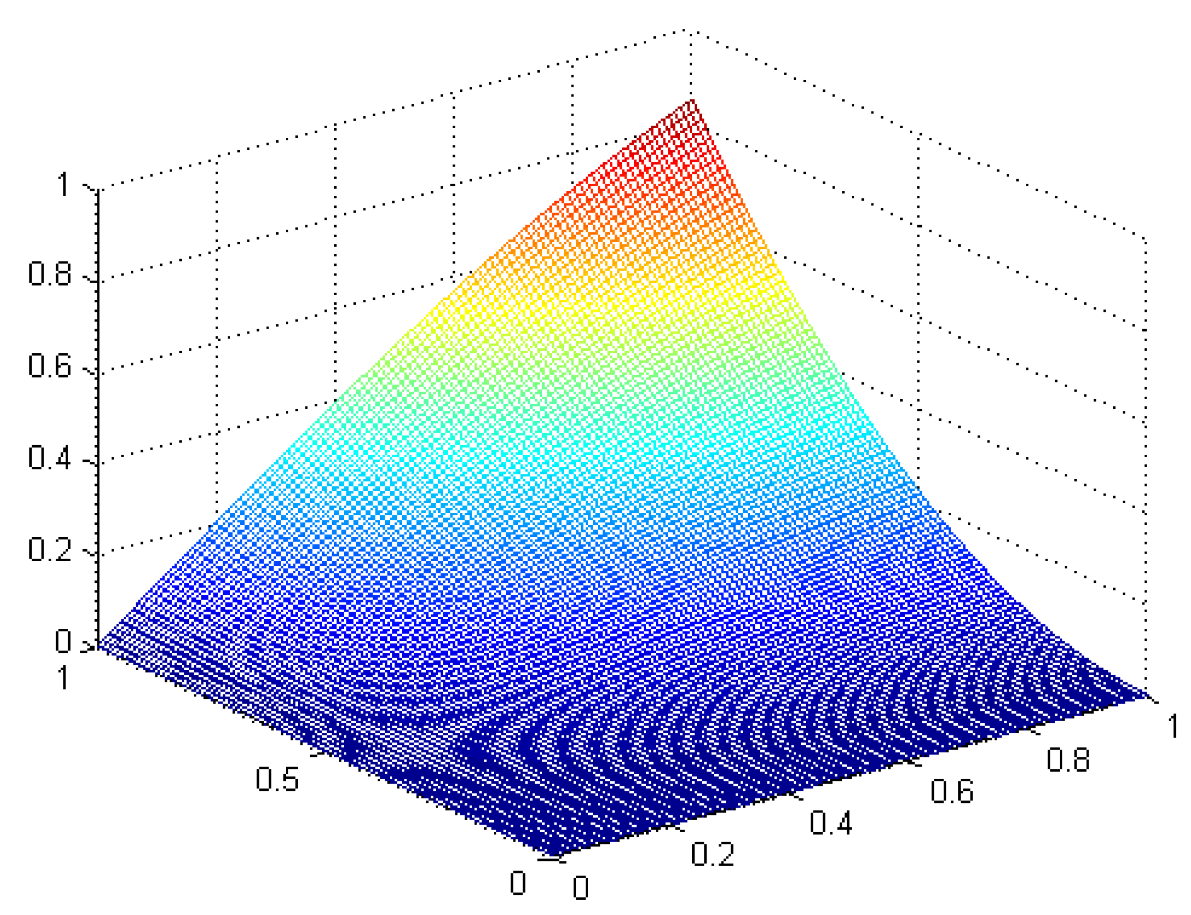
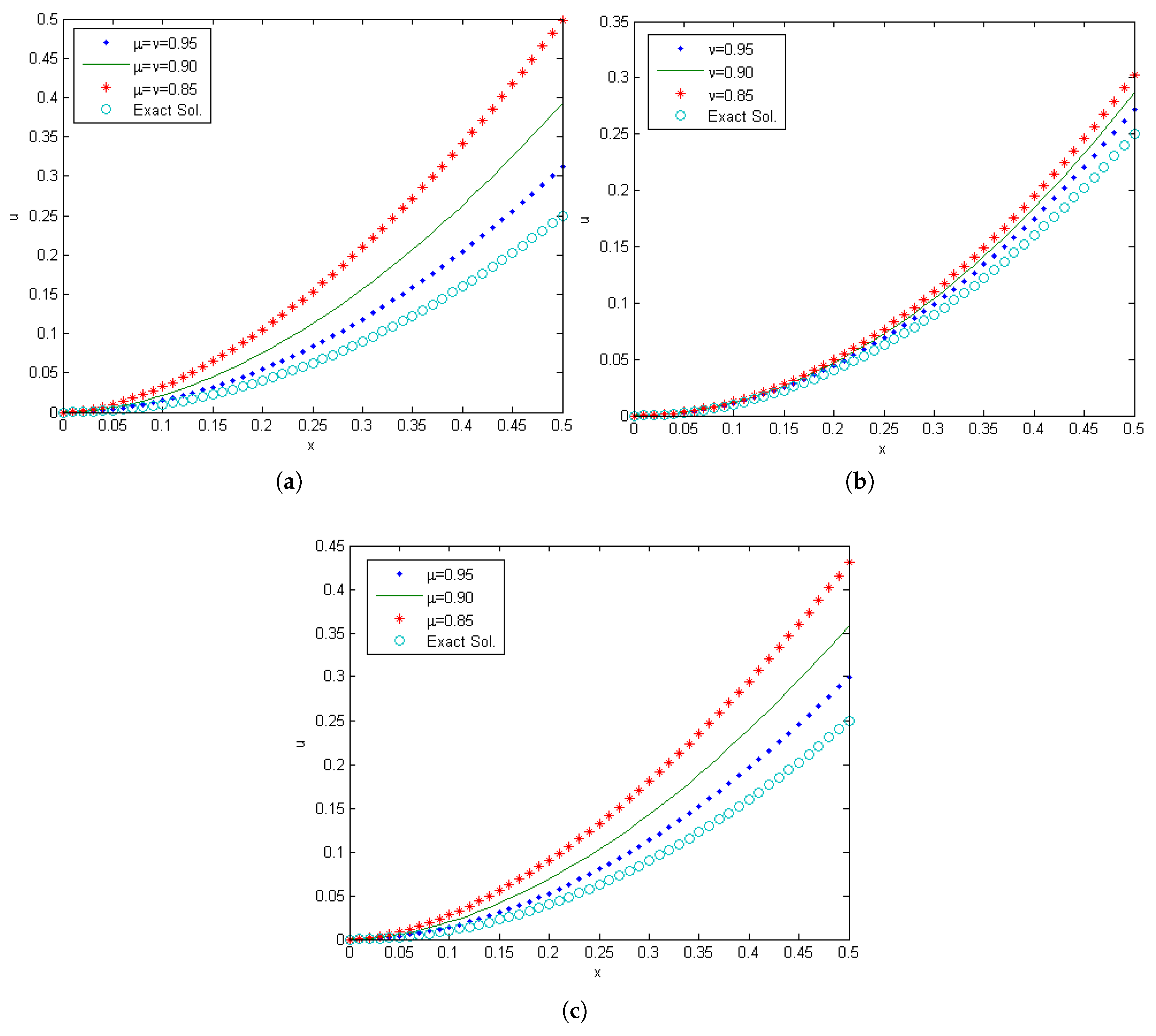
The three dimensional surface in Figure 1 shows the exact solution of Equation (20) in standard form of singular pseudohyperbolic equation at $\mu =\nu =1$. Figure 2 compares the approximate solutions of Equation (20) when $t=\frac{\pi }{2}$. In Figure 2a, the numerical solution at $0<\mu =\nu \le 1$, in this case $u(x,t)$, increases hastily at fractional derivative decrease, Figure 2b shows the solution at $\mu =0.99$ and $\nu =0.95,0.90,0.85$ and we see $u(x,t)$ increasing regularly when $\nu$ decreases, and in Figure 2c we can observe $u(x,t)$ increasing slowly at $\mu =0.95,0.90,0.85$ and $\nu =0.99$ when $\mu$ decreases.

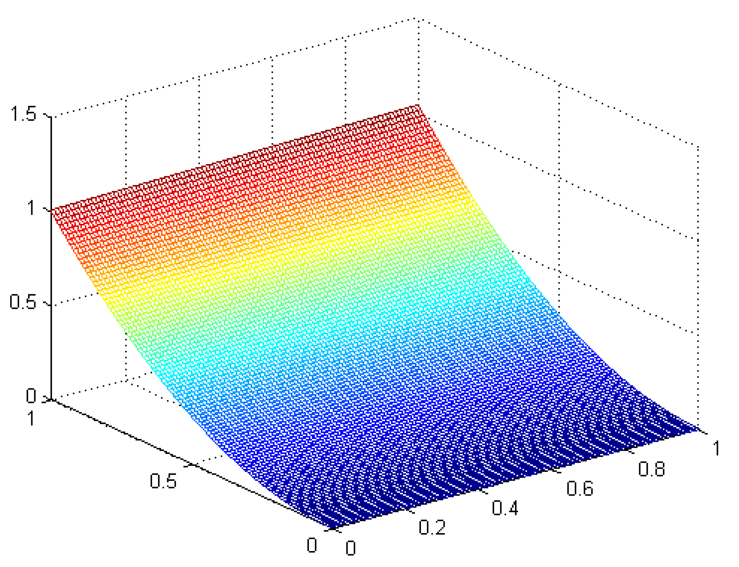
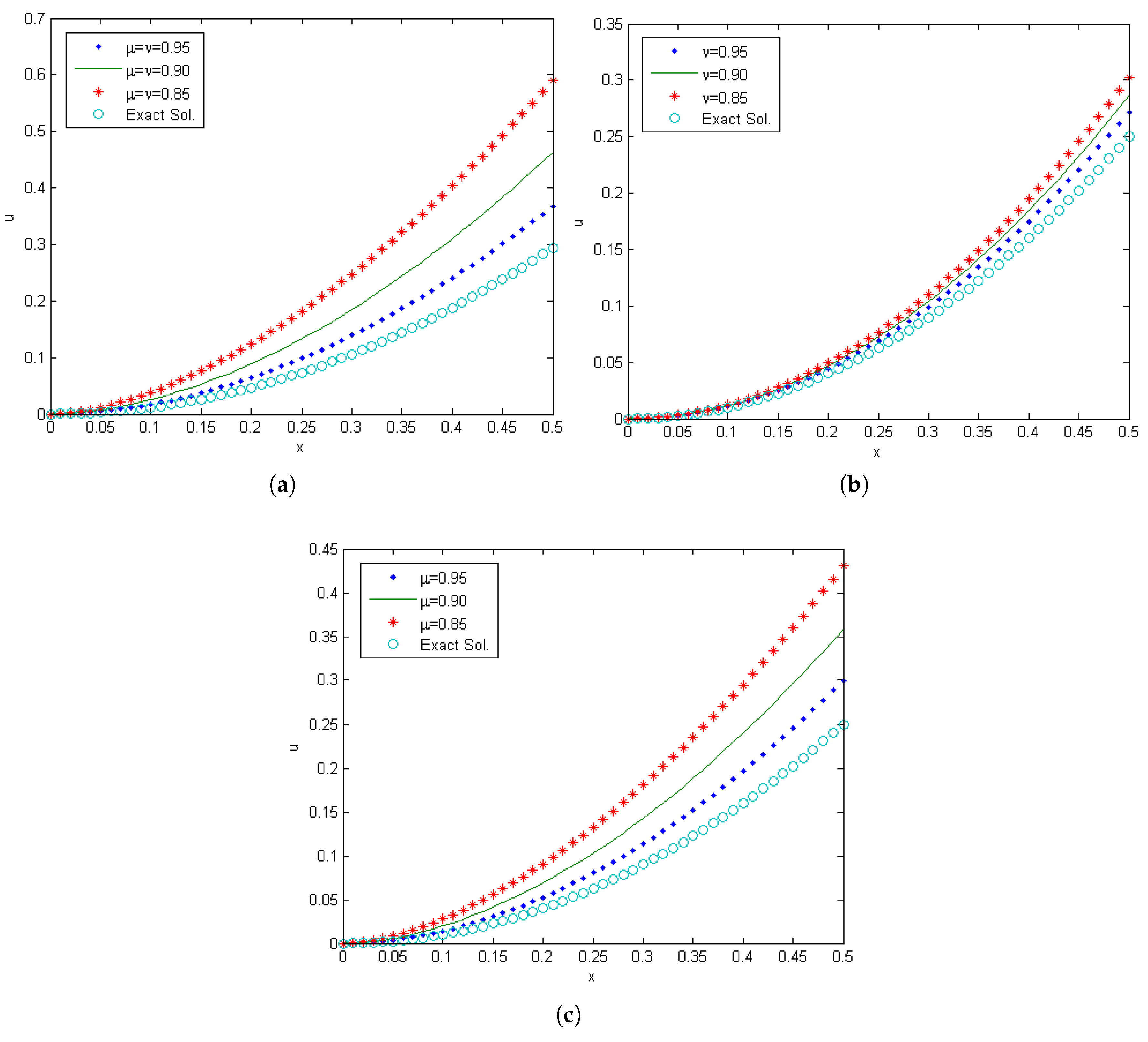
Similarly, the exact solution and approximate solution of Equation (40) were demonstrated in Figure 3 and Figure 4 when $t=1$. In the case $\nu =\mu =1$, we get the exact solution of a singular pseudohyperbolic equation, as seen in Figure 3. Figure 4 shows the approximate solution of Equation (40) with different values of $\mu$ and $\nu$. Figure 4a gives plots of the behavior of Equation (40) when $0<\mu =\nu \le 1$, in this case the function $u(x,t)$ increases quickly, and in Figure 4b we have obtained the solution for the values of $\mu =0.99$ and different values of $0<\nu \le 1$, in this case the function $u(x,t)$ increases gradually, and Figure 4c gives the behavior of Equation (40) at $\nu =0.99$ and different values of $\mu$, in this case the function $u(x,t)$ increasing tardily.

It is clear from the solutions of Equations (20) and (40) that the conformable double Laplace decomposition method has good agreement with the exact solutions of the problems. The fractional-order solution of these two problems and exact solution of integer order problems are equal at $0<\mu =\nu \le 1$, in this case we have no error.

5. Conclusions

In the present work we have studied singular linear and nonlinear pseudohyperbolic equations by employing the conformable double Laplace transform decomposition method (CDLDM), and we obtain analytic solutions when $\mu =\nu =1$ and numerical solutions for different fractional values. Further, we also studied singular coupled pseudohyperbolic equations. It is clear that the solutions of Equations (20) and (40) were obtained as infinite series by using the conformable double Laplace decomposition method and they are in good agreement with the exact solutions of the problems. We have provided three different examples in order to demonstrate the efficiency, high accuracy, and the simplicity of the present method. Further, we plot the exact solutions, as well as the numerical solutions, in Figure 1, Figure 2, Figure 3 and Figure 4, and we can easily see the efficieny of and agreement among the solutions.

References

- Abdelhakim, A.A. The flaw in the conformable calculus: It is conformable because it is not fractional. Fract. Calcul. Appl. Anal. 2019, 22, 242–254. [Google Scholar] [CrossRef]
- Khalil, R.; Al Horani, M.; Yousef, A.; Sababheh, M. A new definition of fractional derivative. J. Comput. Appl. Math. 2014, 264, 65–70. [Google Scholar] [CrossRef]
- Çenesiz, Y.; Baleanu, D.; Kurt, A.; Tasbozan, O. New exact solutions of burgers’ type equations with conformable derivative. Waves Random Complex Media 2017, 27, 103–116. [Google Scholar] [CrossRef]
- Korkmaz, A.; Hosseini, K. Exact solutions of a nonlinear conformable time-fractional parabolic equation with exponential nonlinearity using reliable methods. Opt. Quantum Electron. 2017, 49, 278. [Google Scholar] [CrossRef]
- Ortigueira, M.D.; Machado, J.T. What is a fractional derivative? J. Comput. Phys. 2015, 293, 4–13. [Google Scholar] [CrossRef]
- Aminikhah, H.; Sheikhani, A.R.; Rezazadeh, H. Sub-equation method for the fractional regularized long-wave equations with conformable fractional derivatives. Sci. Iranica Trans. B Mech. Eng. 2016, 23, 1048. [Google Scholar] [CrossRef]
- Chung, W.S. Fractional newton mechanics with conformable fractional derivative. J. Comput. Appl. Math. 2015, 290, 150–158. [Google Scholar] [CrossRef]
- Eslami, M.; Rezazadeh, H. The first integral method for wu–zhang system with conformable time-fractional derivative. Calcolo 2016, 53, 475–485. [Google Scholar] [CrossRef]
- Ünal, E.; Gökdoğan, A. Solution of conformable fractional ordinary differential equations via differential transform method. Optik 2017, 128, 264–273. [Google Scholar] [CrossRef] [Green Version]
- Rahimi, Z.; Rezazadeh, G.; Sumelka, W.; Yang, X. A study of critical point instability of micro and nano beams under a distributed variable-pressure force in the framework of the inhomogeneous non-linear nonlocal theory. Arch. Mech. 2017, 69, 413–433. [Google Scholar]
- Rahimi, Z.; Sumelka, W.; Yang, X.-J. A new fractional nonlocal model and its application in free vibration of timoshenko and euler-bernoulli beams. Eur. Phys. J. Plus 2017, 132, 479. [Google Scholar] [CrossRef]
- Tallafha, A.; Al Hihi, S. Total and directional fractional derivatives. Int. J. Pure Appl. Math. 2016, 107, 1037–1051. [Google Scholar] [CrossRef]
- Hashemi, M. Invariant subspaces admitted by fractional differential equations with conformable derivatives. Chaos Solitons Fractals 2018, 107, 161–169. [Google Scholar] [CrossRef]
- Özkan, O.; Kurt, A. On conformable double laplace transform. Opt. Quantum Electron. 2018, 50, 103. [Google Scholar] [CrossRef]
- Jarad, F.; Abdeljawad, T. A modified laplace transform for certain generalized fractional operators. Results Nonlinear Anal. 2018, 1, 88–98. [Google Scholar]
- Eltayeb, H.; Mesloub, S.; Kılıçman, A. Application of double laplace decomposition method to solve a singular one-dimensional pseudohyperbolic equation. Adv. Mech. Eng. 2017, 9, 1687814017716638. [Google Scholar] [CrossRef]
- Eroğlu, B.; Avcı, D.; Özdemir, N. Optimal control problem for a conformable fractional heat conduction equation. Acta Phys. Pol. A 2017, 132, 658–662. [Google Scholar] [CrossRef]
Figure 1.
The Exact Solutions for Equation (20) when .
Figure 2.
The solutions for Equation (20) for different values of and when . (a) Plot solutions for Equation (20) at . (b) Plot solutions for Equation (20) when and different values of . (c) Plot solutions for Equation (20) for different values of at .
Figure 3.
The Exact Solutions for Equation (40) when .
© 2019 by the authors. Licensee MDPI, Basel, Switzerland. This article is an open access article distributed under the terms and conditions of the Creative Commons Attribution (CC BY) license (http://creativecommons.org/licenses/by/4.0/).
Share and Cite
MDPI and ACS Style
Eltayeb, H.; Mesloub, S.; T. Abdalla, Y.; Kılıçman, A. A Note on Double Conformable Laplace Transform Method and Singular One Dimensional Conformable Pseudohyperbolic Equations. Mathematics 2019, 7, 949. https://doi.org/10.3390/math7100949
AMA Style
Eltayeb H, Mesloub S, T. Abdalla Y, Kılıçman A. A Note on Double Conformable Laplace Transform Method and Singular One Dimensional Conformable Pseudohyperbolic Equations. Mathematics. 2019; 7(10):949. https://doi.org/10.3390/math7100949
Chicago/Turabian StyleEltayeb, Hassan, Said Mesloub, Yahya T. Abdalla, and Adem Kılıçman. 2019. "A Note on Double Conformable Laplace Transform Method and Singular One Dimensional Conformable Pseudohyperbolic Equations" Mathematics 7, no. 10: 949. https://doi.org/10.3390/math7100949
Note that from the first issue of 2016, this journal uses article numbers instead of page numbers. See further details here.