Optimization of Energy Storage Operation Chart of Cascade Reservoirs with Multi-Year Regulating Reservoir

Abstract

In view of the problems that have not been solved or studied in the previous studies of cascade Energy Storage Operation Chart (ESOC), based on a brief description of the composition, principle, drawing methods, and simulation methods of ESOC, the following innovative work has been done in this paper. Firstly, considering the inconsistency of inflow frequency of upstream and downstream watershed in selecting the typical dry years, a novel optimization model for selecting the overall inflow process considering the integrity of watershed was proposed, which aimed at minimizing the sum of squares of inflow frequency differences. Secondly, aiming at the influence of output coefficients (including number and values) on the results of ESOC, this paper proposed a new method to construct the initial solution of output coefficients and established an optimization model of output coefficients based on progressive optimality algorithms. Thirdly, to the optimization of ESOC with multi-year regulating reservoir, a discrete optimization model of drawdown level was constructed based on the idea of ergodic optimization. On these bases, taking the seven reservoirs in the Yalong River basin of China as an example, the typical dry years considering the inflow frequency inconsistency, the optimal output coefficients of ESOC and the optimal end-of-year drawdown level of a multi-year regulating reservoir (Lianghekou) were obtained, and compared with the previous research results, the ESOC optimized in this paper can increase the total power generation of the cascade system by 9% under the condition that the guaranteed rate did not change much. Furthermore, the difference of the optimal end-of-year drawdown levels between the cascade joint operation and single reservoir operation was discussed for the Lianghekou reservoir at the end of the case study. The obtained results were of great significance for guiding the actual operation of cascade reservoirs.

1. Introduction

As a renewable and clean energy [1,2], hydropower energy is a kind of high quality and efficient energy which is being vigorously developed all over the world [3]. Its development and utilization is mainly through the construction of reservoirs to concentrate and raise water head, so that the water energy can be efficiently converted into electricity. In recent years, with the construction and operation of various types of reservoirs, cascade reservoirs with the water quantity and water head connections of upstream and downstream have gradually formed [4,5].

After the formation of cascade reservoirs, the original single reservoir operation method can no longer meet the needs of the joint operation of cascade reservoir [6,7]. Therefore, it is necessary to develop and study new joint operation methods, including optimization methods and conventional methods [8,9], the optimal operation methods include classical mathematical methods and intelligent clustering algorithms [10]. Linear programming [11] and dynamic programming [12,13,14], etc. belong to classical mathematical methods. Genetic algorithms [15,16,17] and particle swarm optimization [18,19,20], etc. belong to intelligent clustering algorithms [21]. Conventional operation methods include operation functions, operation rules, and operation charts [22,23]. In the conventional operation method of single reservoir, the most common one is the operation chart. After the cascade reservoirs have been formed by many reservoirs, the corresponding conventional joint operation method is the cascade joint operation chart, such as Energy Storage Operation Chart (ESOC).

At present, there are some literatures about the drawing, application, and optimization of cascade joint operation charts or rules, and some advancements have been achieved. For example, using dynamic programming and non-dominated sorting genetic algorithm-II, Liu et al. [24] derived the joint operating curves for cascade hydropower reservoirs of China’s Qing River, which are better than linear operating rules. Ostadrahimi et al. [25] presented and tested a set of operation rules for a multi-reservoir system, employing a multi-swarm version of particle swarm optimization (MSPSO) in connection with the well-known HEC-ResPRM simulation model in a parameterization-simulation-optimization (parameterization SO) approach. Taghian et al. [26] developed a hybrid model to optimize simultaneously both the conventional rule curve and the hedging rule for a multipurpose, multireservoir system in southern Iran, and in the compound model, a simple genetic algorithm was coupled with a simulation program, including an inner linear programming algorithm. Bolouri-Yazdeli et al. [27] addressed the application of real-time operation rules on a reservoir system whose purpose is to supply total downstream demand, including standard operation policy, stochastic dynamic programming, linear decision rules, and nonlinear decision rule (NLDR) with various orders of inflow and reservoir storage volume. Li et al. [28] derived the explicit nonlinear formulation of operating rules for multi-reservoir using the genetic programming, and found that the results were more efficient and reliable than artificial neural network rules. Aboutalebi et al. [29] proposed a novel tool that couples the nondominated sorting genetic algorithm (NSGAII) with support vector regression (SVR) and nonlinear programming (NLP) to optimize monthly operation rules for hydropower generation, and the evaluation results indicate that the SVR-NSGAII is well suited to calculate the optimal hydropower reservoir operation rule in real time. Jiang et al. [30] proposed three key technologies in the drawing process and one key technology in the practical application of ESOC, several difficult problems in drawing and application of ESOC are solved, and realized the combined utilization of DCM and ESOC. Ashrafi and Dariane [31] proposed an effective improved Melody Search (IMeS) algorithm to achieve the optimal operating rules of multi-reservoir systems with local demands, and the efficiency of the optimization method was compared to the results achieved by other selected well-known heuristic search methods, and revealed that the proposed algorithm is more effective in finding precise solutions over a long-term period. Aimed at the defects of the conventional two-stage Progressive Optimality Algorithm (POA) in the optimization of ESOC, Jiang et al. [32] proposed a new multi-stage POA optimization model which took the traditional reverse calculation result as the initial solution, and expanded the two-stage optimization mode of conventional POA to higher stages mode, and this research realized the effective optimization of ESOC by the improved POA. Jiang et al. [33] studied the drawing method of ESOC and its simulation operation processes, and through the study of ESOCs under different time scales of operation stage (5d, 10d, 15d, 20d, 30d, and 60d), the influence law of operation stage length on power generation is analyzed and discussed. Jiang et al. [34] improved and expanded the traditional ESOC model for pure cascade reservoirs based on the special relationships between the upstream and downstream reservoirs in a mixed reservoir system, and considering the objectives of flood control, energy generation, and ecological flow, a multi-objective ESOC optimization model for large-scale mixed reservoirs was established.

However, in the above researches, although many achievements have been made in the drawing, simulation application, and optimization of ESOC, several problems have not been taken into account. Firstly, there is no specific method for choosing a typical dry year. Especially for the inconsistency of inflow frequencies of upstream and downstream, there is no relevant research and discussion, which is very prominent when the basin area is large. Secondly, the optimization of output coefficients has not been considered in detail. Although the optimization of output coefficients has been studied in the literature by Jiang et al. [30], it did not put forward a complete optimization idea or optimization process. Thirdly, for the cascade reservoir system with multi-year regulating reservoirs, the end-of-year drawdown level of multi-year regulating reservoirs should be taken into account. However, previous studies did not involve the multi-year regulating reservoirs.

In view of this, on the basis of previous studies, aiming at the unsolved or unstudied problems, taking the cascade system of 7 reservoirs in the Yalong River basin as an example, this paper specifically studies the optimal selection of typical dry years considering the inflow frequencies inconsistency of upstream and downstream, the optimization of the output coefficients of ESOC, and the optimization of ESOC for cascade reservoirs with multi-year regulating reservoir. The goals are to further improve the related research of ESOC on the basis of the previous researches and promote the development of joint optimal operation of cascade reservoirs.

2. Methodology

2.1. Drawing and Simulation of ESOC

ESOC is a commonly used medium- and long-term joint dispatching method for cascade reservoirs, which consists of two basic operation curves, several increased and reduced output curves. These output curves divide the ESOC into several output zones, including the guaranteed output zone, the increased output zones, and the reduced output zones. ESOCs are usually obtained by an inverse regulation calculation using the typical runoff of dry years. In order to distribute the total output of cascade system to each power station in the drawing process, the discriminant coefficient method is used.

Maximizing the power generation and minimizing the energy loss by determining the best order of reservoirs in storing water or supplying water is the principle of discriminant coefficient method. The optimal order of water storage or water supply for cascade reservoirs can be calculated by the following formula.

$$K_t^i==\left(0.5W_t^i+{\displaystyle \sum _{j=0}^{i-1}{V}_{avai,t}^j}\right)/\left(A_t^i\cdot {\displaystyle \sum _{j=i}^n{H}_t^j}\right)$$

(1)

where K_tⁱ is the discriminant coefficient of the ith reservoir in the tth stage; i is the index of reservoir; t is the index of operation stage; W_tⁱ is the natural inflow water of the ith reservoir in the tth stage; V^j_avai,t is the available water of the jth reservoir in the tth stage; A_tⁱ is average water surface area of the ith reservoir in the tth stage; Hⁱ_t is average water level of the ith reservoir in the tth stage; n is the total number of reservoirs in the cascade system, reservoirs are numbered 0, 1, 2, …, n from upstream to downstream.

In general, if the cascade system is going to store water, the best reservoir for water storage is the one that has the maximum Kⁱ_t. Similarly, if the cascade system is going to supply water, the best reservoir for water supply is the one that has the minimum Kⁱ_t. The detailed analysis and derivation about this formula can be found in literatures by Jiang et al. [30].

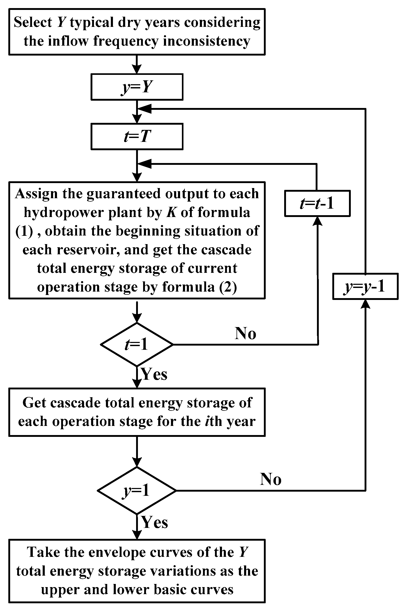
As mentioned earlier, the ESOC mainly includes the basic operation curves, the increased and the reduced output curves. Specifically, assuming that a total of Y typical dry years are selected through the method of the following Section 2.2, the details of drawing the upper and lower basic output curves can be shown in Figure 1 [33], in which the y is the index of typical year, T is the total number of operation stages, and t is the index of operation stage. In addition, considering the output coefficients optimization of ESOC described in Section 2.3, the details of drawing the increased and reduced output curves can be shown in Figure 2 [33].

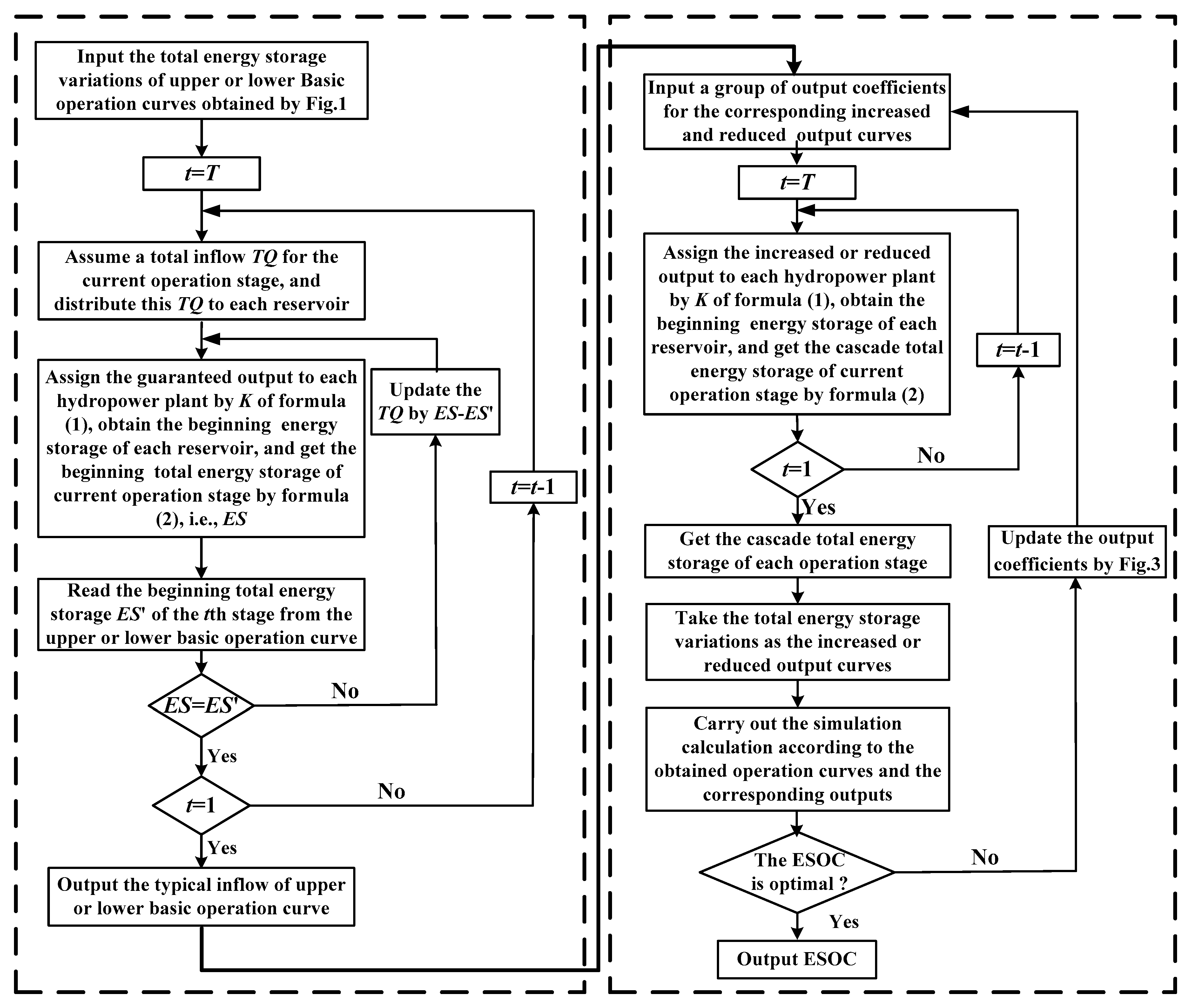
In Figure 2, the total energy storage ES_t of the cascade system is calculated by Formula (2), where γ is the specific gravity of water and ESⁱ_t is the energy storage of ith reservoir in the tth stage. The meanings of other variables in Formula (2) are the same as Formula (1).

$${{\displaystyle ES}}_t={\displaystyle \sum _{i=1}^n{{\displaystyle ES}}_t^i}=\gamma {\displaystyle \sum _{i=1}^n\left({{\displaystyle V}}_{\mathrm{avai},t}^i\cdot {\displaystyle \sum _{j=i}^n{{\displaystyle H}}_t^j}\right)}$$

(2)

After obtaining the ESOC, the simulation calculation is usually carried out using the long series of runoff data, to obtain the annual average power generation and guaranteed rate and other indicators. The simulation processes can be described as follows:

Firstly, calculate the total energy storage ES_t of the cascade system by Formula (2). Secondly, get an output from ESOC by ES_t, suppose its TL_t,chart, and calculate the total output of cascade system by natural inflow, suppose its TL_t,inflow. Thirdly, according to the relationship between TL_t,inflow and TL_t,chart, judging whether the cascade system is going to store water or supply water, and the corresponding operation can be carried out in the following three situations.

(1)

If TL_t,inflow > TL_t,chart, then the cascade system is going to store water, the reservoir that has maximum Kⁱ_t begins to store water first, until the calculated total output is equal to TL_t,chart. If this reservoir is filled up and the output has not yet reached TL_t,chart, then the reservoir that has the second largest Kⁱ_t begins to store water.

(2)

If TL_t,chart > TL_t,inflow, then the cascade system is going to supply water, the reservoir that has minimum Kⁱ_t begins to supply water first, until the calculated total output is equal to TL_t,chart. If this reservoir is emptied and the output has not yet reached TL_t,chart, then the reservoir that has the second smallest Kⁱ_t begins to supply water.

(3)

If TL_t,chart = TL_t,inflow, then there is no water supply or water storage, thus the system produces hydropower by natural inflow only.

More detailed description on the drawing and simulation of ESOC based on DCM can be found in the literatures by Jiang et al. [30,33]. In the above-mentioned drawing process of ESOCs, there are the following difficulties. (1) Selection of typical dry years considering the whole basin. (2) Determination of the number and output values of the increased and reduced output curves, that is, the optimization of the output coefficients of ESOC. (3) If there are multi-year regulating reservoirs in the cascade system, the drawdown level of the multi-year regulating reservoirs should also be considered.

2.2. Selection of Typical Dry Years Considering the Inflow Frequency Inconsistency

An important input in drawing ESOC is the typical runoff of dry years. Therefore, in order to get a reasonable ESOC, it is necessary to select a set of runoff processes of typical dry years, and try to make the inflow frequency of upstream and downstream consistent or not much different. In fact, when the basin area is large, the inflow frequency of upstream and downstream stations is often inconsistent at the same time. For example, when the inflow frequency of upstream station is 70%, the inflow frequency of downstream station at the same time may be 50%, which causes the inflow frequency inconsistency of upstream and downstream stations. In practical applications, it is very difficult or even impossible to make the inflow frequency of upstream and downstream stations exactly the same. The drawing of ESOC is based on the whole river basin, so how to consider the inflow frequency inconsistency of different stations in selecting the typical dry years is the key to getting reasonable ESOC.

According to the conventional method, the total annual runoff of each station can be obtained by summing up the ten-day or monthly runoff of each year, and then the empirical inflow frequency of each station can be obtained by calculating the frequency of the total annual runoff. The empirical frequency formula is shown in Formula (3).

$$P=m/(M+1)$$

(3)

where m is the corresponding index number of the year after the total annual runoff is sorted by descending order, and M is the total number of hydrological years.

After getting the results of the inflow frequency of each station, it is necessary to calculate the overall inflow frequency of the whole river basin. Because the upstream and downstream inflow frequencies are usually not consistent in the same year in a river basin, it is impossible to find an overall inflow process that is fully consistent with the inflow frequencies of upstream and downstream. We can only find an overall inflow process with the smallest difference between the upstream and downstream inflow frequencies.

Specifically, set i as the index number of hydropower stationand y as the index number of hydrological years. The actual inflow frequency of each station in the yth year is P_i^y, which is obtained by its own frequency arrangement. If we want to get the optimal inflow process of the whole basin under a certain frequency P_s, it is equivalent to calculating the y corresponding to the smallest e_y, which is shown in Formula (4).

$$e_y^s={\displaystyle \sum _{i=1}^n{(p_s-p_i^y)}^2},y=1,2,\dots ,Y$$

(4)

The above method is to deduce the best inflow process of the whole basin corresponding to the specific frequency P_s (a year). Conversely, a similar method can be used to derive the overall inflow frequency of each year for the river basin, such as the actual inflow frequency of the whole river basin in the y year. The steps are as follows.

Step1:

Discretize the possible range of inflow frequency into S discretized values, and get P₁, P₂, …, P_S.

Step2:

Obtain the corresponding P_i^y (I = 1, 2, …, n) of each station according to the actual inflow in the y year of the basin.

Step3:

For each Ps (s = 1, 2, …, S), calculate the e^s_y (s = 1, 2, …, S) by formula (4).

Step4:

Obtain the actual inflow frequency Ps^* of the whole basin in y year by finding the s that corresponds to the minimum e^s_y.

Through the above steps, the overall inflow frequency of each year of the whole basin can be obtained, from which the typical runoff processes of dry years can be selected to draw the ESOC.

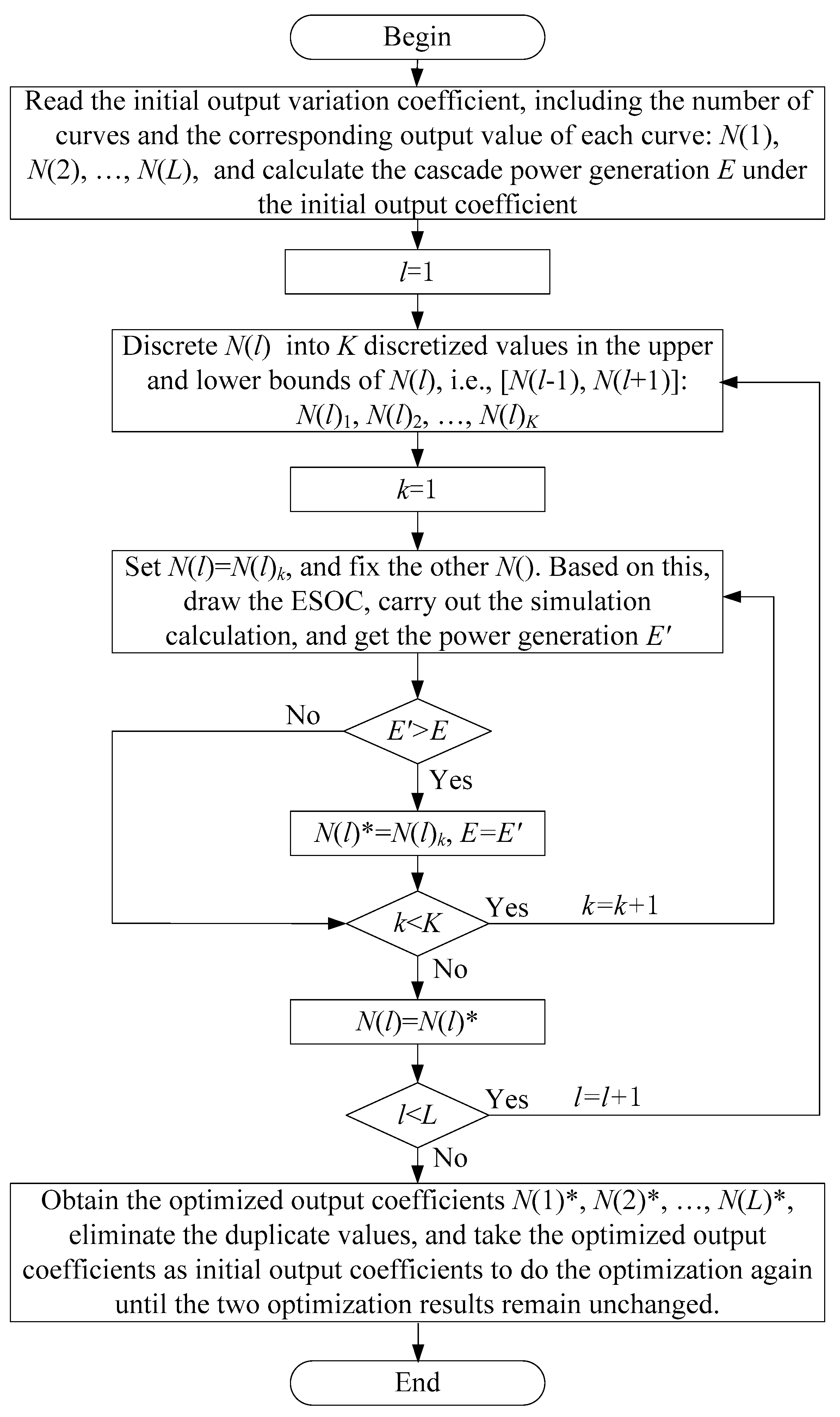
2.3. Optimization of Output Coefficients for Energy Storage Operation Chart

One of the difficulties in drawing the ESOC is to determine the reasonable output coefficients, which has a direct impact on the output of each stage of ESOC in the application. The determination of output coefficients includes two aspects. One is the determination of the number of output coefficients, and the other is the determination of the value of each output curve.

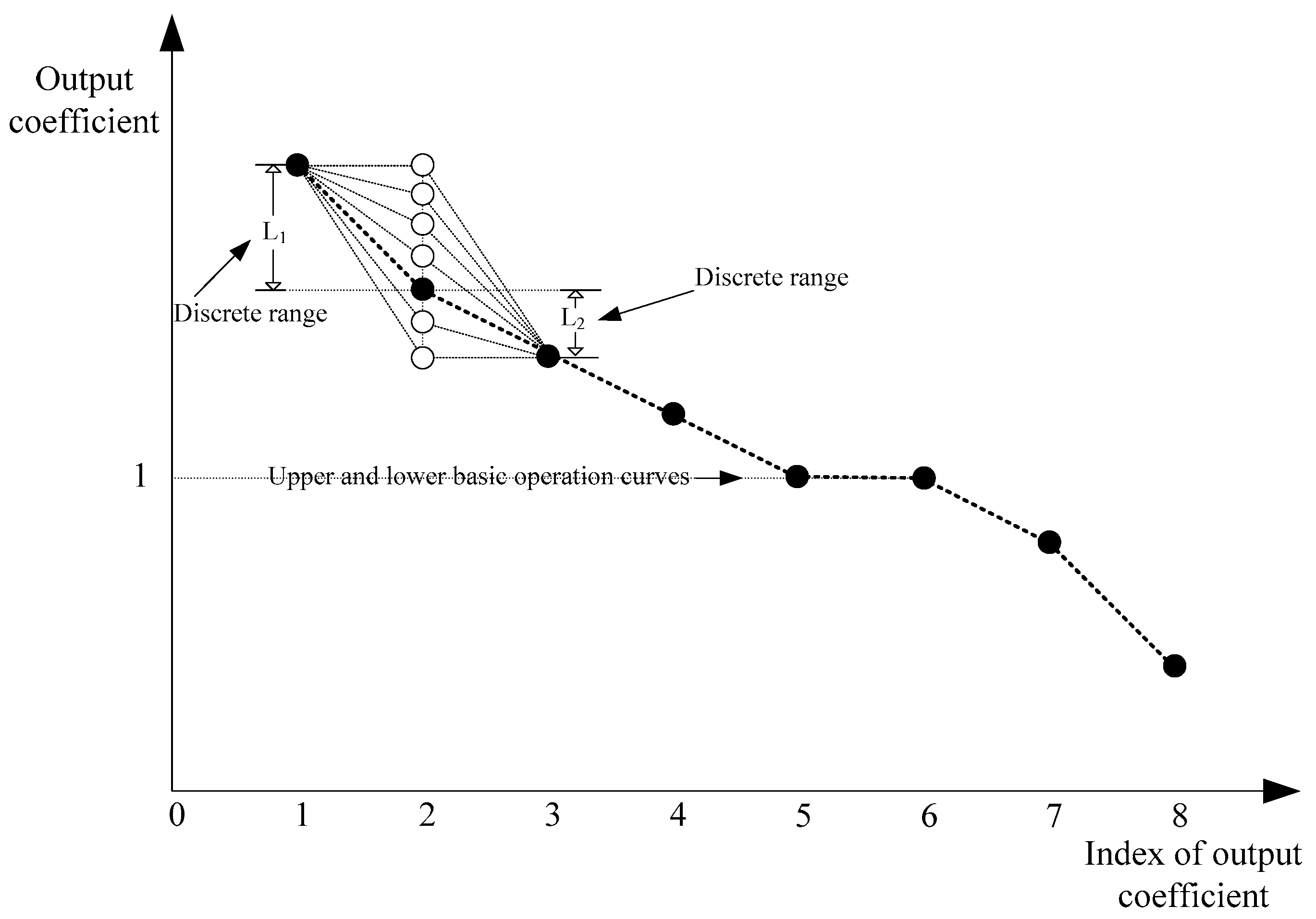
In order to determine the reasonable output coefficients of ESOC, this paper adopts the POA to optimize the output coefficients. The idea is to get an initial solution (including the number of curves and the value of each curve) within the feasible range, and then use POA to optimize it [35,36]. In an optimization process, when a point is optimized, its discrete range is the corresponding range of former point and latter point. In the optimization, we divide the range uniformly into a series of discrete points, and simulate each discrete point under the condition that other output coefficients remain unchanged, so as to obtain the corresponding power generation, and finally select the discrete point corresponding to the maximum power generation by comparison [37]. The distance between these two discrete points is called a discrete interval. The optimization diagram is shown in Figure 3. In the process of optimization, the number of output coefficients and the corresponding values are updated step by step, and finally the optimal output coefficients can be obtained.

In the above-mentioned method, the updating of the number of output coefficients mainly means that, for two or several coefficients which are identical or very close to each other after a certain optimization, only one of them can be selected and retained. So it is equivalent to optimizing the number of output curves.

In order to avoid the influence of initial solutions on the results, we constructed an initial solution generation method based on the characteristics of output coefficients and their possible upper and lower limits. The characteristics of output coefficients are as follows:

(1)

In the output coefficients, there are two points equal to 1, which correspond to the basic operation curves, i.e., guaranteed output zone. This is a fixed value.

(2)

In order to avoid the intersection of output curves, the output coefficient decreases in turn (or increases in turn), i.e., two adjacent output values are separated by at least one discrete interval.

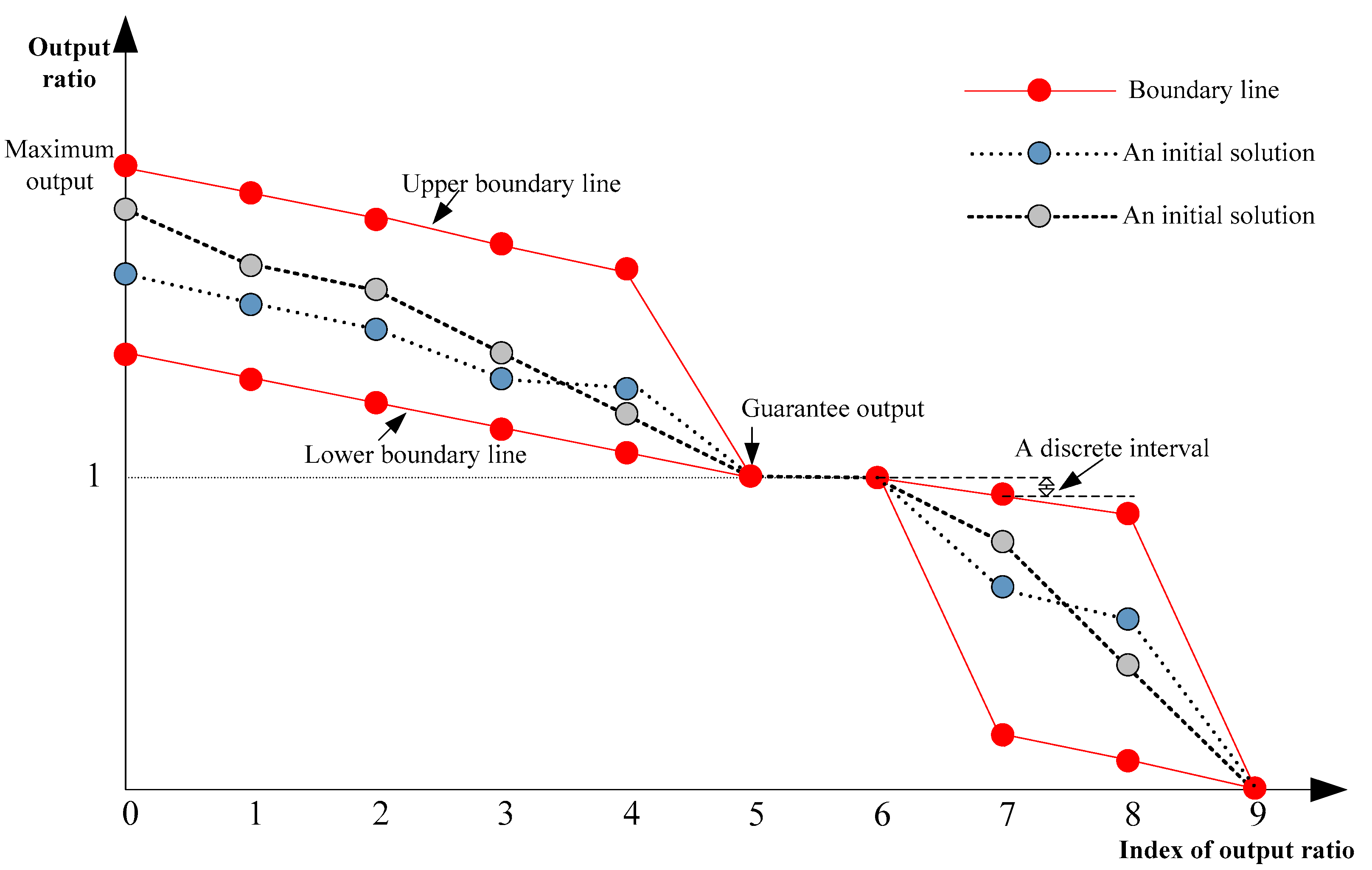
Through the above characteristics, the possible space of the initial solution can be obtained, as shown in Figure 4, where the red dot line represents the upper and lower bounds of the output coefficients. Two horizontal points represent the upper and lower basic operation curves. The gray and light blue dot lines represent an initial solution within the allowable range, respectively. In order to avoid the intersection of the operation curves, the upper boundary line decreases gradually with a discrete interval at the maximum output coefficient in the increased output zone and at the output coefficient of the lower basic operation curve in the reduced output zone. Similarly, the lower boundary line increases gradually with a discrete interval at the output coefficient of the upper basic operation curve in the increased output zone and at the zero value point in the reduced output zone. As can be seen from Figure 4, the determination of the upper and lower bounds only needs to determine the maximum output and the size of a discrete interval.

The steps to construct an initial solution are as follows:

Step 1:

For the first point, randomly generate a value within the upper and lower boundary of the output coefficient to form the first point N(1).

Step 2:

For the second point of the output coefficient, randomly generate a value in the interval [Lower, N(1)] to form the second point N(2).

Step 3:

Similarly, for the lth point, randomly generate a value in the interval [N(l-1), Lower] to form the lth point N(l).

Step 4:

Repeat step 3 to get an initial solution N(1), N(2), …, N(l), …, N(L).

For an initial solution, the whole process of output coefficients optimization can be represented by Figure 5.

2.4. Optimization of Drawdown Level for Multi-Year Regulating Reservoir

In the previous studies of ESOC, the reservoirs involved are mainly the annual or seasonal regulating reservoirs, and the multi-year regulating reservoirs are not involved. After the multi-year regulating reservoirs involved, the situation will be changed. This is because, generally speaking, in the single reservoir operation, the water level of multi-year regulating reservoirs will not be drawn down to a dead level at the end of the year, as there is a need to retain a part of the water for usage in later years. Therefore, the end-of-year drawdown level of the reservoir should be taken into account when the multi-year regulating reservoir is involved in the process of drawing the ESOC.

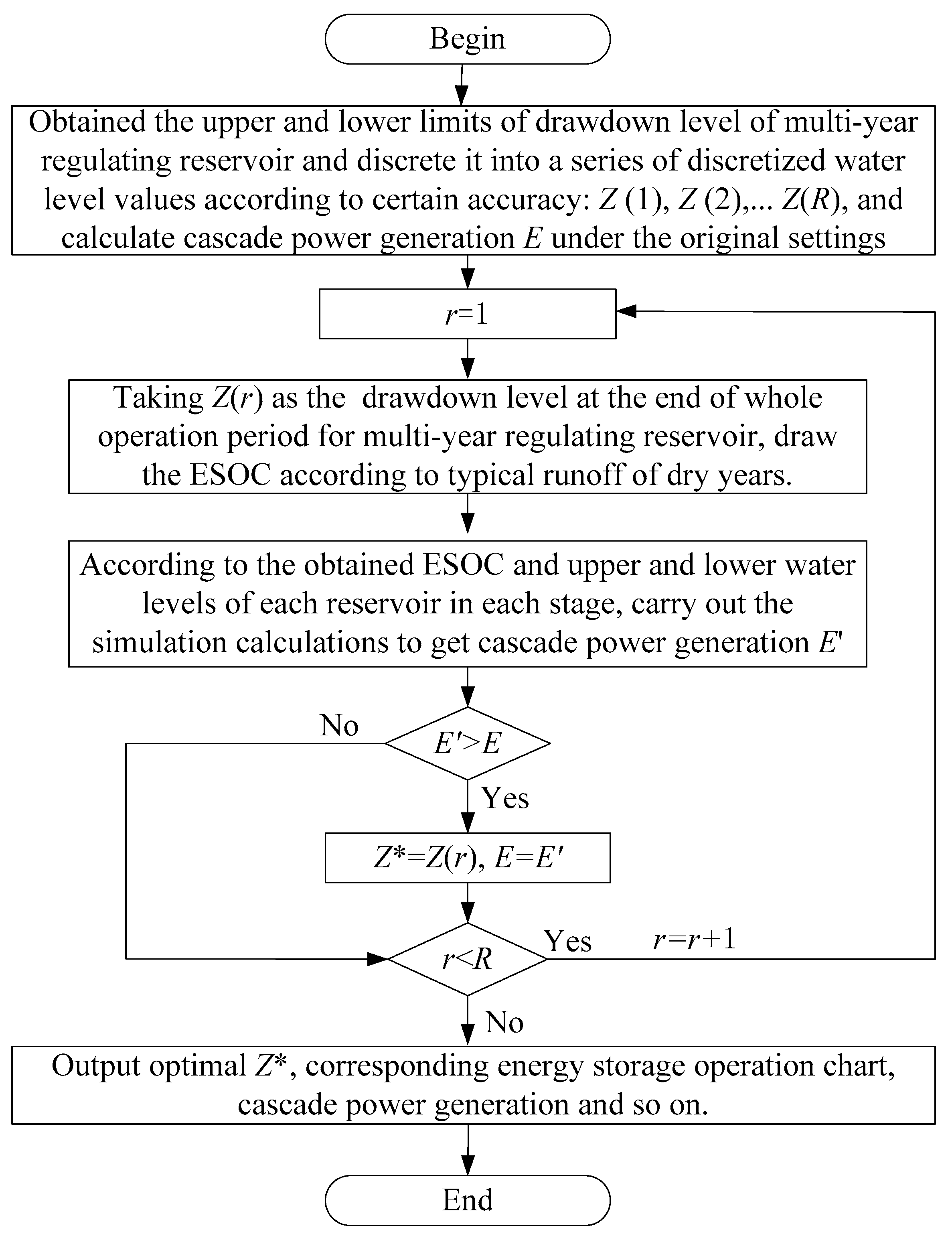
In order to determine the optimum drawdown level, we can firstly determine a series of discrete values of the drawdown level according to the possible range of the water level at the end of the year, and then draw the corresponding ESOC for each level, and carry out the simulation operation and get the power generation, and select the optimum drawdown level according to the total power generation of cascade system at last. The specific implementation process can be shown in Figure 6.

3. Case Study

3.1. Basin Introduction and Basic Data

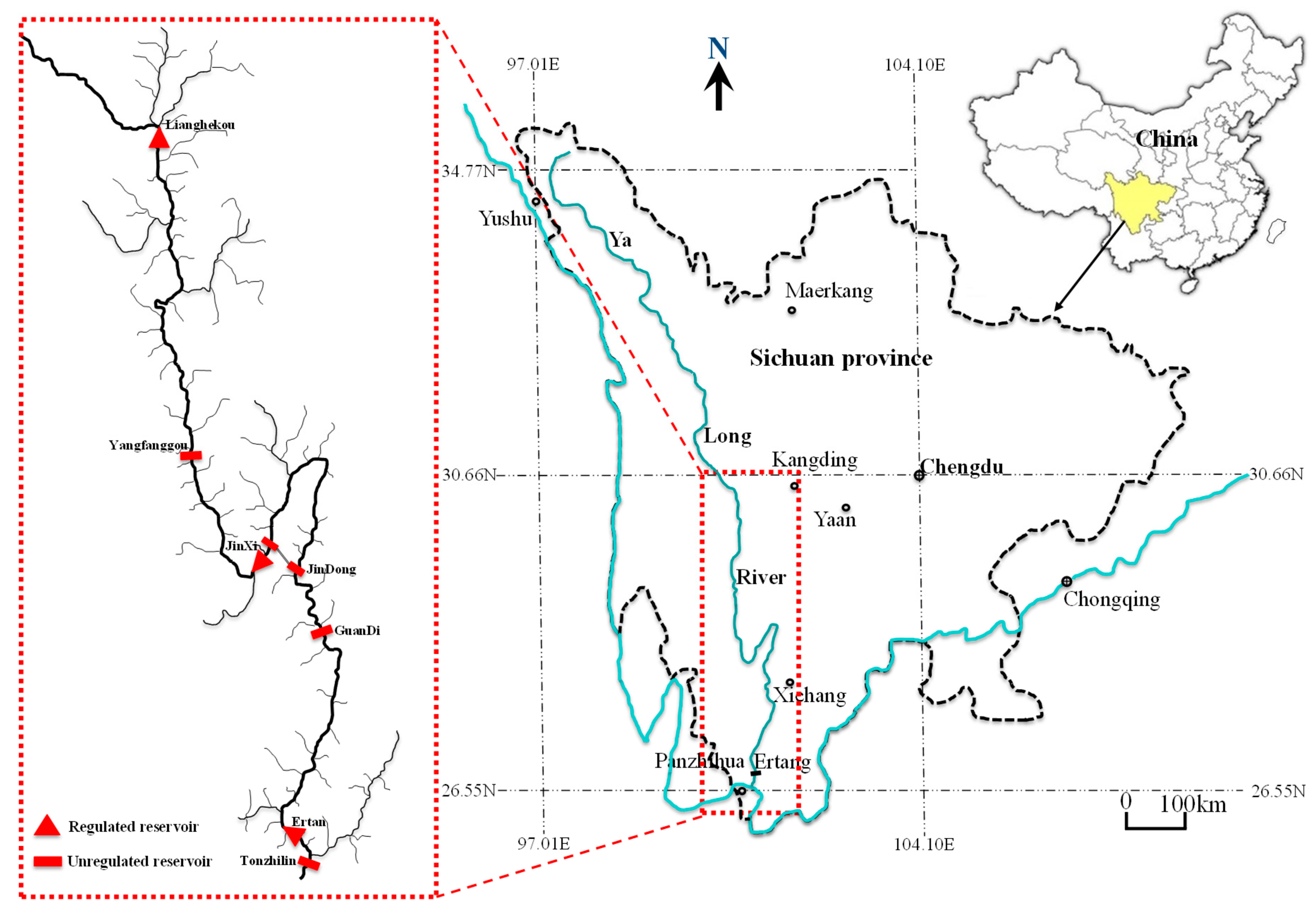
Yalong River, the largest tributary of Jinsha River, originated in Yushu County, Qinghai Province. The whole length of the main river is 1571 km, the area of the basin is about 136,000 km², and the natural drop is about 3830 m. The average annual flow at the estuary is 1910 m³/s, with an annual runoff volume of nearly 60 billion m³, accounting for 13.3% of the total water in the upper reaches of the Yangtze River. Yalong River has abundant water resources, and a total of 22 hydropower stations are planned in the main stream, with a total installed capacity of about 30 million kWh and an annual power generation of about 150 billion kWh.

At present, there are seven hydropower stations in the Yalong River basin, including Lianghekou, Yangfanggou, Jinxi, Jindong, Guandi, Ertan, and Tongzilin. Among them, Lianghekou, Jinxi, and Ertan are the three reservoirs with regulating performance, and the Lianghekou is a multi-year regulating reservoir. Their geographical locations are shown in Figure 7.

In this case, the seven reservoirs mentioned above are taken as the research object, and the ESOC including multi-year regulating reservoir is studied. Some basic parameters of each reservoir are shown in

Table 1. Some basic parameters of the cascade reservoirs.

Item	Unit	Lianghekou	Yangfanggou	Jinxi	Jindong	Guandi	Ertan	Tongzilin
Normal level	m	2865	2088	1880	1646	1330	1200	1015
Dead level	m	2785	2094	1800	1640	1321	1155	1010
Flood control level	m	2845.9	none	1859	none	none	1190	none
Regulation performance	---	Multi-year	Daily	Annual	Daily	Daily	Seasonal	Daily
Installed capacity	MW	3000	1500	3600	4800	2400	3300	600
Guaranteed output	MW	1130	253	1086	1443	709.8	1028	227
Range of operating water level	m	[2845.9, 2865] or [2785, 2865]	2092	[1859, 1880] or [1800, 1880]	1644	1328	[1155, 1200] or [1190, 1200]	1013.5

.

3.2. Results and Discussion

3.2.1. Typical Dry Years Selection

At present, we have a ten-day runoff series from June 1957 to May 2019, a total of 62 years, which means M = 62 in the Formula (3). According to Formula (3), the corresponding inflow frequencies for each hydrological year of each station are shown in

Table 2. Inflow frequency of each station in each hydrological year.

Year	Lianghekou	Jingxi	Ertan	Year	Lianghekou	Jingxi	Ertan
1957–1958	25.4%	17.5%	6.3%	1988–1989	66.7%	58.7%	58.7%
1958–1959	85.7%	69.8%	57.1%	1989–1990	14.3%	20.6%	23.8%
1959–1960	92.1%	90.5%	88.9%	1990–1991	31.7%	22.2%	20.6%
1960–1961	19.0%	23.8%	27.0%	1991–1992	47.6%	28.6%	11.1%
1961–1962	71.4%	79.4%	81.0%	1992–1993	76.2%	77.8%	76.2%
1962–1963	27.0%	19.0%	15.9%	1993–1994	7.9%	4.8%	9.5%
1963–1964	15.9%	33.3%	39.7%	1994–1995	93.7%	95.2%	93.7%
1964–1965	46.0%	34.9%	34.9%	1995–1996	73.0%	55.6%	54.0%
1965–1966	1.6%	1.6%	1.6%	1996–1997	55.6%	41.3%	49.2%
1966–1967	38.1%	30.2%	14.3%	1997–1998	82.5%	66.7%	69.8%
1967–1968	74.6%	82.5%	90.5%	1998–1999	23.8%	3.2%	3.2%
1968–1969	61.9%	42.9%	31.7%	1999–2000	20.6%	15.9%	7.9%
1969–1970	77.8%	74.6%	74.6%	2000–2001	12.7%	14.3%	30.2%
1970–1971	52.4%	50.8%	44.4%	2001–2002	49.2%	31.7%	28.6%
1971–1972	81.0%	84.1%	71.4%	2002–2003	96.8%	73.0%	82.5%
1972–1973	69.8%	92.1%	85.7%	2003–2004	11.1%	7.9%	19.0%
1973–1974	98.4%	98.4%	92.1%	2004–2005	28.6%	25.4%	36.5%
1974–1975	36.5%	12.7%	4.8%	2005–2006	6.3%	9.5%	33.3%
1975–1976	58.7%	81.0%	77.8%	2006–2007	90.5%	93.7%	96.8%
1976–1977	44.4%	65.1%	66.7%	2007–2008	87.3%	76.2%	87.3%
1977–1978	63.5%	63.5%	65.1%	2008–2009	54.0%	39.7%	42.9%
1978–1979	79.4%	60.3%	47.6%	2009–2010	30.2%	44.4%	52.4%
1979–1980	42.9%	71.4%	55.6%	2010–2011	68.3%	57.1%	68.3%
1980–1981	17.5%	38.1%	25.4%	2011–2012	65.1%	88.9%	98.4%
1981–1982	60.3%	61.9%	50.8%	2012–2013	3.2%	6.3%	12.7%
1982–1983	33.3%	47.6%	46.0%	2013–2014	50.8%	68.3%	73.0%
1983–1984	88.9%	96.8%	95.2%	2014–2015	9.5%	36.5%	41.3%
1984–1985	84.1%	87.3%	84.1%	2015–2016	39.7%	49.2%	60.3%
1985–1986	22.2%	46.0%	38.1%	2016–2017	57.1%	54.0%	61.9%
1986–1987	95.2%	85.7%	79.4%	2017–2018	34.9%	52.4%	63.5%
1987–1988	41.3%	27.0%	17.5%	2018–2019	4.8%	11.1%	22.2%

. Form Table 2, it can be seen that the inflow frequencies of the three stations are not exactly the same in the same year except for a few years (such as 1965–1966).

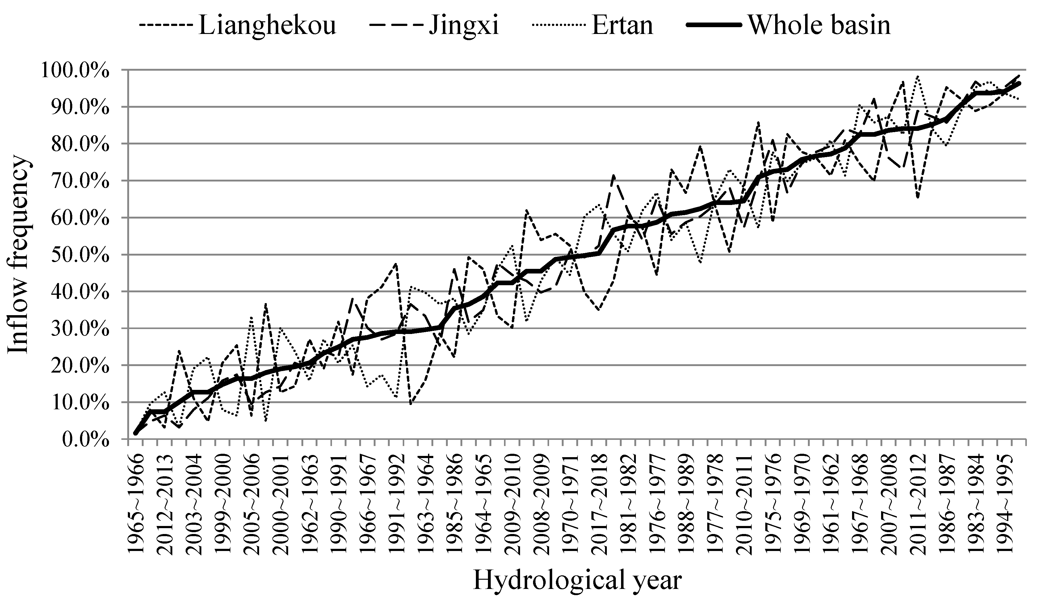
Using the aforementioned method of calculating the overall inflow frequency of the whole basin in Section 2.2, the overall inflow frequency of each year can be obtained, and they are shown in

Table 3. Inflow frequency of each station and the whole basin in each hydrological year.

Year	Liang-hekou	Jingxi	Ertan	Whole Basin	Year	Liang-hekou	Jingxi	Ertan	Whole Basin
1965–1966	1.6%	1.6%	1.6%	1.6%	2015–2016	39.7%	49.2%	60.3%	49.7%
1993–1994	7.9%	4.8%	9.5%	7.4%	2017–2018	34.9%	52.4%	63.5%	50.3%
2012–2013	3.2%	6.3%	12.7%	7.4%	1979–1980	42.9%	71.4%	55.6%	56.6%
1998–1999	23.8%	3.2%	3.2%	10.0%	1981–1982	60.3%	61.9%	50.8%	57.7%
2003–2004	11.1%	7.9%	19.0%	12.7%	2016–2017	57.1%	54.0%	61.9%	57.7%
2018–2019	4.8%	11.1%	22.2%	12.7%	1976–1977	44.4%	65.1%	66.7%	58.7%
1999–2000	20.6%	15.9%	7.9%	14.8%	1995–1996	73.0%	55.6%	54.0%	60.9%
1957–1958	25.4%	17.5%	6.3%	16.4%	1988–1989	66.7%	58.7%	58.7%	61.4%
2005–2006	6.3%	9.5%	33.3%	16.4%	1978–1979	79.4%	60.3%	47.6%	62.4%
1974–1975	36.5%	12.7%	4.8%	18.0%	1977–1978	63.5%	63.5%	65.1%	64.0%
2000–2001	12.7%	14.3%	30.2%	19.0%	2013–2014	50.8%	68.3%	73.0%	64.0%
1989–1990	14.3%	20.6%	23.8%	19.6%	2010–2011	68.3%	57.1%	68.3%	64.5%
1962–1963	27.0%	19.0%	15.9%	20.6%	1958–1959	85.7%	69.8%	57.1%	70.9%
1960–1961	19.0%	23.8%	27.0%	23.3%	1975–1976	58.7%	81.0%	77.8%	72.5%
1990–1991	31.7%	22.2%	20.6%	24.9%	1997–1998	82.5%	66.7%	69.8%	73.0%
1980–1981	17.5%	38.1%	25.4%	27.0%	1969–1970	77.8%	74.6%	74.6%	75.7%
1966–1967	38.1%	30.2%	14.3%	27.5%	1992–1993	76.2%	77.8%	76.2%	76.7%
1987–1988	41.3%	27.0%	17.5%	28.6%	1961–1962	71.4%	79.4%	81.0%	77.2%
1991–1992	47.6%	28.6%	11.1%	29.1%	1971–1972	81.0%	84.1%	71.4%	78.8%
2014–2015	9.5%	36.5%	41.3%	29.1%	1967–1968	74.6%	82.5%	90.5%	82.5%
1963–1964	15.9%	33.3%	39.7%	29.6%	1972–1973	69.8%	92.1%	85.7%	82.5%
2004–2005	28.6%	25.4%	36.5%	30.2%	2007–2008	87.3%	76.2%	87.3%	83.6%
1985–1986	22.2%	46.0%	38.1%	35.4%	2002–2003	96.8%	73.0%	82.5%	84.1%
2001–2002	49.2%	31.7%	28.6%	36.5%	2011–2012	65.1%	88.9%	98.4%	84.1%
1964–1965	46.0%	34.9%	34.9%	38.6%	1984–1985	84.1%	87.3%	84.1%	85.2%
1982–1983	33.3%	47.6%	46.0%	42.3%	1986–1987	95.2%	85.7%	79.4%	86.8%
2009–2010	30.2%	44.4%	52.4%	42.3%	1959–1960	92.1%	90.5%	88.9%	90.5%
1968–1969	61.9%	42.9%	31.7%	45.5%	1983–1984	88.9%	96.8%	95.2%	93.7%
2008–2009	54.0%	39.7%	42.9%	45.5%	2006–2007	90.5%	93.7%	96.8%	93.7%
1996–1997	55.6%	41.3%	49.2%	48.7%	1994–1995	93.7%	95.2%	93.7%	94.2%
1970–1971	52.4%	50.8%	44.4%	49.2%	1973–1974	98.4%	98.4%	92.1%	96.3%

and Figure 8 by ascending order.

In Figure 8, the abscissa is the year which corresponds to the ascending order of the overall inflow frequency of the river basin, so the year in abscissa is not in the order. From Figure 8, it can be seen that although the inflow frequencies of the three stations vary in the same year, they all fluctuate near the inflow frequency of the whole basin, and the overall trend of change is the same.

Because the typical runoff of dry years are needed in drawing ESOC, according to the results of Table 3, 10 dry years with the lowest frequency are selected, which are 2007–2008, 2002–2003, 2011–2012, 1984–1985, 1986–1987, 1959–1960, 1983–1984, 2006–2007, 1994–1995, 1973–1974.

3.2.2. Output Coefficients Optimization

In order to clearly express the steps of the output coefficients optimization mentioned in Section 2.3, we use a given output coefficient array to do the optimization. The results are as follows:

(1)

Provide the initial solution of output coefficients, such as (2.0, 1.8, 1.5, 1.2, 1, 1, 0.9, 0.8, 0.7, 0), draw the ESOC, and carry out the simulation. At this time, the corresponding average annual power generation is 1057.149 × 10⁸ kWh, and the guaranteed rate is 0.999.

(2)

After the first round of optimization, the optimal output coefficients are (2.2, 1.8, 1.2, 1, 1, 1, 1, 0.8, 0.7, 0, 0, 0), and the corresponding average annual power generation is 1060.0047 × 10⁸ kWh, the guaranteed rate is 0.991. Remove the repetition of 1 and 0, and change the number of curves to 8, then obtain the updated output coefficients, which are (2.2, 1.8, 1.2, 1, 1, 0.8, 0.7, 0).

(3)

After re-optimization, get the output coefficients (2.2, 1.8, 1, 1, 1, 1, 0.7, 0, 0, 0), and the average annual power generation is 1067.2245 × 10⁸ kWh, the guaranteed rate is 0.9858 at this moment. Remove the repetition of 1 and 0, and change the number of curves to 6, then, obtain the updated output coefficients, which is (2.2, 1.8, 1, 1, 0.7, 0).

(4)

Re-optimization again, the optimization results are (2.1, 1.8, 1, 1, 0, 0). At this time, the average annual power generation is 1067.482 × 10⁸ kWh, and the guaranteed rate is 0.9883. After removing the duplicate items, the results are (2.1, 1.8, 1, 1, 0).

(5)

Re-optimization again, the results are (2.1, 1.8, 1, 1, 0). At this time, the results of the adjacent two optimizations are no longer changed, so the final output coefficients, i.e., (2.1, 1.8, 1, 1, 0), are the optimal.

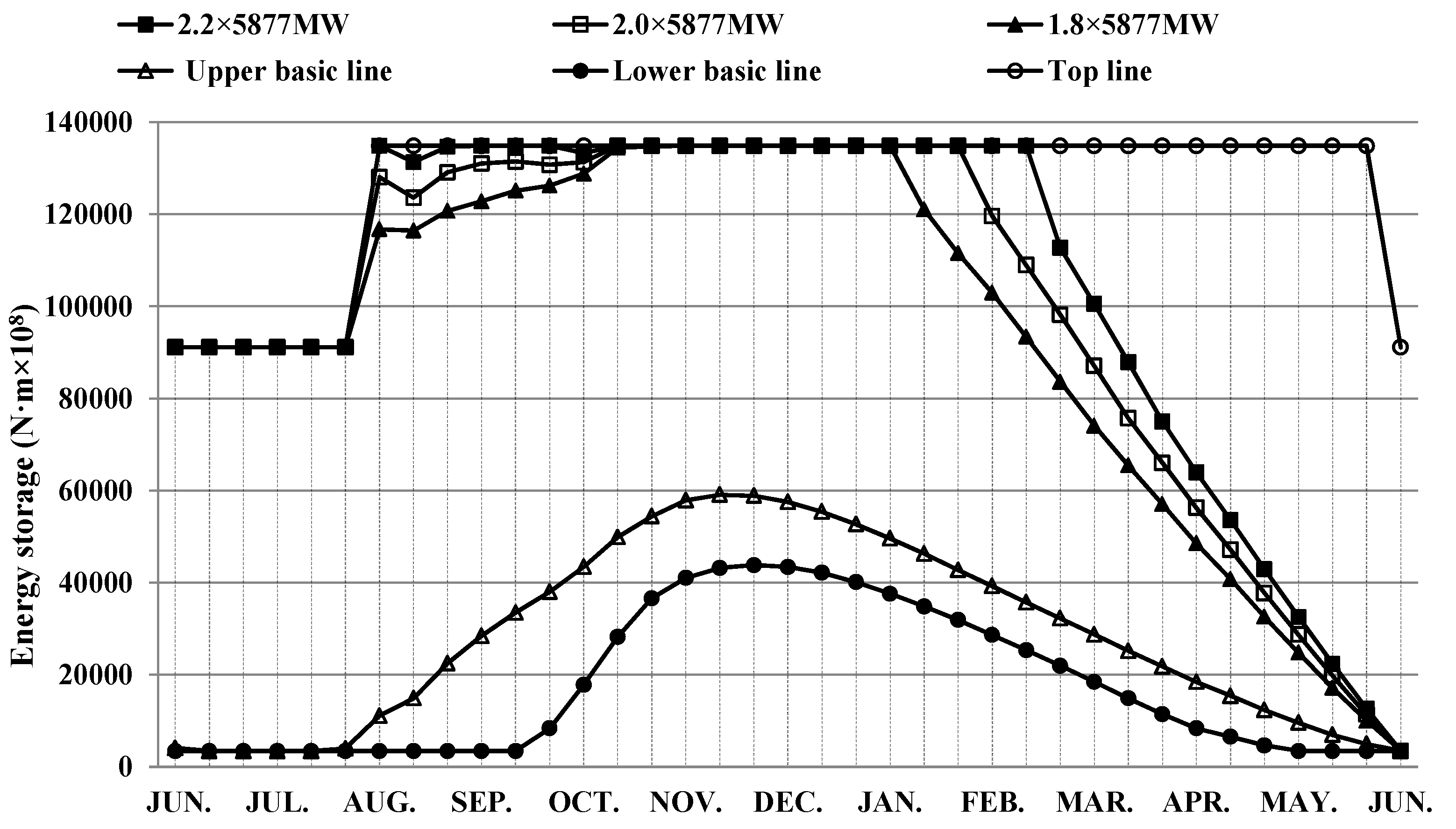
In the case study, we randomly generated 100 initial solutions with 5 times guaranteed output as the maximum output and 0.1 times guaranteed output as the output discrete interval, and optimized these initial solutions according to the above optimization steps. The final result of the optimal output coefficients is (2.2, 2, 1.8, 1, 1, 0). At this time, the corresponding average annual power generation is 1067.7624 × 10⁸ kWh and the guaranteed rate is 0.988. The corresponding ESOC is shown in Figure 9, in which 5877 MW is the cascade guaranteed output.

In order to show the advantages and effectiveness of the optimization method proposed in this paper, we used the output coefficients, i.e., (1.2, 1.1, 1, 1, 0.9, 0.8, 0), obtained in the literature by Jiang et al. (2016) to draw and simulate the ESOC of this basin. The obtained power generation is 979.4922 × 10⁸ kWh and the guaranteed rate is 0.999. It can be seen that although the guaranteed rate decreases to a certain extent after the optimization (from 0.999 to 0.988), the power generation has increased a lot, the absolute value has increased by 88.27 × 10⁸ kWh, and the relative value increased by 9%, which is very significant, and also shows the importance of optimizing the output coefficients of ESOC. For the guaranteed rate, in fact, both of them have reached more than 98.5%, even though there are some differences between them, it has no effect in practical application.

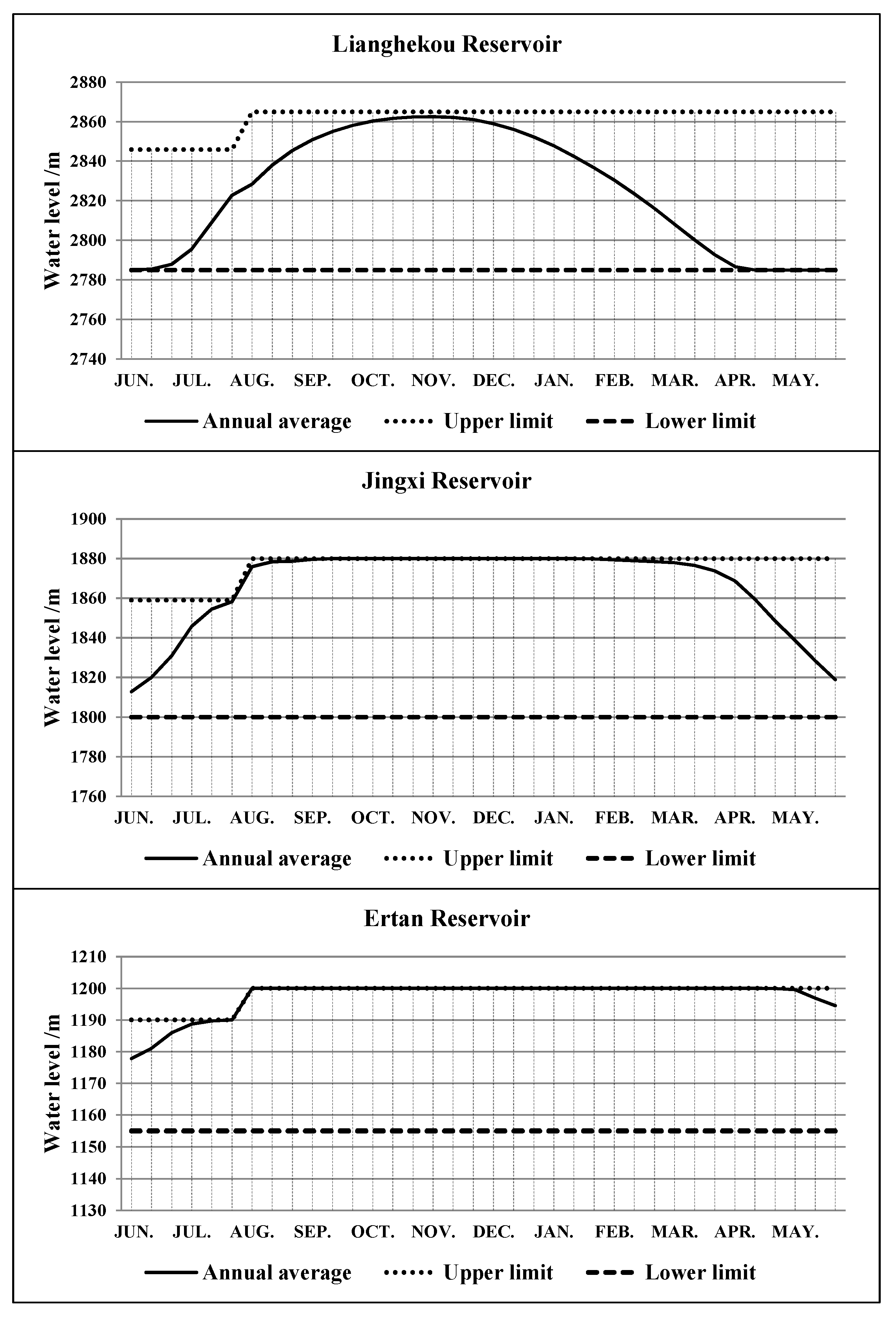
From Figure 9, it can be seen that the output zone of the operation chart is mainly divided into four zones, i.e., the guaranteed output zone, reduced output zone, 1.8 times guaranteed output zone, and 2.2 times guaranteed output zone. The scale of the 1.8 times guaranteed output zone is the largest. Through the simulation method described in Section 2.1, the multi-year average water level process of each reservoir can be obtained, and the results of the three reservoirs with regulating performance are shown in Figure 10.

From the water level variation of Figure 10, it can be seen that the water level processes of the three reservoirs are all within the upper and lower limits, and the water level variation of the Lianghekou reservoir is relatively gentle. Compared with the other two reservoirs (Jingxi and Ertan), the rising and falling processes of the water level of Lianghekou are lagging behind. The reason is that, in order to give full play to the head benefit of downstream reservoirs and increase the total cascade power generation, downstream reservoirs first store water in the wet season in order to increase the overall cascade water head as soon as possible. In the drawdown period, upstream reservoirs discharge the water before downstream reservoirs, so that the upstream reservoirs can make full use of the water head of downstream reservoirs. This result is also consistent with the control principle of discriminant coefficient method.

3.3.3. Optimization of Drawdown Level

In this basin, the Lianghekou is a multi-year regulating reservoir, and it is considered as an annual regulating reservoir in the above calculation. Therefore, it is necessary to determine an optimal annual average drawdown level for this reservoir. In order to determine this optimal drawdown level, by taking 5 meters as discrete step, a series of discretized water level values including 2785 m, 2790 m, 2795 m, 2800 m, 2805 m, 2810 m, 2815 m, 2820 m, 2825 m, 2830 m, 2835 m, 2840 m, and 2845 m are obtained on the basis of the original water level lower limit, i.e., 2785 m.

Respectively, taking the above discretized drawdown levels as the lower boundary of end-of-year operating water level in the ESOC model, the corresponding average annual power generation and guaranteed rate are obtained for each drawdown level, as shown in

Table 4. Results of power generation and guaranteed rate of Lianghekou under different drawdown levels.

Drawdown Level/m	2785	2790	2795	2800	2805	2810	2815	2820	2825	2830	2835	2840	2845
Power generation/108 kWh	103.8	104.7	105.7	106.6	107.6	108.5	109.2	109.9	110.7	111.4	112.0	112.3	112.1

and

Table 5. Results of cascade power generation and guaranteed rate under different drawdown levels.

Drawdown Level/m	Power Generation/108 kWh	Guaranteed Rate
2785	1067.8	98.80%
2790	1064.1	98.80%
2795	1060.5	98.60%
2800	1056.1	98.50%
2805	1051.6	98.30%
2810	1046.5	97.90%
2815	1041	97.10%
2820	1035.1	96.10%
2825	1028	94.20%
2830	1020	92.30%
2835	1012.6	89.90%
2840	1004.9	87.00%
2845	996.9	84.10%

. At this time, the output coefficient used in ESOC is (2.2, 2.0, 1.8, 1, 1, 1, 0).

Under the above drawdown levels, the variation of the average annual power generation of the Lianghekou reservoir itself is shown in Table 4. From Table 4, it can be seen that with the increase of drawdown level, the power generation of the Lianghekou reservoir increase gradually. Generally, with the rising of the drawdown level, the water head of the reservoir increases, but because of retaining a part of the water, the benefit of the water quantity will be reduced. However, generally speaking, the water head benefit is better than the water quantity benefit. Therefore, for the Lianghekou reservoir, the increase of drawdown level will increase the water head, and so that increases the power generation benefit.

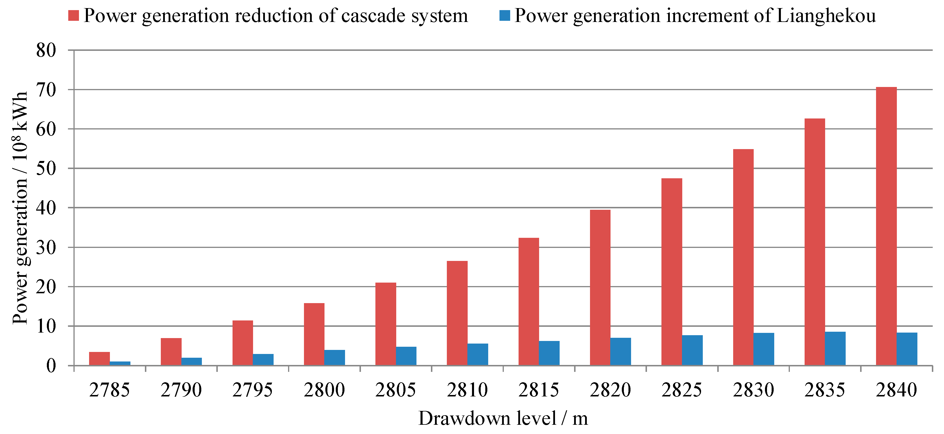
However, from table 5, it can be seen that, as for cascade system, with the rising of the drawdown level of the Lianghekou reservoir, the power generation of cascade system decreases gradually. The reason is that the sum of the water head of downstream reservoirs is very large. If the drawdown level of the Lianghekou reservoir rises and the reservoir retains a part of the water, the available water of the downstream reservoirs will be reduced, which makes the water head of the downstream reservoirs unable to produce benefits on this part of the water, so the total cascade power generation will be reduced.

Besides, it is found that, with increasing drawdown level, the reduction of cascade total power generation is greater than the power generation increment of the Lianghekou reservoir, as shown in Figure 11. Therefore, the optimal drawdown water level of the Lianghekou reservoir is 2785 m for the cascade system.

This result shows that, when the cascade system contains a multi-year regulating reservoir and it is located at the upstream of the basin (the sum of downstream water heads is relatively large at this point), the operation mode of the multi-year regulating reservoir under joint operation is quite different from the single reservoir operation. When a multi-year regulating reservoir is operated alone, considering the head benefit of the reservoir itself and the water consumption in subsequent years, its water level generally does not drawdown to the dead water level, and there is an optimum drawdown level. However, when a multi-year regulating reservoir is jointly operated with other reservoirs, considering the water head benefit of downstream reservoirs, the multi-year regulating reservoir will not retain water, but will fall to the dead water level at the end of the year.

4. Summary and Conclusions

Taking the cascade system of seven reservoirs in the Yalong River basin as an example, this paper studied the optimal selection of typical runoff of dry years considering the inflow frequency inconsistency of the basin, the optimization of the output coefficients of ESOC, and the optimization of ESOC in which the multi-year regulating reservoir is included, and the following conclusions can be summarized.

(1)

The proposed selection method of typical dry years based on the minimum square sum of frequency difference can effectively consider the inflow frequency inconsistency of upstream and downstream and make the typical runoff processes representing the whole basin more reasonable. In the case study, we selected 10 dry years with the lowest frequencies by this method, and the ESOC is drawn based on this.

(2)

The optimization method of output coefficients and the method of generating an initial solution proposed in this paper can quickly and accurately find out the best output coefficients, and effectively solve the influence of output coefficients on the results of ESOC. In the case study, under the optimal output coefficients, the annual average power generation of the seven reservoirs in Yalong River can reach 1067.76 × 10⁸ kWh, and compared with previous research results the total power generation of cascade system increased by 9%.

(3)

Aiming at the end-of-year drawdown level problem of multi-year regulating reservoirs, through the case study, it is found that when a multi-year regulating reservoir participates in the joint operation of cascade system and the sum of downstream reservoirs is large, the optimum of end-of-year drawdown level is the lower limit of the allowable operating water level range, and this conclusion is different from that of a multi-year regulating reservoir operated alone.

References

- Yüksel, I. Hydropower for sustainable water and energy development. Renew. Sustain. Energy Rev. 2010, 14, 462–469. [Google Scholar] [CrossRef]
- Platero, C.A.; Sanchez, J.A.; Nicolet, C.; Allenbach, P. Hydropower Plants Frequency Regulation Depending on Upper Reservoir Water Level. Energies 2019, 12, 1637. [Google Scholar] [CrossRef]
- Lakshminarasimman, L.; Subramanian, S. A modified hybrid differential evolution for short-term scheduling of hydrothermal power systems with cascaded reservoirs. Energy Convers. Manag. 2008, 49, 2513–2521. [Google Scholar] [CrossRef]
- Yeh, W.W.G. Reservoir management and operations models: A state-of-the-art review. Water Resour. Res. 1985, 21, 1797–1818. [Google Scholar] [CrossRef]
- Ji, C.; Jiang, Z.; Sun, P.; Zhang, Y.; Wang, L. Research and Application of Multidimensional Dynamic Programming in Cascade Reservoirs Based on Multilayer Nested Structure. J. Water Resour. Plan. Manag. 2015, 141, 04014090. [Google Scholar] [CrossRef]
- Connaughton, J.; King, N.; Dong, L.; Ji, P.; Lund, J. Comparing simple flood reservoir operation rules. Water 2014, 6, 2717–2731. [Google Scholar] [CrossRef]
- Adeloye, A.J.; Soundharajan, B.S.; Ojha, C.S.P.; Remesan, R. Effect of hedging-integrated rule curves on the performance of the pong reservoir (India) during scenario-neutral climate change perturbations. Water Resour. Manag. 2016, 30, 445–470. [Google Scholar] [CrossRef]
- Hojjati, A.; Monadi, M.; Faridhosseini, A.; Mohammadi, M. Application and comparison of NSGA-II and MOPSO in multi-objectives optimization of water resources systems. J. Hydrol. Hydromech. 2018, 66, 323–329. [Google Scholar] [CrossRef]
- Ming, B.; Liu, P.; Guo, S.; Cheng, L.; Zhou, Y.; Gao, S.; Li, H. Robust Hydroelectric Unit Commitment Considering Integration of Large-scale Photovoltaic Power: A Case Study in China. Appl. Energy 2018, 228, 1341–1352. [Google Scholar] [CrossRef]
- Yuan, X.; Wang, P.; Yuan, Y. A new quantum inspired chaotic artificial bee colony algorithm for optimal power flow problem. Energy Convers. Manag. 2015, 100, 1–9. [Google Scholar] [CrossRef]
- Jabr, R.A.; Coonick, A.H.; Cory, B.J. A homogeneous linear programming algorithm for the security constrained economic dispatch problem. IEEE Trans. Power Syst. 2000, 15, 930–936. [Google Scholar] [CrossRef]
- Vincenzo, M.; Gianfranco, R.; Francesco, A.T. Application of dynamic programming to the optimal management of a hybrid power plant with wind turbines, photovoltaic panels and compressed air energy storage. Appl. Energy 2012, 97, 849–859. [Google Scholar]
- Jiang, Z.; Qiao, Y.; Chen, Y.; Ji, C. A New Reservoir Operation Chart Drawing Method Based on Dynamic Programming. Energies 2018, 11, 3355. [Google Scholar] [CrossRef]
- Feng, Z.; Niu, W.; Cheng, C. Optimizing electrical power production of hydropower system by uniform progressive optimality algorithm based on two-stage search mechanism and uniform design. J. Clean. Prod. 2018, 190, 432–442. [Google Scholar] [CrossRef]
- Baskar, S.; Subbaraj, P.; Rao, M.V.C. Hybrid real coded genetic algorithm solution to economic dispatch problem. Comput. Electr. Eng. 2003, 29, 407–419. [Google Scholar] [CrossRef]
- Xu, B.; Zhong, P.; Wan, X.; Zhang, W.; Chen, X. Dynamic Feasible Region Genetic Algorithm for Optimal Operation of a Multi-Reservoir System. Energies 2012, 5, 2894–2910. [Google Scholar] [CrossRef] [Green Version]
- Ahmadi, M.; Haddad, O.B.; Loáiciga, H.A. Adaptive Reservoir Operation Rules Under Climatic Change. Water Resour. Manag. 2014, 29, 1247–1266. [Google Scholar] [CrossRef]
- Zhang, R.; Zhou, J.; Zhang, H.; Liao, X.; Wang, X. Optimal Operation of Large-Scale Cascaded Hydropower Systems in the Upper Reaches of the Yangtze River, China. J. Water Resour. Plan. Manag. 2014, 140, 480–495. [Google Scholar] [CrossRef]
- Yu, X.; Sun, H.; Wang, H.; Liu, Z.; Zhao, J.; Zhou, T.; Qin, H. Multi-Objective Sustainable Operation of the Three Gorges Cascaded Hydropower System Using Multi-Swarm Comprehensive Learning Particle Swarm Optimization. Energies 2016, 9, 438. [Google Scholar] [CrossRef]
- Nabinejad, S.; Jamshid Mousavi, S.; Kim, J.H. Sustainable Basin-Scale Water Allocation with Hydrologic State-Dependent Multi-Reservoir Operation Rules. Water Resour. Manag. 2017, 31, 3507–3526. [Google Scholar] [CrossRef]
- Dehghani, M.; Riahi-Madvar, H.; Hooshyaripor, F.; Mosavi, A.; Shamshirband, S.; Zavadskas, E.K.; Chau, K. Prediction of Hydropower Generation Using Grey Wolf Optimization Adaptive Neuro-Fuzzy Inference System. Energies 2019, 12, 289. [Google Scholar] [CrossRef]
- Ding, Z.; Fang, G.; Wen, X.; Tan, Q.; Huang, X.; Lei, X.; Tian, Y.; Quan, J. A novel operation chart for cascade hydropower system to alleviate ecological degradation in hydrological extremes. Ecol. Model. 2018, 384, 10–22. [Google Scholar] [CrossRef]
- Tayebiyan, A.; Mohammad, T.A.; Al-Ansari, N.; Malakootian, M. Comparison of optimal hedging policies for hydropower reservoir system operation. Water 2019, 11, 121. [Google Scholar] [CrossRef]
- Liu, P.; Guo, S.; Xu, X.; Chen, J. Derivation of Aggregation-Based Joint Operating Rule Curves for Cascade Hydropower Reservoirs. Water Resour. Manag. 2011, 25, 3177–3200. [Google Scholar] [CrossRef]
- Ostadrahimi, L.; Mariño, M.A.; Afshar, A. Multi-reservoir Operation Rules: Multi-swarm PSO-based Optimization Approach. Water Resour. Manag. 2012, 26, 407–427. [Google Scholar] [CrossRef]
- Taghian, M.; Rosbjerg, D.; Haghighi, A.; Madsen, H. Optimization of conventional rule curves coupled with hedging rules for reservoir operation. J. Water Resour. Plan. Manag. 2014, 140, 693–698. [Google Scholar] [CrossRef]
- Bolouri-Yazdeli, Y.; Bozorg Haddad, O.; Fallah-Mehdipour, E.; Mariño, M.A. Evaluation of real-time operation rules in reservoir systems operation. Water Resour. Manag. 2014, 28, 715–729. [Google Scholar] [CrossRef]
- Li, L.; Liu, P.; Rheinheimer, D.; Deng, C.; Zhou, Y. Identifying Explicit Formulation of Operating Rules for Multi-Reservoir Systems Using Genetic Programming. Water Resour. Manag. 2014, 28, 1545–1565. [Google Scholar] [CrossRef]
- Aboutalebi, M.; Bozorg Haddad, O.; Loáiciga, H.A. Optimal monthly reservoir operation rules for hydropower generation derived with SVRNSGAII. J. Water Resour. Plan. Manag. 2015, 141, 04015029. [Google Scholar] [CrossRef]
- Jiang, Z.; Li, A.; Ji, C.; Qin, H.; Yu, S.; Li, Y. Research and application of key technologies in drawing energy storage operation chart by discriminant coefficient method. Energy 2016, 114, 774–786. [Google Scholar] [CrossRef]
- Ashrafi, S.M.; Dariane, A.B. Coupled Operating Rules for Optimal Operation of Multi-Reservoir Systems. Water Resour. Manag. 2017, 31, 4505–4520. [Google Scholar] [CrossRef]
- Jiang, Z.; Ji, C.; Qin, H.; Feng, Z. Multi-stage Progressive Optimality Algorithm and its application in energy storage operation chart optimization of cascade reservoirs. Energy 2018, 148, 309–323. [Google Scholar] [CrossRef]
- Jiang, Z.; Qin, H.; Hu, D.; Ji, C.; Zhou, J. Effect Analysis of Operation Stage Difference on Energy Storage Operation Chart of Cascade Reservoirs. Water Resour. Manag. 2019, 33, 1349–1365. [Google Scholar] [CrossRef]
- Jiang, Z.; Liu, P.; Ji, C.; Zhang, H.; Chen, Y. Ecological Flow Considered Multi-Objective Storage Energy Operation Chart Optimization of Large-Scale Mixed Reservoirs. J. Hydrol. 2019, 577, 123949. [Google Scholar] [CrossRef]
- Wang, L.; Sun, P.; Jiang, Z.; Wang, B.; Zhang, Y. Study on cascade energy storage operation chart optimization of Li Xianjiang basin Based on Progressive Optimal Algorithm. Adv. Mater. Res. 2015, 1073–1076, 1641–1650. [Google Scholar] [CrossRef]
- Zhao, T.; Cai, X.; Lei, X.; Wang, H. Improved Dynamic Programming for Reservoir Operation Optimization with a Concave Objective Function. J. Water Resour. Plan. Manag. 2012, 138, 590–596. [Google Scholar] [CrossRef]
- Feng, Z.; Niu, W.; Cheng, C.; Wu, X. Optimization of large-scale hydropower system peak operation with hybrid dynamic programming and domain knowledge. J. Clean. Prod. 2018, 171, 390–402. [Google Scholar] [CrossRef]
Figure 1.
Inverse calculation process of drawing basic operation curves.
Figure 2.
Inverse calculation process of drawing the increased and reduced output curves.
Figure 3.
Sketch Map of operation curves optimization by Progressive Optimality Algorithm (POA).
Figure 4.
Possible space for initial solution of output coefficients of Energy Storage Operation Chart (ESOC).
Figure 5.
Optimization process of output variation coefficient.
Figure 6.
Optimization flowchart of drawdown level of a multi-year regulating reservoir.
Figure 7.
Geographic locations of Yalong River cascade reservoirs.
Figure 8.
Inflow frequency (ascending order) of the whole basin in each hydrological year.
Figure 9.
Optimal energy storage operation chart.
Figure 10.
Multi-year average water level process of the three regulating reservoirs.
Figure 11.
Comparison of reduction of cascade total power generation and increment of Lianghekou power generation.