Article

Evaluation of TsHARP Utility for Thermal Sharpening of Sentinel-3 Satellite Images Using Sentinel-2 Visual Imagery

1
The Blaustein Institutes for Desert Research, Ben-Gurion University of the Negev, Sede Boqer Campus, Midreshet, Ben-Gurion 84990, Israel
2
Institute of Agricultural Engineering, Agricultural Research Organization (ARO), Volcani Center, Midreshet Ben-Gurion 84990, Israel
3
Hydrology and Remote Sensing Laboratory, Agricultural Research Services, US Department of Agriculture, Beltsville, MD 20705, USA
*
Author to whom correspondence should be addressed.
Remote Sens. 2019, 11(19), 2304; https://doi.org/10.3390/rs11192304
Submission received: 19 August 2019 / Revised: 18 September 2019 / Accepted: 24 September 2019 / Published: 3 October 2019

Abstract

:
A spatially distributed land surface temperature is important for many studies. The recent launch of the Sentinel satellite programs paves the way for an abundance of opportunities for both large area and long-term investigations. However, the spatial resolution of Sentinel-3 thermal images is not suitable for monitoring small fragmented fields. Thermal sharpening is one of the primary methods used to obtain thermal images at finer spatial resolution at a daily revisit time. In the current study, the utility of the TsHARP method to sharpen the low resolution of Sentinel-3 thermal data was examined using Sentinel-2 visible-near infrared imagery. Compared to Landsat 8 fine thermal images, the sharpening resulted in mean absolute errors of ~1 °C, with errors increasing as the difference between the native and the target resolutions increases. Part of the error is attributed to the discrepancy between the thermal images acquired by the two platforms. Further research is due to test additional sites and conditions, and potentially additional sharpening methods, applied to the Sentinel platforms.

Graphical Abstract

1. Introduction

The land surface temperature (LST) at both high spatial and temporal resolutions is a key variable in many environmental studies, including vegetation monitoring, moisture estimation [1,2], drought assessment, evapotranspiration mapping [3,4,5], land-cover classification [6], and surface energy balance quantification [7]. However, until recently, satellite-derived LST has been provided at either a high temporal resolution (1 day) but low spatial resolution (1 km), e.g., National Oceanic and Atmospheric Administration–Advanced Very High Resolution Radiometer (NOAA-AVHRR) and Moderate Resolution Imaging Spectrometer (MODIS)-Terra/Aqua, or at a higher spatial resolution (60–120 m) but a low revisit time of 16 days, e.g., Landsat Thematic Mapper (TM) - Enhanced Thematic Mapper Plus (ETM+)/ Operational Land Imager (OLI).
To bridge this gap, attempts have been made to downscale frequently acquired low spatial resolution thermal images in order to assess LST at a high spatial resolution, and further use the data for the above-mentioned applications. The downscaling methods can be roughly classified into two categories: temperature unmixing and thermal sharpening [8,9,10,11]. Temperature unmixing is based on obtaining a coarse resolution temperature for different land-cover types and applying a split-window algorithm to retrieve the fine resolution results [12,13,14]. Thermal sharpening methods are based on a correlation between thermal images and auxiliary data (e.g., Normalized Difference Vegetation Index (NDVI), emissivity, albedo, digital elevation model, and normalized multi-band drought index (NMDI)). A variety of sharpening methods have been proposed, among which are DisTrad [7], STARFM [15], TsHARP [16,17], Artificial Neural Networks [18], the Data Mining Approach (DMS) [19], and NL-DisTrad [20].
DisTrad utilizes the quadratic relationship between NDVI and LST [7]. Bindhu et al. [20] applied a non-linear method, based on the DisTrad algorithm, to disaggregate the land surface temperature of MODIS with a 960-m spatial resolution to Landsat ETM+ at 60-m resolution over India. Agam et al. [17] improved the DisTrad algorithm by correlating the LST data with fractional vegetation cover (fc) instead of NDVI. The algorithm, termed TsHARP, was developed and tested over homogeneous fields in central Iowa, USA, and was proposed to disaggregate LST values over agricultural fields for monitoring irrigation processes and evaluating evapotranspiration [16,17,20,21]. It was demonstrated that sharpening thermal data at 960 m to 250 m, mimicking the sharpening of MODIS thermal to visible-near infrared (VNIR) data, yields root-mean-square-errors (RMSE) of between 0.67 and 1.35 °C. Sharpening thermal Landsat data from 120 and 60 m to a VNIR resolution of 20 m resulted in an RMSE of 1.8–2.4 °C. TsHARP was also tested over different land cover types, moisture conditions, and vegetation types [22,23,24,25]. Bisquert et al. [22] sharpened MODIS images with TsHARP with mean errors of 1.9 °C between disaggregated and reference Landsat thermal images at a 120-m spatial resolution. TsHARP’s utility was able to disaggregate MODIS temperature from 1000 m to 90 m with an error of 2.7 °C [26].
Among all the sharpening methods, TsHARP is the most widely used due to its simplicity and effectiveness. Bisquert et al. [27] examined three downscaling methods with MODIS and Landsat images in the heterogeneous vegetated area of central Spain and reported that TsHARP outperformed the others. Improving TsHARP was proposed by using a local modification of utility [24] and by combining it with spatial interpolation [23]. Jeganathan et al. [24] tested five different versions of TsHARP over a heterogeneous agricultural landscape in India. The methods were applied to aggregated data from the Advanced Spaceborne Thermal Emission and Reflection Radiometer (ASTER) and used for MODIS thermal maps. The local aggregation model yielded higher accuracy. Chen et al. [23] combined TsHARP with thin plate spline interpolation, which improved the sharpening accuracy by about 10% for grasslands and 5% for rural areas and croplands. Despite these encouraging results, the fact that TsHARP is based on the LST–NDVI relationship makes it inapplicable when this relationship is weak or reversed [28,29].
The recent initiation of the Copernicus Earth observation program of the European Commission (EC) and the European Space Agency (ESA), and the launch of the Sentinel constellation of satellites provides new opportunities to further examine the potential of TsHARP. Sentinel-2A and Sentinel-2B were launched on 23 June, 2015 and 7 March, 2017, respectively. The MultiSpectral Instrument (MSI) onboard these satellites has VNIR bands at around 6.65 and 8.35 µm, which enables the calculation of different vegetation indices for vegetation characterization at a 10-m resolution. This constellation has a revisit time of five days. Sentinel-3A and Sentinel-3B were launched on 16 February, 2016 and 25 April, 2018, respectively. The Sea and Land Surface Temperature Radiometer (SLSTR) on board these satellites has two thermal bands, at 10.8 and 12 µm, which acquires LST at a ~1-km resolution at nadir. The Sentinel-3 constellation has a revisit time of less than two days [30]. The remarkable advantages of sharpening the Sentinel-3 LST to the VNIR resolution of the Sentinel-2 are that the Sentinel satellites are synchronized in overpass time and ground coverage, and the images are in the same projection and processing chain. Moreover, archived data are available free-of-charge by the Copernicus Open Access Hub through several platforms (https://scihub.copernicus.eu). Lastly, the planned life cycle of the satellites is 15–20 years [31]. A first attempt to sharpen Sentinel-3 LST using Sentinel-2 NVIR data has recently been published [32]. A methodology to derive land-surface energy fluxes using the DMS approach was tested in agricultural and forest sites located in temperate zones. The results of the study indicated an improvement in derived energy fluxes from sharpened LST in comparison with low-resolution fluxes. However, the fluxes were still less accurate than those derived from high-resolution LST. The overarching goal of the current project was to examine the utility of TsHARP to sharpen the Sentinel-3 thermal data using Sentinel-2 VNIR imagery.

2. Materials and Methods
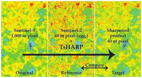
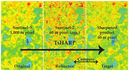
2.1. TsHARP Method

The TsHARP algorithm is based on the linear correlation between LST and fractional vegetation cover (fc). A detailed description of the TsHARP procedure is given in Agam et al. [17]. An empirical linear regression model is fitted to the LST and fc data at the native coarse resolution of the LST image after aggregating the fine (target) resolution fc image to match the coarse resolution of the LST image (LSTcoarse and fc coarse, Equation (1)).
LST coarse = a + bf c _ coarse  
with fc computed as follows (Equation (2)).
f c = 1   ( NDVI max   NDVI i   NDVI max     NDVI min   ) 0.625
where NDVIi is the index value in a specific pixel while NDVImax and NDVImin are the maximum and minimum values from the scene, respectively [33].
Assuming that the correlation between LST and fc is scale-independent, the resulting regression coefficients (a and b) obtained at the low resolution are applied to the fine spatial resolution vegetation index together with the fine resolution fc data (fc fine) to predict the regression-based LST at the target fine resolution (LSTfine, Equation (3)). Lastly, the residual error (i.e., the difference between the native, LSTnative, and the estimated, LSTcoarse, temperatures) for the corresponding coarse resolution pixel is added to the predicted temperature to increase the prediction accuracy (Equation (4)).
LST fine = a +   bf c   fine  
LST downscale =   LST fine + ( LST initial     LST coarse )

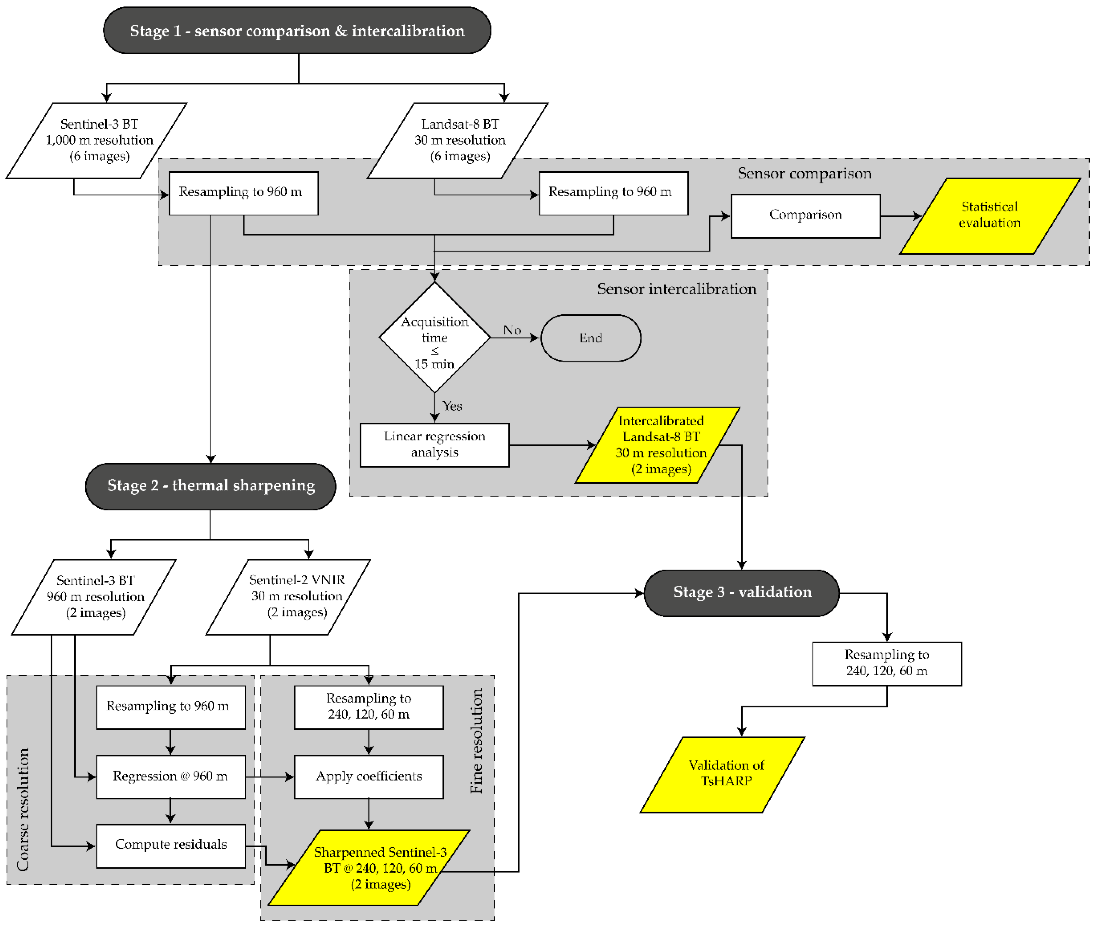
2.2. Methodological Workflow
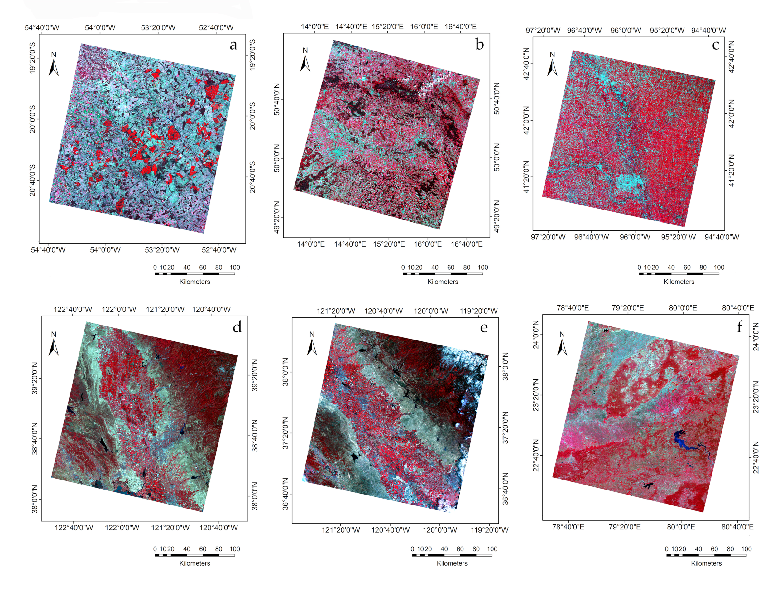
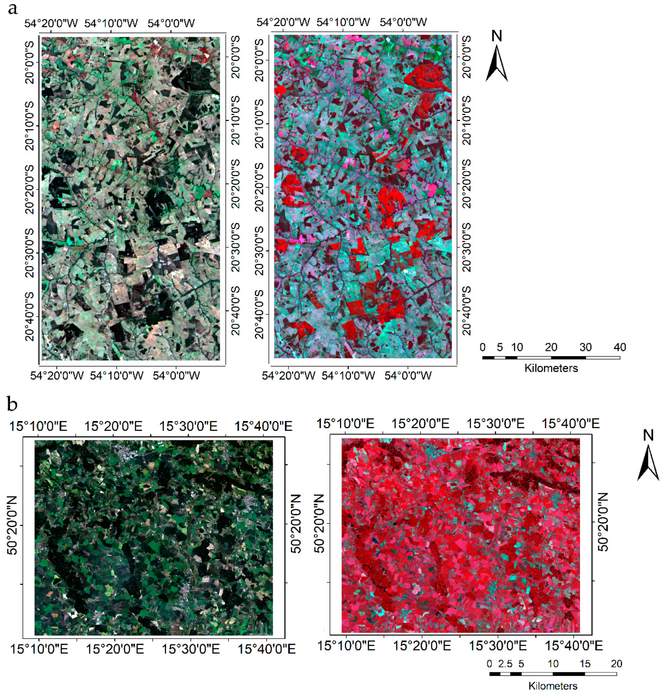
Testing the accuracy of TsHARP for sharpening Sentinel-3 thermal images using Sentinel-2 VNIR images was assessed by comparing the sharpened thermal images to Landsat-8 thermal images that were acquired at a fine resolution. This was applied in three stages (Figure 1).
Stage 1–sensor comparison and inter-calibration–before using Landsat-8 to validate the sharpening product, the comparability between the Sentinel-3 and the Landsat-8 thermal images had to be evaluated. To this end, six pairs of Sentinel-3 vs. Landsat-8 thermal images, acquired within a maximum of a 15-minute time difference, were compared. To minimize potential additional sources of error due to different atmospheric corrections between the two sensors [34], the comparison, as well as the sharpening, was applied on top-of-atmosphere brightness temperature (BT) images, which has been previously done (e.g., [19,25,35]). The six BT image-pairs were compared at the coarse resolution of 960 m (see more in Section 2.4 hereafter). For the following analyses, two of the six pairs of images, for which a coinciding same-day Sentinel-2 overpass was available (Table 1), were chosen. For these two pairs, the linear regression coefficients resulting from regressing the Sentinel-3 BT values against the Landsat-8 BT values were used to calibrate the images. The calibrated Landsat-8 BT images were used in Stage 3 for validation (see below).
Stages 2 and 3 were, as mentioned, based on an analysis of two sites only, for which images from all three satellites were available. In Stage 2–thermal sharpening–the TsHARP algorithm was applied over the two sites, and, in Stage 3–validation–the accuracy of TsHARP was evaluated by a visual and statistical comparison.

2.3. Study Sites

Six areas representing different climatic conditions and land-cover types were selected (Table 1 and Figure 2).
- Site 1–Campo Grande, Brazil
A relatively homogeneous landscape characterized by extensive savanna formations crossed by forests and stream valleys. The altitude of the site ranges from 298 to 764 m. The area includes irrigated and rainfed wheat, corn, barley, rice, and soybeans fields, orchards, natural sand banks, savannahs, open pastures, and bushes. The climate is classified as subtropical and tropical with an annual mean temperature of 24 °C and annual mean precipitation of 1471 mm [36].
- Site 2–Podebrady, Czech Republic
Lying in a temperate climate zone with annual precipitation of about 660 mm, this site is characterized by mild and humid summers with an average annual temperature of 8.8 °C. The altitude varies from 146 to 1,385 m. This site contains mixed evergreen and broadleaves forests, urban areas, croplands, pastures, orchards, wetlands, and water bodies. Most agricultural fields are planted with winter wheat, barley, sugar beet, rapeseed, and maize.
- Site 3–Iowa-Nebraska border near Omaha, Nebraska, USA
A relatively flat plain with an average altitude of 310 m above mean sea level (a.m.s.l) dominated by croplands, mainly corn and soybean fields (93%), with a minority of sorghum, oats, and wheat. Small areas of forest, grassland, riparian vegetation, and urban regions occur within the scene. The area is characterized by a humid continental climate, with an annual precipitation rate of 700 mm and an annual temperature of 10.5 °C.
- Sites 4 and 5 are located near Sacramento, California, USA
These areas are predominantly agricultural landscapes with mainly irrigated rice fields. Other common crops are grapes, citrus, almonds, and lettuce. A small fraction of the area comprises grasslands, hay fields, and cattle ranches. The climate in the region is Mediterranean with average annual high and low temperatures of 24.2 °C and 9.2 °C, respectively, and average precipitation of 485 mm that falls predominantly during the winter season (November–March). The altitude reaches a maximum of about 2,230 m. Site five has a 15-minute gap between Landsat 8 and Sentinel-3 imagery, while images were extracted at the same time at Site 4.
- Site 6–Madhya Pradesh District, India
This is a fertile land region with the main crop production of wheat, pulses, rice, oilseeds, sorghum, soybean, and sugarcane. The average field size is 0.5 x 0.8 km, which is the smallest among all sites, with the most diverse land cover. Other land covers found in the scene are ponds, grasslands, savannas, hills, urban areas, and bushes. The climate is humid subtropical, with hot and dry summers and cold and wet winters. The annual rainfall of the region is 1218 mm with an average annual high and low temperatures of 33 °C and 18 °C, respectively. The altitude of the region varies from 312–970 m.
All scenes correspond to entire tiles of Landsat 8. The outlines in Panels b and e in Figure 2 delineate the analyzed areas for Site 2 and Site 5 since Sentinel-3 did not cover the whole Landsat scene (Site 2) and to avoid clouds (Sites 5).
Sites 1 and 2, for which Sentinel-3, Sentinel-2, and Landsat 8 overlapped (Figure 3), were used to perform the inter-calibration of NDVI maps (Stage 1, Figure 1), as well as to apply TsHARP (Stage 2, Figure 1) and to validate the sharpening results (Stage 3, Figure 1).

2.4. Data

Thermal images from Landsat 8 OLI and Sentinel-3 Sea and Land Surface Temperature Radiometer (SLSTR) were collected in June–October 2017. Landsat 8 OLI images containing VNIR and shortwave infrared (SWIR) with 30-m spatial resolutions were downloaded from the official USGS website (http://earthexplorer.gov.by). Landsat 8’s native thermal resolution is 100 m, but only the 30-m images disaggregated by the Landsat Science Team were available publicly. The Sentinel-3 SLSTR products were provided by the Scientific Sentinel Hub (http://scihub.copernicus.eu/). They consist of two thermal bands at a 1,000-m spatial resolution in addition to the VNIR bands at a 500-m spatial resolution.
The Sentinel-2A data are composed of 13 spectral bands in the VNIR region resolutions ranging from 10 to 60 m. The Sentinel-2 tile has a small fixed size of 100 x 100 km, so the selection of satellite images was limited to the overlapping areas of the Landsat and Sentinel overpasses.

2.5. Data Processing

Landsat 8 images were calibrated to top-of-atmosphere reflectance and brightness temperature using the Landsat Ecosystem Disturbance Adaptive Processing System [37]. Then, the reflectance maps were atmospherically and geometrically corrected using the ATCOR module included in the ERDAS IMAGINE software [38]. The atmospherically corrected red and near-infrared bands were used to calculate NDVI. Water and artificial pixels were masked out using supervised classification since they do not conform to the NDVI–BT relationship. Landsat 8 BT images were aggregated to 960 m, which is the closest multiple of 30 m to the 1,000-m resolution of the Sentinel-3 BT images. These images were used to sharpen Landsat-to-Landsat to eliminate errors stemming from the differences between sensors. In addition, Landsat 8 BT images were aggregated to 60, 120, and 240 m. All three were used for validating the sharpening into these three resolutions to test the accuracy dependency on the target resolution. Aggregation was conducted after converting BT to radiance, according to the Stefan-Boltzmann Law, and converted it back to BT at the coarse resolution. Lastly, Sentinel-3 BT images were resampled to 960 m, to match the aggregated resolution of Landsat 8. The Sentinel-3 BT images were re-projected and geo-registered to the same reference system of the UTM Zone to match Landsat 8 thermal imagery. The Sentinel-2A dataset was atmospherically corrected with sen2cor software [39]. Band 8a (near-infrared, 20-m pixel size) and band 4 (Red, 10-m pixel size) were used to calculate NDVI.

2.6. TsHARP Performance Assessment

To evaluate the sharpening accuracy of Sentinel-3 BT images (BTsentinel3) to a finer resolution based on VNIR data acquired by Sentinel-2, fine-resolution BT images acquired by Landsat 8 (BTlandsat) were used. To evaluate the uncertainty caused by comparing results from different sensors, a two-step analysis was performed. First, BTlandsat was aggregated to the coarse resolution of BTsentinel3 on which the sharpening algorithms were applied. The sharpened images were then compared to the original BTlandsat. After that, BTsentinel3 were sharpened and compared to BTlandsat. This allowed the isolation of errors that were solely due to differences between the two sensors, which are irrespective of the sharpening procedure.
The level of agreement between the reference and the sharpened temperatures was estimated by root-mean-square error (RMSE), mean absolute error (MAE), bias, the coefficient of determination (R2), and the normalized root-mean-square error (nRMSE); Equations (5)–(9), respectively [40].
RMSE =   n 1 i = 1 n ( T sharp T ref   ) 2 1 / 2
MAE =   n 1 i = 1 n ( T sharp T ref   )
R 2 = 1   ( T sharp     T ref ) 2 ( T sharp     T ref _ mean ) 2
bias =   i = 1 n ( T sharp T ref   ) n
nRMSE =   RMSE T max   T min
where Tsharp is the sharpened temperature, Tref and Tref_mean are the reference temperature and the average of the reference temperature in the entire image, respectively, and Tmax and Tmin are the maximum and minimum temperature values, respectively.

3. Results and Discussion

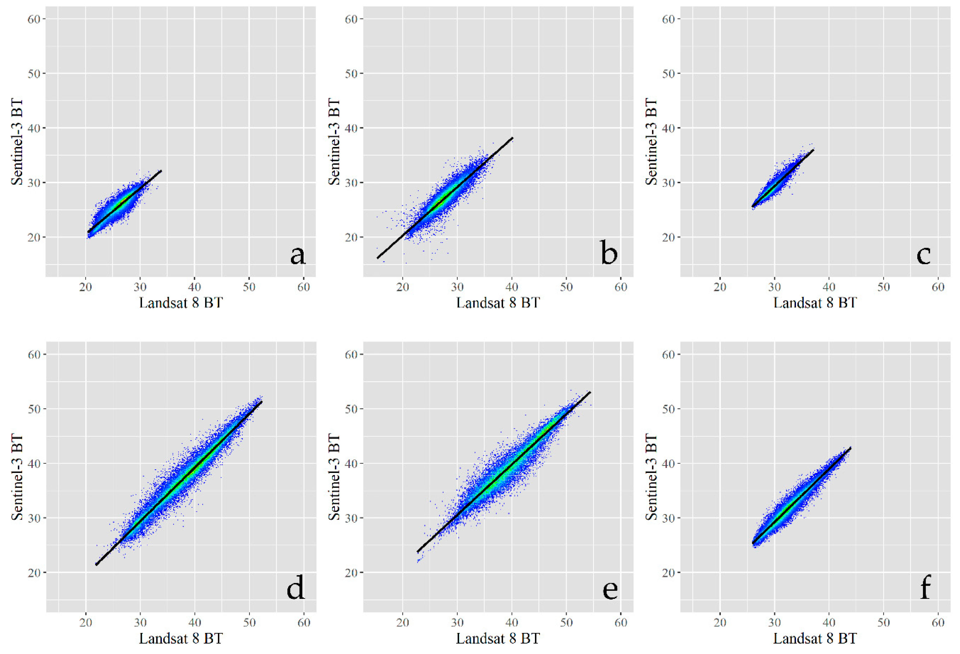
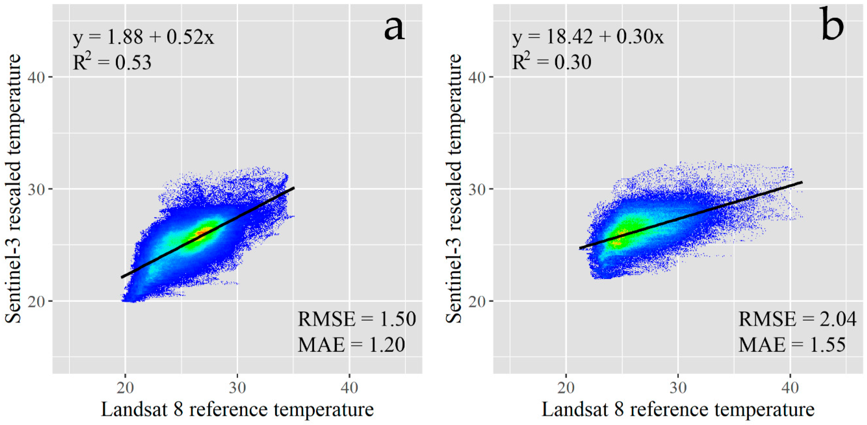
3.1. Sensor Intercalibration of Brightness Temperature

The surface temperature rapidly changes, especially during the mid-morning. The typical overpass time of many satellites including Landsat and Sentinel. A comparison between sensors is, thus, challenging, and, unless the acquisition time is exactly simultaneous, some of the differences should be attributed to the time gap. As mentioned above, time acquisition was the primary criterion for choosing the sites for this study, and, even with this careful screening, some gaps in time acquisition were inevitable (Table 1).
Figure 4 displays the results of the correlation between the Sentinel-3 BT and the reference aggregated Landsat-8 BT images, and Table 2 depicts the associated statistics. Strong positive correlations were found between the images with the intercepts ranging from 0.10–1.73 °C and the slopes from 0.96–1.0. The highest intercepts were detected for areas with a wide altitude range: Sites 2, 4, and 6.
RMSE and MAE ranged from 0.71–1.37 and 0.61–1.01 °C, respectively. The normalized RMSE showed that all sites had nearly the same error range with values from 4.2% to 7.4% (Table 2). The smallest errors were found for homogeneous and relatively flat regions (Sites 1 and 3), despite the time difference between image acquisitions.
The positive biases signify that the Sentinel-3 derived BTs were slightly higher than those derived by Landsat 8. The near-unity slopes and the relatively high R2 suggest that, despite the uncertainties related to the calibration and different viewing geometries, the responses of both sensors are similar. The regression results also indicate that it is possible, to a reasonable degree, to calibrate the derived temperatures, i.e., “to correct” the Sentinel-3 data to better match the Landsat 8 data. The quotation marks are added to indicate that we do not intend to define which of the two sensors is more accurate. Rather, we inter-calibrate them for the purpose of testing the TsHARP algorithm.
To the best of our knowledge, the relationship between Sentinel-3 and Landsat 8 thermal bands has not yet been reported. Studies comparing land surface temperature from MODIS and Landsat platforms [41] revealed a significant difference between sensors induced by sensor measurement errors and systematic errors that have led to alterations in radiance at the sensors. Liu et al. [42] found a discrepancy between MODIS and aggregated ASTER surface temperature of about 3 °C due to the difference in the retrieval algorithm, atmospheric correction, and sensor performance. Merlin et al. [43] also reported errors between MODIS and ASTER data of about 2.4 °C. Weng et al. [44] pointed out that thermal data from different sensors at a close acquisition time can be comparable after applying pre-processing procedures, such as radiometric calibration, geometric detection, and atmospheric correction. Nevertheless, biases can be observed due to the differences in acquisition time, bandwidth, view geometry, swath width, geo-location errors, and a spectral response function [44,45]. Satellites’ altitude can also lead to temperature discrepancies [46].
Despite the relatively high R2, which indicates that it is feasible to apply the inter-comparison regression coefficients and use the Landsat 8 high-resolution images to evaluate the accuracy of the sharpening approach, we conducted one additional intermediate step. To assess the accuracy of TsHARP for the study sites, the sharpening procedure was first applied to the aggregated Landsat scenes, using only one source of data. This allowed the assessment of the founding errors of the method itself, excluding additional errors due to the differences between the sensors.

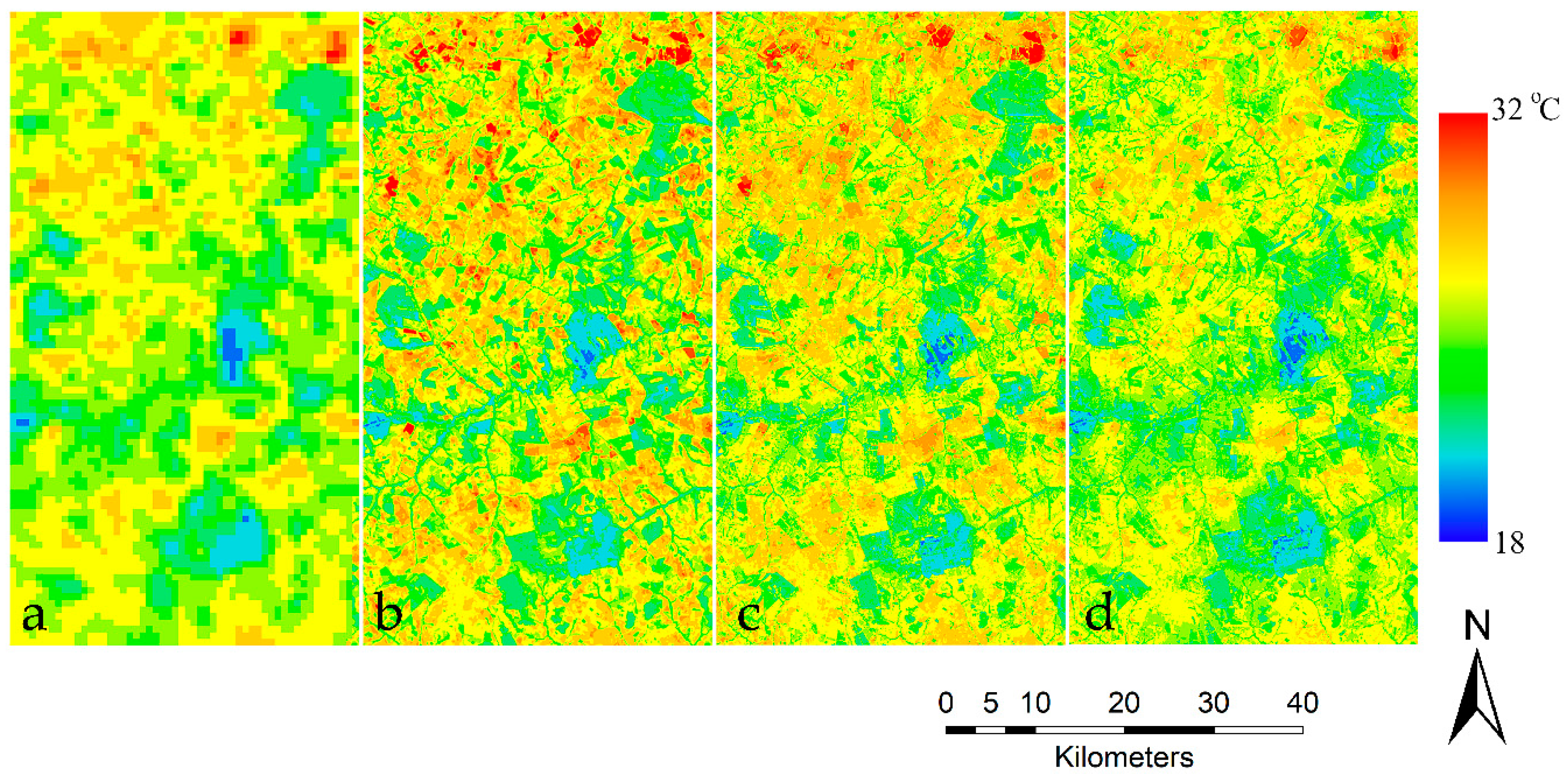
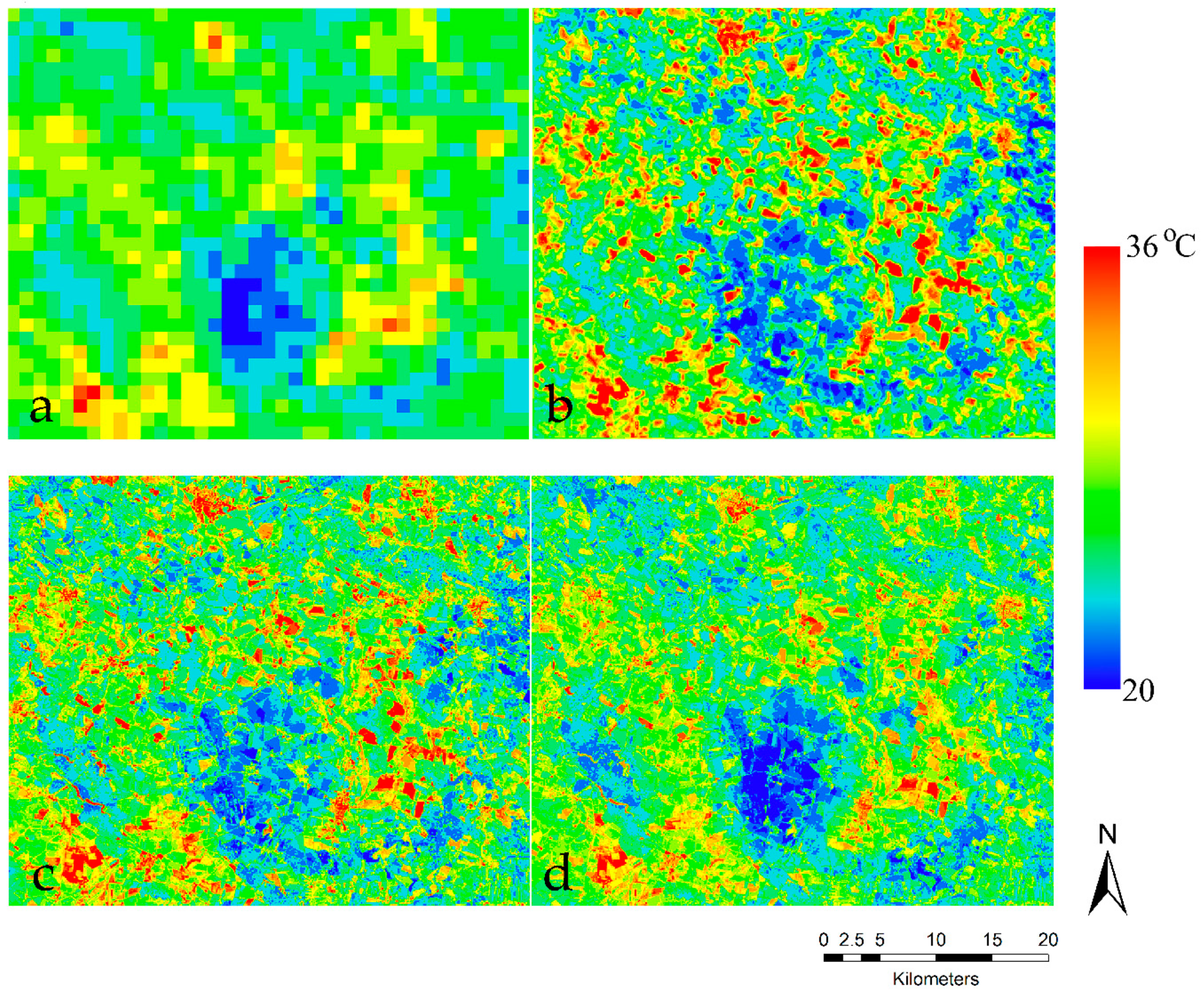
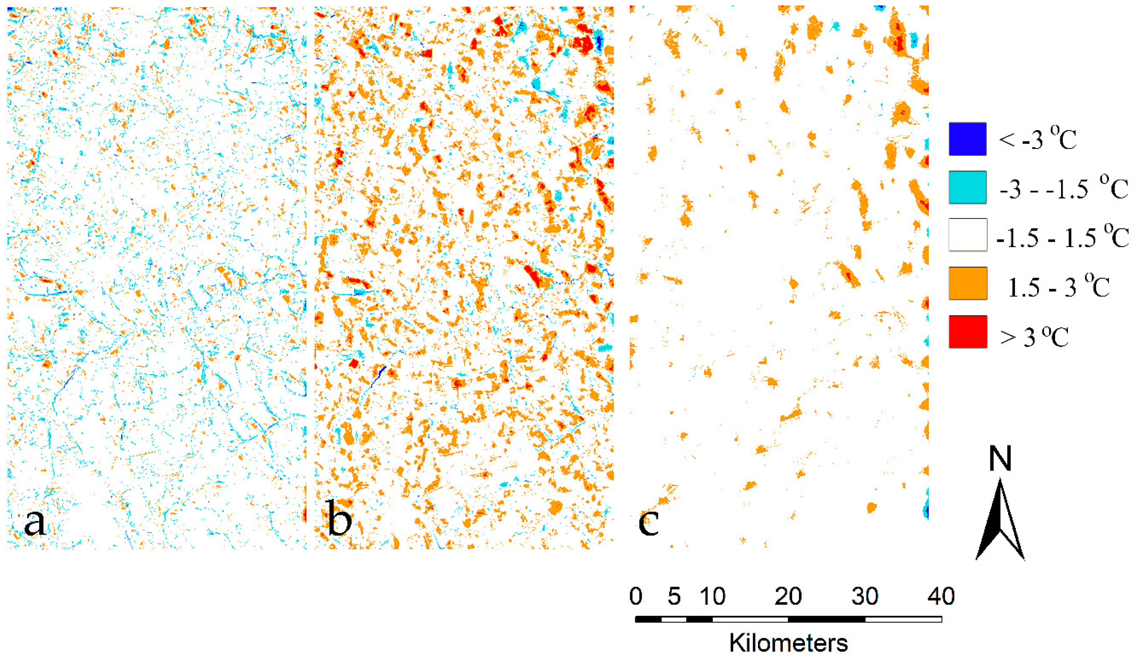
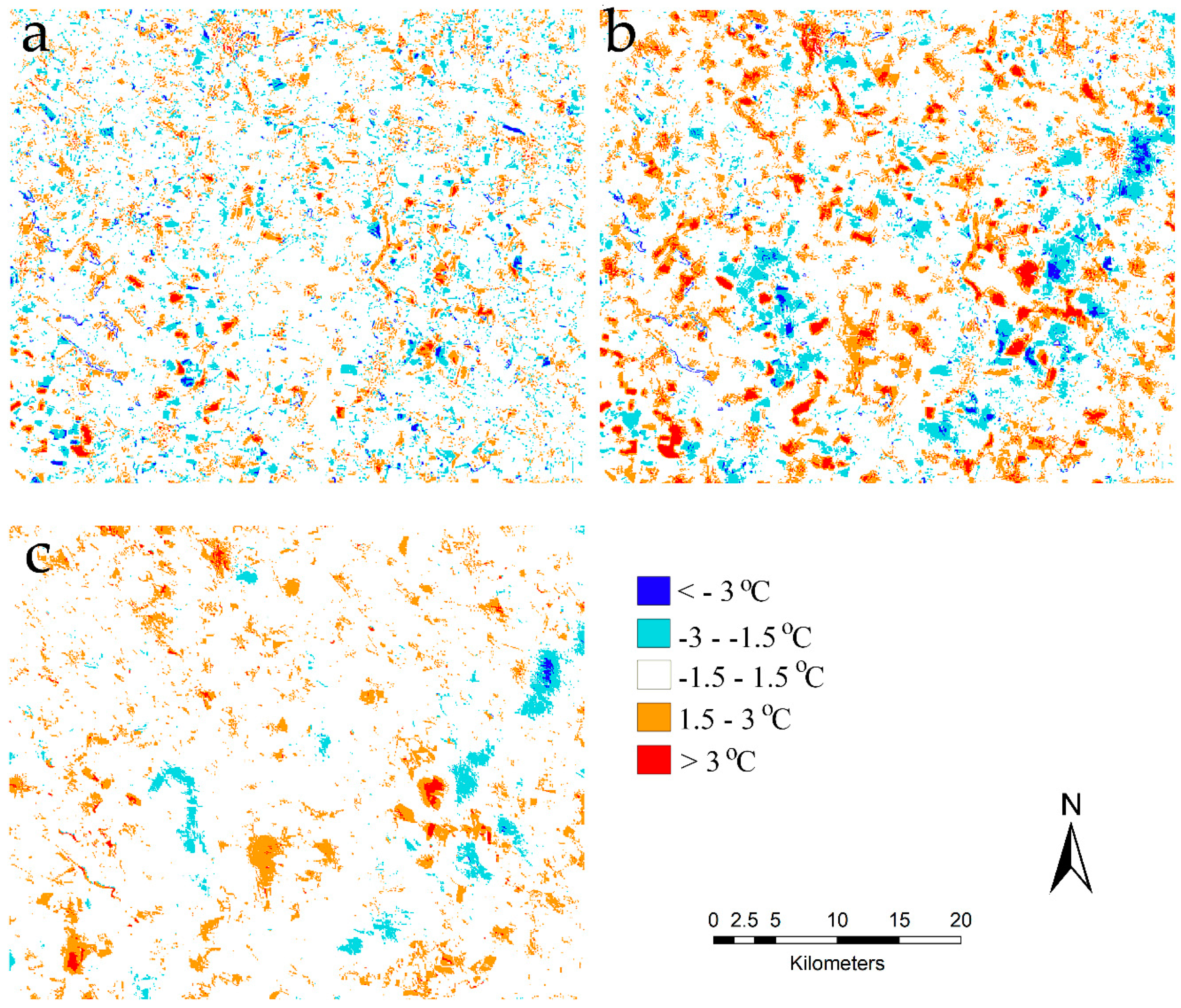
3.2. TsHARP Validation

Figure 5 and Figure 6 present the results of sharpening the 960-m resolution BT images from both aggregated Landsat 8 (TsHARPLandsat) and Sentinel-3 (TsHARPSentinel) to 60 m, alongside the ‘original’ coarse resolution image and the original Landsat 8 scene at 60 m, for Sites 1 and 2, respectively (see Figure 3 for the RGB and false color images of the sites). A visual qualitative assessment reveals that the spatial distribution of the reference image and disaggregated images showed a similar spatial distribution both when using a single (Landsat 8) platform and when using two platforms for the sharpening (Sentinel-2 and 3) and comparing the results to a third platform (Landsat 8). The maps were comparable in regions with high NDVI values, and the sharpened thermal maps showed more spatial detail than the coarse resolution BT imagery. However, the thermal maps obtained from a single platform demonstrated a much higher contrast between low and high temperatures compared to the reference image.
The TsHARPLandsat and TsHARPSentinel images were compared with the reference BT images at a 60-m resolution by computing the error difference (reference BT minus downscaled BT). Maps of the differences between the three images (the two sharpened temperatures TsHARPLandsat minus TsHARPSentinel and the Landsat reference image) for Sites 1 and 2, are presented in Figure 7 and Figure 8, respectively. In Site 1, both TsHARPLandsat and TsHARPSentinel imagery underestimated the temperature over forests and dense vegetation and overestimated the temperature over sparse vegetation fields and bare soils compared with the reference temperature. Differences >3 °C were observed in 0.09% of the area (1,283 pixels out of a total of 1,357,185 pixels in the scene) for TsHARPLandsat, and, in 7.2% of the area (98,216 pixels), the errors ranged from 1.5 to 3 °C, mostly along the borders of fields and riparian areas. This can be explained by the high correlation between BT and NDVI (Figure 7a). Agam et al. [21] reported that sharpening of homogeneously vegetated areas results in smaller errors due to the accurate fitting of the BT-NDVI regression model. For TsHARPSentinel errors > 3 °C were observed in 1.4% of the area (19,128 pixels) and errors ranging from 1.5-3 °C were observed in 20% of the area (270,511 pixels) (Figure 7b). This is likely due to loss of accuracy between different satellite platforms. Over this site, the Sentinel-based sharpened temperatures were mostly lower than those from TsHARPLandsat (Figure 7c).
Sharpening over Site 2 yielded less accurate (±3 °C) temperatures for both TsHARPLandsat and TsHARPSentinel. The lowest errors were found over agricultural landscapes for both platforms and sites. However, densely vegetated areas and bare soils resulted in larger errors due to the variation in NDVI values in different land covers. In this case as well, most errors were generally along the borders of fields and riparian areas.
The error statistics analysis indicates that the accuracy of the sharpening algorithm decreases as the target resolution becomes finer (Table 3), i.e., that the greater the difference between the original resolution and the target resolution becomes, the greater the errors. Agam et al. [17] and Essa et al. [47] also observed a decrease in accuracy with a finer resolution due to the increasing degree of subpixel variability. RMSE for TsHARPLandsat ranged from 0.68–0.83 °C and 0.85–1.17 °C, for Sites 1 and 2, respectively. The results of RMSE for TsHARPLandsat are comparable with the results from Agam et al. [17] where RMSE ranged between 0.67 and 1.39 °C, depending on the date and sensor. At both sites, BT obtained from TsHARPSentinel was less accurate with RMSE ranging from 1.1–1.5 °C. The bias of TsHARPLandsat was small and negative for Site 1, which signifies an overestimation of the sharpened temperature. The bias of TsHARPSentinel indicates that the sharpened temperature was considerably lower than the reference temperature for both sites. The MAEs for TsHARPLandsat compared to the reference BTs were also lower than for TsHARPSentinel. Compared to TsHARPLandsat, the MAE for TsHARPSentinel was higher by ~0.3 °C for Site 1 and by ~0.2 °C for Site 2 at 60-m spatial resolution. The R2 values for TsHARPSentinel were always less than those estimated for Landsat-8 data.
An overall weaker performance was observed for Site 2 in comparison to Site 1 (Table 3, Figure 8). This is likely due to the weaker correlation between BT and NDVI for Site 2. The potential limitation of using NDVI-based sharpening approaches for agricultural areas was shown by Karnieli et al. [28]. The authors suggested that, at high latitude regions, where plant growth is limited by availability of energy rather than by availability of water, the NDVI-BT correlation is positive. Being located at 50 N latitude, this may feature an additional explanation to the larger errors observed for Site 2.
Most TsHARP research is based on disaggregating MODIS, ASTER, or Landsat images from TIR to VNIR resolutions. Most of these studies have tested the sharpening using the same satellite platform. Only a few of them attempted to sharpen thermal infrared images using multiple platforms [15,20,22,40,43,44]. Mukherjee et al. [25] pointed out that using TsHARP to downscale a MODIS image from 1000 m to 250 m resulted in an RMSE of about 1.59 °C and R2 = 0.82, while downscaling aggregated Landsat 7 from 960 to 120 m yielded an error of 0.78 °C. Our results are consistent with studies by Bisquert et al. (2016a) for whom RMSE values ranged from ± 1.6-± 1.7 °C using one Landsat platform and ±1.8-±2.1 °C using MODIS versus Landsat satellites.
Lastly, to emphasize the advantage of TsHARP over a simple resampling, the Sentinel-3 coarse resolution images for both sites were resampled to 60 m without applying a sharpening algorithm and compared to the Landsat reference scenes (Figure 9).
The resulting lower R2 (0.53 vs. 0.75 and 0.30 vs. 0.65, for Sites 1 and 2, respectively) indicates that TsHARP outperforms a simple sharpening. One should also bear in mind the possibility that the errors obtained are, in fact, smaller than the ones reported in this paper. The lack of ground measurements prevents us from determining whether the Sentinel-3 or the Landsat-8 thermal images better agree with the actual surface temperatures. Thus, it is possible that we compared the TsHARP results to a less accurate reference. This remains an open question.

4. Conclusions

The mean absolute differences between Sentinel-3 and Landsat 8 BT images were up to 1 °C in all six sites, with the Sentinel-3 temperatures being typically higher. The smallest errors were found for homogeneous and relatively flat regions despite the time difference between image acquisitions. In comparative studies, such as the one presented in this paper, it is possible to intercalibrate between these two sensors when needed.
Applying TsHARP on Sentinel-3 BT data using Sentinel-2 VNIR data resulted in mean absolute errors of ~1 °C, with errors increasing as the difference between the native and the target resolutions increases. Part of the error is attributed to the discrepancy between the BT images acquired by the two platforms. This is reflected by the smaller errors observed when sharpening was applied on synthetic-aggregated Landsat-8 BT images, with errors ranging between 0.53 and 0.87 °C. These results show the potential for sharpening Sentinel-3 BT images using Sentinel-2 VNIR data for a range of applications. Further research is needed to test additional sites and conditions, and potentially additional sharpening methods, which can be applied to the Sentinel platforms.

Author Contributions

The contribution of the authors include: conceptualization—N.A., A.K., and Y.C. Methodology—N.A. and W.P.K. Software—H.H. and N.P. Validation—H.H. Formal analysis—H.H. and N.P. Writing—original draft preparation, H.H. Writing—review and editing, Y.C., A.K., W.P.K., and N.A. Visualization—H.H., Y.C., A.K., and N.A. Funding acquisition—Y.C., N.A., and A.K.

Funding

The Israel Ministry of Agriculture and Rural Development (Eugene Kandel Knowledge Centers) as part of the program Precision agriculture: Development of systems to improve resources application in the field supported this research (contract No. 235/16). The European Union’s Horizon 2020 Research and Innovation Program “Improving Future Ecosystem Benefits through Earth Observations” (Eco-potential) under grant agreement No. 641762 also partly supported this research.

Conflicts of Interest

The authors declare no conflict of interest.

References

  1. Moran, M.S.; Peters-Lidard, C.D.; Watts, J.M.; McElroy, S. Estimating soil moisture at the watershed scale with satellite-based radar and land surface models. Can. J. Remote Sens. 2004, 30, 805–826. [Google Scholar] [CrossRef] [Green Version]
  2. Sandholt, I.; Rasmussen, K.; Andersen, J. A simple interpretation of the surface temperature/vegetation index space for assessment of surface moisture status. Remote Sens. Environ. 2002, 79, 213–224. [Google Scholar] [CrossRef]
  3. Carlson, T. An Overview of the “Triangle Method” for Estimating Surface Evapotranspiration and Soil Moisture from Satellite Imagery. Sensors 2007, 7, 1612–1629. [Google Scholar] [CrossRef]
  4. Qin, Z.; Berliner, P.; Karnieli, A. Micrometeorological modeling to understand the thermal anomaly in the sand dunes across the Israel–Egypt border. J. Arid Environ. 2002, 51, 281–318. [Google Scholar] [CrossRef]
  5. Tang, R.; Li, Z.-L.; Tang, B. An application of the Ts–VI triangle method with enhanced edges determination for evapotranspiration estimation from MODIS data in arid and semi-arid regions: Implementation and validation. Remote Sens. Environ. 2010, 114, 540–551. [Google Scholar] [CrossRef]
  6. Phiri, D.; Morgenroth, J. Developments in Landsat Land Cover Classification Methods: A Review. Remote Sens. 2017, 9, 967. [Google Scholar] [CrossRef]
  7. Kustas, W.P.; Norman, J.M.; Anderson, M.C.; French, A.N. Estimating subpixel surface temperatures and energy fluxes from the vegetation index–radiometric temperature relationship. Remote Sens. Environ. 2003, 85, 429–440. [Google Scholar] [CrossRef]
  8. Chen, Y.; Zhan, W.; Quan, J.; Zhou, J.; Zhu, X.; Sun, H. Disaggregation of Remotely Sensed Land Surface Temperature: A Generalized Paradigm. IEEE Trans. Geosci. Remote Sens. 2014, 52, 5952–5965. [Google Scholar] [CrossRef]
  9. Ha, W.; Gowda, P.H.; Howell, T.A. A review of downscaling methods for remote sensing-based irrigation management: part I. Irrig. Sci. 2013, 31, 831–850. [Google Scholar] [CrossRef]
  10. Ha, W.; Gowda, P.H.; Howell, T.A. A review of potential image fusion methods for remote sensing-based irrigation management: part II. Irrig. Sci. 2013, 31, 851–869. [Google Scholar] [CrossRef]
  11. Zhan, W.; Chen, Y.; Zhou, J.; Wang, J.; Liu, W.; Voogt, J.; Zhu, X.; Quan, J.; Li, J. Disaggregation of remotely sensed land surface temperature: Literature survey, taxonomy, issues, and caveats. Remote Sens. Environ. 2013, 131, 119–139. [Google Scholar] [CrossRef]
  12. Mitraka, Z.; Chrysoulakis, N.; Doxani, G.; Del Frate, F.; Berger, M. Urban Surface Temperature Time Series Estimation at the Local Scale by Spatial-Spectral Unmixing of Satellite Observations. Remote Sens. 2015, 7, 4139–4156. [Google Scholar] [CrossRef] [Green Version]
  13. Song, X.; Zhao, Y. Study on component temperatures inversion using satellite remotely sensed data. Int. J. Remote Sens. 2007, 28, 2567–2579. [Google Scholar] [CrossRef]
  14. Zhang, H.K.; Roy, D.P.; Yan, L.; Li, Z.; Huang, H.; Vermote, E.; Skakun, S.; Roger, J.-C. Characterization of Sentinel-2A and Landsat-8 top of atmosphere, surface, and nadir BRDF adjusted reflectance and NDVI differences. Remote Sens. Environ. 2018, 215, 482–494. [Google Scholar] [CrossRef]
  15. Gao, F.; Masek, J.; Schwaller, M.; Hall, F. On the blending of the Landsat and MODIS surface reflectance: predicting daily Landsat surface reflectance. IEEE Trans. Geosci. Remote Sens. 2006, 44, 2207–2218. [Google Scholar]
  16. Agam, N.; Kustas, W.P.; Anderson, M.C.; Li, F.; Colaizzi, P.D. Utility of thermal sharpening over Texas high plains irrigated agricultural fields. J. Geophys. Res. 2007, 112, D19110. [Google Scholar] [CrossRef]
  17. Agam, N.; Kustas, W.P.; Anderson, M.C.; Li, F.; Neale, C.M.U. A vegetation index based technique for spatial sharpening of thermal imagery. Remote Sens. Environ. 2007, 107, 545–558. [Google Scholar] [CrossRef]
  18. Yang, G.; Pu, R.; Huang, W.; Wang, J.; Zhao, C. A Novel Method to Estimate Subpixel Temperature by Fusing Solar-Reflective and Thermal-Infrared Remote-Sensing Data With an Artificial Neural Network. IEEE Trans. Geosci. Remote Sens. 2010, 48, 2170–2178. [Google Scholar] [CrossRef]
  19. Gao, F.; Kustas, W.; Anderson, M. A Data Mining Approach for Sharpening Thermal Satellite Imagery over Land. Remote Sens. 2012, 4, 3287–3319. [Google Scholar] [CrossRef] [Green Version]
  20. Bindhu, V.M.; Narasimhan, B.; Sudheer, K.P. Development and verification of a non-linear disaggregation method (NL-DisTrad) to downscale MODIS land surface temperature to the spatial scale of Landsat thermal data to estimate evapotranspiration. Remote Sens. Environ. 2013, 135, 118–129. [Google Scholar] [CrossRef]
  21. Agam, N.; Kustas, W.P.; Anderson, M.C.; Li, F.; Colaizzi, P.D. Utility of thermal image sharpening for monitoring field-scale evapotranspiration over rainfed and irrigated agricultural regions. Geophys. Res. Lett. 2008, 35, L02402. [Google Scholar] [CrossRef]
  22. Bisquert, M.; Sánchez, J.M.; López-Urrea, R.; Caselles, V. Estimating high resolution evapotranspiration from disaggregated thermal images. Remote Sens. Environ. 2016, 187, 423–433. [Google Scholar] [CrossRef]
  23. Chen, X.; Li, W.; Chen, J.; Rao, Y.; Yamaguchi, Y. A Combination of TsHARP and Thin Plate Spline Interpolation for Spatial Sharpening of Thermal Imagery. Remote Sens. 2014, 6, 2845–2863. [Google Scholar] [CrossRef] [Green Version]
  24. Jeganathan, C.; Hamm, N.A.S.; Mukherjee, S.; Atkinson, P.M.; Raju, P.L.N.; Dadhwal, V.K. Evaluating a thermal image sharpening model over a mixed agricultural landscape in India. Int. J. Appl. Earth Obs. Geoinformation 2011, 13, 178–191. [Google Scholar] [CrossRef]
  25. Mukherjee, S.; Joshi, P.K.; Garg, R.D. A comparison of different regression models for downscaling Landsat and MODIS land surface temperature images over heterogeneous landscape. Adv. Space Res. 2014, 54, 655–669. [Google Scholar] [CrossRef]
  26. Duan, S.-B.; Li, Z.-L. Spatial Downscaling of MODIS Land Surface Temperatures Using Geographically Weighted Regression: Case Study in Northern China. IEEE Trans. Geosci. Remote Sens. 2016, 54, 6458–6469. [Google Scholar] [CrossRef]
  27. Bisquert, M.; Sanchez, J.M.; Caselles, V. Evaluation of Disaggregation Methods for Downscaling MODIS Land Surface Temperature to Landsat Spatial Resolution in Barrax Test Site. IEEE J. Sel. Top. Appl. Earth Obs. Remote Sens. 2016, 9, 1430–1438. [Google Scholar] [CrossRef]
  28. Karnieli, A.; Agam, N.; Pinker, R.T.; Anderson, M.; Imhoff, M.L.; Gutman, G.G.; Panov, N.; Goldberg, A. Use of NDVI and Land Surface Temperature for Drought Assessment: Merits and Limitations. J. Clim. 2010, 23, 618–633. [Google Scholar] [CrossRef]
  29. Karnieli, A.; Bayasgalan, M.; Bayarjargal, Y.; Agam, N.; Khudulmur, S.; Tucker, C.J. Comments on the use of the Vegetation Health Index over Mongolia. Int. J. Remote Sens. 2006, 27, 2017–2024. [Google Scholar] [CrossRef]
  30. Malenovsky, Z.; Rott, H.; Cihlar, J.; Schaepman, M.E.; Garcia-Santos, G.; Fernandes, R.; Berger, M. Sentinels for science: Potential of Sentinel-1, -2, and -3 missions for scientific observations of ocean, cryosphere, and land. Remote Sens. Environ. 2012, 120, 91–101. [Google Scholar] [CrossRef]
  31. Torres, R.; Snoeij, P.; Geudtner, D.; Bibby, D.; Davidson, M.; Attema, E.; Potin, P.; Rommen, B.; Floury, N.; Brown, M.; et al. GMES Sentinel-1 mission. Remote Sens. Environ. 2012, 120, 9–24. [Google Scholar] [CrossRef]
  32. Guzinski, R.; Nieto, H. Evaluating the feasibility of using Sentinel-2 and Sentinel-3 satellites for high-resolution evapotranspiration estimations. Remote Sens. Environ. 2019, 221, 157–172. [Google Scholar] [CrossRef]
  33. Choudhury, B.; Ahmed, N.; Idso, S.; Reginato, R.; Daughtry, C. Relations between evaporation coefficients and vegetation indices studied by model simulations. Remote Sens. Environ. 1994, 50, 1–17. [Google Scholar] [CrossRef]
  34. Yu, X.; Guo, X.; Wu, Z. Land Surface Temperature Retrieval from Landsat 8 TIRS—Comparison between Radiative Transfer Equation-Based Method, Split Window Algorithm and Single Channel Method. Remote Sens. 2014, 6, 9829–9852. [Google Scholar] [CrossRef]
  35. Fasbender, D.; Radoux, J.; Bogaert, P. Bayesian Data Fusion for Adaptable Image Pansharpening. IEEE Trans. Geosci. Remote Sens. 2008, 46, 1847–1857. [Google Scholar] [CrossRef]
  36. Kottek, M.; Grieser, J.; Beck, C.; Rudolf, B.; Rubel, F. World Map of the Köppen-Geiger climate classification updated. Meteorol. Z. 2006, 15, 259–263. [Google Scholar] [CrossRef]
  37. Schmidt, G.L.; Jenkerson, C.B.; Masek, J.; Vermote, E.; Gao, F. Landsat Ecosystem Disturbance Adaptive Processing System (LEDAPS) Algorithm Description; US Geological Survey: Reston, VA, USA, 2013; p. 17.
  38. Richter, R. A spatially adaptive fast atmospheric correction algorithm. Int. J. Remote Sens. 1996, 17, 1201–1214. [Google Scholar] [CrossRef]
  39. Louis, J.; Debaecker, V.; Pflug, B.; Main-Knorn, M.; Bieniarz, J.; Mueller-Wilm, U.; Gascon, F. Sentinel-2 SEN2COR: L2A Processor for Users. In Living Planet Symposium; Ouwehand, L., Ed.; European Space Agency: Prague, Czech Republic, 2016; pp. 1–8. [Google Scholar]
  40. Willmott, C.J. Some comments on the evaluation of model performance. Bull. Am. Meteorol. Soc. 1982, 63, 1309–1313. [Google Scholar] [CrossRef]
  41. Essa, W.; Verbeiren, B.; van der Kwast, J.; Batelaan, O. Improved DisTrad for Downscaling Thermal MODIS Imagery over Urban Areas. Remote Sens. 2017, 9, 1243. [Google Scholar] [CrossRef]
  42. Liu, Y.; Hiyama, T.; Yamaguchi, Y. Scaling of land surface temperature using satellite data: A case examination on ASTER and MODIS products over a heterogeneous terrain area. Remote Sens. Environ. 2006, 105, 115–128. [Google Scholar] [CrossRef]
  43. Merlin, O.; Duchemin, B.; Hagolle, O.; Jacob, F.; Coudert, B.; Chehbouni, G.; Dedieu, G.; Garatuza, J.; Kerr, Y. Disaggregation of MODIS surface temperature over an agricultural area using a time series of Formosat-2 images. Remote Sens. Environ. 2010, 114, 2500–2512. [Google Scholar] [CrossRef] [Green Version]
  44. Weng, Q.; Fu, P.; Gao, F. Generating daily land surface temperature at Landsat resolution by fusing Landsat and MODIS data. Remote Sens. Environ. 2014, 145, 55–67. [Google Scholar] [CrossRef]
  45. Brown, M.E.; Pinzon, J.E.; Didan, K.; Morisette, J.T.; Tucker, C.J. Evaluation of the consistency of long-term NDVI time series derived from AVHRR,SPOT-vegetation, SeaWiFS, MODIS, and Landsat ETM+ sensors. IEEE Trans. Geosci. Remote Sens. 2006, 44, 1787–1793. [Google Scholar] [CrossRef]
  46. Stathopoulou, M.; Cartalis, C. Downscaling AVHRR land surface temperatures for improved surface urban heat island intensity estimation. Remote Sens. Environ. 2009, 113, 2592–2605. [Google Scholar] [CrossRef]
  47. Essa, W.; Verbeiren, B.; van der Kwast, J.; Van de Voorde, T.; Batelaan, O. Evaluation of the DisTrad thermal sharpening methodology for urban areas. Int. J. Appl. Earth Obs. Geoinformation 2012, 19, 163–172. [Google Scholar] [CrossRef]
Figure 1. Data processing flow chart.
Remotesensing 11 02304 g001
Figure 2. Landsat 8 OLI color-infrared images at 30-m spatial resolution for: (a) Site 1, image acquired on 13 July 2017. (b) Site 2, image acquired on 20 June 2017. (c) Site 3, image acquired on 16 July 2017. (d) Site 4, image acquired on 16 July 2017. (e) Site 5, image acquired on 9 July 2017, and (f) Site 6 image acquired on 17 October 2017. The outlines in Panels b and e delineate the analyzed areas.
Remotesensing 11 02304 g002
Figure 3. Areas used for sharpening and NDVI calibration in natural and false colors. (a) Site 1, image collected on 13 July, 2017, and (b) Site 2, image collected on 20 June, 2017.
Remotesensing 11 02304 g003
Figure 4. Relationship between two BTs derived from Landsat 8 and Sentinel-3 at a coarse spatial resolution (960 m) for: (a) Site 1, (b) site 2, (c) site 3, (d) site 4, (e) site 5, and (f) site 6. The black line represents the regression line. The dashed red line is the graph 1:1 line.
Remotesensing 11 02304 g004
Figure 5. Sharpening brightness temperature images from a 960-m to a 60-m resolution for Site 1. (a) Sentinel-3 BT at 960 m. (b) Reference Landsat 8 BT at 60 m. (c) Sharpened to 60-m BT derived from applying TsHARP to aggregated Landsat 8 using Landsat 8 60-m Normalized Difference Vegetation Index (NDVI). (d) Sharpened to 60-m BT derived from applying TsHARP to Sentinel-3 using Sentinel-2 60-m NDVI.
Remotesensing 11 02304 g005
Figure 6. Sharpening BT images from a 960-m to 60-m resolution for Site 2. (a) Sentinel-3 BT at 960 m. (b) Reference Landsat 8 BT at 60 m. (c) Sharpened to 60-m BT derived from applying TsHARP to aggregated Landsat 8 using Landsat 8 60-m NDVI. (d) Sharpened to 60-m BT derived from applying TsHARP to Sentinel-3 using Sentinel-2 60-m NDVI.
Remotesensing 11 02304 g006
Figure 7. Residuals maps of (a) TsHARPLandsat at a 60-m spatial resolution. (b) TsHARPSentinel at a 60-m spatial resolution, and (c) difference between TsHARPLandsat and TsHARPSentinel for Site 1.
Remotesensing 11 02304 g007
Figure 8. Residuals maps of (a) TsHARPLandsat at a 60-m spatial resolution. (b) TsHARPSentinel at a 60-m spatial resolution, and (c) difference between TsHARPLandsat and TsHARPSentinel for Site 2.
Remotesensing 11 02304 g008
Figure 9. Relationship between two reference Landsat 8 and resampled Sentinel-3 BTs at a fine spatial resolution (60 m) for (a) Site 1 and (b) Site 2. The solid black line represents the regression line and the dashed red line is the 1:1 line.
Remotesensing 11 02304 g009
Table 1. List of study sites and Landsat 8, Sentinel-3, and Sentinel-2 images used in this study.
SiteAcquisition DateLocationCoordinatesLandsat 8Sentinel-3Sentinel-2
Path/RowOverpass Time (Local Time)
113-Jul-17Campo Grande, Brazil 20.13°S, 53.32°W224/749:349:349:51
220-Jun-17Podebrady, Czech Republic 50.14°N, 15.15°E191/2511:5011:5012:00
316-Jul-17Omaha, Iowa - Nebraska, USA 41.45°N, 96.1°W28/3112:0512:00-
416-Jul-17Sacramento, CA, USA38.54°N, 121.39°W44/3311:4511:44-
59-Jul-17Sacramento, CA, USA37.28°N, 120.35°W43/3411:3911:25-
617-Oct-17Madhya Pradesh District, India 23.6°N, 79.33°E114/4411:0811:08-
Table 2. Quantitative analysis of the differences between the simulated Landsat 8 thermal data and Sentinel-3 TM data at a coarse spatial resolution. The statistics include: the regression coefficients slope and intercept, coefficient of determination (R2), root mean square error (RMSE), mean absolute error (MAE), mean bias (Bias = Sentinel-3 (S3) minus Landsat 8 (L8)), and normalized RMSE (nRMSE).
SitesDate of Image AcquisitionAcquisition Time Difference (L8–S3) (min)Intercept (°C)SlopeR2RMSEMAEBiasnRMSE
113-Jul-1700.750.990.850.920.720.427.4%
220-Jun-1701.730.960.851.110.830.554.5%
316-Jul-1750.970.990.920.710.610.575.9%
416-Jul-1701.600.980.961.281.00.714.2%
59-Jul-17150.101.00.931.381.00.184.4%
617-Oct-1701.410.980.951.080.900.805.8%
Table 3. Statistics of the disaggregated thermal maps in comparison with the referenced thermal imagery.
Site 1Site 2
240 m120 m60 m240 m120 m60 m
MAETsHARPLandsat0.530.590.640.640.780.87
TsHARPSentinel0.880.920.950.921.021.09
R2TsHARPLandsat 0.890.860.840.830.790.77
TsHARPSentinel 0.800.780.760.690.670.65
RMSETsHARPLandsat 0.680.770.830.851.051.17
TsHARPSentinel 1.121.171.201.201.341.45
BIASTsHARPLandsat -0.003-0.004-0.0040.0070.0090.013
TsHARPSentinel 0.630.630.630.270.270.27

