1. Introduction
The average growth of magma bodies is commonly slow, with long-term values leading to inflation rates of up to a few centimeters annually [
1,
2,
3]. Large magma chambers and plutons are heterogeneous bodies [
4] and are believed to grow by incremental episodes that cause accumulation of intrusive bodies in the Earth’s crust [
5,
6]. Magma chambers are thought to be inherently unstable [
7] and may re-organize, rapidly change and fluctuate, and can be associated with variable inflation episodes observed at the surface. Identifying and understanding such mass movements and the formation of major magma bodies are of great interest for scientists and society, as they allow an understanding of volcanic unrest, the formation of thickened crust [
8], and because they may feed large and possibly caldera-forming eruptions [
9,
10].
Mobilization of volumes of magma in the crust and the (episodic) growth of magma bodies can be effectively investigated by identification of gravity anomalies and deformation measurements, but only a few examples exist worldwide where (i) large-dimension doming was identified and (ii) monitored by multi-parametric data. Some of the most prominent examples are found in South America, where the three large-scale sites of doming identified are Laguna del Maule, Lazufre, and Uturuncu [
11]. These key global sites are located in the central and southern Andes, also showing unique evidence for ignimbrite-forming eruptions in geologic history [
12] and hosting the largest partial melting zones known (the Altiplano–Puna Mush Body and the Southern Puna Magma Body) [
12]. Previous studies have revealed distinct geophysical anomalies in the upper, middle, and lower crust that are possibly associated with multiple, distinct magma ponding levels and/or hydrothermal fluids [
8]. The sites at Laguna del Maule, Lazufre, and Uturuncu are all subject to “large caldera-scale” inflation [
13] and are amongst the first that have been identified in recent years (
Figure 1c). In fact, satellite geodetic data reveal that inflation has been ongoing at Uturuncu since at least 1992 [
14], and at Laguna del Maule and Lazufre the inflation began in 2004 [
15] and 1998 [
16,
17,
18], respectively. Here, we report on gravimetric and deformation data from another site showing major inflation and possible magma accumulation that was recently identified in the Southern Andes. Our study was initiated by seismic records at the poorly studied Domuyo Volcanic Center (DVC), Argentina, and emphasizes the relevance of incremental crustal growth and sudden unrest activity, even at those volcanoes that have had no historical eruptive activity. This paper is organized as follows: First, we introduce the poorly known volcanic center and describe the data and methods used. We combine satellite remote sensing with field campaign data, by investigating gravimetric and magnetic data, and interferometric synthetic aperture radar (InSAR) deformation maps, to derive a geological model of the structure of the magmatic-hydrothermal system at depth, and we compare this to the geomorphology at the surface.
2. Tectonic Setting and Geology of the Domuyo Volcanic Center
The Domuyo Volcanic Center (DVC) (36°37’ S–70°26’ W) is a dome complex 4702 m high located in the southern Central Andes of Argentina. This volcanic center (SI_VNUM 357067 [
19]) hosts a number of dacitic lava domes and monogenetic basaltic centers and is the site of intense geothermal activity associated with regional extensional and transtensional structures [
20]. The NE flank of the summit is truncated by an amphitheater 4 km wide that hosts a central dome-like structure. The DVC occupies a retroarc position with respect to the active volcanic front that also formed the Chillán, Antuco, Sierra Velluda, Copahue, and Llaima volcanoes, see
Figure 1a. This retroarc position is shared with other silicic caldera and dome complexes, such as the Calabozos caldera, Laguna del Maule Volcanic center, the Tilhue dome, and the Campo Volcánico Puelche, that have been petrologically interpreted as products of crustal melting under an extensional regime [
21,
22,
23,
24]. Limited amounts of mantle-derived materials are mixed at this western retroarc position with crustal-derived products conforming basaltic floods and isolated central volcanoes [
22]. Extensional structures controlling the emplacement of Quaternary volcanic products have been described that affect the western sector of the Malargüe fold and thrust belt [
25], located between 35 and 38°S, and form a series of extensional valleys subject to material deposition (so-called depocenters), which are the troughs of the Las Loicas, Loncopué, and Bío Aluminé (
Figure 1a). The La/Yb ratios in the eastern Payenia volcanic field retroarc products have provided insights regarding the crustal thicknesses in the region and reveal a longitudinal zone of attenuated crustal thickness of 33–35 km, which is compatible with the extensional conditions determined from structural and geochemical studies [
26].
This extensional setting has been partly explained by tearing of the subducted Nazca Plate 4–5 My ago [
27]. This tearing affected the southern part of the subducted plate at around 38°S and produced a pronounced step that controls the transfer zone between the Loncopué and Las Loicas troughs [
28]. Asthenospheric material ascended through the fractures on the subducted oceanic floor and produced distinct mantle upwellings, decompression, and fed foreland basaltic floods of the Payenia, Tromen, and Auca Mahuida volcanic fields, as has been visualized through magnetotelluric and gravimetric geoid data [
29,
30]. The DVC and its new episode of unrest episode may be a consequence of such upwellings.
Available radiometric datasets allow inference of an eruptive period at the DVC that extends from 2.5 to 0.11 My [
31,
32,
33,
34,
35]. During this period, two distinct eruptive-compositional stages were identified. The first occurred from the Late Pliocene to Early Pleistocene and had a dominant calc-alkaline signature with andesitic and explosive eruptions that led to widespread pyroclastic fluxes. The second stage occurred from the Middle to Upper Pleistocene and was associated with the final development of a complex monogenetic dome structure, principally in the southwest of the Domuyo. Until recently, the DVC was considered as a dormant center.
An important characteristic of this volcanic center is its thermal activity that has been studied since the 1970s [
18,
32,
36,
37]. Most of the earlier studies have described a fault-controlled system with fumaroles, hot springs, and geysers that is associated with one of the largest advective heat fluxes measured for a single volcanic center. A possible reactivation of this volcanic center was proposed [
18] considering the measured energy fluxes, which are difficult to reconcile as being the result of cooling of old magmatic systems.
Finally, neotectonic activity has been described in association with the thermal manifestations [
20,
38]. These consist mainly of normal faults associated with limited amounts of lateral slip that cut through the Early Quaternary ignimbritic facies on the western slope of the DVC. Based on geologic mapping, some of these structures were interpreted as neotectonic [
20,
39], but modern multi-parametric monitoring and analyses of the unrest episode has not been achieved yet. To define a geometric source model that can reproduce and explain the unrest pattern that has been detected over the DVC, in this work, we present an analysis of different data sets, including seismic data, interferometric synthetic aperture radar (InSAR), and gravimetric and magnetic terrestrial data, and then we develop a synthesis that also considers a surface morphology analysis. Given the constrained dimensions of the surface deformation and inferred magma reservoir beneath, we herein provide evidence that DVC is one of the largest inflation sites known in the Andes.
3. Materials and Methods
Ground-based monitoring, campaign field measurements, and satellite remote sensing were combined in this work. Here we describe the data and methods used: the seismic network, the gravimetric data, the InSAR deformation maps, the magnetic data, and morphometric surface analysis. We then provide details regarding the inversion and modeling techniques used to infer the source(s) of the observed anomalies.
3.1. Seismic Data
The timely observation of seismic signals is a key aspect of volcano monitoring [
40]. Hydrothermal activity, degasification, and fracturing or migration of magma, among other factors, generate a wide variety of seismic signals [
15,
41,
42,
43].
The seismic data presented in this work were acquired from July 2017 to March 2018 by using a network of nineteen three-component broadband seismometers (Trillium Compact and Trillium 120PA from Nanometric, Inc.) and using a sampling frequency of 200 Hz. The seismic network was further extended by two additional short-period stations located in the south of the Mendoza province (blue triangles in
Figure 1a). We also considered five Chilean stations, which are part of the International Federation of Digital Seismograph Network (FDSN), improving the azimuthal coverage (
Figure 1a). The loggers used for FDSN were Centaur and Taurus, both from Nanometrics, Inc., with five possible gain inputs that were configured to be able to register even small-scale seismic events. All 26 station records were used for locating the seismic events.
Processing was performed using the SEISAN platform [
44] and the Obspy package (
https://github.com/obspy). We first applied an automatic detection algorithm based on short-term averages over long-term averages (STA/LTA), controlled by meticulous visual observations using a multitrace module to eliminate false positives and to identify the P- and S-wave arrivals. The seismic event locations were computed using HYPOCENTER [
45,
46] and by use of a one-dimensional velocity model composed of nine layers, developed for the area of interest by Correa-Otto et al. [
47]. A seismic event database was constructed from several continuous registers, showing a cluster of events located beneath the summit and western flank of the DVC. We also calculated the Ml and Mw magnitudes. In this work, we present the events that have locations shallower than 25 km. The results are provided in map views for comparison to the other data in
Section 4.1.
3.2. InSAR Data
Since the early 1990s, the InSAR ground-surface deformation technique has become a popular tool for monitoring active volcanoes [
42], and thanks to the free availability of the European Space Agency’s Sentinel data, since 2015 the method has allowed monitoring of almost any potential volcano site worldwide [
48]. The ground-deformation observations provide useful information about eruptive cycles to assess volcanic hazards. In addition, this technique allows for making inferences of storage locations and magma conduits, and by the implementation of modeling inversions of InSAR data, it is possible to better understand the geometry and location of the deformation source [
11,
16,
49,
50].
We used radar satellite observations to assess deformation occurrence associated with a possible magma body beneath the DVC. The aim of this analysis is to construct an independent database that is compared to our geophysical field data (gravity and magnetic). We selected Sentinel-1 acquisitions that were obtained during the absence of snow, as snow coverage may strongly affect the signals [
51]. After downloading acquisitions over the snow-free target area, we processed the differential interferograms (d-InSAR) by using the Sentinel Application Platform (SNAP), freely provided by the European Space Agency (
http://step.esa.int/main/toolboxes/snap/). SNAP combines a suite of available Sentinel toolboxes and allows complex data analysis and SAR processing.
Processing follows the classic steps for obtaining deformation velocities: first, co-registration between the two images; then, Interferogram generation including flat-earth phase removal and coherence estimation; then, application of the Terrain Observation with Progressive Scans (TOPS) deburst algorithm. The topographic phase was removed using the SRTM 3-sec Digital Elevation Model (DEM), after which, multilook processing was implemented while maintaining a square pixel in which the number of looks in range was chosen to be between 4 and 12, depending on the quality of the images. A Goldstein filter was applied to filter the phase [
52]. Phase unwrapping was achieved by using SNAPHU software [
53,
54,
55]. By this, the conversion of phase to displacement was realized. We then geocoded the data by range-Doppler terrain corrections in order to provide the final products.
We used Sentinel-1 images acquired from both ascending and descending orbits. As the selection of the image pair dates was made while considering the presence of snow in the DVC during the winter season, a relatively small dataset remained. For this, we considered those pairs of small perpendicular baselines (<100 m) between two SAR images to avoid topographic artifacts and coherence loss.
Figure 2 presents the totals of the number of differential interferograms processed in this work (27). We estimated from the d-InSAR results if pronounced trend changes were present. As we found that the amount of deformation linearly increased with the temporal baseline, we assumed a linear trend, which is also in agreement with an earlier study [
56]. The deformation rate was linearized by fitting the number of fringes versus time period for the interferograms. We selected 12 interferograms (
Table 1) that showed the highest quality among the 27 data pairs processed within the 2014–2018 time period, and then we normalized the deformation rates to a 1 year period to perform the stacking process and therewith to increase the signal-to-noise ratio [
57,
58,
59,
60,
61,
62] (see
Figure 2). The aim of these deformation assessments was to generate a database that supported the gravimetric and magnetic field measurements (described in the following sections); future studies might allow more rigorous exploration of the deformation rate changes by considering time series analyses, which was beyond the scope of this work.
The selected image pairs with the best coherence are presented in
Table 1. The stacking results and the deformation pattern for the DVC are presented in
Section 4.2.
3.3. Gravimetry Data
The study of gravity anomalies in active volcanic centers allows detecting changes in density distributions at depth over different observation periods [
42]. Gravity data also can be utilized to identify low-density bodies underlying the volcanic surface that may indicate reservoirs of partial melts or hydrothermal fluids in the upper crust [
15,
63,
64,
65]. In the Andes, gravity surveys could help to identify some of the largest magma bodies at depth [
66], such as at the Uturuncu inflation site [
67].
The gravimetric data presented in this work represent a heterogeneous network made via accessible paths and roads located around the DVC, with measurements taken every 1000 m, on average, during the period of January–February 2018 (illustrated as inverted black triangles in
Figure 1b). For the gravimeter we used the CG-5 AutoGrav instrument from Scintrex, Ltd., which has a fused quartz sensor with a resolution of 1 µGal. The data were corrected for drift variations using the same reference point as the database. The complete Bouguer anomalies with the free air and Bouguer corrections applied were calculated following the classic expressions from Blakely [
68], and the observed gravity values were tied to the International Gravity Standardization Net system (1971), and the normal gravity to the station latitude, using the 1967 international ellipsoid. We considered the Earth’s curvature and applied terrain corrections according to LaFehr [
69] and Nagy [
70].
The regional trend of the Bouguer anomaly map is presented as an upward continuation up to 20 km. The resulting residual was computed by subtracting this regional map from the Bouguer anomaly map. The results are presented in
Section 4.3. We used units of milligal(s) (mGal, in cm/s
2) throughout the results and figures.
3.4. Magnetic Data
Magnetic anomalies are used to study the physical mechanisms involved in volcanic processes due to changes in the thermal and stress configuration subsurface, fluid movements, or remagnetization after eruptions or shallow magmatic emplacements. Dikes, vents, domes, and faults can be identified by significant magnetic anomalies in addition to using structural knowledge and gravimetric data over the study area [
42,
71,
72,
73,
74].
The terrestrial magnetic data were measured along with the gravimetric data during the period of January–February 2018 with a GEM GSM system (19 V7) Overhauser total field magnetometer with a sensitivity of 0.02 nT and an absolute precision of 0.1 nT.
The data were corrected for diurnal variations. The total magnetic anomaly (TMA) was computed by subtracting the international reference field value (IGRF) from the observed total field. To better analyze the magnetic anomalies, the analytic signal (AS) was computed, and a reduce-to-pole (RTP) filter was applied to the TMA with 5.12° of declination and −37.7° of inclination. The three maps, namely, TMA, RTP, and AS, are presented in
Section 4.4.
3.5. Data Modeling
Modeling was performed using simple and idealized source geometries in an attempt to constrain the reservoir location and shape [
42] and to compare/validate interpretations derived from the different data presented herein. In the following, we describe the modeling approaches used for the InSAR data and for the Bouguer gravity anomaly data.
3.5.1. Source Modeling from InSAR
We used the freely available Geodetic Bayesian Inversion Software (GBIS) [
75], which allows the estimation of optimal parameters such as the depth, geometry, and orientation of the deformation source using data from ascending and descending satellite tracks. We chose two interferograms with the best quality and similar dates from the period May 2017 to March 2018 and a temporal baseline of 300 d for the ascending track and 324 d for the descending track, respectively.
The GBIS software estimated the variance and covariance in each independent data set to reduce randomly distributed noise and also possible spatially correlated phase delays by calculating the semivariograms of each data set that were in proximity but not in a deformed area. A linear ramp was also applied to remove possible residual orbital errors or atmospheric residual delays with long wavelengths [
75]. The subsamples were computed using a quadtree of 2 × 10
−4 for the ascending data, resulting in 232 points, and a quadtree of 2.5 × 10
−4 for the descending interferogram, resulting in 82 points (see
Appendix A).
The inversion was applied using analytical solutions for an isotropic elastic half-space for different geometries: a horizontal rectangular sill [
76], a prolate spheroid [
77], a penny-shaped sill-like source [
78], a point source [
79], and, finally, a rectangular sill geometry with a strike and dip orientation [
76]. The results were obtained by performing 10
6 iterations using posterior probability density functions to constrain the input parameters for the different geometries mentioned above.
To determine the best-fit model, we considered the statistical values: RMS (root mean square of the residuals), WRSS (weighted root sum square), and the Akaike information criterion (AIC). The latter appraise the balance between complexity (number of parameters) and precision of the models [
80,
81,
82,
83].
The results are presented in
Section 4.5.1, where the best-fit modeled and measured patterns can be compared.
3.5.2. D Density Modeling from Bouguer Anomalies
We performed a 3D density modeling with IGMAS+ modeling software (Interactive Gravity and Magnetic Application System) [
83,
84,
85,
86,
87,
88,
89,
90,
91].
The procedure started by fitting the model with the residual Bouguer anomalies described in
Section 3.3, considering only a small area around the low gravity value that was expected to be the signal of the deformation source. The simple model used consisted of two bodies, one for the host rocks and the second body represented a low-density, volatile-rich reservoir that was consistent with the silicic volcanic material in the DVC. For the density contrast, we considered the results of Miller et al. [
65] for the Laguna del Maule volcanic field magmatic system, which is located 55 km to the northwest of the DVC and presents a similar magmatic geochemical signature. Miller et al. [
65] developed thermodynamic modeling and concluded that the reservoir consisted of a volatile-rich magma with 85% of melt restrained in a wholly or partially crystallized mush with a density contrast of −600 kg/m
3. In the present work, we used a density contrast of –550 kg/m
3 to fit the gravimetric contrast of almost 20 mGal.
The dimensions of the reservoir were further constrained by the dimensions obtained from GBIS modeling. Therefore, the following three-dimensional density models were ultimately considered: first, a model that fit the measured density anomaly that had a higher volume, and second, a model that followed the exact dimensions of the GBIS-modeled deformation source but resulted in a higher residual Bouguer anomaly.
The results are detailed in
Section 4.5.2, where the residuals of the calculated Bouguer anomalies and the geometries used are presented. The interpretation and conceptual model are elaborated in more detail in the discussion section of this paper.
3.6. Morphometric Analysis
Using morphometric analysis for the study of surface modification is a practice that has been used in the past few years. Many studies highlight the importance of analyzing the equilibrium state of fluvial networks to detect areas with active uplift due to tectonic processes or magmatic emplacement [
92,
93,
94,
95,
96,
97]. To decode local and regional landform responses and to analyze potential topographic changes in the area, we analyzed the drainage patterns and developed swath profiles. In particular, we studied the equilibrium states of the rivers draining the DVC to evaluate potential relief changes and the fluvial networks resulting from inflation of the area. We used the SRTM (Shuttle Radar Topography Mission) (30 m) digital elevation model to obtain swath profiles along the main courses using TopoToolbox, a set of functions for topographic analysis implemented in Matlab [
98,
99]. We extracted the watersheds that drain the DVC and selected the trunk for each basin. After separating the trunks, we extracted the swath profiles along the course until the headwaters were reached. These swath profiles condense maximum, mean, and minimum elevation data to a single chosen topographic profile. Each swath profile along a particular channel allows us to evaluate how the relief of the valley had changed in each basin.
4. Results
4.1. Seismic Data
The yellow dots and squares in
Figure 3 show the seismic activity that was shallower than 25 km and that was recorded during the period of July 2017 to March 2018 (for more details, see
Appendix B). The moment magnitudes of all of these events remained below Mw = 3. The event locations had low precision because of the low azimuthal coverage of the network used. Thus, only general characteristics should be taken into consideration when describing the seismic activity in the area from this dataset. In
Appendix B, the uncertainties in the locations of these events are presented. Therefore, even though the existence of seismic activity within the DVC area was confirmed from this dataset, only a qualitative description can be made. The activity focused on the southwestern slope of the DVC and coincided with hydrothermal and neotectonic activity [
20,
38]. Three events (yellow squares in
Figure 3) nucleate near the summit portion of the DVC. It is worth noting that the uneven distributions of the seismicity between the southern and northern slopes and western and eastern slopes of the volcanic center coincide with an identified neotectonic structure (
Figure 3).
4.2. InSAR Data
The InSAR data revealed a large deformation area centered on the DVC summit area, partially covering the geothermal locations. The deformation was detected in several independent data pairs using both satellite configurations (ascending and descending) and consisted of a circular, slightly elliptic geometry, with a main axis in the northwest–southeast direction (305° azimuth) that was approximately 20 km long with a short axis of approximately 18 km.
Figure 4 presents examples of ascending and descending interferograms for the time period between May 2017 to March 2018, indicating a maximum uplift of approximately 5 fringes that represents ~14 cm in both line-of-sight LOS directions (λ
sentinel-1 = 5.54 cm).
The selected interferograms and the resulting stacks are shown in
Figure 5. A mean deformation velocity peak of 12 cm/year is calculated from the descending and ascending interferograms. Every product presented in
Figure 5a1–a6 and the b-series corresponds to different time periods and, consequently, to different uplift magnitudes. A possible nonstationary atmosphere effect was reduced by the stacking process, although the presence of a static tropospheric delay that remained approximately constant in time could still be present after the stacking. The detected number of fringes presented over the DVC are interpreted to mainly be due to a deeper crustal deformation source.
4.3. Gravimetry Mapping Results
In
Figure 6, the Bouguer anomaly map from terrestrial data and its regional and residual maps are presented. The regional component of the Bouguer anomaly,
Figure 6b, revealed a negative anomaly with a long wavelength of ~30 km, located in the northeastern sector of the studied area that was separated from the DVC edifice.
The residual anomaly map,
Figure 6c, revealed pronounced density heterogeneities located in the upper (shallow) crust, such as an elongate positive anomaly through the Cordillera del Viento basement uplift. A negative signal was observed on the southern slope of the DVC that can be interpreted as two principal anomalies with different wavelengths placed side by side. The longest anomaly had a wavelength λ
1 = 26 km, was hosted in the lower crust, and was south of the Domuyo summit. The shorter anomaly had a wavelength λ
2 = 15 km, was shallower, and was positioned to the northeast.
4.4. Magnetic Maps
Magnetic maps are illustrated in
Figure 7 and show the total anomaly, the results of pole reduction, and the analytic signal superimposed with the neotectonic normal faults studied by Galetto et al. [
20] and the hydrothermal activity. The data revealed a concentric arrangement of anomalies that reflected the main structures segmenting the basement of the DVC. From the analysis of the reduced-to-pole and analytic signal, we can better interpret the locations of these magnetic sources. The general circular shape coincided with the InSAR deformation pattern and to the main volcanic sources (see
Appendix C for a direct comparison between the surface geology and the magnetic anomalies). We noted a positive magnetic anomaly located at the DVC, surrounded by a negative anomaly, and in turn surrounded by positive areas on the periphery. Southwest of the area (southwest of the InSAR deformation pattern, black dashed line in
Figure 7), a magnetic high was seen that coincided with the hydrothermal area, which has been previously described as due to water recirculation through a fault system [
20]. An alignment between some of the W-E and N-S structures and the magnetic anomalies was observed.
4.5. Source Modeling Results
4.5.1. Modeling from InSAR Data
To determine the best geometry modeled we considered the AIC criterion, RMS, and WRSS as were mentioned in
Section 3.5.1. The lowest AIC values corresponded to the point source model, followed by the Penny-shaped sill-like model, then the horizontal and the dipping rectangular sills, and finally the prolate spheroid source (
Table 2). These results seem to be more related to the number of parameters involved in each geometry than the precision of the residuals. However, when considering the 3D gravimetry modeling, the geometries with lowest AIC caused a misfit of the Bouguer anomaly. Moreover, it was not possible to develop a 3D density model using a point source geometry, and the small volume of the Penny-shaped sill-like located at 10 km depth could not reproduce the Bouguer anomaly.
On the other hand, the lowest RMS and WRSS values (
Table 2) corresponded to the rectangular sill sources. The dimensions of both geometries were similar and were approximately 10 × 8 km
2 (see
Appendix A), but the horizontal sill was located 0.8 km deeper than the dipping sill (6.7 km depth). To resolve which sill model better represented the deformation source, we tested both depths during modeling of gravity data, and we determined that the dipping sill better reproduced the lower anomaly. Therefore, from all of the geometries tested for the inversion, the InSAR data-set can be best explained by a rectangular sill geometry of around 7.5 × 10 km
2 and 0.5 m of opening with strike N58°E, and a dip orientation of 10° toward the west, according to the RMS and WRSS criteria and to the 3D density modeling.
From the selected geometry, the rectangular dipping sill source, we can investigate the source parameters in
Figure 8. The horizontal positions presented a high correlation with the rest of the parameters, and the strike, dip, width, and length were well constrained. Further details are presented in
Appendix A, where a summary of the parameter results for all tested sources are listed, including the complete inversion results for the rectangular dipping sill and the posterior probability density function.
In
Figure 9, the model and residual patterns can be compared to the input data. The resulting source depth was ~7 km below the surface. It is worth noting that the modeling code we used did not apply a topographic correction and that the DVC presented a pronounced relief of ~4 km above sea level, which is to be considered as the reference for all depth estimates.
4.5.2. D Modeling from Gravity Data
The Bouguer anomalies of the two models developed by fitting the measured Bouguer residuals are presented in
Figure 10. The model that better fit the measured anomaly,
Figure 10a, required a greater volume and a shallower depth of 4 km, while the model with a geometry retrieved by the InSAR modeling, shown in
Figure 10b, indicated a slightly greater depth of 6 km. The density contrast used was the same for both models (−550 kg/m
3) according to the predominant rhyolitic products. The differences between the modeled and the original Bouguer anomalies were minor but revealed short wavelength residuals in the southwest and in the east of the DVC (
Figure 10c,d). Also, the absolute values of the residuals did not exceed 5 mGal, except for the deeper body, which differed by 10 mGal for the measured minimum anomaly value.
Both geometries used for the 3D density model are presented along with the geometry of the InSAR modeling (rectangular dipping sill) in
Figure 11.
4.6. Morphometric Results
The first element that was obtained from the morphometric analysis was related to the uneven sizes of the different watersheds that drain the DVC. The western watersheds, rivers 1–4 in
Figure 12, presented systematically smaller drained areas, while the eastern, northern, and southern watersheds (rivers 5–8 in
Appendix D) showed more integrated local networks and an advanced state of maturity for the relief. Therefore, the western watersheds are thought to have evolved over unstable terrain that coincides with the inflation area indicated by the InSAR data.
The swath profiles along the trunks of basins 1 to 8 are presented in
Figure 12 and in
Appendix D. Greater differences between minima and maxima imply higher relief of the valleys and, therefore, greater incision. On the one hand, rivers 6 and 7 from the east slope were inferred to present greater levels of incision at their headwaters and are explained by lithological changes observed in the geological (
Appendix D), at approximately 2500 m altitude. On the other hand, the swath profiles from the western rivers 1–4 showed pronounced changes in incision (red asterisks in
Figure 12). In particular, the changes at 2000–2400 m and at 800–1200 m could not be explained by lithological contrasts since homogeneous magmatic products covered the western area of the DVC. The two main N–S neotectonic structures that affected the western slope of the DVC coincided with the changes in the incision valleys described by the swath profiles and with the western edge of the deformation pattern.
5. Discussion
Large-scale volcanic deformation and reservoir changes have been proposed for a number of sites in the southern Andes, and some areas of uplift even exceed several 100 km
2 [
13]. Understanding the details of new unrest at such volcanoes is important for generating a clearer picture of the volcanic plumbing system and for assessing potential hazards.
This case study focused on a poorly understood retroarc volcanic center in the southern Andes, the Domuyo Volcanic Centre (DVC), with neither known historical nor proved Holocene activity. The morphometric analysis indicated instability in the rivers’ profiles draining the DVC in spatial coincidence with the seismic activity. The identified neotectonic activity on the western slope of the DVC [
20] coincided with the changes in incision seen in the analyzed profiles.
Although the seismic network available did not provide satisfactory coverage of the studied area, a seismic cluster located at the southwest slope of the DVC was observed for the first time. Even more, this seismic cluster spatially coincides with the sites of known hydrothermal activity. However, a local network with improved azimuthal coverage of the DVC is necessary to better constrain the seismic results and to better extract the information the seismic data can provide.
For the investigated period, we did not achieve an InSAR time series analysis because of the low coherence of the interferograms, but we relied on stacks of selected two-pass interferograms. Although the temporal evolution was beyond the scope of this work, an InSAR time series analysis may improve the signal-to-noise ratio and help to further improve model constraints. The uplift pattern was detected in Sentinel-1 InSAR data in the LOS direction for the period of 2014–2018.
The magnitude of the deformation velocity was estimated through stacking of six ascending and six descending products, all of which were normalized to time. Thus, the average calculated velocity was 11 cm/year for the ascending data and 13 cm/year for the descending data. As the calculated deformation corresponded to the LOS direction, the difference between the ascending and descending velocities might suggest a stronger component toward the east. However, we interpret this result as a consequence of correlated phase delays due to tropospheric effects or to orbital or topographical residuals. Future studies focused on InSAR time series, such as persistent scatterer or Small Basline Subset (SBAS) [
100,
101], might allow the reduction of artifacts and enable refinement of the deformation shape and identification of temporal transients.
When considering the InSAR modeling approach, a number of assumptions were made. It is worth noting that no topographic correction was made when modeling a rectangular sill geometry of around 7.5 × 10 km2 and 0.5 m of opening, with a strike of N58°E, with a dip of 10° to the west and a depth of 7 km from the surface.
On the other hand, the residual anomalies, derived from subtracting the 20 km regional field from the terrestrial Bouguer anomalies, can be modeled with a 3D body with a geometry similar to that obtained from the InSAR modeling. However, the resulting depth ranged between 4–6 km (i.e., shallower than the body interpreted from the inversion of the InSAR data).
We speculate that this lack of depth correlation between the two models could be due to the chosen density contrast and/or an overestimation of the InSAR-determined deformations.
Implications
The investigated unrest episode at the DVC shows the first instrumentally recorded evidence of changes in activity at this volcanic center. Neither historical nor proved Holocene eruptions are known in the DVC, which explains why no dense monitoring program was ever implemented. The combined use of deformation data and gravimetric and magnetic data presented in this paper suggest that this volcanic center has a well-developed anomaly at depth. As deformation was only identified in recent InSAR data (
Figure 4 and
Figure 5), this leads us to infer that the unrest at DVC is episodic, although we do not have InSAR information before 2014.
Episodic large-scale unrest at volcanic centers and volcanic fields are observed elsewhere, such as at the Uturuncu volcanic field, Bolivia, or at Lastarria volcano, Chile/Argentina [
11]. Also, in these cases, deformation occurrences were identified as pulses lasting from years to decades, but crustal structural anomalies suggested more long-term and established systems [
102]. At the Domuyo volcanic center, we speculate that similar episodes of deformation may have occurred in the past, which agrees with the identified reactivation of shallow and crustal faults on the western flank of the edifice [
20]. In our InSAR data, we have not yet identified clear evidence for such a fault activation, but with more dedicated and higher resolution studies, this may change.
6. Conclusions
This paper reports on a new unrest episode detected from 2017–2018 in the poorly studied Domuyo Volcanic Center (DVC), Argentina. By combining new seismic monitoring data, gravimetric and magnetic campaign data, as well as InSAR deformation maps, a model of the source of unrest was derived. We found that the slightly elliptically shaped maximum deformation was centered on the volcanic center and affected an area over 300 km2 with a 20 km diameter. The seismicity was concentrated to the southwest and was found in an area of hydrothermal activity. The area affected by deformation was also well-defined in the Bouguer gravity anomaly maps and revealed a circular-shaped, negative anomaly that was possibly associated with a reservoir at depth. We modeled the InSAR data and constructed an inflating subhorizontal sill model that may explain the observations. These geometric parameters were used to constrain the 3D density modeling that suggested a reservoir body approximately 4–6-km deep with a density contrast of –550 kg/m3, consistent with a predominantly rhyolitic magma. In a conceptual model, we compared the different data sets and models and inferred that the current unrest at the DVC is an episode of a much larger and longer-lived volcanic crustal structure located at depth. This conceptual model for Domuyo highlights the transient nature of volcanoes and/or geothermal activities of large-scale unrest episodes at volcanoes elsewhere.
Author Contributions
Conceptualization, A.F., T.R.W., F.R., and A.A.; methodology, A.A., F.R., T.R.W., L.S., and A.F.; field work, F.R., A.F., A.N., and A.A.; software, A.A., A.N., L.S., and G.A.; validation, A.A., T.R.W., and F.R.; formal analysis, A.A., T.R.W., and A.F.; investigation, A.A.; resources, F.R., T.R.W., and A.F.; data curation, A.A., G.A., A.N., F.R., and L.S.; writing—original draft preparation, A.A., L.S., A.F., and T.R.W.; writing—review and editing, T.R.W., A.F., and L.S.; visualization, A.A.; supervision, A.F., F.R., and T.R.W.; project administration, A.A. and A.F.; funding acquisition, A.F., T.R.W., and F.R.
Funding
This is a contribution to VOLCAPSE, a research project funded to TRW by the European Research Council under the European Union’s H2020 Programme/ERC consolidator grant n. [ERC-CoG 646858]. This study is also the contribution [R307] of the Instituto de Estudios Andinos Don Pablo Groeber, University of Buenos Aires, Conicet; funded to A.F. and V.L. by the projects [PIP 2015-2017. nro11220150100426], [UBACYT. 20020150100166BA 2015-2017] and funded to A.F., V.L, and D.O. by the project [PICT-2016-2252]. A.A. stayed for 8 weeks at the GFZ Potsdam, during which period financial and facility support is appreciated.
Acknowledgments
The authors are grateful to the reviewers, whose insightful comments have notably improved the clarity of the presentation of the paper. We acknowledge the use of the IGMAS modeling software (Interactive Gravity and Magnetic Application System) for the 3D density model calculations. In particular, we want to thank Sabine Schmidt for personal support regarding the use of this software.
Conflicts of Interest
The authors declare no conflicts of interest. The funding sponsors had no role in the design of the study; in the collection, analyses, or interpretation of data; in the writing of the manuscript; nor in the decision to publish the results.
Appendix A
Table A1.
Inversion results for the tried geometries. R: ratio, a and b correspond to the major and minor semi-axes of the prolate spheroid; DV: volume change; DP/mu = dimensionless excess pressure (pressure change/shear modulus); Op.: opening of dislocation plane; Z: depth of one edge of rectangular source in meters (positive downwards); The coordinates X and Y have the coordinate system centered in the geographic position (−70.42° −36.62°); Strike: angle of horizontal edge with respect to North (0°/360° = N; 90° = E; 180° = S; 270° = W); Dip: angle with respect to horizontal (0° = horizontal; −90° or 90° = vertical); Width: second dimension of rectangular source, and finally Length: first dimension of rectangular source.
| Model Geometry | Mogi Point Source | Rectangular Dipping Source | Penny-shaped Sill-Like Source | Prolate Spheroid Source | Horizontal Rectangular Sill |
|---|
| Ratio (km) | - | - | 1.2 | a: 2.4 with an inclination of 1.28°. b: 0.12 | - |
| DV (m3) | 5.107 | - | - | - | - |
| DP/mu | - | - | 0.01 | 0.31 | - |
| Op. (m) | - | 0.4 | - | - | 0.4 |
| Z (km) | 7.9 | 6.7 | 10 | 8.7 | 7.5 |
| Y (km) | 0.5 | −4.3 | 0.5 | 0.8 | −1.7 |
| X (km) | 10 | 1.9 | −0.8 | −0.9 | −4.2 |
| Strike (°) | - | 59 | - | 238 | 145.6 |
| Dip (°) | - | -10 | - | - | - |
| Width (km) | - | 10.8 | - | - | 8.2 |
| Length (km) | - | 8 | - | - | 10.5 |
Table A2.
Inversion results for the model of a rectangular dipping source. Dip: angle with respect to horizontal (0° = horizontal; −90° or 90° = vertical); Strike: angle of horizontal edge with respect to North (0°/360° = N; 90° = E; 180° = S; 270° = W); The coordinates X and Y have the coordinate system centered in the geographic position (−70.42° −36.62°); Z: depth of one edge of the rectangular source in meters (positive downwards); Opening: opening of dislocation plane.
| Rectangular Dipping Source |
|---|
Model Parameters
Number of iterations: 107 | Optimal | Mean | Median | 2.5% | 97.5% |
|---|
| Length (km) | 8.079 | 7.772 | 7.762 | 6.141 | 9.671 |
| Width (km) | 10.814 | 10.204 | 10.272 | 8.694 | 1.1492 |
| Z Depth (km) | 6.673 | 6.951 | 6.946 | 5.982 | 7.958 |
| Dip (°) | −9.916 | −10.517 | −10.4749 | −17.173 | −3.984 |
| Strike (°) | 58.609 | 55.5027 | 56.0426 | 27.280 | 84.179 |
| X (km) | 1.970 | 2.046 | 2.116 | −0.323 | 3.798 |
| Y (km) | −4.287 | −3.830 | −3.972 | −4.967 | −1.969 |
Figure A1.
Posterior probability density functions of the model parameters of a rectangular dipping source. The red line indicates the maximum a posteriori probability solution. See the description of
Table 2. for parameters details.
Figure A1.
Posterior probability density functions of the model parameters of a rectangular dipping source. The red line indicates the maximum a posteriori probability solution. See the description of
Table 2. for parameters details.
Figure A2.
Subsampled used for the InSAR modeling. (a) Ascending subsampled (quadtree = 2 × 10⁻⁴); (b) descending subsampled data (quadtree = 2.5 × 10⁻⁴).
Figure A2.
Subsampled used for the InSAR modeling. (a) Ascending subsampled (quadtree = 2 × 10⁻⁴); (b) descending subsampled data (quadtree = 2.5 × 10⁻⁴).
Appendix B
Figure A3.
Seismic data. (a) Latitude and longitude uncertainties of the seismic events. (b) Depth vs. longitude positions. The red line indicates the threshold used for this work. (c) Cumulative chart of seismic events per month.
Figure A3.
Seismic data. (a) Latitude and longitude uncertainties of the seismic events. (b) Depth vs. longitude positions. The red line indicates the threshold used for this work. (c) Cumulative chart of seismic events per month.
Appendix C
Figure A4.
(a) Magnetic anomaly in the Domuyo Volcanic Center (DVC) and the surrounding area, delineated by contour lines. Note a semicircular anomaly with values above 70 nT placed over the summit of the DVC which is interpreted as associated with the silicic magmatism represented by the central dome. (b) Geologic map of the Domuyo Volcanic Center (DVC) and black contour lines that delineate magnetic anomalies with values above 0 nT. Note peripheral-to-the-central dome positive magnetic anomalies interpreted as magmatic material intruding the Mesozoic rocks at depth, potentially connected with the rims of a collapsed calder.
Appendix D
Figure A5.
Geologic map of the Domuyo Volcanic Center (DVC). The topographic swath profiles 5–8 correspond to numbered rivers marked in white in the map. The rivers 1–4 are located where the magmatic products cover the area homogeneously and no major compositional changes exist.
Figure A5.
Geologic map of the Domuyo Volcanic Center (DVC). The topographic swath profiles 5–8 correspond to numbered rivers marked in white in the map. The rivers 1–4 are located where the magmatic products cover the area homogeneously and no major compositional changes exist.
References
- Coleman, D.; Gray, W.; Geology, A.G. Rethinking the Emplacement and Evolution of Zoned Plutons: Geochronologic Evidence for Incremental Assembly of the Tuolumne Intrusive Suite, California. Geology 2004, 32, 433–436. [Google Scholar] [CrossRef]
- Annen, C. From Plutons to Magma Chambers: Thermal Constraints on the Accumulation of Eruptible Silicic Magma in the Upper Crust. Earth Planet. Sci. Lett. 2009, 284, 409–416. [Google Scholar] [CrossRef]
- Schöpa, A.; Annen, C. The Effects of Magma Flux Variations on the Formation and Lifetime of Large Silicic Magma Chambers. J. Geophys. Res. Solid Earth 2013, 118, 926–942. [Google Scholar] [CrossRef]
- Sparks, R.S.J.; Annen, C.; Blundy, J.D.; Cashman, K.V.; Rust, A.C.; Jackson, M.D. Formation and dynamics of magma reservoirs. Philos. Trans. R. Soc. A Math. Phys. Eng. Sci. 2019, 377, 20180019. [Google Scholar] [CrossRef] [PubMed] [Green Version]
- Morgan, S.; Horsman, E.; Tikoff, B.; de Saint-Blanquat, M.; Habert, G. Sheet-like emplacement of satellite laccoliths, sills and bysmaliths of the Henry Mountains, southern Utah. In Interior Western United States Field Guide 6; Pederson, J., Dehler, C.M., Eds.; The Geological Society of America: Boulder, CO, USA, 2005; pp. 283–309. [Google Scholar]
- Menand, T. Physical Controls and Depth of Emplacement of Igneous Bodies: A Review. Tectonophysics 2011, 500, 11–19. [Google Scholar] [CrossRef]
- Edmonds, M.; Cashman, K.V.; Holness, M.; Jackson, M. Architecture and dynamics of magma reservoirs. Philos. Trans. R. Soc. A Math. Phys. Eng. Sci. 2019, 377. [Google Scholar] [CrossRef] [PubMed]
- Bachmann, O.; Miller, C.F.; De Silva, S.L. The volcanic–plutonic connection as a stage for understanding crustal magmatism. J. Volcanol. Geotherm. Res. 2007, 167, 1–23. [Google Scholar] [CrossRef]
- Smith, R.L. Ash-Flow Magmatism. Geol. Soc. Am. Spec. Pap. 1979, 180, 5–27. [Google Scholar]
- Jellinek, A.M.; DePaolo, D.J. A Model for the Origin of Large Silicic Magma Chambers: Precursors of Caldera-Forming Eruptions. Bull. Volcanol. 2003, 65, 363–381. [Google Scholar] [CrossRef]
- Pritchard, M.E.; De Silva, S.L.; Michelfelder, G.; Zandt, G.; Mcnutt, S.R.; Gottsmann, J.; West, M.E.; Blundy, J.; Christensen, D.H.; Finnegan, N.J. Synthesis: PLUTONS: Investigating the Relationship between Pluton Growth and Volcanism in the Central Andes. Geosphere 2018, 14, 954–982. [Google Scholar] [CrossRef]
- De Silva, S. Arc magmatism, calderas, and supervolcanoes. Geology 2008, 36, 671–672. [Google Scholar] [CrossRef]
- Ruch, J.; Anderssohn, J.; Walter, T.; Motagh, M. Caldera-Scale Inflation of the Lazufre Volcanic Area, South America: Evidence from InSAR. J. Volcanol. Geotherm. Res. 2008, 174, 337–344. [Google Scholar] [CrossRef]
- Fialko, Y.A.; Pearse, J. Sombrero uplift above the Altiplano-Puna magma body: Evidence of a ballooning mid-crustal diapir. Science 2012, 338, 250–252. [Google Scholar] [CrossRef] [PubMed]
- Singer, B.S.; Andersen, N.L.; Le Mével, H.; Feigl, K.L.; DeMets, C.; Tikoff, B.; Thurber, C.H.; Jicha, B.R.; Cardona, C.; Córdova, L.; et al. Dynamics of a Large, Restless, Rhyolitic Magma System at Laguna Del Maule, Southern Andes, Chile. GSA Today 2014, 24, 4–10. [Google Scholar] [CrossRef]
- Pritchard, M.E.; Simons, M. An InSAR-Based Survey of Volcanic Deformation in the Central Andes. Geochem. Geophys. Geosystems 2004, 5. [Google Scholar] [CrossRef]
- Froger, J.-L.; Remy, D.; Bonvalot, S.; Legrand, D. Two Scales of Inflation at Lastarria-Cordon Del Azufre Volcanic Complex, Central Andes, Revealed from ASAR-ENVISAT Interferometric Data. Earth Planet. Sci. Lett. 2007, 255, 148–163. [Google Scholar] [CrossRef]
- Chiodini, G.; Liccioli, C.; Vaselli, O.; Calabrese, S.; Tassi, F.; Caliro, S.; Caselli, A.; Agusto, M.; D’Alessandro, W. The Domuyo Volcanic System: An Enormous Geothermal Resource in Argentine Patagonia. J. Volcanol. Geotherm. Res. 2014, 274, 71–77. [Google Scholar] [CrossRef]
- VOGRIPA. SI_VNUM 357067. Available online: http://www.bgs.ac.uk/vogripa/searchVOGRIPA.cfc?method=detail&id=2209 (accessed on 16 September 2019).
- Galetto, A.; García, V.; Caselli, A. Structural Controls of the Domuyo Geothermal Field, Southern Andes (36°38′S), Argentina. J. Struct. Geol. 2018, 114, 76–94. [Google Scholar] [CrossRef]
- Hildreth, W.E.S.; Grunder, A.L.; Drake, R.E. The Loma Seca Tuff and the Calabozos Caldera: A Major Ash-Flow and Caldera Complex in the Southern Andes of Central Chile. Geol. Soc. Am. Bull. 1984, 95, 45–54. [Google Scholar] [CrossRef]
- Hildreth, W.; Fierstein, J.; Godoy, E.; Drake, R.E.; Singer, B. The Puelche Volcanic Field: Extensive Pleistocene Rhyolite Lava Flows in the Andes of Central Chile. Rev. Geol. Chile 1999, 26, 275–309. [Google Scholar] [CrossRef]
- Hildreth, W. Laguna Del Maule Volcanic Field: Eruptive History of a Quaternary Basalt-to-Rhyolite Distributed Volcanic Field on the Andean Rangecrest in Central Chile; Servicio Nacional de Geología y Minería-Chile: Providencia, Chile, 2010. [Google Scholar]
- Llambías, E.J.; Leanza, H.A.; Galland, O.; Arregui, C.; Carbone, O.; Danieli, J.C.; Vallés, J.M. Agrupamiento Volcánico Tromen-Tilhue. In Geología y Recursos Naturales de la Provincia de Neuquén: XVIII Congreso Geológico Argentino; Asociación Geológica Argentina: Neuquén, Argentina, 2011; pp. 627–636. [Google Scholar]
- Folguera, A.; Zapata, T.; Ramos, V.A. Late Cenozoic Extension and the Evolution of the Neuquén Andes. Evol. an Andean Margin a Tecton. Magmat. View from Andes to Neuquén Basin (35°–39°S lat). Geol. Soc. Am. Spec. Pap. 2006, 407, 267–285. [Google Scholar] [CrossRef]
- Søager, N.; Holm, P.M.; Llambías, E.J. Payenia Volcanic Province, Southern Mendoza, Argentina: OIB Mantle Upwelling in a Backarc Environment. Chem. Geol. 2013, 349, 36–53. [Google Scholar] [CrossRef]
- Pesicek, J.D.; Engdahl, E.R.; Thurber, C.H.; Deshon, H.R.; Lange, D. Mantle Subducting Slab Structure in the Region of the 2010 M8.8 Maule Earthquake (30–40°S), Chile. Geophys. J. Int. 2012, 191, 317–324. [Google Scholar] [CrossRef]
- Rojas Vera, E.A.; Folguera, A.; Zamora Valcarce, G.; Bottesi, G.; Ramos, V.A. Structure and Development of the Andean System between 36° and 39°S. J. Geodyn. 2014, 73, 34–52. [Google Scholar] [CrossRef]
- Burd, A.I.; Booker, J.R.; Mackie, R.; Favetto, A.; Pomposiello, M.C. Three-Dimensional Electrical Conductivity in the Mantle beneath the Payun Matru Volcanic Field in the Andean Backarc of Argentina. Geophys. J. Int. 2014, 198, 812–827. [Google Scholar] [CrossRef]
- Astort, A.; Colavitto, B.; Sagripanti, L.; García, H.; Echaurren, A.; Soler, S.; Ruíz, F.; Folguera, A. Crustal and Mantle Structure Beneath the Southern Payenia Volcanic Province Using Gravity and Magnetic Data. Tectonics 2019, 38, 144–158. [Google Scholar] [CrossRef]
- Brousse, R.; Pesce, A.H. Cerro Domo: Un volcán Cuartario con posibilidades geotermicas. Provincia del Neuquén. In Proceedings at the 5th Congreso Latinoamericano de Geología: Buenos Aires; Servicio Geológico Nacional, Subsecretaria de Minería: Buenos Aires, Argentina, 1982; Volume 4, pp. 197–208. [Google Scholar]
- Japan International Cooperation Agency (JICA). Interim Report on the Northern Neuquén Geothermal Development Project, Argentine Republic; Japan International Cooperation Agency: Tokyo, Japan, 1983. [Google Scholar]
- Miranda, F.J. Caracterización Petrográfica y Geoquímica Del Cerro Domuyo. Pcia. de Neuquén, Argentina. Bachelor’s Thesis, Universidad de Buenos Aires, Buenos Aires, Argentina, 1996. [Google Scholar]
- Miranda, F.; Folguera, A.; Leal, P.; Naranjo, J.; Pesce, A. Upper Pliocene to Lower Pleistocene Volcanic Complexes and Upper Neogene Deformation in the South-Central Andes (36°30’–38°S). Geol. Soc. Am. Spec. Pap. 2006, 407, 287–298. [Google Scholar] [CrossRef]
- Pesce, A. The Domuyo Geothermal Area, Neuquén, Argentina. GRC Trans. 2010, 37, 309–314. [Google Scholar]
- Llambías, E.J.; Palacios, M.; Danderfer, J.C.; Brogioni, N. Las Rocas Ígneas Cenozoicas Del Volcán Domuyo y Áreas Adyacentes, Provincia Del Neuquén. In 7th Congreso Geológico Argentino; Asociación Geológica Argentina: Neuquén, Argentina, 1978; pp. 569–584. [Google Scholar]
- Japan International Cooperation Agency (JICA). Final Report on the Northern Neuquen Geothermal Development Project, Argentine Republic; Third Phase Survey, No 25; Japan International Cooperation Agency: Tokyo, Japan, 1984. [Google Scholar]
- Folguera, A.; Introcaso, A.; Giménez, M.; Ruiz, F.; Martinez, P.; Tunstall, C.; García Morabito, E.; Ramos, V.A. Crustal Attenuation in the Southern Andean Retroarc (38°–39°30′S) Determined from Tectonic and Gravimetric Studies: The Lonco-Luán Asthenospheric Anomaly. Tectonophysics 2007, 439, 129–147. [Google Scholar] [CrossRef]
- Pesce, A. Evaluación Geotérmica Del Area Cerro Domuyo, Provincia Del Neuquén. República Argentina. Rev. Bras. Geofísica 1987, 5, 283–299. [Google Scholar]
- Sparks, R.S.J.; Biggs, J.; Neuberg, J.W. Monitoring volcanoes. Science 2012, 335, 1310–1311. [Google Scholar] [CrossRef] [PubMed]
- White, R.; McCausland, W. Volcano-Tectonic Earthquakes: A New Tool for Estimating Intrusive Volumes and Forecasting Eruptions. J. Volcanol. Geotherm. Res. 2016, 309, 139–155. [Google Scholar] [CrossRef]
- Dzurisin, D. Volcano Deformation: Geodetic Monitoring Techniques; Blondel, P., Ed.; Spriger-Praxis Books in Geophysical Sciences: Berlin/Heildelberg, Germany, 2006. [Google Scholar]
- Lockwood, J.P.; Harzlett, R.W. Volcanoes: Global Prespectives; John Wiley & Sons: Hoboken, NJ, USA, 2010. [Google Scholar]
- Havskov, J.; Ottemoller, L. SEISAN: The Earthquake Software, 2001.
- Lienert, B.; Berg, E.; Ln, F. HYPOCENTER: An Earthquake Location Method Using Centered, Scaled, and Adaptively Damped Least Squares. Bull. Seism. Soc. Am. 1986, 76, 771–783. [Google Scholar]
- Lienert, B.R.; Havskov, J. A Computer Program for Locating Earthquakes both Locally and Globally. Seismol. Res. Lett. 1995, 66, 26–36. [Google Scholar] [CrossRef]
- Correa-Otto, S.; Nacif, S.; Pesce, A.; Nacif, A.; Gianni, G.; Furlani, R.; Giménez, M.; Francisco, R. Intraplate Seismicity Recorded by a Local Network in the Neuquén Basin, Argentina. J. S. Am. Earth Sci. 2018, 87, 211–220. [Google Scholar] [CrossRef]
- Valade, S.; Ley, A.; Massimetti, F.; D’Hondt, O.; Laiolo, M.; Coppola, D.; Loibl, D.; Walter, T.R. Towards Global Volcano Monitoring Using Multisensor Sentinel Missions and Artificial Intelligence: The MOUNTS Monitoring System. Remote Sens. 2019, 11, 1528. [Google Scholar] [CrossRef]
- Pinel, V.; Poland, M.P.; Hooper, A. Volcanology: Lessons Learned from Synthetic Aperture Radar Imagery. J. Volcanol. Geotherm. Res. 2014, 289, 81–113. [Google Scholar] [CrossRef]
- Feigl, K.L.; Le Mével, H.; Tabrez Ali, S.; Córdova, L.; Andersen, N.L.; DeMets, C.; Singer, B.S. Rapid uplift in Laguna del Maule volcanic field of the Andean Southern Volcanic zone (Chile) 2007–2012. Geophys. J. Int. 2013, 196, 885–901. [Google Scholar] [CrossRef]
- Arnold, D.W.D.; Biggs, J.; Wadge, G.; Mothes, P. Using satellite radar amplitude imaging for monitoring syn-eruptive changes in surface morphology at an ice-capped stratovolcano. Remote Sens. Environ. 2018, 209, 480–488. [Google Scholar] [CrossRef] [Green Version]
- Goldstein, R.M.; Werner, C.L. Radar Interferogram Filtering for Geophysical Applications. Geophys. Res. 1998, 25, 4035–4038. [Google Scholar] [CrossRef]
- Chen, C.W.; Zebker, H.A. Network Approaches to Two-Dimensional Phase Unwrapping: Intractability and Two New Algorithms. JOSA A 2000, 17, 401–414. [Google Scholar] [CrossRef]
- Chen, C.W.; Zebker, H.A. Two-Dimensional Phase Unwrapping with Use of Statistical Models for Cost Functions in Nonlinear Optimization. JOSA A 2001, 18, 338–351. [Google Scholar] [CrossRef] [PubMed]
- Chen, C.W.; Zebker, H.A. Phase Unwrapping for Large SAR Interferograms: Statistical Segmentation and Generalized Network Models. IEEE Trans. Geosci. Remote Sens. 2002, 40, 1709–1719. [Google Scholar] [CrossRef]
- Lundgren, P.; Girona, T.; Samsonov, S.; Realmuto, V.; Liang, C. Under the radar: New Activity beneath the “Roof of Patagonia” Domuyo volcano, Argentina. In Proceedings of the 19th General Assembly of WEGENER, Grenoble, France, 10–13 September 2018. [Google Scholar]
- Peltzer, G.; Crampé, F.; Rosen, P. The Mw 7.1, Hector Mine, California earthquake: Surface rupture, surface displacement field, and fault slip solution from ERS SAR data. Comptes Rendus L'académie Sci. Ser. IIA-Earth Planet. Sci. 2001, 333, 545–555. [Google Scholar] [CrossRef]
- Wright, T.; Parsons, B.; Fielding, E. Measurement of interseismic strain accumulation across the North Anatolian Fault by satellite radar interferometry. Geophys. Res. Lett. 2001, 28, 2117–2120. [Google Scholar] [CrossRef]
- Wright, T.J.; Parsons, B.E.; Lu, Z. Toward mapping surface deformation in three dimensions using InSAR. Geophys. Res. Lett. 2004, 31. [Google Scholar] [CrossRef]
- Fialko, Y. Interseismic strain accumulation and the earthquake potential on the southern San Andreas fault system. Nature 2006, 441, 968. [Google Scholar] [CrossRef]
- Biggs, J. InSAR Observations of the Earthquake Cycle on the Denali Fault, Alaska. Ph.D. Thesis, University of Oxford, Oxford, UK, 2007. [Google Scholar]
- Jo, M.J.; Jung, H.S.; Won, J.S. Detecting the source location of recent summit inflation via three-dimensional InSAR observation of Kīlauea volcano. Remote Sens. 2015, 7, 14386–14402. [Google Scholar] [CrossRef]
- Deplus, C.; Bonvalot, S.; Dahrin, D.; Diament, M.; Harjono, H.; Dubois, J. Inner Structure of the Krakatau Volcanic Complex (Indonesia) from Gravity and Bathymetry Data. J. Volcanol. Geotherm. Res. 1995, 64, 23–52. [Google Scholar] [CrossRef]
- Furuya, M.; Okubo, S.; Sun, W.; Tanaka, Y.; Oikawa, J.; Watanabe, H.; Maekawa, T. Spatiotemporal Gravity Changes at Miyakejima Volcano, Japan: Caldera Collapse, Explosive Eruptions and Magma Movement. J. Geophys. Res 2003, 108, 2219. [Google Scholar] [CrossRef]
- Miller, C.A.; Williams-Jones, G.; Fournier, D.; Witter, J. 3D Gravity Inversion and Thermodynamic Modelling Reveal Properties of Shallow Silicic Magma Reservoir beneath Laguna Del Maule, Chile. Earth Planet. Sci. Lett. 2017, 459, 14–27. [Google Scholar] [CrossRef]
- Gotze, H.J.; Kirchner, A. Interpretation of gravity and geoid in the Central Andes between 20 degrees and 29 degrees S. J. S. Am. Earth Sci. 1997, 10, 179–188. [Google Scholar] [CrossRef]
- Potro, R.; Díez, M.; Blundy, J.; Camacho, A.G.; Gottsmann, J. Diapiric ascent of silicic magma beneath the Bolivian Altiplano. Geophys. Res. Lett. 2013, 40, 2044–2048. [Google Scholar] [CrossRef] [Green Version]
- Blakely, R.J. Potential Theory in Gravity and Magnetic Applications; Cambridge University Press: Cambridge, UK, 1996. [Google Scholar]
- LaFehr, T.R. Standardization in Gravity Reduction. Geophysics 1991, 56, 1170–1178. [Google Scholar] [CrossRef]
- Nagy, D. The Gravitational Attraction of a Right Rectangular Prism. Geophysics 1966, 31, 362–371. [Google Scholar] [CrossRef]
- Johnston, M.J.S. Review of electric and magnetic fields accompanying seismic and volcanic activity. Surv. Geophys. 1997, 18, 441–475. [Google Scholar] [CrossRef]
- Li, X. Understanding 3D Analytic Signal Amplitude. Geophysics 2006, 71, L13–L16. [Google Scholar] [CrossRef]
- Miller, C.A.; Williams-Jones, G. Internal Structure and Volcanic Hazard Potential of Mt Tongariro, New Zealand, from 3D Gravity and Magnetic Models. J. Volcanol. Geotherm. Res. 2016, 319, 12–28. [Google Scholar] [CrossRef]
- Paoletti, V.; Passaro, S.; Fedi, M.; Marino, C.; Tamburrino, S.; Ventura, G. Subcircular Conduits and Dikes Offshore the Somma-Vesuvius Volcano Revealed by Magnetic and Seismic Data. Geophys. Res. Lett. 2017, 43, 9544–9551. [Google Scholar] [CrossRef]
- Bagnardi, M.; Hooper, A. Inversion of Surface Deformation Data for Rapid Estimates of Source Parameters and Uncertainties: A Bayesian Approach. Geochem. Geophys. Geosyst. 2018, 19, 2194–2211. [Google Scholar] [CrossRef]
- Okada, Y. Surface deformation due to shear and tensile faults in a half-space. Bull. Seismol. Soc. Am. 1985, 75, 1135–1154. [Google Scholar]
- Yang, X.; Davis, P.M.; Dieterich, J.H. Deforlnation from Inflation of a Dipping Finite Prolate Spheroid in an Elastic Half-Space as a Model for Volcanic Stressing. J. Geophys. Res. Solid Earth 1988, 93, 4249–4257. [Google Scholar] [CrossRef]
- Fialko, Y.; Khazan, Y.; Simons, M. Deformation due to a pressurized horizontal circular crack in an elastic half-space, with applications to volcano geodesy. Geophys. J. Int. 2001, 146, 181–190. [Google Scholar] [CrossRef] [Green Version]
- Mogi, K. Relations between the eruptions of various volcanoes and the deformations of the ground surfaces around them. Earthq. Res. Inst. 1958, 36, 99–134. [Google Scholar]
- Akaike, H. On the statistical estimation of the frequency response function of a system having multiple input. Ann. Inst. Stat. Math. 1965, 17, 185–210. [Google Scholar] [CrossRef]
- Pepe, S.; D’Auria, L.; Castaldo, R.; Casu, F.; De Luca, C.; De Novellis, V.; Sansosti, E.; Solaro, G.; Tizzani, P. The Use of Massive Deformation Datasets for the Analysis of Spatial and Temporal Evolution of Mauna Loa Volcano (Hawai’i). Remote Sens. 2018, 10, 968. [Google Scholar] [CrossRef]
- Pepe, S.; Castaldo, R.; De Novellis, V.; D’Auria, L.; De Luca, C.; Casu, F.; Sansosti, E.; Tizzani, P. New insights on the 2012–2013 uplift episode at Fernandina Volcano (Galapagos). Geophys. J. Int. 2017, 211, 637–685. [Google Scholar] [CrossRef]
- Götze, H.J. Über Den Einsatz Interaktiver Computergraphik Im Rahmen 3-Dimensionaler Interpretationstechniken in Gravimetrie Und Magnetik. Ph.D. Thesis, Technische Universität Clausthal, Clausthal-Zellerfeld, Germany, 1984. [Google Scholar]
- Götze, H.J. Potential Methods and Geoinformation Systems. In Handbook of Geomathematics; Springer: Berlin, Germany, 2014. [Google Scholar]
- Götze, H.-J.; Lahmeyer, B. Application of Three-dimensional Interactive Modeling in Gravity and Magnetics. Geophysics 1988, 53, 1096–1108. [Google Scholar] [CrossRef]
- Schmidt, S.; Götze, H.-J. Interactive Visualization and Modification of 3D-Models Using GIS-Functions. Phys. Chem. Earth 1998, 23, 289–295. [Google Scholar] [CrossRef]
- Breunig, M.; Cremers, A.B.; Götze, H.J.; Schmidt, S.; Seidemann, R.; Shumilov, S.; Siehl, A. Geological Mapping Based on 3D Models Using an Interoperable GIS. GIS-Heidelberg 2000, 13, 12–18. [Google Scholar]
- Schmidt, S.; Plonka, C.; Götze, H.-J.; Lahmeyer, B. Hybrid Modelling of Gravity, Gravity Gradients and Magnetic Fields. Geophys. Prospect. 2011, 59, 1046–1051. [Google Scholar] [CrossRef]
- Alvers, M.R.; Götze, H.J.; Barrio-Alvers, L.; Schmidt, S.; Lahmeyer, B.; Plonka, C. A novel warped-space concept for interactive 3D-geometry-inversion to improve seismic imaging. First Break 2014, 32, 4. [Google Scholar]
- Alvers, M.R.; Barrio-Alvers, L.; Bodor, C.; Gotze, H.J.; Lahrneyer, B.; Plonka, C.; Schmidt, S. Quo vadis inversión? First Break 2015, 33, 65–74. [Google Scholar]
- Götze, H.J.; Schmidt, S.; Menzel, P. Integrative Interpretation of Potential Field Data by 3D-Modeling and Visualization. Oil Gas Eur. Mag. 2017, 43, 202–208. [Google Scholar]
- Keller, E.A.; Gurrola, L.; Tierney, T.E. Geomorphic Criteria to Determine Direction of Lateral Propagation of Reverse Faulting and Folding. Geology 1999, 27, 515–518. [Google Scholar] [CrossRef]
- Pazzaglia, F.J.; Gardner, T.W.; Merritts, D.J. Bedrock Fluvial Incision and Longitudinal Profile Development over Geologic Time Scales Determined by Fluvial Terraces. In Rivers Over Rock: Fluvial Processes in Bedrock Channels; Geophysical Monograph Series; American Geophysical Union: Washington, DC, USA, 1998; Volume 107, pp. 207–235. 107p. [Google Scholar]
- Wobus, C.; Whipple, K.X.; Kirby, E.; Snyder, N.; Johnson, J.; Spyropolou, K.; Crosby, B.; Sheehan, D. Tectonics from Topography: Procedures, Promise, and Pitfalls. Tecton. Clim. Landsc. Evol. Geol. Soc. Am. Spec. Pap. 2006, 398, 55–74. [Google Scholar] [CrossRef]
- Kirby, E.; Whipple, K.X. Expression of Active Tectonics in Erosional Landscapes. J. Struct. Geol. 2012, 44, 54–75. [Google Scholar] [CrossRef]
- Molin, P.; Fubelli, G.; Nocentini, M.; Sperini, S.; Ignat, P.; Grecu, F.; Dramis, F. Interaction of Mantle Dynamics, Crustal Tectonics, and Surface Processes in the Topography of the Romanian Carpathians: A Geomorphological Approach. Glob. Planet. Chang. 2012, 90–91, 58–72. [Google Scholar] [CrossRef]
- Sagripanti, L.; Rojas Vera, E.A.; Gianni, G.M.; Folguera, A.; Harvey, J.E.; Farías, M.; Ramos, V.A. Neotectonic Reactivation of the Western Section of the Malargüe Fold and Thrust Belt (Tromen Volcanic Plateau, Southern Central Andes). Geomorphology 2015, 232, 164–181. [Google Scholar] [CrossRef]
- Schwanghart, W.; Kuhn, N.J. TopoToolbox: A Set of Matlab Functions for Topographic Analysis. Environ. Model. Softw. 2010, 25, 770–781. [Google Scholar] [CrossRef]
- Schwanghart, W.; Scherler, D. Short Communication: TopoToolbox MATLAB Based Software for Topographic Analysis and Modeling in Earth Surface Sciences. Earth Surf. Dyn. 2014, 2, 1–7. [Google Scholar] [CrossRef]
- Hooper, A.; Zebker, H.; Segall, P.; Kampes, B. A new method for measuring deformation on volcanoes and other natural terrains using InSAR persistent scatterers. Geophys. Res. Lett. 2004, 31. [Google Scholar] [CrossRef]
- Crosetto, M.; Monserrat, O.; Cuevas-González, M.; Devanthéry, N.; Crippa, B. Persistent scatterer interferometry: A review. ISPRS J. Photogramm. Remote Sens. 2016, 115, 78–89. [Google Scholar] [CrossRef]
- Walter, T.R.; Motagh, M. Deflation and Inflation of a Large Magma Body beneath Uturuncu Volcano, Bolivia? Insights from InSAR Data, Surface Lineaments and Stress Modelling. Geophys. J. Int. 2014, 198, 462–473. [Google Scholar] [CrossRef]
Figure 1.
Location of the Domuyo Volcanic Center (DVC) in the Andean Southern Volcanic Zone.
(a) The DVC belongs to a belt of bimodal activity that is located between the arc front and the Payenia flood basalts shown in gray (see text for further details). Blue triangles indicate seismic stations, and dashed black lines delimit the Loncopue (LT) and Las Loicas troughs (LLT), two extensional depocenters that formed in the last 5 My. (
b) A zoomed-in view of the study area with principal mountain peaks and the Plio-Pleistocene volcanic centers (light red shade) surrounding the DVC. Red circles indicate known sites of thermal activity [
18], concentrated on the west side of the DVC, and the small, inverted black triangles represent the gravity and magnetic measurement network that was used in this work. Measurements were made approximately every 1000 m. (
c) The inset figure shows South America, and the red triangles indicate, from north to south, the locations of the Uturuncu, Lazufre, Laguna del Maule, and Domuyo volcanoes that represent the selected and recently detected large-scale inflation sites.
![Remotesensing 11 02175 g001]()
Figure 2.
Differential interferometric synthetic aperture radar (d-InSAR) maps allow relating the number of fringes (y axis) versus the temporal baseline (x axis). From the 27 data pairs, we deduced a linear trend of ~12 cm/year for the DVC deformation.
Figure 2.
Differential interferometric synthetic aperture radar (d-InSAR) maps allow relating the number of fringes (y axis) versus the temporal baseline (x axis). From the 27 data pairs, we deduced a linear trend of ~12 cm/year for the DVC deformation.
Figure 3.
Yellow dots and squares indicate the measured seismic events over the DVC area (yellow squares represent a group of seismic events located over the summit of the DVC). The black dashed lines correspond to identified neotectonic extensional faults [
20]. Red dots indicate associated thermal activity.
Figure 4.
Sentinel-1 Interferograms. (a) Ascending 5 May 2017 to 1 March 2018. (b) Descending 10 May 2017 to 30 March 2018. An uplift in the LOS direction towards the satellite for both products indicates an uplift of 14 cm (λsentinel-1 = 5.54).
Figure 4.
Sentinel-1 Interferograms. (a) Ascending 5 May 2017 to 1 March 2018. (b) Descending 10 May 2017 to 30 March 2018. An uplift in the LOS direction towards the satellite for both products indicates an uplift of 14 cm (λsentinel-1 = 5.54).
Figure 5.
Deformation velocities (unwrapped interferograms/time span, in cm/year) used to create a stack. The images with labels (
a1–
a6) and (
b1–
b6) correspond to six products each, in ascending and descending configurations, respectively (see
Table 1). Each product has been normalized to a one-year period for the stacking process; see
Table 1 for more details. Images (
a7) and (
b7) correspond to the mean velocities for each satellite configuration; on average, the deformation velocity was 11 cm/year for the ascending products (
a7) and 13 cm/year for the descending products (
b7).
Figure 6.
Bouguer anomaly map from terrestrial data. (a) Bouguer anomaly without filtering, (b) regional Bouguer anomaly from an upward continuation of 20 km, and (c) residual Bouguer anomaly map calculated by removing the fitted data (shown in panel b) from the original data (shown in panel a) calculated at 20 km depth. The wavelengths λ1 and λ2 indicate the two principal negative anomalies. These can be interpreted as the expressions of fluid-bearing reservoirs at depth. Red dots correspond to thermal activity. The black dashed line corresponds to the deformed area identified from the InSAR data, and the black triangles show the main mountain peaks.
Figure 7.
Magnetic anomalies in nT, (a) total magnetic anomaly, (b) reduced-to-the pole anomalies, and (c) analytic signal. The black dashed circle indicates the deformed area as shown by InSAR products, red dots represent the areas of hydrothermal activity, black triangles correspond to the main mountain peaks, and the black dashed lines delineate the principal neotectonic extensional structures over the area.
Figure 8.
Joint probabilities for the modeling of InSAR data with a rectangular dipping source.
Figure 8.
Joint probabilities for the modeling of InSAR data with a rectangular dipping source.
Figure 9.
Images (
a) and (
d) correspond to the ascending and descending Sentinel-1 interferogram products, respectively, for the May 2017 to March 2018 period. Images (
b) and (
e) correspond to the modeling results from GBIS software, using a rectangular dipping source [
76]. Images (
c) and (
f) are the corresponding residuals.
Figure 10.
3D density-modeled Bouguer anomalies from the two tested geometries: (a) the modeled body located at 4 km depth. (b) The geometry adjusted to the InSAR modeling that is located at 6 km depth. (c) The corresponding residuals from (a). (d) The corresponding residuals from (b) that present higher values at the center of the anomaly.
Figure 11.
Source deformation models. From top to bottom: (a) The deformation pattern from InSAR data superimposed on a digital elevation model of the DVC, below a rectangular dipping sill at 7 km depth from the surface with dimensions of 7.5 × 10 km2 and a 0.5 m opening, with a dipping orientation of 10° toward northwest and a northeast–southwest strike of N58°E, obtained from GBIS modeling of the InSAR data. (b) Modeled Bouguer anomaly map (IGMAS +) from a 3D density model with a geometry of similar dimensions as (a) but was slightly longer and only at 4 km depth from the surface. Finally, (c) modeled Bouguer anomaly map (IGMAS +) following the dimensions of the GBIS modeling, with a mean depth of 7 km from the surface.
Figure 12.
Digital elevation model of the DVC showing the deformation pattern from the InSAR data and the fluvial network with the watershed boundaries shown as gray lines (1–8). Topographic swath profiles 1–4 of the main trunks of the basins draining the western slope of the DVC are marked in white on the map. Red stars over the swath profiles represent changes in the topography of the trunk valleys, indicating changes in relief that nucleate through the first two fringes derived from the InSAR products (the abscissa axis of the swath profiles starts downstream and goes up to the headwaters).
Table 1.
Details of the Sentinel-1 datasets used in the stacking process corresponding to Single Look Complex (SLC) product types with Interferometric Wide (IW) beam mode. B
⊥ refers to the perpendicular baseline. Bt refers to the time baseline between data sets. The code refers to the interferograms results presented in
Section 4.2.
| Date 1 | Date 2 | Track Number | B⊥ (m) | Bt (day) | Configuration | Code |
|---|
| 10/02/16 | 11/01/17 | 18 | 94.7 | 336 | Ascending | a1 |
| 05/05/17 | 01/03/18 | 18 | 27.1 | 300 | Ascending | a2 |
| 10/02/16 | 01/03/18 | 18 | 79.59 | 750 | Ascending | a3 |
| 10/02/16 | 05/05/17 | 18 | 37.45 | 450 | Ascending | a4 |
| 23/11/14 | 31/10/16 | 18 | 43 | 708 | Ascending | a5 |
| 29/04/17 | 01/03/18 | 18 | 73.44 | 306 | Ascending | a6 |
| 10/01/17 | 30/03/18 | 83 | 10.61 | 444 | Descending | b1 |
| 10/05/17 | 30/03/18 | 83 | 50.6 | 324 | Descending | b2 |
| 17/12/16 | 30/03/18 | 83 | 71.9 | 468 | Descending | b3 |
| 22/03/16 | 10/01/17 | 83 | 42.62 | 294 | Descending | b4 |
| 28/04/17 | 12/12/17 | 83 | 35.06 | 228 | Descending | b5 |
| 10/12/14 | 22/03/16 | 83 | 53.91 | 468 | Descending | b6 |
Table 2.
Statistical values between the different source geometries tasted in the InSAR modeling for the descending and ascending interferograms. The RMS corresponds to the root mean square of the residual, and the WRSS corresponds to the residual sum squares weighted with the covariance. The DOF corresponds to the degree of freedom of the model, and finally, the AIC denotes coefficients.
| Model | RMS
(asc) | RMS
(desc) | WRSS
(asc) | WRSS
(desc) | DOF | AIC
(asc) | AIC
(desc) |
|---|
| Mogi Point source | 0.0166 | 0.0118 | 6590.04 | 1105.00 | 0 | 776.406 | 213.272 |
| Rectangular dipping sill | 0.0141 | 0.0109 | 6513.18 | 1061.53 | 4 | 781.684 | 217.981 |
| Penny-shaped sill-like | 0.0148 | 0.0113 | 6576.59 | 1097.66 | 1 | 777.931 | 214.725 |
| Prolate spheroid source | 0.0146 | 0.0118 | 6554.62 | 1081.22 | 4 | 783.155 | 219.488 |
| Horizontal rectangular sill | 0.0143 | 0.0133 | 6527.24 | 1072.97 | 3 | 780.184 | 216.860 |
© 2019 by the authors. Licensee MDPI, Basel, Switzerland. This article is an open access article distributed under the terms and conditions of the Creative Commons Attribution (CC BY) license (http://creativecommons.org/licenses/by/4.0/).

 ,
, 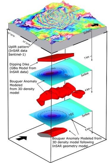

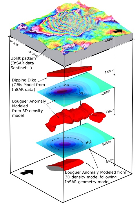
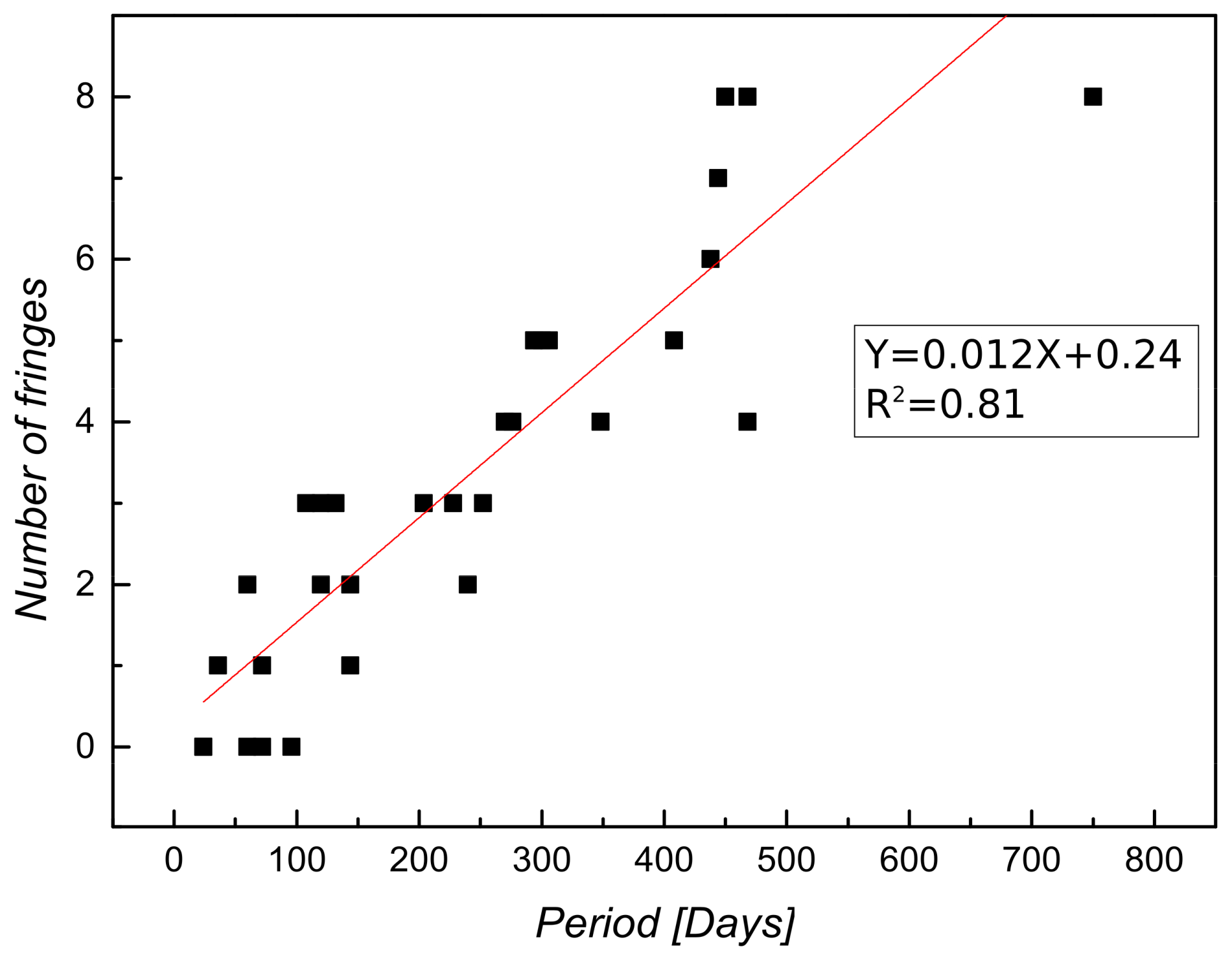
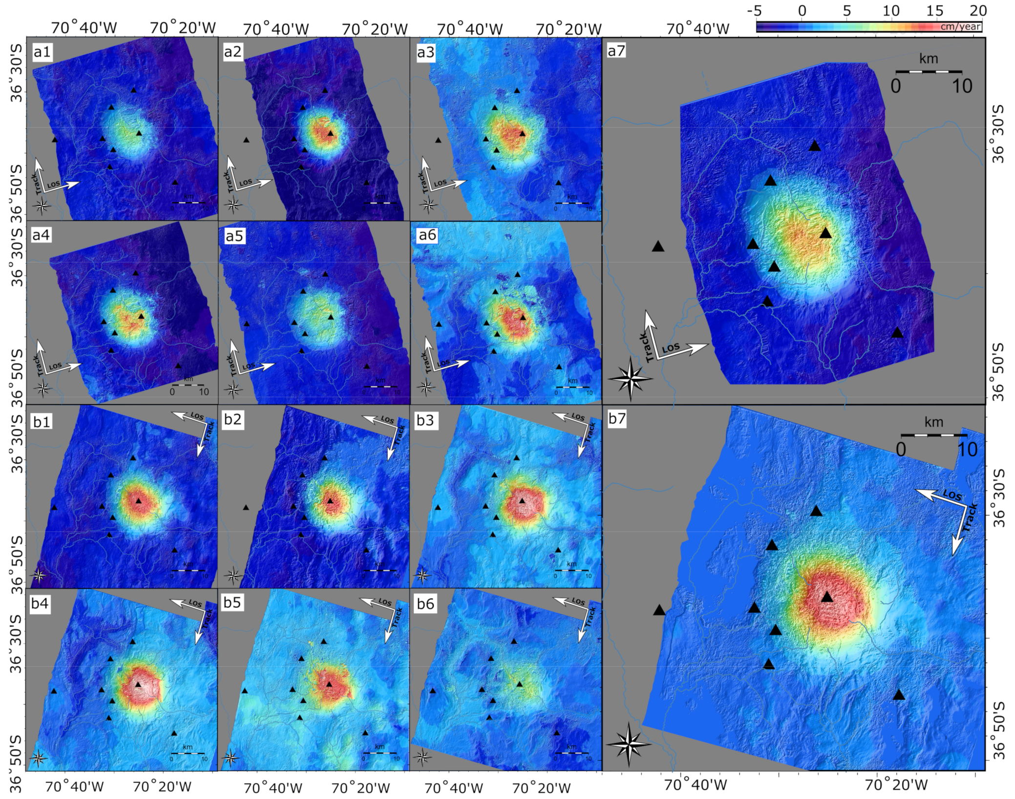
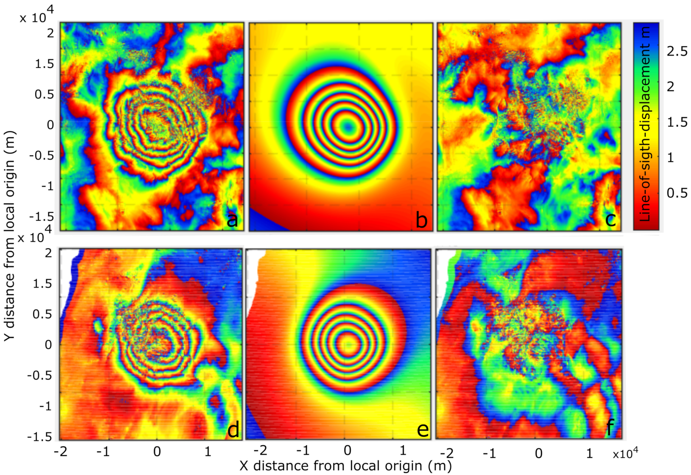
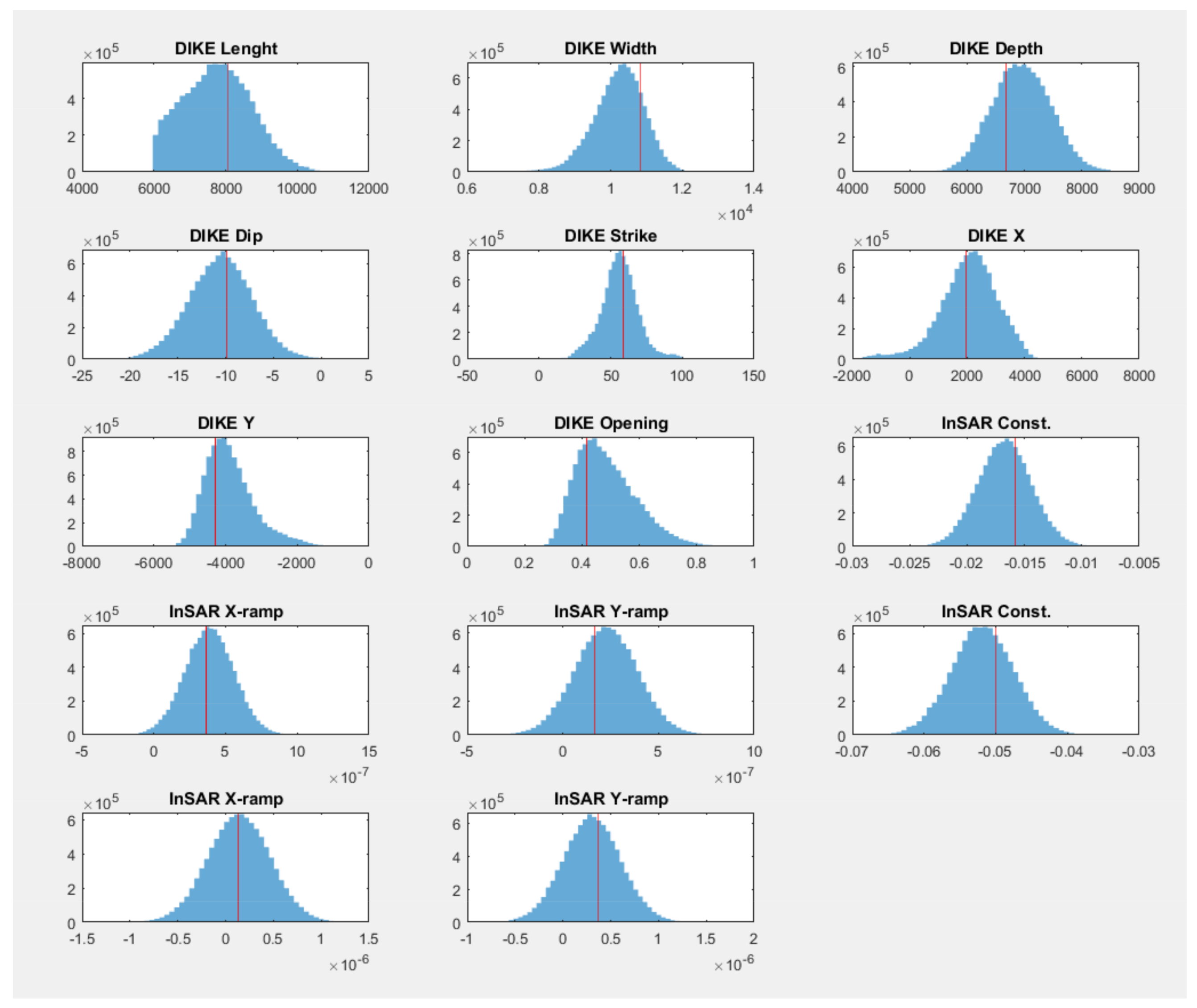
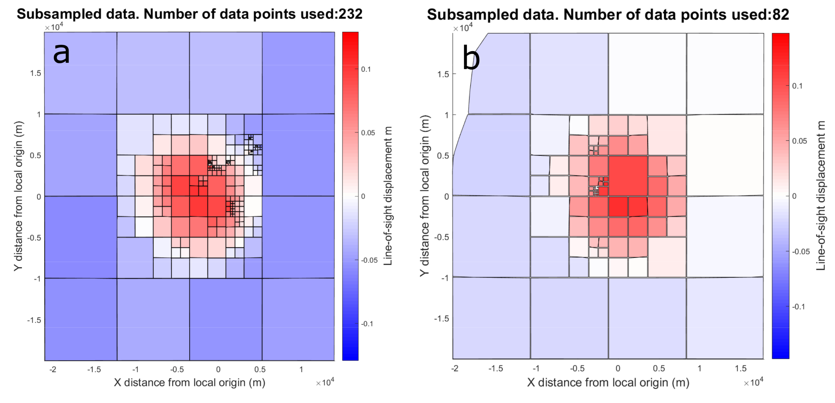
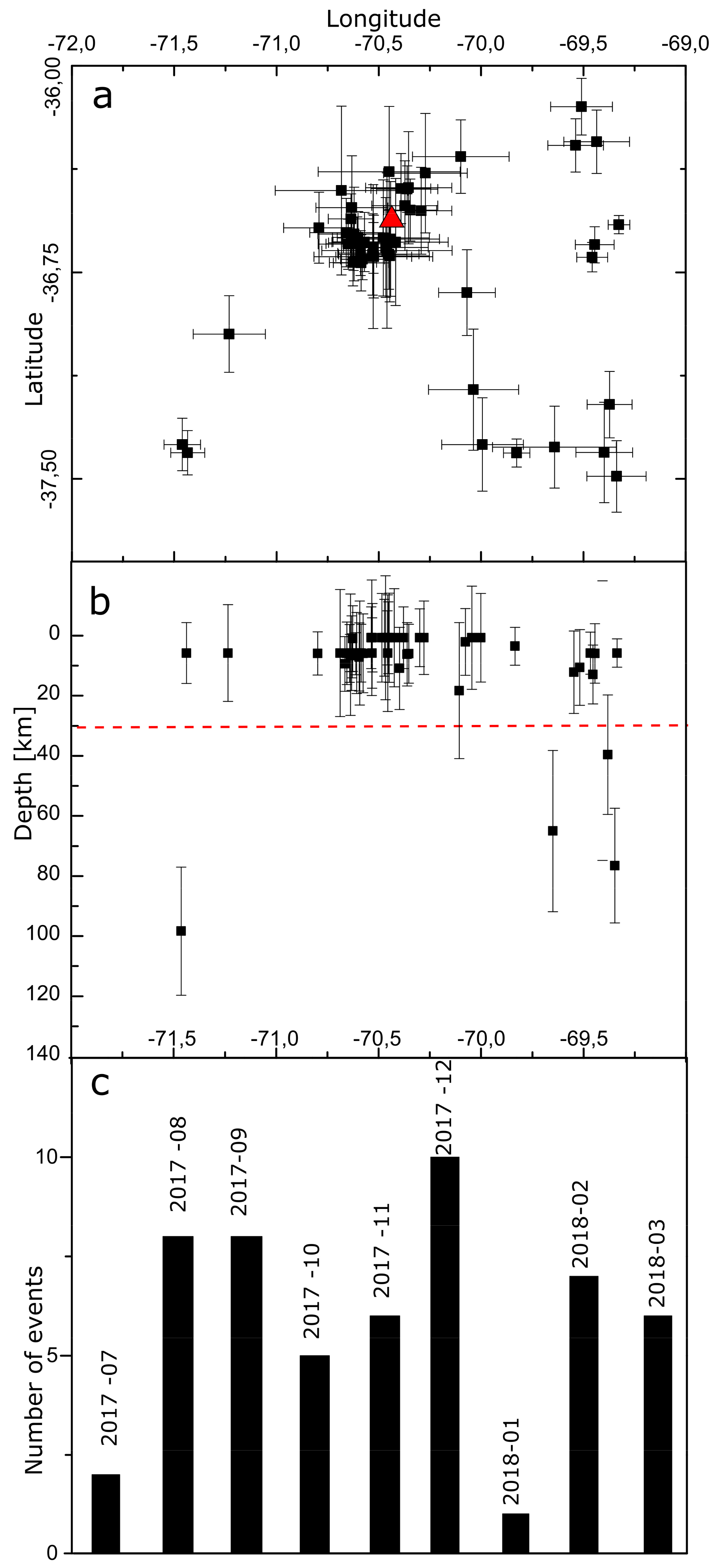
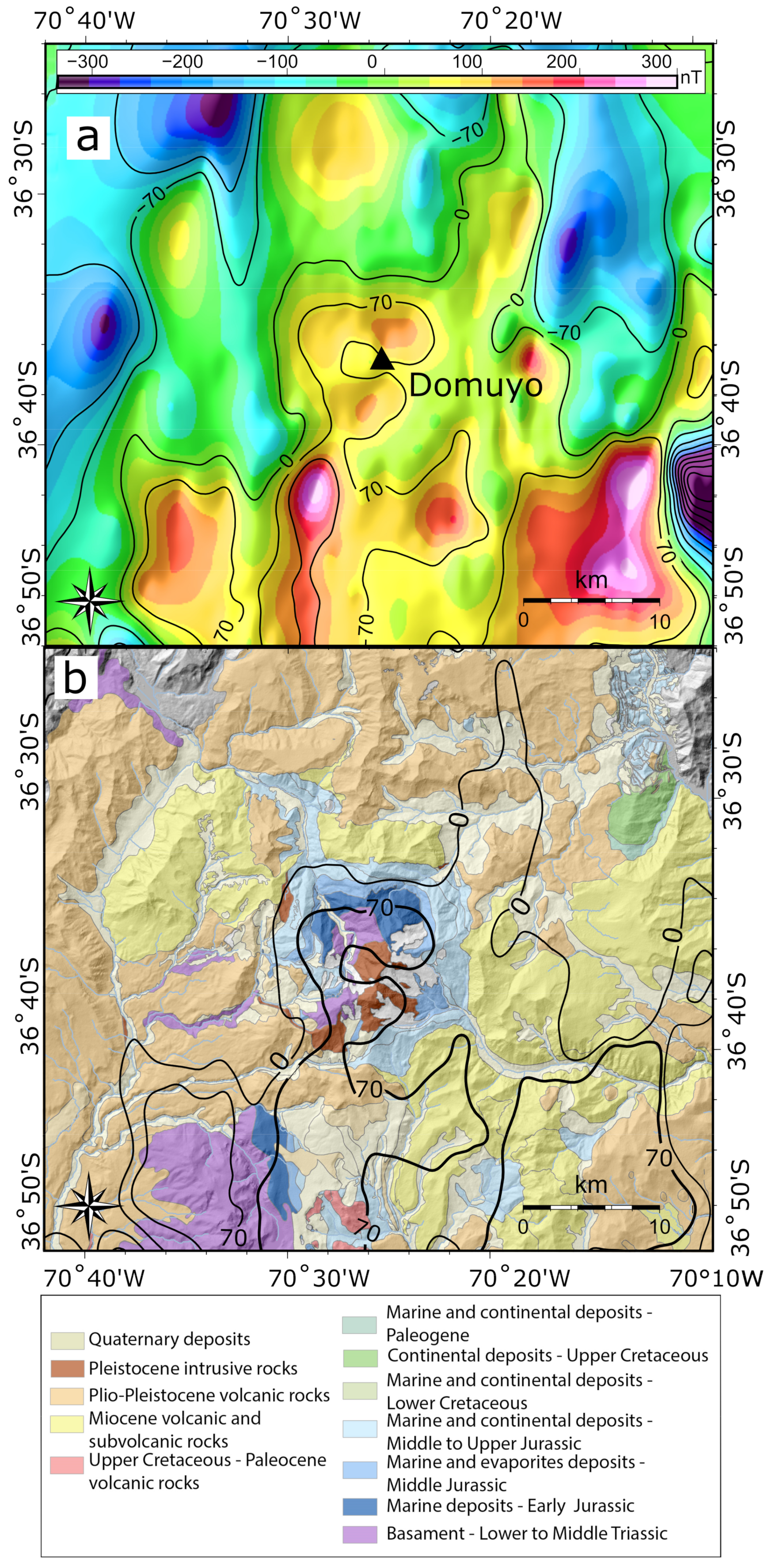


