1. Introduction
Around the world, wind energy conversion systems (WECS) are a competitive alternative to fossil fuels to generate electricity without the production of greenhouse emissions. In recent years, the installed capacity of these systems has dramatically increased, having a presence in more than 80 countries. Within this panorama, the investigations of the interaction between the electrical grid and the wind turbine (WT) installation is an important research topic since it is necessary to prevent energy loss due to disturbances in the WECS, including the reduction of power quality because of the presence of harmonic currents. In this regard, the type-4 offers a total decoupling between the WT and the electrical grid, meaning that any disturbance in the AC grid can be dealt with within the converters of the turbine without affecting the wind generator. However, the WT converter itself is a source of harmonic currents for the AC grid and it can affect the proper functioning of the network if not dealt with properly, especially in places with weak grid connections such as remote communities.
Distributed renewables energy access (DREA) offers a conventional power generation alternative to remotely located communities, without the problems produced by the fossil fuel combustion [
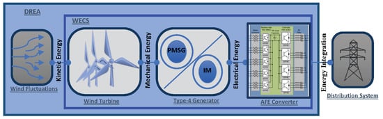
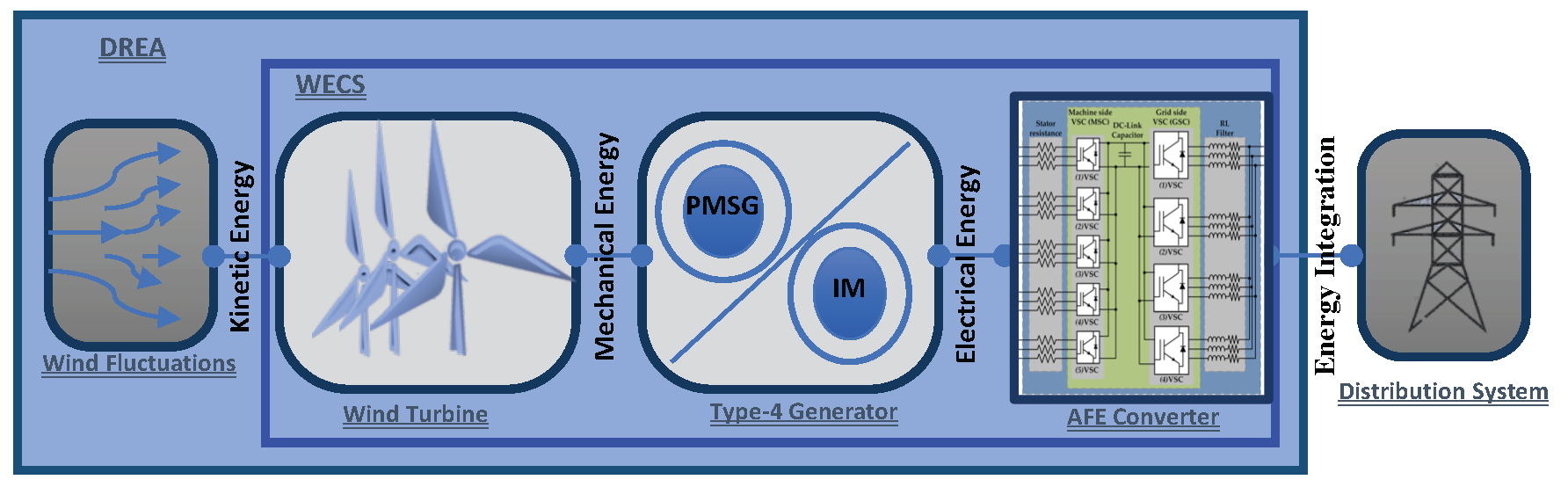
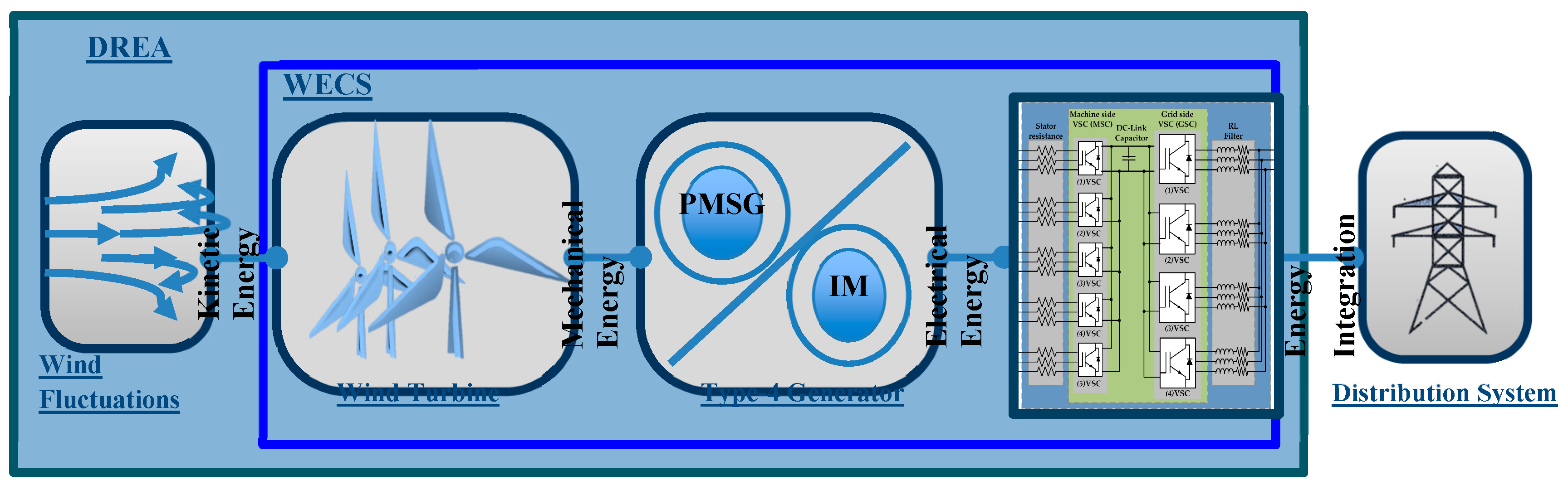
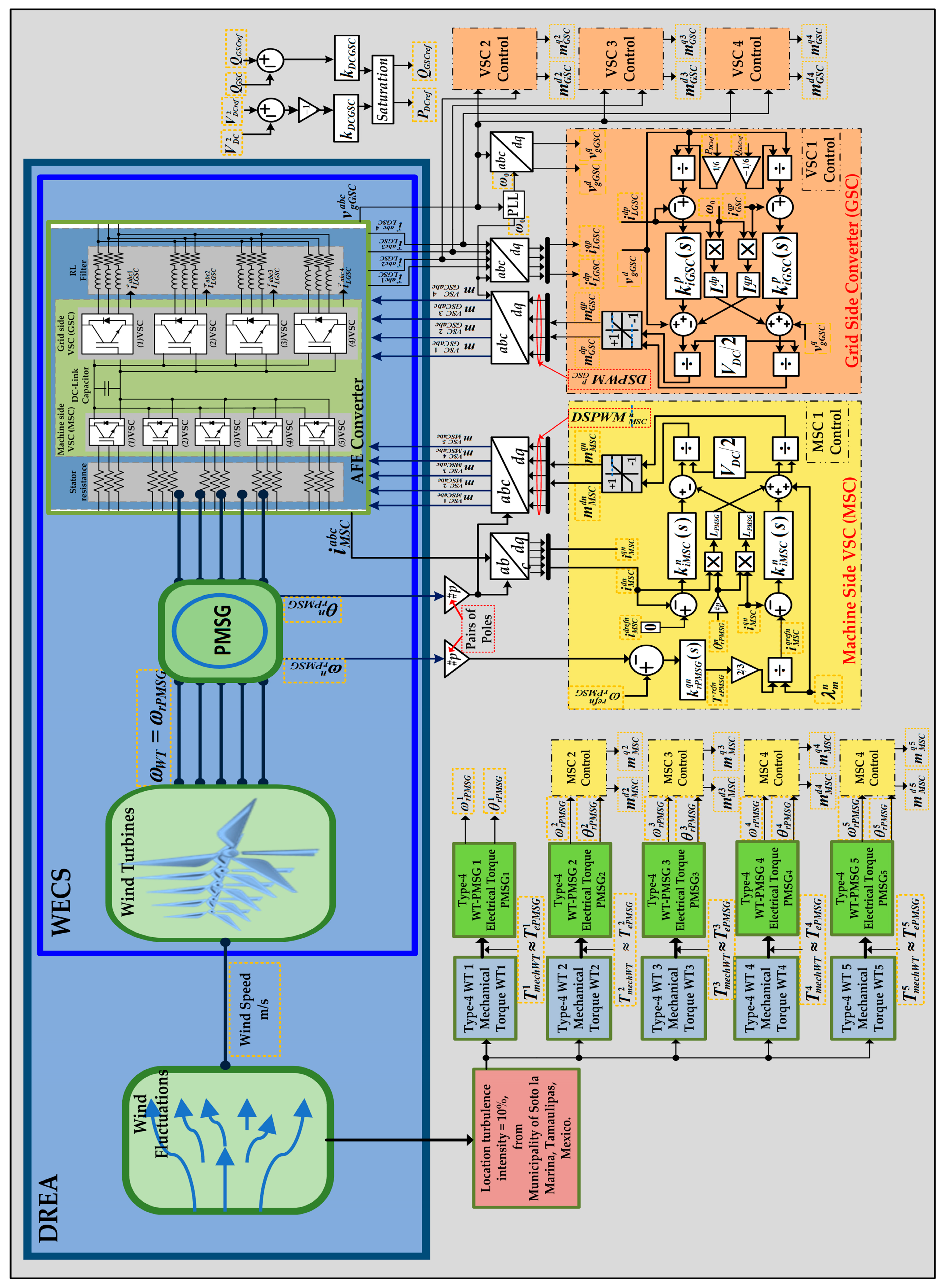
1]. One-way to generate a point of common coupling (PCC) between the DREA and AC grid is the WECS implementation,
Figure 1 shows this process. As evidence of it: by the end of 2016, a worldwide production of 487 GW is installed [
2]; in 2017, a total capacity of 539.291 GW was generated, of which China is the country with greater generation, producing 187.73 GW [
3]; and in 2021, the installed capacity is expected to exceed 800 GW [
4]. In Mexico, wind energy generation represents the second largest source of electricity production. At the end of 2016, generation of 3.527 GW was integrated; in 2017, 480 MW was added, resulting in a total generation of 4.007 GW. If this increase continues, Mexico will integrate a power capacity of 12 GW between 2020 and 2027 according to information provided by the Secretariat of Energy (SENER) [
5,
6].
WTs, generators (such as the permanent magnet synchronous generator (PMSG)), closed loop controls, and power electronics converters are included in a WECS. Therefore, in order to fully evaluate the effects of harmonics and wind fluctuation in the power grid, high order model creation is required for WECS integration, in which wind and system dynamics are reflected [
7]. In any case, the main objective for a power network is that the n-units of the WT remain connected to the AC grid under the presence of energy quality-adverse phenomena; for example, sags and swells in voltage or higher THD of current, all consequences of wind variability and the power electronic converters of the WTs. The energy from the WTs is supplied through power electronic converters such as AFE converters [
8], which are formed by the active connection of two VSCs, the front-VSC called the machine-side converter (MSC), and the end-VSC, named the grid-side converter (GSC). In addition, a WESC can improve its range of variable speed operation if designed as a type-4 WT-PMSG installation, which decouples the grid frequency from the generator frequency and the full power output of the turbine is provided to the grid by a full power electronic converter [
9].
Nowadays, multiple investigations are currently analyzing the type-4 WT-PMSG characteristics and attempting to solve the technical problems related to its installation. For example, in [
10], PMSG inertial response analysis using different virtual synchronous generators (VSG) is presented; it is observed that the frequency support capacity varies in each of the analyzed VSGs; consequently, the grid frequency is unstable. Therefore, the authors propose an optimal WECS control scheme with base power of 1.5 MVA, keeping the AC grid frequency stable regardless of any VSG connection.
In [
11], the authors proposed a unified power control strategy in a WECS–PMSG with base power of 1.5 MVA, operating under asymmetrical faults and different conditions established by grid codes. In this strategy, the MSC is used to control the DC-link voltage and the GSC is responsible for the active and power injected/absorption into the AC grid, that is, the MSC automatically reduces/increases the generator current, keeping the DC-link voltage constant while the GSC varies the AC grid current, performing power compensation. In the presence of asymmetric faults, the current distortions are mitigated. In [
12], the authors developed a fixed-pitch small-scale WECS–PMSG control with base power of 10 kW. The AC-DC-AC converter is controlled by space-vector modulation based on direct torque control (SVM-DTC). Thereby, the provided control references are followed for the flux linkage magnitude and the pair angle. Finally, in [
13] the authors propose a WECS–PMSG strategy control with base power of 2 MVA, in which the WECS grid current THD is decreased by up to two times.
In this paper, a DREA based on type-4 WTs in a distribution system is integrated. The digital controllers of the system are deployed in order to provide the following behavior for any WT operation point:
- (i)
WT-PMSG frequency regulation, for which the MSC is used.
- (ii)
PCC voltage regulation, for which the MSC is used.
- (iii)
Reactive power compensation, for which the MSC and GSC can be used.
- (iv)
The DC-link constant, for which the GSC is used.
- (v)
THD reduction up to four times, for which the GSC is used.
The DREA simulation in Matlab-Simulink® is analyzed under typical wind speed conditions for a location in a municipality of Tamaulipas, Mexico with real data from wind and grid conditions of the system. The obtained results show the DREA effectiveness and robustness through the WECS analysis, design, and modeling, producing a total transferred power capacity of 10 MVA into the AC distribution grid.
This paper is organized as follows:
Section 2 delimits the region in Mexico selected to assess the effectiveness of the controller under typical winds speed conditions.
Section 3 details the analysis, modeling, and design of the DREA integration, where the machine-side VSC modeling, DC-link control, and the grid-side VSC modeling of the AFE converter are analyzed.
Section 4 presents the DREA based on WECS characteristics.
Section 5 shows the simulated study case results, these are focused on the Location of Soto la Marina, Tamaulipas, Mexico. Finally, in
Section 5, the conclusions are presented.
2. Delimiting the Study Case
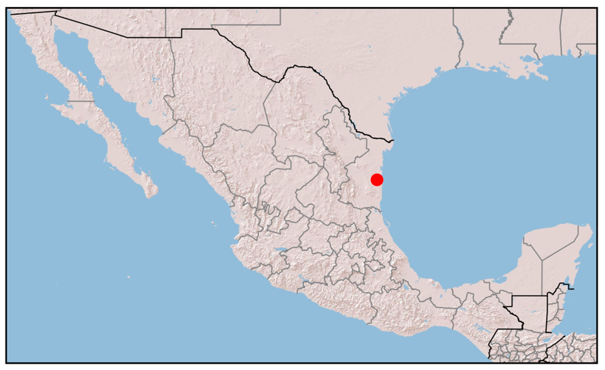
To test DREA integration through WECS, wind speed variability is obtained from a real wind speed data set. The selected location is Tamaulipas, one of the states of Mexico with prominent wind speeds suitable for wind power production; a detailed description of resource assessment is reported in the literature [
14,
15]. The municipality of Soto la Marina was selected as the study case, where an anemometric mast was installed at latitude 23° 53′ 25″ N and longitude 98° 01′ 37″ W. Ten minute mean wind speeds, standard deviations, and directions were measured and recorded from the first of January until the 31st of December for 2006 at 20 and 40 m heights.
Figure 2 illustrates the anemometric mast location.
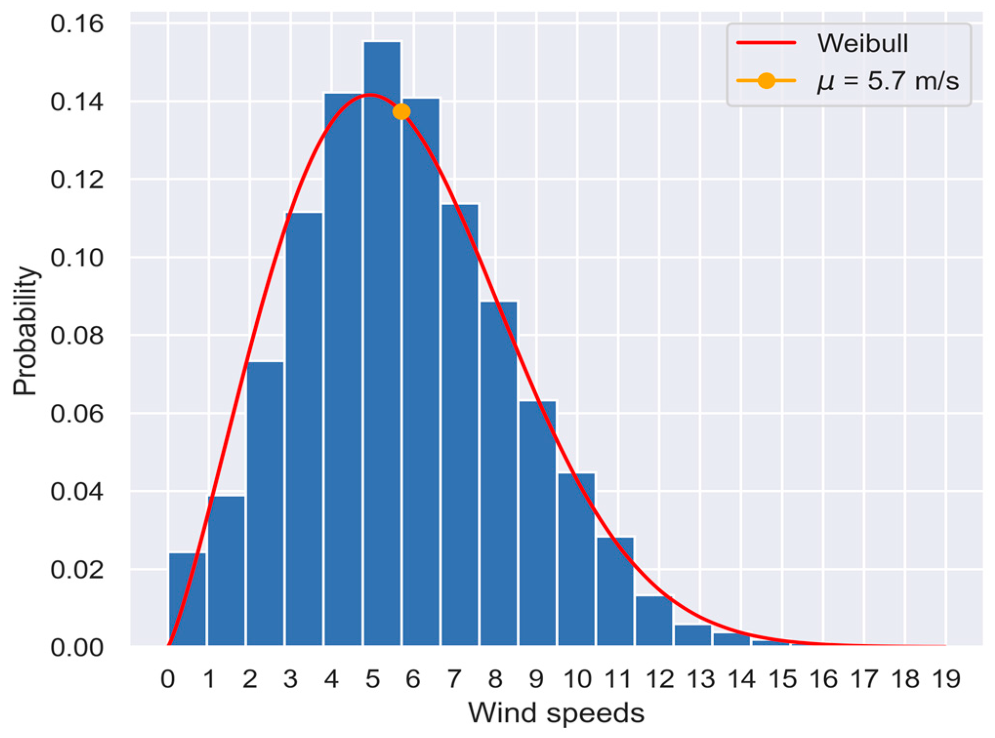
Representing a wind speed data set by a probabilistic model is a common task to study a location from a wind power perspective. The Weibull distribution function
is widely used in the literature in this regard [
16]. Equation (1) represents the mathematical expression of this probabilistic model
where
u is the wind speed and
k and
c represent the scale and shape parameters, respectively.
The histogram of the wind speed data set and the Weibull probability distribution are presented in
Figure 3. It is observed that the mean
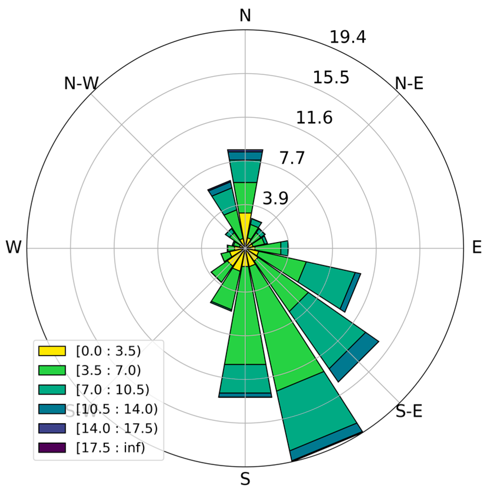
μ of the model is 5.7 m/s and the mode is between 5 and 6 m/s. These central values of the probabilistic distribution are used to define the most common wind speed in the location; therefore, the associated variability effects are used to test the converter effectiveness under this wind variability. The wind rose is presented in
Figure 4 as complementary information. It is observed that wind speed comes mainly from between the south and south-east directions.
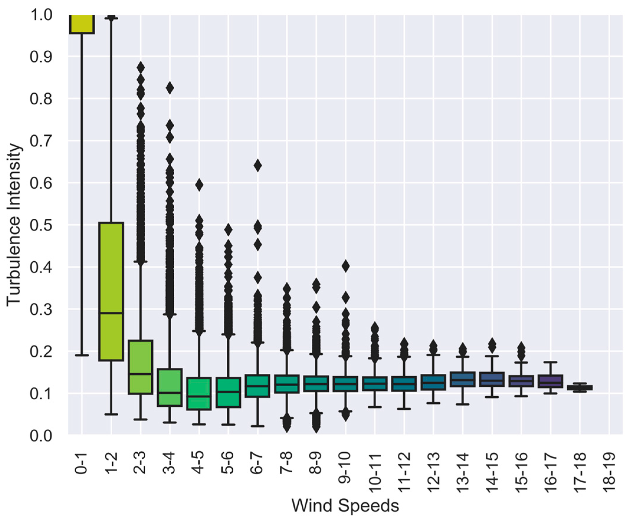
Turbulence intensity (TI) is the parameter used to analyze wind speed variability. It compares the dispersion for a set of wind speeds , where , with the mean value , for a period of time, this variability is represented by a percentage and assumes that during the studied time period, the data is normally distributed. It is computed according to Equation (2)
Turbulence intensity analysis compares the wind speed dispersion with the mean wind speed for a specific time. For a wind speed data set, it is possible that for equal mean wind speeds, different dispersion values may be measured, indicating a broad set of turbulence intensity values commonly represented by boxplots as observed in
Figure 5.
Figure 5 presents the TI values for all the recorded wind speeds. To summarize them, they were grouped by 1 m/s bins and are represented by boxplots for each group. TI mean values range between 10% and 18%. It may be noticed in
Figure 5 that the wind speeds’ dispersion is decreased as the magnitude of the wind velocity is increased, which are commonly described as stable wind speeds. To define the case of analysis in this paper, the mean TI is selected from the most common wind speeds, which is 10%. With this condition, the DREA through WECS based on the type-4 WT is tested under typical wind speed dispersion conditions for the region of Soto la Marina.
3. Analysis, Modeling, and Design of the DREA Integration into the Distribution System
This section describes the modeling, design, and analysis of a DREA interconnected to the distribution system based on WECS. Then, a WECS is required in the transformation from kinetic energy (provided by the wind circulation) to electrical energy.
As
Figure 1 illustrates, the given kinetic energy of the wind fluctuations moves five wind turbines, each with an individual capacity of 2 MVA, transferring a total power of 10 MW of equivalent power at full load. Subsequently, the generated mechanical energy by the WTs is transformed in electrical energy by means of a PMSG. Finally, an AFE converter provides the conversion of low frequency power coming from the generator into nominal frequency of the distribution system.
The AFE converter is modeled by the connection of two VSCs, where one VSC is called the MSC, through which the transferred current compensation is made by induction from the rotor to the stator, and the PMSG angular frequency regulation is carried out; while the other VSC is named the GSC, wherein the feedback current control is performed at the AC grid and the DC-link voltage constant is maintained [
17].
3.1. Angular Frequency Regulation based on MSC
Type-4 wind turbines enable a variable rotor speed operation of +/− 60% of the nominal generator angular frequency. Thanks to this, type-4 wind turbines are able to provide better maximum power tracking for variable wind speed conditions when compared with other types of wind turbines of equivalent capacity. Type-4 WTs can be constructed using induction generators (IG) or a PMSG; the difference is that the latter does not contain gearboxes, which reduces the cost of installation and maintenance [
18,
19].
The WT angular speed is defined as:
where
is the angular frequency of the PMSG. As such, the PMSG nominal power is determined by:
where
is the PMSG nominal power,
is the WT mechanical torque,
is the PMSG electrical torque and
is the WT angular speed calculated by the machine revolutions number per minute, as
.
Subsequently, the WT-PMSG variable speed control is represented using a plant model, where the dynamic characteristics are shown as a time function, as:
where
D is the viscous damping and
H is the inertia constant; these are variables of the PMSG.
By using Laplace transform, Equation (5) in the Laplace frequency domain is represented, i.e.:
Considering that in steady state it is fulfilled that
TmechWT ≈ TePMSG, then, Equation (6) is represented as:
Tracking the
ωrPMSG reference commands in the close loop transfer function, the Proportional-Integral (PI) compensators are used, the feedback loop is:
where
and
are the proportional and integral gains, respectively.
From (8), the relation between the plant pole and PI compensator zero is obtained, and the control gains are generated using the following expressions:
where
is the bandwidth of WT-PMSG closed loop control and the subscript
τPMSG is the response time of the first order transfer function. These are selected according to the WT-PMSG transferred power.
3.2. Transferred Current Compensation by MSC
The input–output transferred power between the WT-PMSG and MSC in the time-domain relationship is given by:
Next, it is represented in the
dq reference frame, generating the VSC AC-side as:
The MSC AC-side voltage in the
dq reference frame is generated with the DC-link voltage generated by the GSC:
For the analysis of MSC control in currents mode, the plant model is generated, which is based on the modulation index vector
. That is:
where
is a compensation vector with additional signal control.
By substituting (15) and (16) into (14), and the result is substituted into (12) and (13), respectively, a first order linear system is obtained; that is, Equation (17) describes the MSC AC-side plant model.
In the MSC AC-side, the electrical torque control uses (17), for which, the generation of two decoupled, first-order, linear systems in the frequency domain is necessary, i.e.:
Following the
reference commands in the closed loop,
is replaced by the PI compensators, that is:
where
and
are the proportional and integral gains, respectively.
The generated pole in (17) is , which is close to the origin. As a consequence, the magnitude and the phase of the loop gain start to drop from a relatively low frequency. In this context, the new zero selection through the PI compensator can avoid this behavior. To do this, the plant pole is eliminated by a zero of the PI compensator, with .
The relation between the plant pole and PI zero is obtained as:
where the
response time is ten times smaller that
in the MSC feedback current control.
Successively, the transferred power from WT-PMSG through the electric torque is calculated considering that the WT-PMSG rotor has a cylindrical geometry, and this means that
, generating a closed loop control based on
, i.e.,:
3.3. DC-Link Voltage Control Through GSC
The VSC correct operation requires that DSPWM signal switching frequency to be ten times higher than the AC grid frequency and that the DC-link voltage is at least 1.1 times greater than the line to line voltage on the AC grid, as:
Then, through the averaged model of the VSC, the feedback DC-link control is performed, as long as the modulation index (
) is defined as a sinusoidal variable in the continuous set [−1, 1]. The above represents the average relation between the VSC voltage and current in a switching cycle, i.e.:
The DC-side relation of the GSC is established by:
The transferred power by the GSC is obtained from the DC-link, as:
Knowing that the active power is the capacity to perform work in a given time, the stored capacitor energy is defined by the integral area under the curve:
In order to maintain the DC-link regulation, it is necessary the GSC plant is in voltage mode control. Replacing Equation (28) in (27) and applying the result in (26), Equation (29) in the time domain is generated:
The plant is determined by (28) in the Laplace frequency domain.
The
reference commands the PI compensators in the close loop, producing:
where
and are the proportional and integral gains, respectively.
The generated pole in (31) is , which is close to the origin. As a consequence, the magnitude and the phase of the loop gain start to drop from a relatively low frequency. In this context, the selection of a new pole through the PI compensator can avoid this behavior. To do this, the plant pole is eliminated by a zero of the PI compensator, with .
The relation between the plant pole and the PI zero is obtained as:
where the subscript
is the response time in the first order transfer function of the GSC in voltage control mode.
3.4. Feedback Current Control by GSC
The VSC input–output power transfers between delivering voltage node
and the receiving voltage node
along
can be analyzed through the time-domain relationship of the VSC AC-side in the GSC, given by:
Subsequently, Equation (34) is represented using the
dq reference frame by equivalent equations based on the Clarke and Park transformation. Then, the
dq model derived from the VSC AC-side is described as:
where the presence of
indicates the coupled dynamics between
and
.
Based on Equation (24), in the
dq reference frame is generated:
Starting with Equation (37), the modulation index vector
is changed, where the aim is plant model generation, in which the GSC with current mode control is represented. That is:
where
is a vector of additional control inputs.
By substituting (38) and (39) into (37), and substituting the result into (35) and (36), respectively, a first order linear system is obtained; that is, Equation (40) describes the GSC AC-side plant model.
In the GSC AC-side, active and reactive power control is performed using (40), for which the generation of two decoupled, first-order, linear systems in the frequency domain is necessary, i.e.:
With the purpose of racking the
reference commands in the close loop, the PI compensators are used, producing:
where
and
are the proportional and integral gains, respectively.
The generated pole in (42) is , which is close to the origin. As a consequence, the magnitude and the phase of the loop gain start to drop from a relatively low frequency. In this context, the new zero selection through the PI compensator can prevent this behavior. To do this, the plant pole is eliminated by the PI compensator zero, where .
The relation between the plant pole and the PI zero is obtained as:
where the subscript
is the response time in the first order transfer function of the GSC feedback current control. This is selected to be ten times smaller that
based on the final transferred GSC current.
Subsequently, the active and reactive powers are independently calculated through the current vectors in (45) and (46), respectively.
The
and
elements values are obtained using the total values of
and
, such as:
where
is the GSC output power,
is the line to line voltage on the GSC AC-side, and
is the current that flows through the corresponding PCC where the GSC is connected.
The base GSC system impedance is . The value of is selected as 15% of the base GSC system impedance, that is: ; subsequently, and , where ω0 is the system nominal frequency. The and values vary according to the application, in a range from 0.1 Ω to 0.5 Ω.
5. Simulation Results
The case study shown in
Figure 6 verifies the correct DREA operation. For example, in
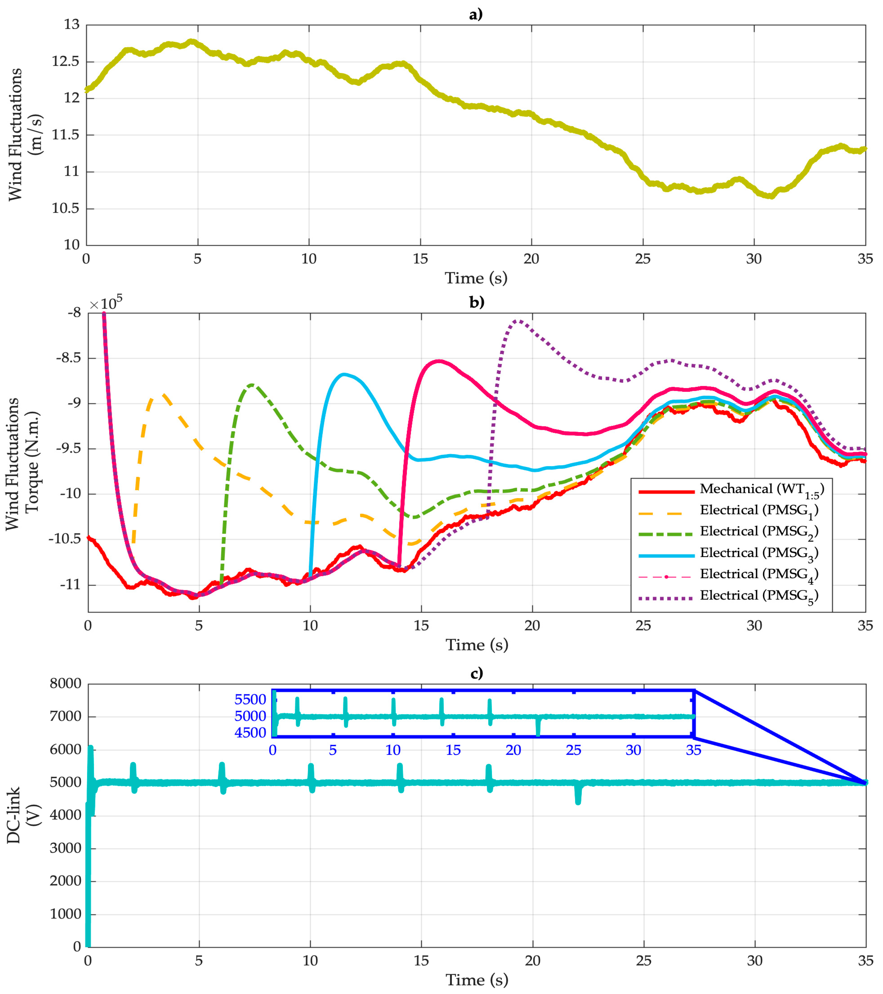
Figure 7, the main parameters’ behaviors at the WECS are shown.
Figure 7a shows the wind fluctuations speed applied to the WT-PMSG. These are generated in Matlab-Simulink
® by RISOE National Laboratory based on Kaimal spectra.
Figure 7b shows the five mechanical torques (red line) and the five electrical torques (yellow, green, blue, pink, and purple lines). In the DREA, the mechanical torques of the five WTs (that make up the WECS) work according to the generated wind fluctuations model in
Figure 7a, but the angular velocity control,
, in each WT-PMSG is made at different times. That is, the WT-PMSG1 control begins at the time of 2 s, the WT-PMSG2 control starts at 6 s, the WT-PMSG3 control starts at 10 s, the WT-PMSG4 control starts at 14 s, and the WT-PMSG5 control starts 18 s. This means that the mechanical torques are followed by the corresponding electric torque in the specified time of each WT due to the robustness of the closed loop control in
. In addition, once the transient has passed,
Figure 7c shows that the DC-link is re-established and remains constant in the presence of the initial operation of each WT. This is due to the robustness of the GSC feedback control, through which the DC-link remains constant. Finally, DC-link restoration is observed at t = 22 s due to the reactive power injection by the GSC in the distribution grid.
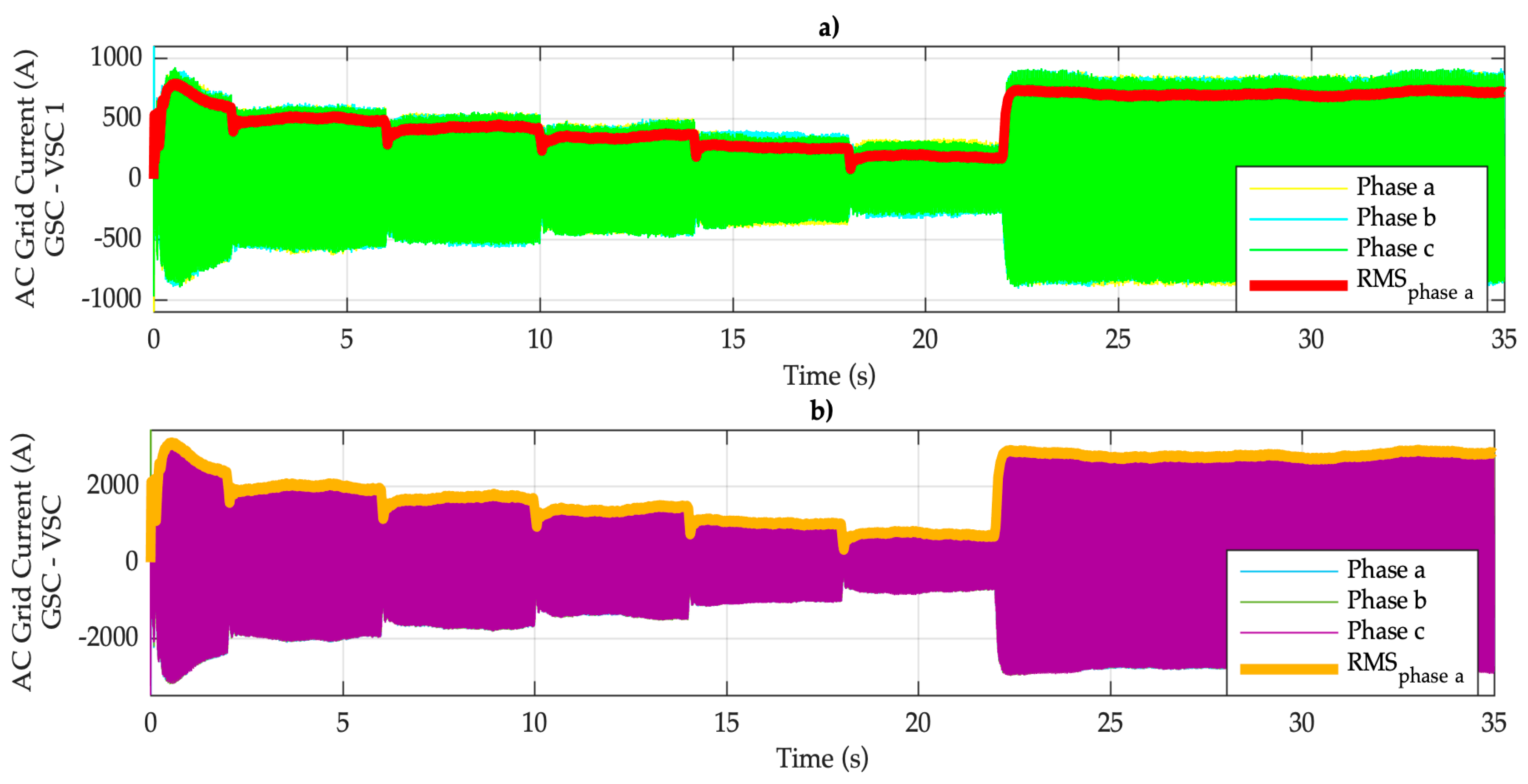
Figure 8 shows the GSC current injection/absorption in the distribution grid, which is formed by four-VSCs connected in parallel.
Figure 8a shows the handled current portion in the VSC 1, and its RMS current value is represented by the red line. It is worth mentioning that VSC
2, VSC
3, and VSC
4 transfer the same quantity of current.
Figure 8b shows the total current handled by the GSC.
Figure 8 also shows the current transients according to each integrated WT-PMSG. In addition, at t = 22 s, the current response due to the reactive power injection of 10 MVA in the distribution grid is observed, reestablishing and keeping the DC-link voltage constant (as shown in
Figure 7c) in the presence of this power injection due to the robustness of the proposed control law.
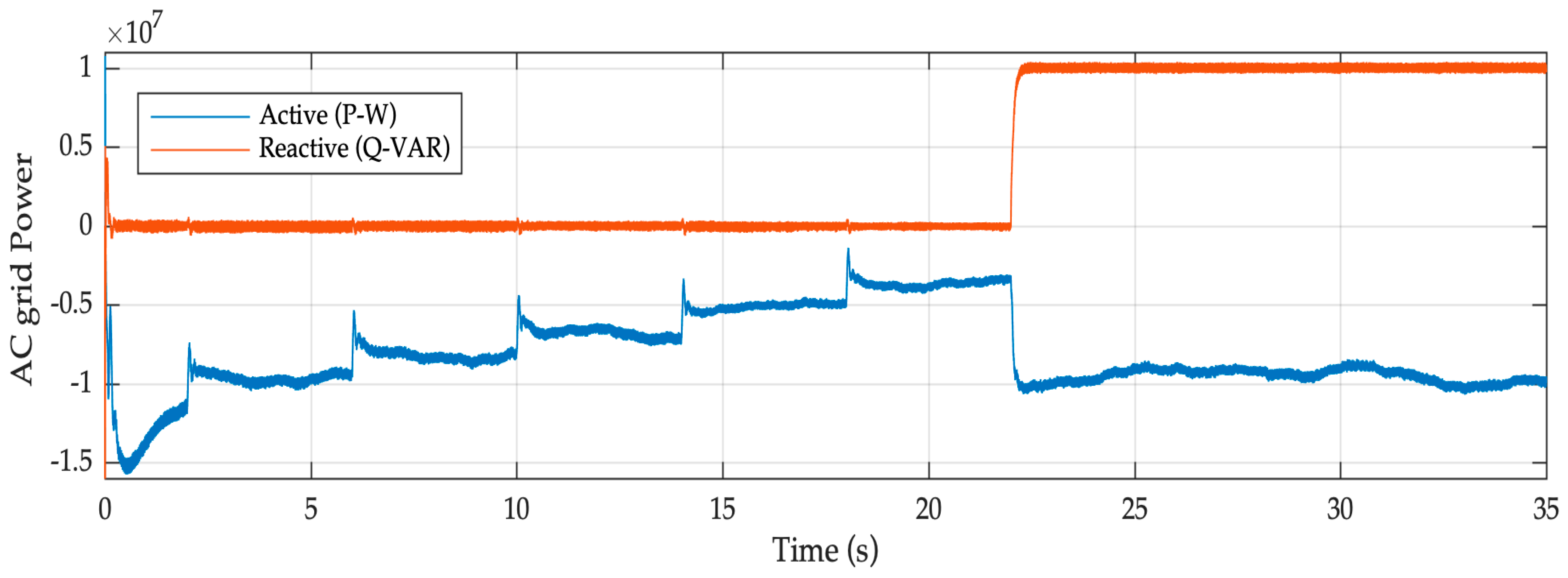
Figure 9 contains the generated active and reactive power in the DREA in which it is observed that the generated active power at the WT-PMSG is negative because it is measured from the distribution grid, meaning that it is the active power injected into the AC grid. Specifically, active power steps are generated due to the consecutive start of the WT-PMSGs every 4 s, starting at t = 2 s with WT-PMSG1 and ending at t = 18 s with WT-PMSG5, as seen in
Figure 7b. In addition, once the five turbines are activated, the proposed control efficiency is tested by an additional reactive power injection of 10 MVA at t = 22 s because the AFE converter is able to inject current without disturbance, as seen in
Figure 8b. The above is possible because the AFE converter is designed with a power capacity of 10 MVA.
To achieve current THD reduction, it is necessary to individually analyze and calculate the harmonic content in each VSC connected in parallel [
20]. A DSPWM modulation signal with different phase shift is used in each three-phase VSC; that is, the carrier signal angle of each VSC is modified, while the modulation signal’s angle remains constant [
2,
21]. Subsequently, the current output signals of each VSC (
Figure 8a) are added, generating the total GSC current (
Figure 8b).
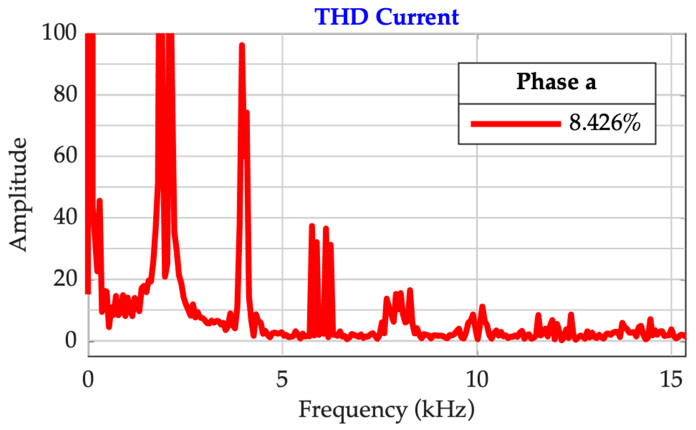
Figure 10 shows the current THD in the total GSC current without phase shift angle in the DSPWM switching signals, which corresponds to 8.426%. This happens because the generated harmonics between the VSC and WT-PMSG are not constant; they vary according to the switching frequency and the proposed control law applied to the AFE converter.
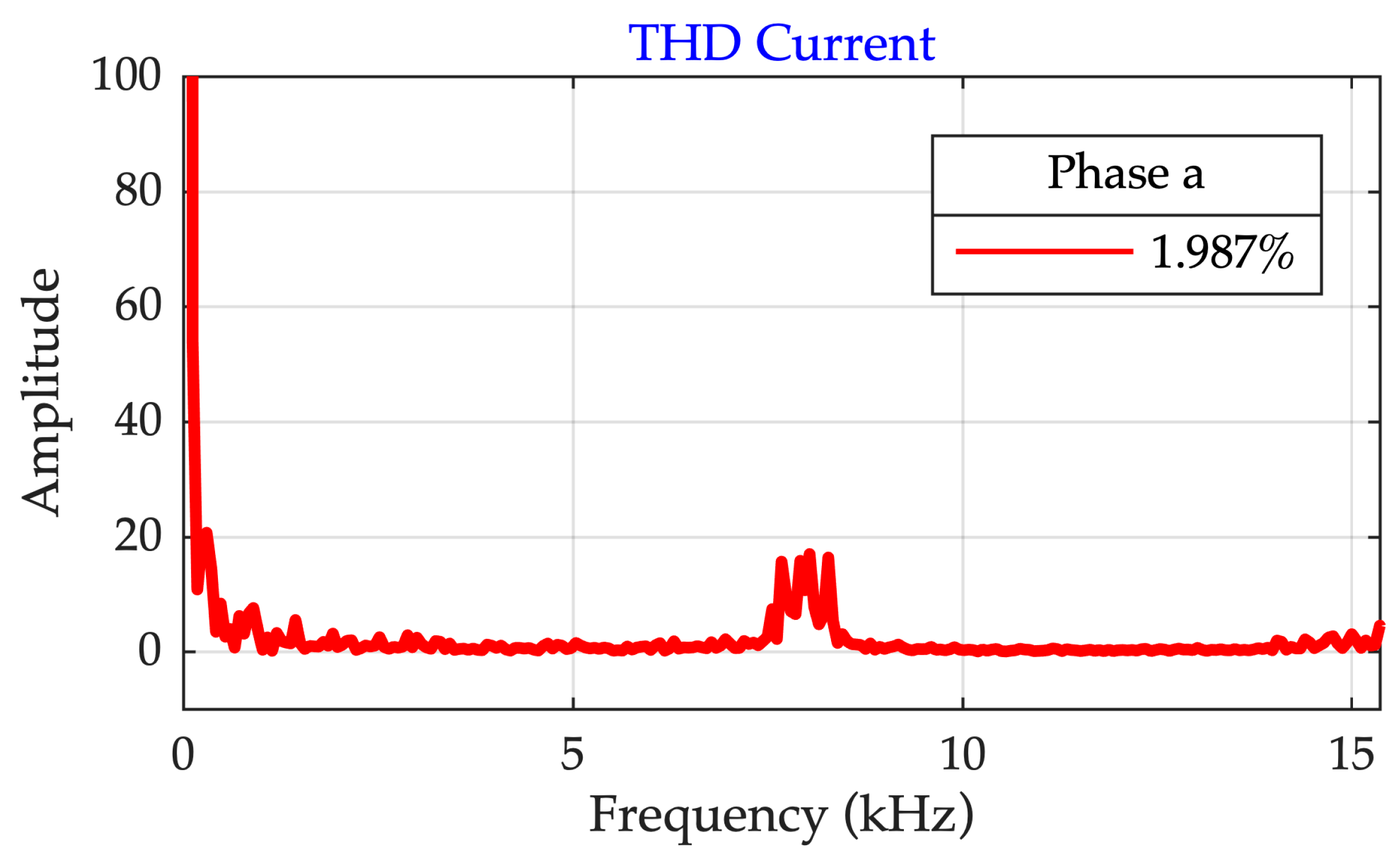
Finally,
Figure 11 shows the current THD in the total GSC current of
Figure 8b with a phase shift angle in the DSPWM switching signal equivalent to 90°. This is applied between the carriers of each VSC connected in parallel, generating THD reduction up to 1.987%.
6. Discussion
In this paper, the design, analysis, and simulation of a DREA based on WECS formed by five type-4 WT-PMSGs with individual nominal power of 2 MW under typical real wind speed conditions are presented. The first stage of analysis is presented by a description of wind speed and directions of the anemometric mast located at Soto La Marina, Tamaulipas Mexico. A Weibull probabilistic model represents wind speeds, and wind speeds between 5 and 6 m/s were the most probable, meaning the estimated TI was approximately 10%. These typical dispersion conditions were used to feed the model.
The main contribution is the integration of five WT-PMSGs into the distribution system by means of an AFE converter, in which the AFE converter is formed by the parallel connection of four power VSCs of 3 MW each.
Through this topology, the following advantages were achieved:
Improved performance of the WECS due to integration of type-4 WT-PMSGs, which have no gearboxes.
Formation of the GSC through the parallel connection of four VSCs, making each VSC transfer only a portion of the total power.
Mitigation of the current THD by up to four times, due to the incorporated phase shift angle equivalent to 90° in the DSPWM switching signals.
Transfer of power equivalent to 10 MVA generated by the DREA into the AC distribution grid.
It is worth mentioning that this region in Mexico is selected because it has optimal wind speeds and turbulence conditions for type-4 WT-PMSGs to work properly. Using the wind characteristics and specific types of wind turbines, the control law of the AFE converter was determined, designed, modeled, and simulated, thus fulfilling the goal of the manuscript; a four-fold reduction in current THD in the DREA integration into the AC distribution grid.
7. Conclusions
In this paper, we achieved THD reduction in the integration of a DREA through WECS under the wind speed conditions presented in Tamaulipas, Mexico. The WECS consisted of the connection of five type-4 WT-PMSGs, each with an individual capacity of 2 MVA.
The GSC converter was formed by four VSCs connected in parallel, generating an AFE converter with an individual capacity of 3 MVA. The AFE converter was used for current THD reduction and it was controlled by a different DSPWM switching signal, in which a phase shift angle equivalent to 90° was applied between the carriers of each VSC connected in parallel, generating up to four-fold THD reduction.
The results of this proposal have been supported by a complete mathematical model and the simulations in Matlab-Simulink® demonstrate the effectiveness and robustness of the methodology, mitigating the THD from 8.426% to 1.987% and transferring a total wind power capacity of 10 MVA to the AC distribution grid in the municipality of Soto la Marina in the state of Tamaulipas, Mexico.
This study forms the base of a methodology for the analysis of the integration of wind farms and may lead to innovative proposals under different wind farm scenarios.

 ,
, 


