Feature Selection for Blood Glucose Level Prediction in Type 1 Diabetes Mellitus by Using the Sequential Input Selection Algorithm (SISAL)

Abstract

Feature selection is a primary exercise to tackle any forecasting task. Machine learning algorithms used to predict any variable can improve their performance by lessening their computational effort with a proper dataset. Anticipating future glycemia in type 1 diabetes mellitus (DM1) patients provides a baseline in its management, and in this task, we need to carefully select data, especially now, when novel wearable devices offer more and more information. In this paper, a complete characterization of 25 diabetic people has been carried out, registering innovative variables like sleep, schedule, or heart rate in addition to other well-known ones like insulin, meal, and exercise. With this ground-breaking data compilation, we present a study of these features using the Sequential Input Selection Algorithm (SISAL), which is specially prepared for time series data. The results rank features according to their importance, regarding their relevance in blood glucose level prediction as well as indicating the most influential past values to be taken into account and distinguishing features with person-dependent behavior from others with a common performance in any patient. These ideas can be used as strategies to select data for predicting glycemia depending on the availability of computational power, required speed, or required accuracy. In conclusion, this paper tries to analyze if there exists symmetry among the different features that can affect blood glucose levels, that is, if their behavior is symmetric in terms of influence in glycemia.

1. Introduction

Diabetes is a disease characterized by high blood sugar levels as a consequence of the body’s inability to produce and/or use insulin. In a healthy human, glucose homeostasis represents a closed-loop system which is able to regulate blood glucose levels. In this way, the pancreas presents β cells which are sensitive to high glucose levels and produce insulin, a strong hormone able to reduce hyperglycemia in blood by allowing a “passage” for glucose to enter the cells.

This regulation is not naturally possible in type 1 diabetes mellitus (DM1). Patients with a certain evolution of DM1 do not produce any insulin and must inject this hormone or wear an insulin pump in order to reduce their glucose levels. Furthermore, diabetic people need to check their glucose level several times per day and, based on these data as well as other factors like meals, exercise, and many others, try to predict the evolution of their glycemia. Then, they have to decide how much insulin is required to keep their blood glucose level within a normal range (avoiding both hyper- and hypoglycemia). In this way, insulin can be delivered either by multiple daily injections or by continuous infusion using a pump which permeates under the skin.

In this context, new technological possibilities offer a new horizon in providing information in order to forecast future blood glucose levels of DM1 patients. At present, it is not possible to think about an approach to an artificial pancreas without considering continuous glucose monitoring (CGM) devices. These types of gadgets have driven a revolution in diabetes care since they provide the magnitude, tendency, frequency, and duration of fluctuations of glucose levels. Compared with conventional glucose monitoring (capillary blood glucose monitoring by using test strips), which generally provides from three to ten measures of glucose per day, CGM can deliver up to one measure per minute (1440 data per day). This is a sample frequency which should be enough for the input of a glucose control system.

On the other hand, besides CGM devices, some other gadgets in the field of biometrics can now maintain 24-h monitoring of the patient, recording important information about a person’s health. In this sense, many variables such as exercise, heart rate, hours of sleep, and so on can be provided continuously. Therefore, a combination of the information provided by both type of devices (CGM and biometric) points to the possibility of developing new ways of managing diabetes by obtaining new blood glucose prediction algorithms.

In addition to these ideas, it should be noted that recent studies in the field of mathematics, especially those related to improved ways of solving equations [1], boost the possibilities of applying new approaches to solve some remarkable challenges. Furthermore, advances in materials, electronics, electromagnetic functionalities, and many others lead to extraordinary properties in terms of field configurations [2].

Regarding this issue, to the best of the authors’ knowledge, unfortunately there is no previous work among the scientific literature with comprehensive data acquisition, since some previously published studies consider only partial monitoring, collecting only some of the features that can be recorded, or simply focus on a limited number of patients and/or data collection during a few days. On the other hand, the mentioned prediction algorithms require a previous step: a well-chosen set of variables (some of them previously mentioned: amount of insulin, meals, exercise, etc.) which need to be carefully selected and handled in order to avoid overstraining of the forecasting system. In this sense, since a proper comprehensive feature collection for blood glucose prediction has not been published, there is also no published study of feature selection which would allow the relevant past values of each variable to be chosen.

In this sense, this paper’s contribution is twofold: firstly, a good dataset has been achieved by performing a complete and continuous monitoring of different features in 25 DM1 people during 14 days and, after that, the estimation of a proper set of features has been carried out by choosing the most relevant variables along with the number of historic influential values. This way, the present work tries to analyze if there exists symmetry among the different features that can affect blood glucose levels, that is, if their behavior is symmetric in terms of influence in glycemia. Furthermore, we will study if, in turn, some features behave symmetrically between different patients (in the same way, sense, and magnitude) or if, on the other hand, some other features behave asymmetrically. This study has been performed by applying a feature selection technique called the Sequential Input Selection Algorithm (SISAL).

2. The Appearance of New Variables Due to New Devices

As previously mentioned, good prediction of incoming blood glucose levels can undoubtedly help people with DM1 to maintain good control of glycemia. In this sense, several attempts have been made previously, and the scientific literature presents a wide range of approaches to this topic. Well-known techniques like the Autoregressive Exogenous Model (ARX) [3], Interval Model Identification [4], Support Vector Machine (SVM), Artificial Neural Networks (ANNs) [5], and others can be found in a brief review. However, the sets of features used and found in the scientific literature to predict glycemia generally suffer from a lack of completeness, usually taking into account just glycemia and its historical data or, in the best-case scenario, the addition of insulin boluses and estimation of the carbohydrate intake. Moreover, it should be noted that the scarcity of patients and/or monitoring time makes the extraction of general results difficult.

However, blood glucose information has been dramatically improved thanks to CGM devices. These types of devices have been increasingly included in diabetes treatment over the last few years and their utility is undoubted in the improvement of glycemia control, as many studies have shown [6,7]. On the other hand, glycemia change is, unfortunately, a complex process and cannot be totally described solely with the previously mentioned variables. Physical activity, quality of rest, emotions, and lifestyle can intuitively help to define the process but, unfortunately, have not always been included in the glycemia-prediction problem. In fact, some of these features have an undisputed role in glucose metabolism. Exercise and physical work can lead to a rise of insulin sensitivity [8], and although they have been included as a variable in some experiments, they have been considered in an imprecise and subjective way, relying on their quantification according to the patient’s perception [9]. Heart rate has also been demonstrated to be an important feature to be included, as shown in Reference [10], where its ability to anticipate hypoglycemia was analyzed. In the same sense, skin temperature and skin conductance were studied as early as 1986 as a way to predict low sugar blood levels [11]. In addition, the quality of sleep and its duration have also been studied as relevant factors in diabetes control [12].

In any case, it has been difficult, up to now, to have a good record of the previously described data. In fact, some of the mentioned published works have been developed under specific experimental conditions and sometimes within medically controlled environments. The absence of the abovementioned variables in a predictor model has been due to difficulties in continuously registering these features but, nowadays, in addition to CGM devices, many new electronic gadgets related to health and sports are offered on the technological market. These new tools inform users, in an attractive way, about the intensity of their physical exercise, the quality of their sleep, and their heart rate at every single moment of the day. These novel resources usually adopt the shape of a smart band and, due to their sufficient accuracy, open new routes to complete a full characterization of the status of the patient and therefore to achieve better management of diabetes. The possibilities of these advanced tools have been recently reported in References [13,14]. In another recent work [15], an analysis of their advantages and disadvantages has been carried out, identifying some gaps in order to improve their usability.

Other effects which have an impact on glycemia, such as circadian rhythms and the importance of having a schedule and a routine, are well known [16] but have not yet been included in a blood glucose prediction algorithm. Finally, it can be important to take into account the influence of sex, age, and other inherent details on blood glucose levels [17,18]. However, they have also not been included in a set of features so far.

With these ideas, it seems to be useful if we know which are the most influential features, in order to lighten the computational burden of some predictive algorithms or increase accuracy if necessary. The results of this work will shed light on identifying the essential features while at the same time relegating others to a secondary role so that they can be pushed aside under some conditions. With a proper ranking of features, high demanding tasks like diagnostics, measurements, imaging, and some others, could be better addressed.

3. Background Regarding Sets of Features for Blood Glucose Prediction

How to predict glycemia is linked directly with how to arrange a relevant set of features. If we look through the scientific literature, the feature sets used are as diverse as the prediction approaches are. The simplest dataset uses only past values of glycemia to predict future ones. In this sense, autoregressive (AR) models are focused on using only blood glucose levels as a simple variable. By using an AR model, hypoglycemia can be anticipated by 30 min, as can be seen in Reference [19], with a root median squared error (RMSE) of 17.83 mg/dL. In this work, only one variable was used (glycemia), as stated in the AR model. The authors used data from 28 DM1 people but collected data for only 48 h.

Plis et al. [20] monitored glycemia only in five diabetic people for four days in 2014 and forecasted glycemia using the autoregressive integrated moving average (ARIMA) with predictive horizons (PHs) of 30 and 60 min, obtaining RMSE values of 22.9 and 42.2 mg/dL, respectively.

Regarding the use of glycemia only, we can also find the work of Pérez-Gandía et al. [21], this time using an ANN, which obtained a 45-min prediction including just glycemia data in a neural network with an acceptable error level. This method requires many data in order to calculate the vast number of weights. This takes a lot of training time and computational effort, and using only glycemia, the risk of overfitting is clear.

At this point, the inclusion of more features rises the possibilities. In Reference [22], an ARX model is applied, using only glycemia and fast insulin doses. It is able to predict PH in 45 min and uses normalized least mean squares (NLMS) to set a gain parameter, reaching 98.63% concordance in zone A of the Clarke error grid [23]. Notwithstanding, the considered patients were measured in a hospital and within an excessively controlled environment so it is not clear whether the results could be extrapolated to a daily routine. It is necessary to specify that it is common in the scientific literature not to take into account the basal insulin dosages (long-acting insulin with 24-h coverage), since they are supposed to be adjusted so that blood glucose levels are maintained within a normoglycemic steady state, assuming the absence of external disruptions. Novel basal insulins are able to cover undoubtedly 24 h and offer improved stability [24].

The inclusion of these two features (glycemia and fast insulin doses) is extended in previous works, such as Reference [25], where the previous glycemic data and insulin dosages are used to forecast future glucose levels through proportional integral derivative (PID) controllers. In this case, insulin is treated as insulin on board (IOB). This is an accumulated variable which allows one to take into account the remaining still active doses of the last hours, simulated by the integral component of the algorithm, which could cause hypoglycemia. Although the results are good, the introduction of this feature, especially in the form of IOB, generates much more complexity in the model, in that it has to predict the plasma insulin concentration. In this experiment, carried out with 10 subjects over 3 days, CGM data and the glycemia forecast were connected to an insulin pump, which allowed good control, especially at night. The idea of considering the selected features ‘on-board’ is something recently published by the authors [26].

Apart from insulin, meals are the most commonly added feature in other works on blood glucose prediction. On this basis, Phillips et al. [27] performed their trials in a diabetes camp for young diabetic people, aiming to detect and avoid nocturnal hypoglycemia. The results demonstrated that their fuzzy logic controller/predictor was able to reduce the average blood glucose level and reduce hypoglycemia incidents up to threefold. Insulin treatment, glycemia (measured with capillary blood by using finger sticks), and meals were used to predict blood glucose levels in a 20-min PH. In any case, the idea of introducing the feature ‘meal’ as performed in this work implies the patient’s subjectivity, while finger-stick glucose measures involve a very low sample frequency.

Zecchin et al. [28] included information about meals in ANNs, demonstrating that the prediction was improved. A good 30-min prediction was achieved. Although the method required 15 min of past data on glycemia, no explanation was provided regarding this decision. Notwithstanding, the presented results pointed to the fact that the resulting model cannot be time-invariant and should be adjusted as the prediction moves forward.

There are several examples that add other features like mood and emotions. Pappada et al. [29], using ANNs for glycemia prediction, reported an approach using finger-stick blood glucose levels, their trend, insulin, meal, and in some way (not described) lifestyle and emotions. With these data, a 75-min prediction with questionable accuracy was performed, since some features were registered as a subjective appreciation. However, the dataset was big enough: 17 patients were used to train the ANN and 10 to evaluate it.

There are other interesting features that can be found in the literature. A good attempt can be shown in Reference [30], where the author tried to predict hypoglycemia by using electrocardiograms (ECGs). Using a fuzzy support vector machine (FSVM) and based on heart QT intervals, this work was able to predict almost 75% of low levels. The experiment was developed with only three patients and in a clinical environment, because nowadays an electrocardiograph is not a wearable device. A novel view was shown in Reference [31], also using SVM. Using a smart band to monitor heart rate, galvanic skin response, and skin/air temperatures, the aim was to predict hypoglycemia. Unfortunately, the results were limited by the size and nature of the dataset (only one patient).

Regarding the above, after reviewing the previously published works existing in the scientific literature referring to variable selection aimed at precisely predicting blood glucose levels in DM1, it is possible to draw some conclusions:

There is no general agreement about which are the main features to be taken into account. However, it is possible to find some variables whose influence is undoubted, such as glycemia, insulin, meals (mainly carbohydrates), and physical activity. Furthermore, there are other features that may have a secondary prominence, such as heart rate or emotional status. Additionally, there is a third category whose relevance is incidental: variables such as sleeping time, skin temperature, perspiration, schedule (lifestyle), and circadian cycles, among others, are rarely included in blood glucose prediction models.

Going further and maybe due to the lack of profitable devices to register data in the older works, some features are logged in a subjective way, as occurs in the case of exercise.

There is no study about how many past values of the considered variables need to be taken into account, so, in the majority of cases, the feature set is supposed to contain the more influential ones, but the choice is not well justified. Moreover, the amount of past data taken into account is not detailed. In any case, to the best of the authors’ knowledge, there is no study about the relevance of every single feature in glycemia prediction.

Another instance is the way in which glycemia is treated. Sometimes a simple value is considered, and sometimes a string of past values is used (historical data).

In conclusion, there is neither a structured procedure, nor a convenient strategy to find the most relevant and influential set of variables for blood glucose prediction, nor a good technique to express these variables in the most significant way and able to adapt to the current status of the patient in a dynamic way.

4. Feature Selection Methods

As previously mentioned, the importance of the proper set of variables and the data collection procedure used is cardinal in blood glucose prediction methods, as is the previous treatment made of them; they should be expressed as time-series data because the number of historical events taken into account is important. Feature selection in time series is different from feature selection in normal static data. The target value of the latter only relates to the current values of features, while the target value of the former relates to the values of features in the previous timestamps as well as in the current timestamp. Hence in feature selection, removing irrelevant and/or redundant features/variables as well as choosing the proper past values is a critical task in order to build the dataset well. This idea of the influence of the past values is well known in glucose level forecasting. As an example, Eskaf et al. [32] concluded, using discrete Fourier transforms, that meals change blood glucose levels during a window of 3.27 h (as average) from ingestion. However, studies of other variables are lacking. So, it is possible (and essential) to choose the proper number of influential past values—reducing dimensionality since this is an important processing step [33]—before a given dataset is fed into a data mining algorithm.

Feature selection methods in time series can commonly be classified into filter and wrapper approaches [34]. The filter approach utilizes the data alone to decide which features should be kept. On the other hand, the wrapper approach wraps the feature search around a learning algorithm and utilizes its performance to select the features.

The typical wrapper method for feature selection is recursive feature elimination (RFE). The main disadvantages of RFE-based methods include the need to specify the number of features that remain in the selection and the fact that the algorithm is time-consuming, but on the other hand, the relationship between features is better explained [35]. Some of these methods use SVM as a trained classifier [36], a genetic algorithm, or a neural network (NN) [37]. Wrappers utilize a machine learning algorithm as a black box to score variables according to their predictive power.

The filter approach makes the compromise of using a simple model in the selection phase, which saves a lot of computational burden but may introduce some inaccuracies. The filter and wrapper strategies can also be used in combination [38], and have been compared in some studies [39].

One of the main filter approaches for time series feature selection is founded on principal component analysis (PCA) [40]. The main problem is that the interpretation of features is difficult after the transformation to a lower-dimensional feature space. Other filter methods use the mutual information matrix between variables as the features and rank the variables according to the class separability [41]; others can be based on Pearson correlation coefficients [42], used only for nominal features. The Fisher criterion is also used in multivariate time series feature selection for classification and regression [43]. Filter approaches are flexible and can be used for any classification or regression models. However, experience is needed to find a matched feature selection method and model for the best classification/regression results, and this technique may lose the correlation information among features.

5. Sequential Input Selection Algorithm (SISAL)

In this paper, we will use an improved filter method reported by Tikka and Hollmén [44], the Sequential Input Selection Algorithm (SISAL). It is a sequential backward selection algorithm which uses a linear model in a cross-validation setting. Starting from the full model, one variable at a time is removed based on the regression coefficients. From this set of models, a sparse model is found by choosing the model with the smallest number of variables among the models where the validation error is smaller than a threshold.

In this way, future values ($\widehat{y}$) of the output time series y_t with N elements can be expressed as:

$$\widehat{y}={\displaystyle \sum }_{i=1}^L{\beta }_i{x}_i+\epsilon$$

(1)

where 1, …, i, …, L is the number of features, x_i is each of those features (including as one ‘x’ the N past values of y_t—lagged values), ${\beta }_i$ is the coefficients for the multivariate autoregressive model, and $\epsilon$ is the errors supposed to be independently and normally distributed with zero mean.

Ordinary least squares (OLS) estimates each $\beta$ while minimizing the mean squared error (MSE):

$$MSE=\frac{1}{N}{\displaystyle \sum }_{t=1}^N{\left(y_t-{\widehat{y}}_t\right)}^2$$

(2)

The algorithm is based on resampling procedures, such as bootstrapping or cross-validation, so with this purpose, we separate the data into training sets and test sets. This results in several estimated MSEs and several ${\widehat{\beta }}_i$ for each feature. The median of these coefficients for each feature is $m_{{\beta }_i}$. In addition, the width of the distribution can be estimated by evaluating the difference:

$${\Delta }_{{\beta }_i}={\widehat{\beta }}_i^{high}-{\widehat{\beta }}_i^{low}$$

(3)

With this, and using the ratio

$$\frac{\left|m_{{\beta }_i}\right|}{{\Delta }_{{\beta }_i}}$$

(4)

The least significant input variable is deleted from the model, where Equation (4) is a measure of the significance of each variable, taking into account that (4) expresses the signal-to-noise ratio. If the median $m_{{\beta }_i}$ is close to zero then the corresponding input is not significant in the prediction, and if the difference ${\Delta }_{{\beta }_i}$ is large, the effect of the corresponding input in the prediction is unclear. So, (4) can be seen as a Z-score test to test the hypothesis that a value of the parameter ${\widehat{\beta }}_i$ = 0 [45]. P-values that exceed the significance threshold imply the acceptance of this null hypothesis and result in removing the feature under discussion.

The final set of features will be the one which minimizes the validation error E_v^min and the corresponding standard deviation of the training error s_tr^min, obtaining a compromise within the threshold E_v^min + s_tr^min.

With this, sequentially, the less important features are being removed.

As explained before, SISAL is a remarkable option to develop a feature selection. In this sense, it also allows to create a rating of the features, with a ranking of importance. As a disadvantage, SISAL is focused mainly on time series feature selection, being possible to find other more suitable methods when we are not dealing with this kind of data. In this sense, if there is not a clear identification of collected data cohesive to a time mark, this method results overly high demanding in terms of computation. In any case, a detailed study of the nature of the data would be required.

A further description of the procedure can be found in Reference [44].

6. Monitoring Campaign

In previous sections, the disparity under which the works found in the literature have obtained their results has been presented. Hence, in order to overcome this limitation, a data-collection experiment was carried out in order to provide uniformity to the comparison which will be presented later. So, with the purpose of obtaining an empirical and complete set of features in the present work, a novel dataset has been obtained by means of an innovative monitoring campaign. Thus, for a period of up to 14 days, 25 people were monitored continuously while maintaining their normal lives.

All of the volunteers had type 1 diabetes and were receiving basal-bolus treatment using slow insulins such as Levemir, Tresiba, or Lantus, which achieve a flat-action curve, and fast insulin such as Humalog Lispro. The former involves more than 24 h as a basal coverage, and the latter is used to compensate for a rise in glycemia, which can be due to the intake of a meal or hyperglycemia caused by other reasons. In this study, patients were selected with a proper adjustment of basal insulin, maintaining this, in the absence of other disturbance, an invariant evolution of glycemia.

The group was composed of 14 men and 11 women, all of them under medical treatment and professional supervision. This monitoring stage was passive, without interfering with their treatment, and all participants were encouraged to follow their doctor’s advice. The ages ranged from 18 to 56 years, with an average of 24.51 years; most were young adults.

Patients with an illness evolution of at least 5 years were chosen in order to be sure that they were familiar with the course of the disease.

All of them were fully informed about the purpose of the experiment and usually had well-controlled DM1, with all of them presenting glycated hemoglobin (HbA1c) levels between 6% and 7% at the beginning of the experiment.

All of the patients declared that they led healthy lives and all of them practiced sports at least three times per week. There was also control of the schedules, aiming to ensure that all of them followed some kind of routine, without abrupt changes of daily timetable. In addition, they followed a balanced diet, according to their caloric necessities. It was suggested to patients that they continue their usual habits and, in any case, follow the instructions of their endocrinologist.

Table 1. Population features.

Population Features (Median Values)
Age (years)	24.51
BMI (kg/m2)	22.20
Insulin units per day	47
(fast insulin + slow insulin)
Median duration of disease (years)	9
Median finger-stick analysis per day	7
HbA1c (%)	6.8
Occupation	64% students/36% working

summarizes the main characteristics of the patients.

At all times, study participants wore the devices described below, which registered the variables under discussion in this work.

The first device was a continuous glucose monitoring (CGM) sensor, Freestyle Libre, from the company Abbott. This is a ground-breaking device consisting of a patch and a measurer which allows patients to easily check their current glycemia (not blood-glucose levels, but interstitial-glucose levels). The main characteristic of this gadget is that it not only permits glucose levels to be checked as much as desired but also registers data every minute. It should be mentioned that this device has supposed a little revolution because of its affordable price and its sufficient accuracy (11.4% mean absolute relative difference, MARD). Using the measurer, patients are invited to note fast-insulin dosages, slow-insulin dosages, and the carbohydrate equivalent of each meal, so the data are no longer a personal subjective appreciation.

This CGM device has a maximum life of 14 days, but sometimes it falls off the wearer’s skin prematurely due to loss of adhesion, excess humidity, or just accidental separation, and it is not possible to reattach it. Because of this, together with the fact that the first days could show inaccuracies due to a lack of calibration, just 9 days out of the 14-day life were taken into account: the first days were discarded as the calibration period and the last ones were discarded simply because the maximum expected life was not reached. So, we used 5400 h of data for our experimental phase.

Data set was completed with the smart band Fitbit Charge HR. Each person wore a smartwatch which registered, continuously, the exercise done (number of steps), heart rate, and minutes of sleep. Although these devices are not specifically medical devices, the accuracy is good enough for the input to be considered as valid, and the energy consumption requirements are becoming lower and lower [46]. Further characteristics can be found on the manufacturer’s website.

The monitoring campaign was developed during 2018 and was always under the supervision of the Endocrinology Department of the Morales Meseguer and Virgen de la Arrixaca hospitals, both are renowned institutions of the city of Murcia (Spain).

After obtaining all the data from both devices, all the resulting data series were matched using a timescale. The different values were preprocessed, cleaning outliers and gaps. A limitation of the dataset is that the values of insulin dosages and carbohydrates were not recorded automatically, as this was the responsibility of the monitored people. In a few cases, the patient forgot to record some data, so they were added manually. Data were stored in compliance with strict data protection rules, protecting personal information. In addition, the Ethics Committee of the Universidad de Murcia supervised the monitoring of the patients.

The obtained dataset is a novelty itself, since, to the best of the authors’ knowledge, no other dataset with all of these features has been previously registered in the scientific literature. This data collection will be extremely useful in this and future works.

Effective Feature Set under Discussion

In this paper, a method will be proposed to discuss the influence of the variables so that they can be effectively included in a glycemia prediction algorithm. The assortment of the effective feature set will be the following, taking into account the devices used in our experimental stage:

• Glycemia. Relevant past number of past values.
• Insulin injections: Past values of fast insulin doses, in order to estimate how long their influence remains. Slow insulin is obviated, since as we have stated before, it is adjusted to maintain a flat profile of glycemia in the absence of other disruption. Insulin and meals are pulse variables, as described in a previous work [26].
• Meal ingestion: Past values, in the same sense as insulin. Patients with proper experience in managing carbohydrate counting were selected [47], so we ensured that postprandial glycemia was usually compensated with a convenient insulin dosage, using the carbohydrate-to-insulin ratio [48].
• Exercise: Influential historical data, measured in number of steps.
• Heart rate tendency: Current value and the previous ones, which should be determined.
• Sleep: The data values collected were just “asleep” or “awake”, it seems reasonable to express sleep as the series of the past time slept.
• Schedule: The corresponding time (hours and minutes) was recorded in order to study daily patterns.

The selected feature set and its treatment should be small enough to reduce the computation time, avoid redundancy, and enable a clear interpretation of the results and at the same time large enough to precisely model glycemia evolution and allow for its prediction.

7. Results and Discussion

7.1. Correlation between Features

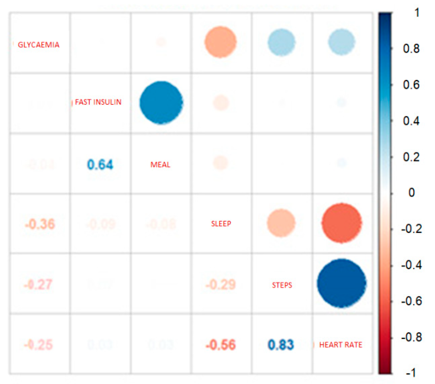
Sometimes one feature is directly dependent on one or more others, and therefore the information in the two (or more) data series is eminently equal and considering both might add noise to the analysis. In this sense, calculating a correlation matrix can help in determining whether redundant information exists.

So, it is possible to express the correlation factor between features, taken in pairs. A positive value implies a positive association. In this case, large (or small) values of one variable tend to be associated with large (or small) values of the other. A negative value of the correlation factor implies a negative or inverse association.

If two variables have a high correlation factor, it is possible to conclude that both have the same information (redundant) and therefore to eliminate one of them in order to reduce repetitious data. For this purpose, the corrplot routine (https://cran.r-project.org/web/packages/corrplot/vignettes/corrplot-intro.html) [49], contained in R software (https://www.r-project.org/), easily offers the correlation matrix, which could shed some light on this issue. In Figure 1, the correlations between the features considered in this work are expressed. With this technique, relations by pairs can be articulated.

From the data depicted in Figure 1, it is possible to draw some conclusions. There is a high correlation between insulin and meal, due to the fact that, most of the time, both events occur simultaneously. However, in hyperglycemia, there are solely insulin injections without meal ingestion (in order to lower glucose levels) and, in hypoglycemia, the patient needs to ingest a meal (mainly sugar) while insulin is never injected, and for this reason both insulin and meal have to be taken into account.

In addition, the correlation between glycemia and both insulin and meals are close to zero. This makes sense because a proper insulin dose completely compensates for hyperglycemia caused by ingestion. Blood sugar levels and exercise have, as expected, a negative correlation, and there is also a negative correlation between heart rate.

Continuing with the analysis, exercise (steps) and heart rate are highly correlated, as is reasonable. The correlation is not complete because in some situations it is possible to experience tachycardia or bradycardia under stress or sharp glycemic oscillations [50]. In addition, it is noted that there is an inverse correlation between heart rate and sleep, due to the bradycardia during sleep. In the same way, the same inverse relation can be found between exercise and sleep, for obvious reasons. So, as the inverse correlation between heart rate and sleep is stronger than the correlation between exercise and sleep, exercise could be considered as a feature reflected in heart rate values. Nonetheless, in the following study, no variable will be excluded; however, the preceding considerations could lead to the elimination of one or another feature in order to lighten the calculation tasks.

7.2. Feature Selection Results

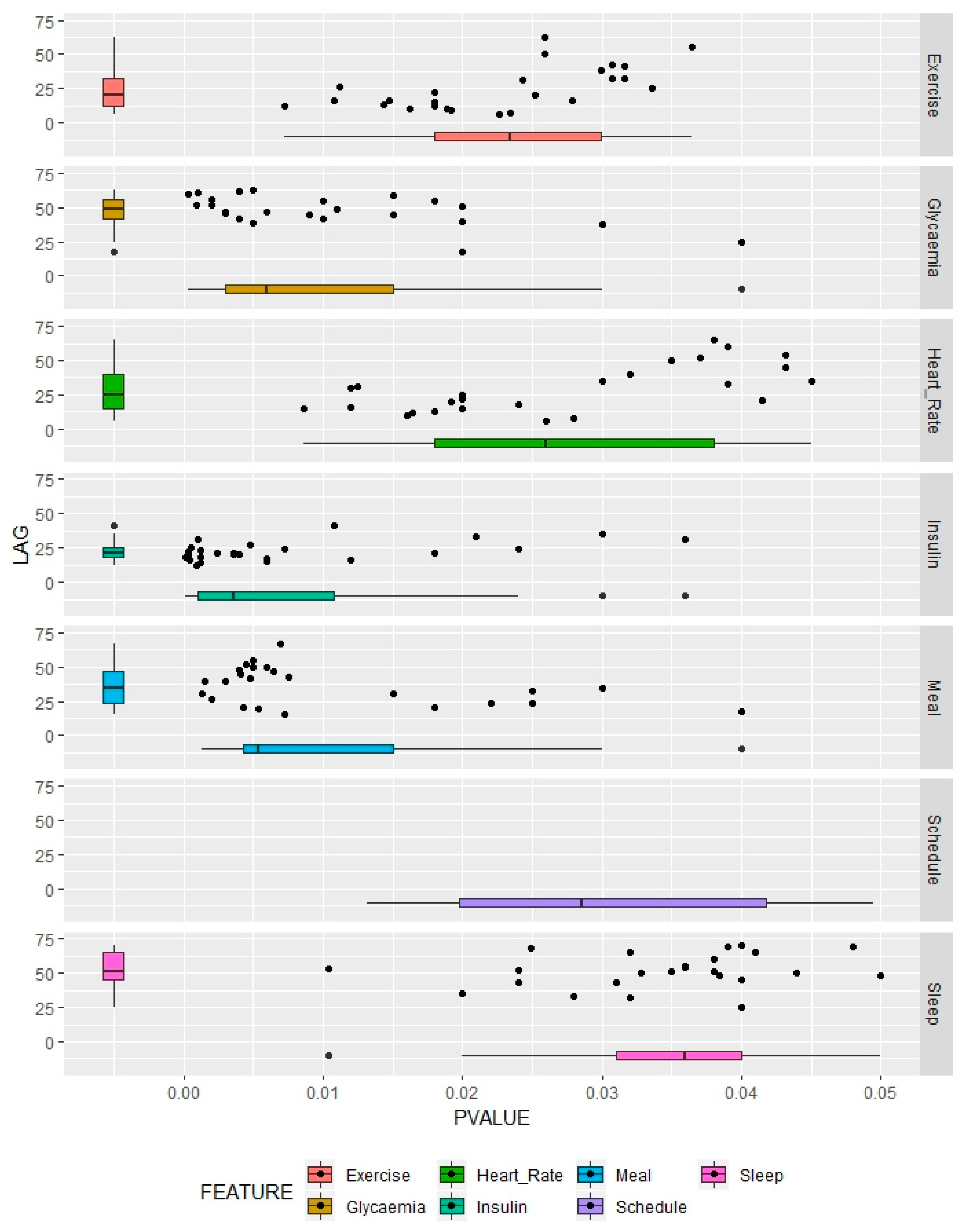
SISAL was put into effect using the SISAL package, (https://cran.r-project.org/web/packages/sisal/index.html) a library specially programmed for the so-called mathematical software R. It has been applied to a feature set composed of each of the 25 samples of the lagged variables: glycemia, insulin, meal, exercise, heart rate, and sleep, taking into account the past 75 values (as the sample frequency is 1 value per 5 min, we are considering a past window of 375 min, 6.25 h). In addition to the lagged values, we introduced schedule; this feature was registered as the hour and minute when glycemia was recorded.

The results are shown in Figure 2. For each lagged feature and each patient, we choose an optimum value, taking into account the significance, expressed by the p-value obtained using SISAL after evaluating a Z-score test [51], and the corresponding associated lag of that feature. The lower the p-value, the more significant the feature, considering a specific range of past data values. As schedule is not a lagged feature, for each patient the associated timestamp is taken into account, resulting in a p-value only.

Distributions of results are also expressed with boxplots. For this purpose, we can know the median value of the chosen lag results and have an idea of the dispersion of the performance. The same reasoning can be applied to the p-values to consider whether a feature is more or less important generally and show how it differs in importance between people participating in the study.

Values that are more concentrated around the median indicate that a certain feature behaves in the same way among members of the population, and high dispersion points to diverse responses between different diabetic people.

Table 2. Past values and p-value for each feature. Median values and standard deviation.

Feature	Past Values (Measures)		Past Values (Minutes)		p-Value
	Median	Std. D.	Median	Std. D.	Median	Std. D.
Insulin	21	7.08	105 (1.75 h)	35.40	0.00360	0.01011
Meal	35	13.88	175 (2.91 h)	69.40	0.00540	0.01030
Glycemia	49	11.27	245 (4.08 h)	56.35	0.00621	0.00992
Exercise	20	13.88	100 (1.66 h)	69.40	0.02340	0.01030
Heart Rate	25	17.19	125 (2.08 h)	85.95	0.02682	0.01154
Sleep	51	12.54	255 (4.25 h)	62.70	0.03721	0.00896
Schedule	–	–	–	–	0.02864	0.01254

summarizes the median values of the lag and p-value corresponding to each feature and their dispersion expressed by the standard deviation.

7.3. Relevance and Discussion of Historical Data

7.3.1. Global Overview and Importance Rank

Considering the p-values, the most influential feature is insulin, followed by meal. Glycemia takes third position in the ranking because it reflects the influence of all the relevant features at the same time. Continuing, and belonging to a separate influential group, we can find heart rate and sleep, which are significantly less important. Schedule is in this group, with a discrete influence.

Hereafter, a deeper analysis will be carried out.

7.3.2. Glycemia

First is the discussion of the main variable with its lagged values. Thus, this variable will be the predicted feature and also an input variable in a predictive model (taking into account its past values).

In the importance ranking, glycemia takes third position. Although some autoregressive models take into account only glycemia and simply the past nine values (barely half an hour, in [52]), these choices are not properly contended. In our study, the results indicate that around 4 h (49 past measures) can be a proper past window to take into account. We need to consider that this feature involves many other circumstances that can affect glycemia, so we can consider this past 4 h as a summary of the influential past all at once.

7.3.3. Insulin

Insulin is the most influential feature, according to the p-values, followed by meal. In this sense, we can appreciate that the standard deviation is smaller in the case of insulin, which is because the behavior of this one feature is more constant among people.

Insulin increases importance at 21 past values, which means 1.75 h. This is reasonable, since we are referring to fast-acting insulin (boluses), and this type of insulin usually has its main effect during two and a half hours, with a maximum at 90 min [53]. Anyway, we can see some data that point to a longer, residual action. This concept has been taken into account several times in the scientific literature; it is called insulin on board (IOB) and means the amount of insulin that is currently in the body (and therefore continues to act). It involves basal insulin and remaining fast-insulin, which can act with low (but noticeable) intensity for several hours. It has been assumed to have a remarkable effect during the past eight hours [54], although other research points to an acting range of the previous five to eight hours [55].

7.3.4. Meal

Meal is the second most important variable. In this case, it is seen to be more variable from one patient to another, which makes sense as the absorption of meals is different depending on the nutritional composition and on the metabolism of each person. Thus, meals with a higher fat percentage will have an influence in glycemia later [56,57]; on the other hand, the intake of fiber can slow down the absorption of carbohydrates [58].

The results offer a good past window with 35 past values, in other words, 2.91 h. This is consistent with previous literature, which estimates it in 3.27 h [32].

7.3.5. Exercise

Continuing with exercise, its influence on glycemia evolution has been studied so far as it increases the demand for glucose and raises the insulin sensitivity [8]. It is highly linked to heart rate, and due to this strong correlation, exercise data could be excluded since it can be considered to be included in the heart rate time series, but this discussion needs to be taken cautiously and is left for consideration, in a general view, depending on the dataset, the patients, and their habits.

Relevant past values of exercise data include 1.75 h (21 past values). This result seems to be coherent with literature related to the influence of sports [59] and it presents a wide variability, as it covers a wide range of different sports and intensities. Anyway, exercise still has an effect up to 48 h later [60]. According to the results, we can distinguish a group of people who practice medium-to-high intensity sports and a minority who practice more leisurely physical activity.

7.3.6. Heart Rate

Heartbeat is the fifth variable. If an increase in heart rate is not related to physical activity, it could be generated by stress situations [61]. Moreover, variation of pulse can also be indicative of a hypoglycemic episode [62]; the relationship with hyperglycemia has also been studied [63].

It can be noted that the correlation between exercise and heart rate is high in short term (patients with high-intensity exercise), but this interaction is not exactly followed in patients with relevant past lags of both variables. In this latter case, it can be assumed that the previously mentioned reasons influence heart rate more than physical activity.

Therefore, heart-rate reactions are very variable from a person to other, which is the reason why results that offer relevant past data are included in a window of 2.08 h. Usually, recent events that change fast glycemia (unexpected hypoglycemia or hyperglycemia, abrupt exercise) involve an immediate change of pulse, but the results point to the fact that some changes of heartbeat are not due to any cause that alters glycemia.

7.3.7. Sleep

The inclusion of sleep is another novelty of this paper. The influence of the number of sleeping hours is discussed here, considering that a lack of rest implies a rise of some stress hormones which are hyperglycemic.

As the influence is low, according to the p-values obtained, and is fairly variable from person to person, sleep deprivation has been pointed to as a cause of insulin resistance [12,64], which leads to hyperglycemia in diabetic patients.

The discussion of lag points to a discrete influence sustained over time. The results suggest that this value is more than 4 h, but this can vary under other circumstances.

7.3.8. Schedule

Circadian rhythms and the importance of having a schedule and a routine in order to manage diabetes are well known [65] but have not been included in a prediction algorithm yet. Humans have biological cycles which oscillate around 24 h. These 24-h rhythms are driven by a circadian clock and have been widely observed in plants and animals. Although circadian rhythms are endogenous, they are adjusted (entrained) to the local environment by external causes, which include light, temperature, and schedule.

Schedules tend to be similar from one day to another. At least, from one week to another, it is possible to identify a pattern, especially in the case of diabetic patients, since this is generally helpful to control their diabetes. Several tasks are usually carried out routinely at the same hour, like working, eating, practicing sports, or injecting insulin.

In addition, the effectiveness of insulin, measured by the insulin correction factor [48] (sometimes called an insulin sensitivity factor) can change with time, depending on factors such as how many hours ago the patient ate [66], and these hours can obey a pattern during the daytime. Disruptions in the circadian cycle could lead to insulin resistance [67]. Moreover, the dawn phenomenon [68], an increase of glycemia before awakening due to stress hormones, is a well-known usual event and is highly linked to schedule.

Unfortunately, schedules tend to differ from one person to another, which explains the wide variability that we can find in this feature. Anyway, the p-values indicate that this is not a critical variable. In this case, we have not used lags as this is a variable with a pattern, taking values from 00:00 to 24:00 consecutively, and therefore it does not make sense to study the variable lagged.

8. Conclusions

Glycemia prediction is the first step toward an artificial pancreas. However, such prediction has to be complete, reliable, and accurate. For this purpose, the most complete characterization of the patient needs to be performed.

Therefore, first we need to introduce some biometric devices, such as CGM and smart bands, thus making it possible to collect the variables needed to predict blood glucose levels. Due to the lack of previous works, a remarkable monitoring campaign has been carried out, overcoming the limitations of the former studies. This complete experiment constitutes a novelty itself and will be a cornerstone of future investigation to be performed by the authors.

In addition to insulin, meals, and past glycemia values, some of these new recorded features such as schedules, sleeping time, and heart rate were found to be influential in glucose levels, and in this paper their importance has been ranked, thus providing an overview of their influence.

With this, SISAL offered results on the subject of importance but also on the number of past values that need to be taken into account. This is a crucial idea in order to ease the execution of the forecasting algorithm and its computational effort. In this sense, we have results that indicate that the most remarkable variables are insulin, meal, and past glycemia followed by exercise and then heart rate, sleeping time, and schedule. The set of features will depend on how demanding the chosen algorithm is and the power of the device which is computing the prediction.

In addition, the conclusions express that some variables noticeably show the same behavior between diabetic people (like insulin) and others display characteristics depending on the specific person. This is interesting in order to presume the behavior of a variable or study a particular performance according to each patient.

With this, a proper basis on which future works can be carried out has been set, and it leads to some forthcoming research lines. As future work, and as a direct application of the study presented in this manuscript, we will use this method to achieve reliable and efficient predictive algorithms for glucose level prediction in DM1 patients, analyzing the different role of each feature. Moreover, the set of 25 subjects which was considered in the measurement campaign will be expanded, trying to monitor up to 50 patients. In conclusion, novel forecasting strategies are awaiting, and the results of this paper point to the necessity of a patient-dependent forecasting model, since it seems essential, at least for some features, the creation of person-based approaches.