Analysis of Influencing Factors and Trend Forecast of Carbon Emission from Energy Consumption in China Based on Expanded STIRPAT Model

Abstract

With the convening of the annual global climate conference, the issue of global climate change has gradually become the focus of attention of the international community. As the largest carbon emitter in the world, China is facing a serious situation of carbon emission reduction. This paper uses the IPCC (The Intergovernmental Panel on Climate Change) method to calculate the carbon emissions of energy consumption in China from 1996 to 2016, and uses it as a dependent variable to analyze the influencing factors. In this paper, five factors, total population, per capita GDP (Gross Domestic Product), urbanization level, primary energy consumption structure, technology level, and industrial structure are selected as the influencing factors of carbon emissions. Based on the expanded STIRPAT (Stochastic Impacts by Regression on Population, Affluence, and Technology) model, the influencing degree of different factors on carbon emissions of energy consumption is analyzed. The results show that the order of impact on carbon emissions from high to low is total population, per capita GDP, technology level, industrial structure, primary energy consumption structure, and urbanization level. On the basis of the above research, the carbon emissions of China′s energy consumption in the future are predicted under eight different scenarios. The results show that, when the population and economy keep a low growth rate, while improving the technology level can effectively control carbon emissions from energy consumption, China′s carbon emissions from energy consumption will reach 302.82 million tons in 2020.

1. Introduction

According to the fourth IPCC assessment report, the average surface temperature has risen by about 0.74 °C in the past 100 years [1]. Global climate change is mainly caused by greenhouse gases such as carbon dioxide and methane emitted by human activities. The warming effect of carbon dioxide is the most clear. In order to reduce carbon dioxide emissions and the negative impact of human activities on the environment, the international community has made many efforts in this century. China is the largest developing country whose science and technology are inferior to developed countries. Additionally, its economic development largely relies on traditional energy, so the environmental problems and energy crisis need to be solved urgently in China [2]. China is also a big energy-consuming country. Under the background of global low carbon emission reduction, China has an obligation to contribute to the development of environmental friendliness.

As for the influencing factors of carbon emissions, scholars at home and abroad have made fruitful research. The representative research results are driving force analysis based on the IPAT equation and driving factor analysis based on the Kaya model. Ehrlich et al. put forward the IPAT equation, believing that the driving force of carbon emissions is the comprehensive effect of population size, the economic development level, and scientific and technological progress [3]. Dietz et al. combined stochastic theory with the IPAT model and established the STIRPAT model. He introduced the index into the model so that the model could be used to analyze the non-proportional impact of human factors on the environment [4]. Kaya, who is a Japanese scholar, established a mathematical model to reflect the quantitative relationship between population, economy, energy, and carbon dioxide produced by human activities. He believed that the total amount of carbon dioxide produced by social and economic activities in a region was equal to the product of factors such as total population, per capita GDP, energy intensity, and carbon emissions per unit energy consumption [5]. Wang et al. decomposed the influencing factors of carbon emissions by logarithmic mean Dirichlet decomposition (LMDI). The results showed that energy intensity was the most important factor to reduce carbon emission [6]. Wang Feng and others used the logarithmic average Divisia index decomposition method to study the growth rate of carbon dioxide emissions from China′s energy consumption. He thought that per capita GDP growth was the greatest factor affecting the increase of carbon emissions, and that the decrease of energy intensity in the production sector was the most important factor to restrain the increase of carbon emissions [7].

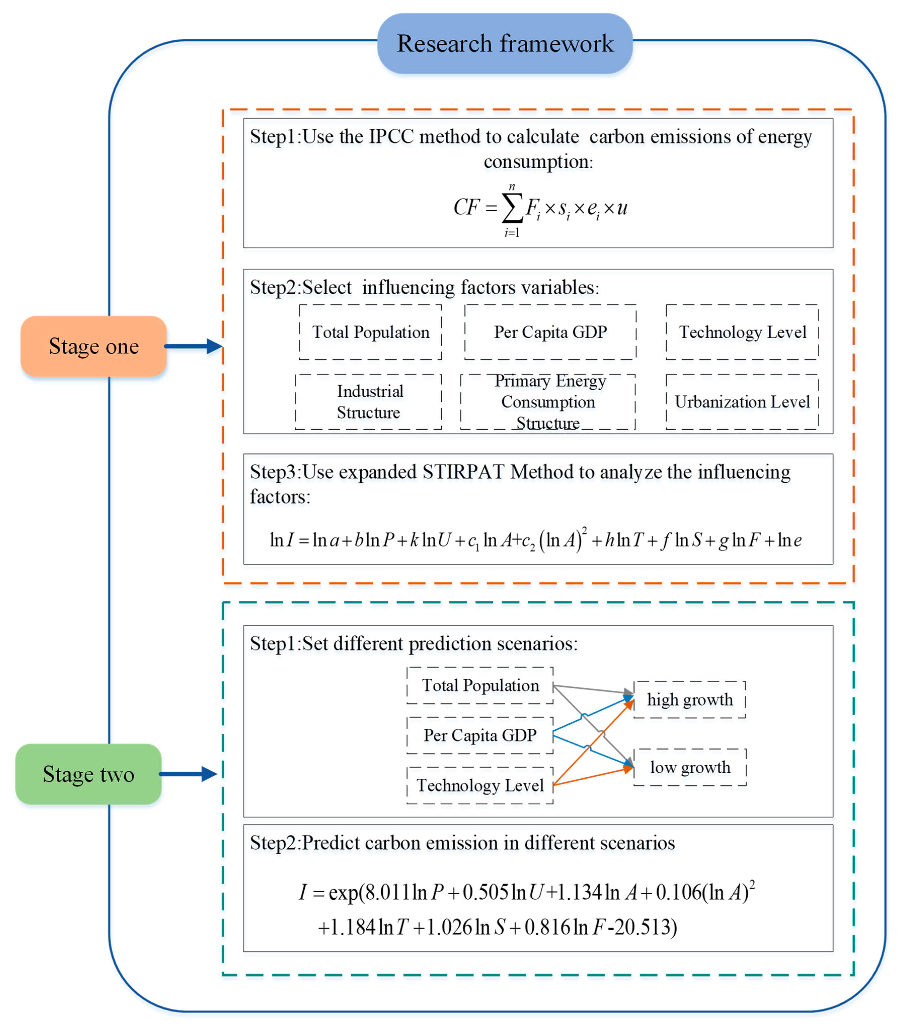
Research shows that different factors have different effects on carbon emissions, so it is necessary to further explore the factors affecting carbon emissions. In view of the shortcomings of previous studies, this paper uses the expanded STIRPAT model to analyze the impact of population size, affluence, primary energy consumption structure, technology level, industrial structure, and urbanization level on total carbon emissions. On the basis of factor analysis, the three most influential factors are taken as variables to set different scenarios. In addition, the carbon emissions of China′s future energy consumption under different scenarios are predicted and analyzed. The research structure of the article is shown in Figure 1. Within the figure, b, k, c, h, f, and g are elastic coefficients. Descriptions of other symbols are shown in following article.

2. Establishment of Influencing Factors Regression Model

2.1. Sources of Data

Energy consumption data are from the China Energy Statistics Yearbook (1996–2016) [8]. Population, GDP, urban population, and output value of secondary industry all come from the “China Statistical Yearbook” (1996–2016) [9].

2.2. Introduction of the Modeling Method

2.2.1. Introduction of the Carbon Emission Calculating Method

This paper analyzes carbon emissions from energy consumption in China. Considering the availability of data and the purpose of research, the IPCC method is adopted in this paper. The selected energy consumption categories are raw coal, washed coal, coke, coke oven gas, other gas, crude oil, gasoline, kerosene, diesel oil, fuel oil, liquefied petroleum gas, refinery dry gas, and natural gas. The calculation formula is shown below.

$$CF={\displaystyle \sum _{i=1}^n{F}_i}\times s_i\times e_i\times u$$

(1)

F_i is the total energy consumption per ton. s_i is the standard coal coefficient for energy conversion, as shown in

Table 1. Standard coal coefficient for 13 energy conversions.

	Standard Coal Coefficient	Energy Types	Standard Coal Coefficient
raw coal	0.7143	kerosene	1.4714
washed coal	0.9000	diesel oil	1.4571
coke	0.9714	fuel oil	1.4286
coke oven gas	0.5926	liquefied petroleum gas	1.7143
other gas	0.3214	refinery dry gas	1.5714
crude oil	1.4286	natural gas	1.2128
gasoline	1.4714

. $e_i$ is the carbon emission factor of each energy source. The energy carbon emission coefficients used in this paper refer to the various energy carbon emission coefficients in the 2006 IPCC National Greenhouse Gas Emission Inventory Guidelines, as shown in

Table 2. Carbon emission coefficient for 13 energy types.

Energy Types	Carbon Emission Coefficient	Energy Types	Carbon Emission Coefficient
raw coal	0.7559	kerosene	0.5714
washed coal	0.7559	diesel oil	0.5921
coke	0.855	fuel oil	0.6185
coke oven gas	0.3548	liquefied petroleum gas	0. 5042
other gas	0.3548	refinery dry gas	0.4602
crude oil	0.5857	natural gas	0.4483
gasoline	0.5538

. Since the statistical unit of each energy consumption is not meaningful, u is the unit conversion coefficient.

2.2.2. Introduction of Influencing Factors Analysis Method

The IPAT (I = Human Impact, P = Population, A = Affluence, T = Technology) model is widely used in the research of carbon emission related issues. The IPAT model was first proposed by American ecologists Ehrlich and Commoner to study the relationship between human activities and the natural environment. The major variables are population size (P), affluence (A), technology level (T), and environment (I) [10]. It has been widely used by scholars to analyze the influencing factors of environmental change since it is simple and easy to understand. However, the factors leading to environmental problems are complex. The IPAT model only involves three influencing factors, which cannot fully reflect the actual problems. The model can only analyze the problem by changing one factor while keeping other factors fixed, so that the influence of independent variables on dependent variables is proportional. However, this is not in line with the actual situation. In order to make up for the deficiency of the IPAT model, York and other scholars put forward the STIRPAT model on the basis of this model [11], which is expressed as follows.

$$I=a{P}^b\times A^c\times T^{d}e$$

(2)

In the formula, a is the coefficient of the model, b, c, and d are the index of population size, affluence degree, and technology level, respectively, and e is the random error term. In practical application, according to the STIRPAT model, the elasticity of influence factors on the environment is obtained by taking a natural logarithm on both sides of the equation. The logarithmic form is as follows.

$$\ln I=\ln a+b\ln P+c\ln A+d\ln T+e$$

(3)

Among them, b, c, and d are the elasticity coefficients of the population, affluence, and the level of technology, and ln a is a constant term.

In order to analyze the influencing factors of carbon emission intensity in China, this paper introduces six indicators: total population, urbanization level, per capita GDP, technology level, industrial structure, and primary energy consumption structure to extend the original STIRPAT model. The expanded STIRPAT model is expressed below.

$$\ln I=\ln a+b\ln P+k\ln U+c\ln A+h\ln T+f\ln S+g\ln F+\ln e$$

(4)

Among them, I represents the total carbon emissions from China′s energy consumption, P represents the total population, U represents the urbanization level, A represents the per capita GDP, T represents the level of technology, S represents the industrial structure, and F represents the primary energy consumption structure. b, k, c, h, f, and g are elastic coefficients, which indicate that, when P, U, A, T, S and F change by 1%, the carbon emissions will change b%, k%, c%, h%, f%, and g%, respectively.

The explanations of each variable are given in

Table 3. The explanations of variables.

Variable	Symbol	Variable Description	Unit
carbon emission	I	total carbon dioxide emissions	ten thousand tons
population size	P	total population	ten thousand
affluence	A	per capita GDP	yuan
technology level	T	energy intensity	–
urbanization level	U	urbanization rate	%
industrial structure	S	the proportion of the output value of the secondary industry	%
primary energy consumption structure	F	the proportion of coal consumption in primary energy consumption	%

.

Technology level refer to energy intensity. Energy intensity is energy consumption per unit of GDP, which reflects the input-output characteristics of the energy system, and reflects the overall efficiency of energy economic activities.

The urbanization level is expressed by the urbanization rate, that is, the proportion of urban population to the permanent population. The urbanization level is one of the important factors affecting carbon emissions. Cities are the concentration areas of population, transportation, industry, and other resources, as well as energy consumption and carbon emissions [12].

The industrial structure is explained by the proportion of the output value of the second industry in the total output value of that year. Among the three major industries, the secondary industry consumes the largest energy, especially the heavy industry.

The structure of the primary energy consumption is the proportion of coal consumption in primary energy consumption in that year. China′s energy consumption structure is still dominated by coal, and coal and other fossil energy consumption is the main reason for carbon dioxide production.

In order to test whether there is an inverted U-shaped curve between economic growth and carbon emissions, the ln A in model (4) is decomposed into ln A and (ln A) ² [13]. The model is adjusted below.

$$\ln I=\ln a+b\ln P+k\ln U+c_1\ln A+c_2{\left(\ln A\right)}^2+h\ln T+f\ln S+g\ln F+\ln e$$

(5)

c₁ and c₂ are coefficients of the logarithm of per capita GDP and logarithm quadratic of per capita GDP, respectively.

From Equation (5), the elasticity coefficient EE_IA of per capita GDP to carbon emissions from energy consumption can be obtained as follows.

$$E{E}_{IA}=c_1+2c_2\ln A$$

(6)

If c₂ is negative, there is an inverted U-shaped curve between per capita GDP and carbon emissions.

In data regression, because the nature and unit of each variable are different, if the original data is directly used for regression, it will result in unfair regression. Therefore, before using principal component analysis, the data should be standardized. The standard processing method adopted in this paper is the Z-score processing method [14].

2.3. Regression Model Results

2.3.1. Results of China′s Energy Consumption Carbon Emissions

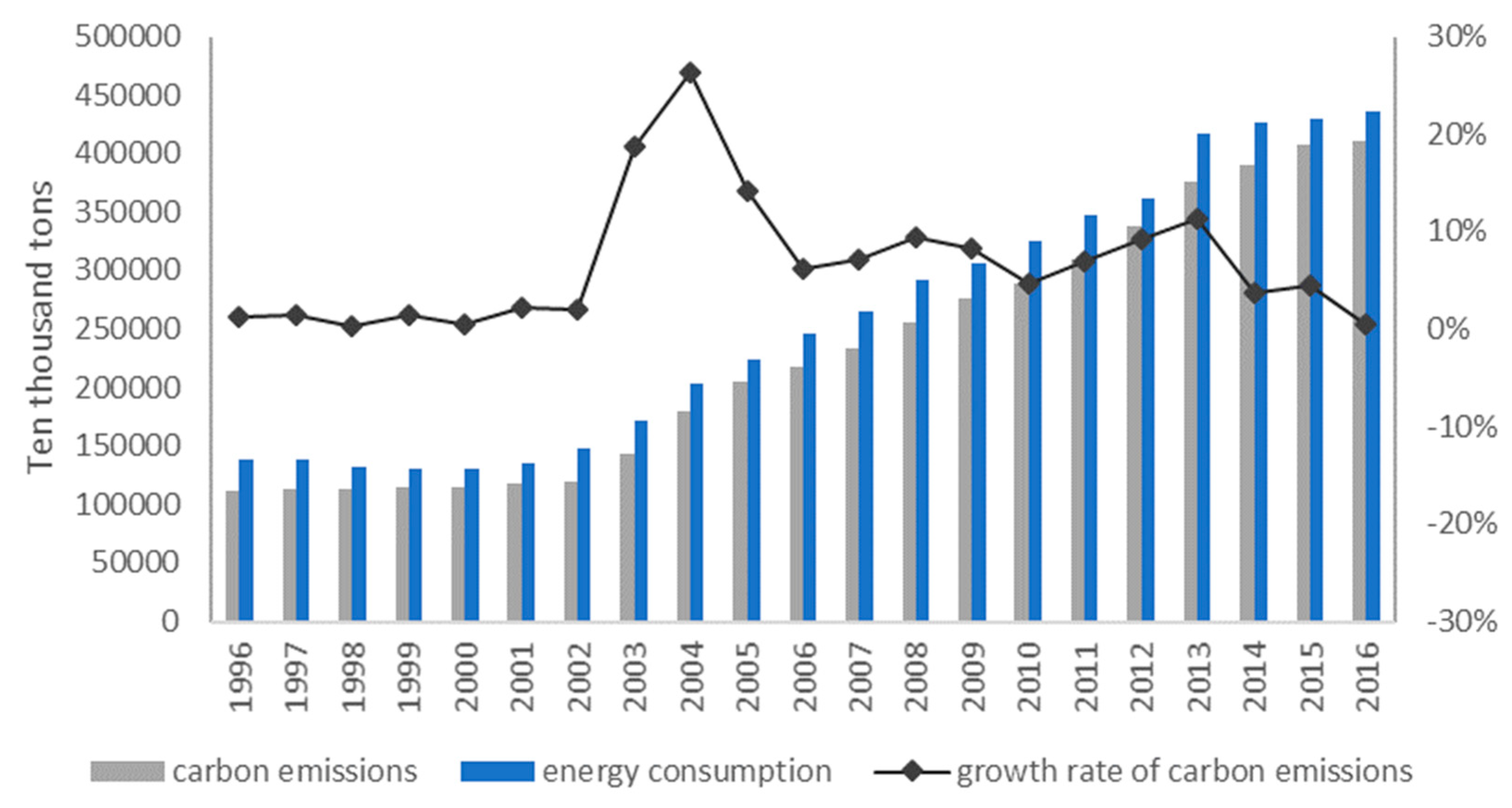
According to the China Energy Statistics Yearbook (1996–2016) and Formula (1), China′s energy consumption and carbon emissions from 1996 to 2016 are calculated as shown in Figure 2.

As can be seen from the figure, since 1996, China′s total energy consumption has maintained a growing trend. China′s total energy consumption in 1996 was 138.948 million tons, while, in 2016, it was 435.819 million tons, which reached an increase of 213.66%. Similarly, carbon emissions from China′s energy consumption were increasing. Before 2003, the growth rate was low and stable at 2%. However, the growth rate in the three years from 2003 to 2005 exceeded 15%, of which the growth rate in 2004 reached 26.25%. After 2005, the growth rate has decreased slightly, but the carbon emissions are still increasing. From 111.263 million tons in 1996 to 410.052 million tons in 2016, it increased by 268.54% in 20 years.

2.3.2. Results of the Regression Model

The least squares regression is performed on the variables lnP, lnU, lnA, (lnA)², lnT, lnS, and lnF. The model test results include the adjustable coefficient R² = 0.71505, the F value is 43.31292, and the p value is 0.00000 < 0.05. The multivariate regression parameters are estimated as shown in

Table 4. Estimation of multivariate regression parameters.

Variable	Coefficient	Standard Error	t-Statistic	Probability	VIF
C	8.07×10−8	0.0131	6.17×10−6	1.0000	−
lnP	1.8444	0.7040	2.6199	0.0212	2759.3270
lnU	−1.8825	0.7706	−2.4430	0.0296	2951.6632
lnA	−0.7634	3.5876	−0.2128	0.8348	1754.8335
(lnA) 2	2.5871	3.3737	0.7669	0.4569	109.1082
lnT	−0.7992	0.1163	−6.8732	0.0000	75.0465
lnS	0.0170	0.0668	0.2549	0.8028	24.1146
lnF	0.0163	0.0841	0.1943	0.8489	19.7655

, and the value p of the variables ln A, ln T, and ln S are all greater than the significance level of 0.05. The Variance Inflation Factor (VIF) is calculated on the basis of multiple explanatory variables to assist the regression equation, and reflects the severity of multicollinearity between explanatory variables. It is generally believed that there is a serious multiple collinearity between explanatory variables and residual explanatory variables when VIF is greater than 10. Additionally, the multiple collinearity between explanatory variables will affect the results of least squares regression [15]. In this study, the variable VIF values for each indicator are shown in Table 4. There are multiple collinearity between variables. The main methods to eliminate multicollinearity are partial least squares [16], principal component regression [17], and ridge regression [18]. In this study, principal component regression is used.

Before eliminating multiple collinearity by principal component regression, the independent variables ln P, ln U, ln A, (ln A) ², ln T, ln S, and ln F should be tested by KMO (Kaiser-Meyer-Olkin) test and Bartlett sphericity test. The two tests can confirm whether the above variables are suitable for principal component regression [19]. This can be seen from

Table 5. KMO test and Bartlett sphericity test.

Kaiser-Meyer-Olkin Measure of Sampling Adequacy		0.747
Bartlett′s Test of Sphericity	Approx. Chi-Square	502.132
	df	21
	sig	0.000

. The result shows that KMO = 0.747. The Bartlett sphericity test has a significant value less than 0.05, so we should reject the zero hypothesis. Additionally, consider that the correlation coefficient matrix cannot be a unit matrix. Therefore, there is correlation between the original variables. This indicates that these seven independent variables are suitable for principal component analysis.

This paper uses SPSS22.0 software to carry out principal component analysis. The eigenvalues of each factor must be greater than 1. The contribution rate of cumulative variance is shown in

Table 6. The cumulative variance contribution rate.

Component	Eigenvalue	Percentage of Variance of Initial Eigenvalue	Cumulative Percentage	Total	Percentage of Square Sum Loading Variance Extracted	Cumulative Percentage
1	5.273	75.336	75.336	5.273	75.336	75.336
2	1.572	22.451	97.787	1.572	22.451	97.787
3	0.137	1.958	99.745
4	0.011	0.152	99.897
5	0.007	0.100	99.997
6	0.000	0.003	100
7	7.378×10−6	0.000	100

Extraction method: Principal component analysis.

and the principal component load matrix is shown in

Table 7. Principal component load matrix.

Variable	1	2
lnP	0.989	0.124
lnU	0.987	0.146
lnA	0.989	0.096
(lnA)2	0.990	0.072
lnT	0.991	−0.057
lnS	−0.611	0.750
lnF	0.084	0.977

. The contribution rate of variance of the first principal component extracted is 75.336% and, of the first two, is 97.787%, which means it meets the requirement of principal component extraction. Therefore, this study extracts two principal components Z1 and Z2 after seven independent variables of principal component analysis.

According to Table 7, we can get the principal component coefficient, as shown in

Table 8. Principal component coefficient.

Variable	1	2
lnP	0.187	0.079
lnU	0.187	0.093
lnA	0.188	0.061
(lnA)2	0.188	0.046
lnT	0.188	−0.036
lnS	−0.116	0.477
lnF	0.016	0.622

. With the result of principal component analysis, the regression equations of Z1 and Z2 can be established.

$$\begin{gathered} Z1=0.187\ln P^{\ast }+0.187\ln U^{\ast }+0.188\ln A^{\ast }+0.188{\left(\ln A^{\ast }\right)}^2+0.188\ln T^{\ast }-0.188\ln S^{\ast }+0.016\ln F^{\ast } \\ Z1=0.079\ln P^{\ast }+0.093\ln U^{\ast }+0.061\ln A^{\ast }+0.046{\left(\ln A^{\ast }\right)}^2-0.036\ln T^{\ast }+0.477\ln S^{\ast }+0.622\ln F^{\ast } \end{gathered}$$

Establishing regression equation as follows,

$$\ln I^{\ast }={\beta }_0+{\beta }_{1}Z1+{\beta }_{2}Z2$$

(7)

β₀ is a constant term. β₁ and β₂ are coefficients.

The regression result is shown in

Table 9. Component coefficient.

Coefficient	Non-Standardized Coefficient	Standard Error	Standardized Coefficient	t	Significant	VIF
β0	−	0.046	−	0	1.000	−
Z1	0.769	0.047	0.793	20.450	0.000	1.000
Z2	0.316	0.047	0.325	2.961	0.008	1.000

* means at 0.1 level. Therefore, the regression result is as follows.

. From Table 9, we can see that VIF is 1.000, so there is no multiple collinearity between the extracted two principal components. After calculating the score, we make a regression analysis with a standardized dependent variable ln I* and the adjusted R-squared is 0.823. The P value of the T-test of the constant term (β₀) is not significant, but the coefficient is very small and can be neglected. Therefore, it has no influence on this study. The T-test of Z1 and Z2 showed a significant difference.

$$\begin{array}{ll}\ln I^{\ast }& =0.793Z1+0.325Z2\\ & =0.412\ln P^{\ast }+0.711\ln U^{\ast }+1.656\ln A^{\ast }+1.826{\left(\ln A^{\ast }\right)}^2\\ & +2.266\ln T^{\ast }+0.752\ln S^{\ast }-0.205\ln F^{\ast }\end{array}$$

The above formula is a regression equation for standardized variables. According to the principle of standardization, the final regression equation can be obtained by restoring the data.

$$\begin{array}{c}\ln I=8.011\ln P+0.505\ln U+1.314\ln A+0.106{(\ln A)}^2\\ +1.184\ln T+1.026\ln S+0.816\ln F-20.513\end{array}$$

The regression results show that the order of impact on carbon emissions from high to low is population, per capita GDP, level of science and technology, proportion of secondary industry, primary energy consumption structure, and urbanization level. Their elasticity coefficients are 8. 011, (1.314 + 0.212ln A), 1.184, 1.026, 0.816, and 0.505, respectively. Among them, A is per capita GDP.

The coefficient of (ln A)² is positive, which indicates that there is no inverted U-shaped relationship between China′s economic growth and carbon emissions. With the economic growth, environmental pressures are increasing day by day, and there is no equilibrium inflection point yet.

3. Prediction of Carbon Emission Trend under Different Scenarios

3.1. Introduction of Prediction Model

Based on the simulation results of the STIRPAT model, the future carbon emissions of China are predicted. The prediction formulas are shown below.

$$\begin{array}{ll}I& =\exp (8.011\ln P+0.505\ln U+1.134\ln A+0.106{(\ln A)}^2+1.184\ln T\\ & +1.026\ln S+0.816\ln F-20.513)\end{array}$$

(8)

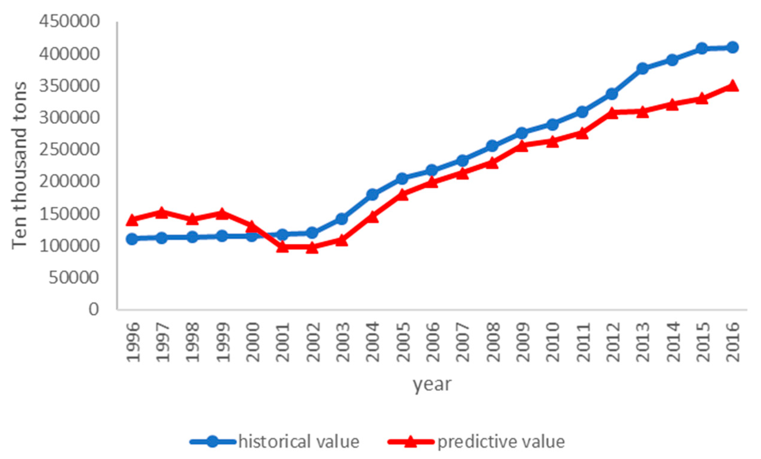
According to the historical population, per capita GDP, primary energy consumption, energy intensity, the proportion of secondary industry, and urbanization rate, this paper uses the above model to simulate the carbon emissions of China′s historical energy consumption, and makes regression between the simulated and historical values. The comparison chart is shown in Figure 3. The results show that the simulated R² reaches 0.9984. Therefore, it is feasible to use the above model to forecast the carbon emissions of energy consumption in China in the future.

3.2. Scenarios Setting

In the factor analysis above, population, per capita GDP, and the technological level are the three factors that have the greatest impact, respectively. Therefore, taking these three indicators as variables in the scenario and growth rate as scenario conditions, the specific scenario settings are shown in

Table 10. Scenario settings.

Scenario	Population	Per Capita GDP	Technological Level
scenario 1	low growth	low growth	high growth
scenario 2	low growth	low growth	low growth
scenario 3	high growth	low growth	high growth
scenario 4	high growth	low growth	low growth
scenario 5	low growth	high growth	low growth
scenario 6	low growth	high growth	high growth
scenario 7	high growth	high growth	low growth
scenario 8	high growth	high growth	high growth

.

3.3. Prediction of Carbon Emission Trend

According to the Development Strategy of the Development Research Center of the State Council and the Report of the Ministry of Regional Economic Research on the Forecast and Analysis of the Speed of Urbanization in China [No. 99 of 2017], the growth rate of urbanization in China slowed down from 2016 to 2050. The urbanization rates in 2020, 2030, 2040, and 2050 were 60.34%, 68.38%, 75.37%, and 81.63%, respectively [20]. In this way, we can deduce that the growth rate of the urbanization rate in each stage is 0.793%, and then calculate the urbanization rate of China in the coming years.

According to the national energy strategic action plan and related research, the slowdown of coal demand growth will become a new normal for the development of the coal industry. By 2020, 2030, 2040, and 2050, the proportion of coal in China′s primary energy structure will remain 62%, 55%, 53%, and 50% [21]. Similarly, it can deduce the primary energy consumption structure in different stages, and calculate the primary energy consumption structure in future years in China.

According to the Long-term Forecast of China′s Economy in the 21st Century, the proportion of the secondary industry output value to GDP in 2020, 2030, 2040, and 2050 is 50.2%, 48%, 45.3%, and 42.1%, respectively [22]. According to the same method mentioned above, we can predict the proportion of secondary industry output value in China in the coming years.

Based on the historical data of China from 1996 to 2016, the population growth rate and per capita GDP growth rate of each year are calculated. The maximum and minimum growth rates of population growth rate (1.13% vs 0.39%)and per capita GDP growth rate (13.64% vs. 6.12%) are used as their respective high and low growth rates, respectively, to estimate China′s future population and per capita GDP. The maximum and minimum of the energy intensity decline rate (14.26% vs. 1.75%) are selected as the high and low growth rates of technology, respectively. Additionally, the future technological level of China is estimated.

Based on the above scenarios, the carbon emissions from China′s energy consumption are predicted by using Formula (8). The calculation results are shown in Figure 4.

Table 11. Prediction of China′s energy consumption carbon emissions in different scenarios.

Scenario	2020	2030	2040	2050
S1	302.81	359.96	362.27	692.05
S2	337.72	552.06	704.77	835.34
S3	341.82	429.13	663.62	1123.48
S4	354.29	579.03	1285.48	1963.68
S5	355.61	562.59	1188.6	2103.72
S6	327.33	437.52	770.38	1351.39
S7	316.47	603.37	1547.23	3527.45
S8	368.43	733.56	2003.69	5532.06

Unit: million tons.

provides a forecast of carbon emissions from China′s energy consumption in 2020, 2030, 2040, and 2050.

4. Discussion

4.1. Discussion on Influencing Factors

Population size has the highest impact on carbon emissions, and the elasticity coefficient is as high as 8.011. It shows that if the population increases by 1%, the total carbon emissions will increase by 8.011%. China has a large population base, and its lifestyle and production activities depend on traditional energy. Population size has the most direct impact on carbon emissions. China is the largest manufacturing concentration country in the world. Developed countries have set up high-pollution and high-energy-consuming manufacturing links in China. Labor-intensive and high-carbon industries make the environmental pressure worse.

Per capita GDP is another important factor affecting China′s energy consumption carbon emissions. For every 1% increase in per capita GDP, energy consumption carbon emissions will increase (1.314 + 0.212l n A). It is the second important factor affecting China′s energy consumption carbon emissions. This shows that China′s economic development and social life are highly dependent on energy consumption.

The elasticity coefficient of the impact of technology level on carbon emissions from energy consumption is 1.184. For every 1% increase in energy intensity, carbon emissions from China′s energy consumption will grow by 1.184%. China′s energy consumption structure is dominated by coal, which leads to a large consumption of fossil energy and a large amount of carbon emissions when GDP increases.

Similarly, the industrial structure also plays an important role in China′s energy consumption carbon emissions. Regression results show that every 1% increase in the proportion of secondary industry output value will generate 1.026% carbon emissions. In China′s industrial structure, heavy industry and manufacturing industry occupy the main position. This kind of industrial structure with high energy consumption and emission has a negative impact on reducing carbon emissions from energy consumption in China.

The impact coefficient of primary energy consumption structure, especially coal consumption, on China′s carbon emissions is 0.816%. The current situation of energy consumption in China is that coal accounts for 60% of primary energy. China is one of the few countries in the world where coal is the most important energy resource. It is also one of the most polluted areas in the world because of coal combustion. The long-term high proportion of coal resources in energy consumption is also one of the main reasons for China′s high carbon emissions. Therefore, China needs to optimize its energy structure and vigorously develop low-carbon energy.

The level of urbanization is also a factor contributing to the increase of carbon emissions from energy consumption in China. The regression results show that an increase of 1% in the urbanization level will result in an increase of 0.505% in carbon emissions. From 29.37% urbanization in 1996 to 57. 37% in 2016, China′s urbanization level has developed rapidly in the past 20 years. Yet, with the advancement of urbanization, the demand for energy in urban buildings, transportation, and residential buildings is also increasing, which increases China′s carbon emissions.

4.2. Discussion on Trend Prediction

As can be seen from Figure 4, in scenario 1, when China maintains low population growth rate, low per capita GDP growth rate, and high-tech growth rate in the future, the growth rate of carbon emissions from energy consumption in China is the slowest. By 2050, the carbon emissions will be 692.05 million tons. In scenario 8, when the population and per capita GDP keep a high growth, and the technological progress rate keeps low growth, the growth of carbon emissions from energy consumption will be the fastest. There will be 5532.06 million tons of carbon emissions by 2050. It is also eight times higher than the result in scenario 1. By comparing Scenario 2, Scenario 3, and Scenario 6 with Scenario 1, we can find that, when the population keeps low growth, the per capita technological level keeps high growth, and the per capita GDP keeps high growth, while the growth rate of carbon emissions from energy consumption is the fastest. While, when the population and per capita GDP keep a low growth, the growth rate of energy consumption is the slowest when the technological level keeps a low growth. Therefore, reducing carbon emissions from China′s energy consumption should enhance the technological level and reduce energy intensity.

Comparing Scenario 4 with Scenario 8, when the population keeps a high growth and the technological level keeps a low growth rate, the carbon emissions of energy consumption can be effectively reduced by reducing the growth rate of per capita GDP. Therefore, in order to control China′s future carbon emissions, it is necessary not only to improve energy utilization technology and control the population, but also to reduce the growth rate of per capita GDP. This means that China should slow down its economic development in the future, change its mode of economic growth, and make its economic growth tend to a new normal.

5. Conclusions

First, this paper calculates the carbon emissions of energy consumption in China from 1996 to 2016, and then uses the STIRPAT model to decompose the influencing factors of carbon emissions of energy consumption and analyze the influence degree of different factors. This combines different scenarios to predict the future trend of carbon emissions from energy consumption in China.

(1)

During the two decades from 1996 to 2016, China′s energy consumption and carbon emissions of energy consumption showed an increasing trend. Among them, energy consumption increased by 213.66% and carbon emissions of energy consumption increased by 268.54%.

(2)

Among the factors affecting carbon emissions from energy consumption in China, population factors have the highest impact on carbon emissions, with an elasticity coefficient of 8.011. The impact of per capita GDP on carbon emissions is second only to that of the population. The high demand for energy in China′s economic development has greatly increased China′s carbon emissions from energy consumption. The order of impact degree is population quantity > per capita GDP > technology level > industrial structure > primary energy consumption structure > urbanization level.

(3)

There is no inverted U-shaped relationship between China′s economic growth and carbon emissions. Therefore, with economic growth, environmental pressures are increasing, and there is no equilibrium inflection point.

(4)

By forecasting the carbon emissions of China′s future energy consumption in different scenarios, we can see that the growth rate of China′s energy consumption carbon emissions is the slowest while maintaining low population growth rate, low per capita GDP growth rate, and a high-tech growth rate. When in the scenarios of high population growth rate, high per capita GDP growth rate, and a low-tech growth rate, the carbon emissions are the highest. Therefore, in order to reduce China′s energy consumption carbon emissions, we should not only control the population size and control the speed of economic development, but also improve energy utilization technology and reduce the dependence of economic development on energy.

References

- The Fourth IPCC Assessment Report. Available online: https://www.ipcc.ch/reports/ (accessed on 1 March 2019).
- Bei, X. Research on Temporal and Spatial Migration of Energy Consumption Carbon Footprint and its Influence Factors in China. Master’s Thesis, Anhui University of Finance and Economics, Bengbu, China, December 2016. [Google Scholar]
- Ehrlich, P.R.; Ehrlich, A.H. Population, Resources, Environment. Issues in Human Ecology; Freeman: San Francisco, CA, USA, 1970; pp. 89–157. [Google Scholar]
- Dietz TRosa, E.A. Rethinking the environmental impacts of population affluence and technology. Hum. Ecol. Rev. 1994, 1, 277–300. [Google Scholar]
- Kaya, Y. Impact of Carbon Dioxide Emission on GNP Growth: Interpretation of Proposed Scenarios; Presentation to the Energy and Industry Subgroup; Response Strategies Working Group, IPCC: Paris, France, 1989; pp. 1–25. [Google Scholar]
- Can, W.; Jining, C.; Ji, Z. Decomposition of energy-related CO2 emission in China: 1957–2000. Energy 2005, 30, 73–83. [Google Scholar]
- Feng, W.; Lihua, W.; Chao, Y. Study on the Driving Factors of Carbon Emission Growth in China′s Economic Development. Econ. Res. 2010, 2, 0629. [Google Scholar]
- China Energy Statistics Yearbook (1996–2016); China Statistics Press: Beijing, China, 1996–2016.
- China Statistical Yearbook (1996–2016). Available online: http://www.stats.gov.cn/tjsj/ndsj/ (accessed on 1 December 2017).
- Shuang, L.; Tao, D.; Xia, Q. Study on the Influencing Factors of Carbon Emission in China′s Construction Industry Based on Extended STIRPAT Model. Mod. Manag. 2017, 37, 96–98. [Google Scholar]
- Jingshui, S.; Zhirui, C.; Zhijian, L. Research on the Influencing Factors of China′s Low Carbon Economy Development—Based on the Expanded STIRPAT Model Analysis. Audit Econ. Res. 2011, 26, 85–93. [Google Scholar]
- Bangli, C.; Meiping, X. Analysis of the Influencing Factors of Carbon Emissions in China: An Empirical Study of STIRPAT-Alasso Model Based on Panel Data. Ecoeconomy 2018, 1, 20–24. [Google Scholar]
- Yue, P. Analysis of Driving Factors of Carbon Emission in Jiangsu Province Based on STIRPAT Model. Environ. Pollut. Prev. 2014, 36, 104–109. [Google Scholar]
- Gao, T. An Empirical Study on the Influencing Factors of Housing Prices in Nanjing. Econ. Res. Guide. 2019, 12, 125–127. [Google Scholar]
- Vu, D.H.; Muttaqi, K.M.; Agalgaonkar, A.P. A variance inflation factor and backward elimination based robust regression model for forecasting monthly electricity demand using climatic variables. Appl. Energy 2015, 140, 385–394. [Google Scholar] [CrossRef] [Green Version]
- Xu, O.; Fu, Y.; Su, H. A Selective Moving Window Partial Least Squares Method and Its Application in Process Modeling. Chin. J. Chem. Eng. 2014, 22, 799–804. [Google Scholar] [CrossRef]
- LV, F.; Liang, B.; Sun, W.J.; Wang, Y. Gas emission quantity prediction of working face based on principal component regression analysis method. J. China Coal Soc. 2012, 37, 113–116. [Google Scholar]
- Ngo, S.H.; Kemény, S.; Deák, A. Performance of the ridge regression method as applied to complex linear and nonlinear models. Chemom. Intell. Lab. Syst. 2003, 67, 69–78. [Google Scholar] [CrossRef]
- Wu, H.C.; Ai, C.H.; Yang, L.J.; Li, T. A Study of Revisit Intentions, Customer Satisfaction, Corporate Image, Emotions and Service Quality in the Hot Spring Industry. J. China Tour. Res. 2015, 11, 371–401. [Google Scholar] [CrossRef]
- Shantong, L. The Prediction and Analysis of the Speed of Urbanization in China. Development Strategy and Regional Economic Research Department of Development Research Center of the State Council. Available online: http://www.drc.gov.cn/n/20170824/1-224-2894327.html (accessed on 1 December 2017).
- Xianzheng, W. Wang Xianzheng reports on the development of coal industry in China University of Mining and Technology. Coal Eng. 2014, 7, 120. [Google Scholar]
- Jingwen, L. Long-term Forecast of China′s Economy in the 21st Century. Metall. Econ. Manag. 2000, 3, 4–7. [Google Scholar]
Figure 1.
The research structure of the article.
Figure 2.
China′s energy consumption and carbon emissions from 1996 to 2016.
Figure 3.
Historical and forecast values of China′s energy consumption carbon emissions.
Figure 4.
Prediction trends of carbon emissions in different scenarios.