Article

Systematic Simplified Simulation Methodology for Deep Energy Retrofitting Towards Nze Targets Using Life Cycle Energy Assessment

by
José Sánchez Ramos
1,
MCarmen Guerrero Delgado
2,
Servando Álvarez Domínguez
2,
José Luis Molina Félix
2,
Francisco José Sánchez de la Flor
1 and
José Antonio Tenorio Ríos
3,*
1
Department of thermal machines and engines, University of Cadiz, 11001 Cadiz, Spain
2
Department of energy engineering, University of Seville, 41004 Seville, Spain
3
Spanish National Research Council (CSIC), 28033 Madrid, Spain
*
Author to whom correspondence should be addressed.
Energies 2019, 12(16), 3038; https://doi.org/10.3390/en12163038
Submission received: 22 July 2019 / Revised: 2 August 2019 / Accepted: 5 August 2019 / Published: 7 August 2019
(This article belongs to the Special Issue Life Cycle Energy Assessment on Buildings)

Abstract

:
The reduction of energy consumption in the residential sector presents substantial potential through the implementation of energy efficiency improvement measures. Current trends involve the use of simulation tools which obtain the buildings’ energy performance to support the development of possible solutions to help reduce energy consumption. However, simulation tools demand considerable amounts of data regarding the buildings’ geometry, construction, and frequency of use. Additionally, the measured values tend to be different from the estimated values obtained with the use of energy simulation programs, an issue known as the ‘performance gap’. The proposed methodology provides a solution for both of the aforementioned problems, since the amount of data needed is considerably reduced and the results are calibrated using measured values. This new approach allows to find an optimal retrofitting project by life cycle energy assessment, in terms of cost and energy savings, for individual buildings as well as several blocks of buildings. Furthermore, the potential for implementation of the methodology is proven by obtaining a comprehensive energy rehabilitation plan for a residential building. The developed methodology provides highly accurate estimates of energy savings, directly linked to the buildings’ real energy needs, reducing the difference between the consumption measured and the predictions.

Graphical Abstract

1. Introduction

1.1. Context

The International Energy Agency shows the relevance of the building sector in energy consumption [1,2,3]. IEA reports show the buildings as the main concern to target in order to reduce energy consumption, since the building sector consumes a third of the final energy. Additionally, IEA reports highlight the known fact of the significant retrofitting interventions needed by the existing building stock as part of their energy saving plans [1,2,3]. Changes should soon become a reality, given the investments on rehabilitation initiatives which must be performed before 2030 to achieve the goal of renovating 60% of the building stock by 2050.
Along the same line, towards the achievement of tangible energetic improvements in the building sector, is the problem of energy poverty, specifically affecting the residential sector [4]. Energy poverty refers to the situation in which a household is unable to maintain a proper level of indoor thermal comfort, as a consequence of the combination of the following factors: Low income of the residents, high energy prices, usually accompanied by the housings’ poor energy efficiency [5]. In Europe, the average energy consumption for heating in residential buildings is high [6], the goal is to lower this consumption by 50 kWh/m2, in the future [7].
Reduction of energy consumption for residential buildings in Europe could be achieved by the retrofitting of the existing building stock, possibly allowing to increase their sustainability and to improve their operation by reducing energy consumption costs and facilitating their maintenance tasks. Assuring the life cycle of the buildings, the existing energy efficiency criteria need to be taken into consideration, as well as the consequential environmental impacts, the economic feasibility, and the residents comfort standards, to speed up the reduction of the energy consumption in the building sector [8].
Upgrading the existing building stock is closely related to the optimization of the buildings’ lifecycle. Therefore, a refurbishment project should take into account energy savings measures in the buildings’ constructive elements, air conditioning and ventilation systems, control system, renewable energy and user behavior in the development of innovative methodologies. Furthermore, the consideration of all the possibilities to improve energy efficiency and their combination becomes a must, in order to find profitable energy-saving plans.
Likewise, for the energy-saving plans to be realistic, the results after the implementation of the suggested methodologies should be linked with the values from the real buildings’ energy bills to validate the values estimated for the energy consumption and the corresponding economic savings correctly. It allows to obtain verifiable energy improvements with the implementation of the recommended measures, chosen by following the method proposed, which includes the premises mentioned of the validation of the simulation results with the buildings’ actual energy bills and the highest possible number of energy rehabilitation measures including all of the possible combinations of alternatives.

1.2. Conventional Procedures for Evaluating Energy Efficiency

The most common standard in Europe is the International Organization for Standardization ISO 50001 [9], focused on the improvement of the buildings’ energy performance, including energy efficiency, use, and consumption. This standard establishes the foundations for energy management systems and existing buildings. The system is based on achieving potential energy savings, starting with the buildings’ basic energy use and implementing several improvement measures to measure their impact. The main objective of the system is to obtain real building indicators and to compare them with the reference values. For example, a benchmark is established from the buildings’ energy consumption indicator, when each set of measures is implemented in a specific building and their effect is measured, then the resulting values are used to analyze and select the measures from an existing catalog to be applied on a different rehabilitation project.
The literature review shows discussions on the process of diagnosis carried out through benchmarking as a method for performing energy audits [10]. Lombard et al. [11] proposed a set of indicators for the evaluation of energy efficiency in heating, ventilation and air conditioning (HVAC) systems, and Wang et al. [12] suggest a set of indicators for assessing the energy performance of existing buildings quantitatively. There are also studies form this field of knowledge that analyze more specific cases, such as hotels [13].
This methodology of action must be developed by studying all of the possible improvement measures included in the catalog. Commonly, the cost-optimal procedures proposed in the European regulations become the most used [14]. Along the same line, many studies highlight the frequent implementation of cost-optimal procedures [15,16,17,18]. The main objective of these studies is to evaluate each plan and the different combination of measures with their corresponding constraints, which could be economic (extra cost, payback period, etc.) or environmental (emissions, energy consumptions, among others).
The reference standard for nearly zero energy buildings (NZEB) includes a contrasting point of view, defining the three first stages to attain net-zero energy buildings [19]: First, energy needs, second, energy consumptions and third, renewable energies.
For the first stage, it is necessary to know the real energy needs of the buildings to decide the course of action regarding their rehabilitation, in order to take advantage of the buildings qualities, such as, the buildings orientation which might supply some or most of the energy needs for lighting, depending on each case. Once the energy needs are known, it is necessary to analyze the buildings’ energy consumption aiming to reduce it as much as possible. And finally, once both stages have been completed, it is necessary to analyze the possibility of generating the remaining energy needed by the buildings, or even exporting the surplus of energy when the generation is higher than the consumption. Additionally, the case of building rehabilitation adds greater complexity to the intervention strategies, Maurizio et al. [20] analyzed the challenges for existing buildings to reach NZE level.
The first two stages of the methodology, as previously mentioned, clearly involve the difficulty of accurately characterizing the buildings’ actual energy needs and consumption. Given this problem, several related studies base their results on the buildings’ estimated energy needs, and only some include renewable energy implementation. Most of these studies evidence a need to simulate a realistic energy model for a simplistic representation of the buildings’ structure. Romero et al. [21,22,23] developed different approaches for the elaboration of the building models using the available information: The complete 3D modelling to study the photovoltaic potential of districts [21], the thermal loads simulation [22], and the definition of operating strategies for the analysis of shading in studies related to the use of solar energy resources [23].
However, in many cases, it is not possible to obtain a realistic model of the buildings, and therefore the energy component is based on a simplified model of the actual construction with a high degree of uncertainty. In contrast to the simulated results, the information related to the energy currently being consumed by the buildings must be obtained either from energy monitoring devices, electricity bills or even surveys addressing the residents.
In addition, recent studies support the relevance of acquiring realistic information from the buildings energy consumption to obtain a well-rounded view of the issues affecting the efficiency of the rehabilitation measures being applied. Germán et al. [24] provided a calibration strategy which serves to perform accurate BES (buildings’ energy simulation) models using free-floating periods to obtain a good characterization of the effects from the inertia.
Yuan et al. [25] developed a calibration procedure for the unknown data in the case definition in the simulation tool to match the energy parameters obtained from the building analyzed with those estimated experimentally. Reddy et al. [26,27] analyzed the importance of calibrating input data by means of measured data, showing how the relative errors of the simulation compared with the measured value fall from 150% to 75% in many cases. Concluding, innovative methods for analyzing the energy performance of existing buildings are clearly needed, specifically methods that take into account data from the buildings’ current energy consumption.
The most representative international standard regarding the buildings energy performance is ISO 52016 [28] (replacing the former ISO 13790 [29]). The procedure described in this standard [28] is designed as a monthly method of calculation based on the estimation of the buildings characteristic parameters considering the weather conditions of their location. Many research projects linked to these criteria can be found in the literature. These studies can be classified into three research lines: The use of thermal inertia [30,31,32], solar gains [33,34], and the application of special solutions [32,35]. However, there is so much interest in this sort of simplified procedures that papers tend to adapt them to quickly estimate demands for thermal comfort [36,37].

1.3. Methodologies to Design Energy Savings Plans in Existing Buildings

The methodology required to obtain the optimal rehabilitation project in terms of cost or energy efficiency is defined by the life cycle study, as laid out in previous research studies and regulations [38,39,40]. This work can be classified according to the procedure implemented for the evaluation of the energy performance: Detailed procedures with commercial or self-developed simulation tools, and simplified procedures.
From a review of the studies that apply a detailed method, it is possible to highlight the following:
  • Detailed results can be obtained in short simulation time intervals. Many studies, such as [41,42,43,44,45,46,47,48,49,50,51,52,53], present sensitivity analyses with detailed variations of their parameters and even hourly analyses of the results.
  • The high computational cost associated with the use of tools such as EnergyPlus [54] or TRNSYS [55] and the need to simulate a great number of cases. The optimal cost procedure is the most commonly used, this method is based on massive simulations implementing different alternatives [49,56,57,58].
  • There are also studies in which the search for the optimal solution is performed through the design of multivariable optimization procedures for decision-making and others by the simulation of specific cases [16,57,59,60,61,62].
Studies based on simulations with detailed tools enable energy-saving measures to be studied in detail, but they involve high computational cost and many hours of work to prepare each case. Furthermore, the results obtained may in no way reflect the real energy needs of the simulated buildings. Additionally, decision-making involves the need to adapt or develop quite complex multivariable optimization methods to direct the search for the optimal project.
Moreover, these tools require the case to be defined in great detail, which can be problematic in existing buildings, a topic where little and poor quality information is available [63,64]. On the other hand, there are simplified methods that can be classified into mathematical/statistical methods and into physical formulas obtained from the scarce knowledge drawn from the detailed models.
Simplified models with a dominant mathematical component can be classified into three groups: The search for the optimal refurbishment project based on optimization [53,60], those using a strong mathematical basis to replace the physical component in the estimation of the energy demand of buildings [65,66], and finally, those that increase the scale of the study to districts or even full cities [67,68,69]. This mathematical methodology requires a large amount of accurately measured consumption data since the models are tailor-made depending on the data. However, the majority of the work is difficult to perform and the buildings’ characteristic parameters are not accurate, so it is not possible to perform the sensitivity analysis required by optimal cost studies.
The most used simplified methods are defined by the reduction of a detailed model, such as the one presented in the ISO 52016-1:2017 [29]. This proposal stands out because the independent variables are clearly defined as the buildings’ characteristic parameters [58,70,71,72,73,74]. The first paper [58] justifies the use of the simplified method due to the myriad of parameters it takes into account in the optimal energy and economic design of the best refurbishment strategy. On the other hand, studies such as [67,68,69] analyze interventions on a larger scale than buildings and therefore use simplified methods based on linear regressions to make energy analyses on an urban scale using statistical data and geophysical information.
Simplified methods have been backed by the energy regulations of many countries and validated by many scientific studies. Zhao et al. [75] is notorious in this sense, concluding that simplified methods could be accurate and easy to use for estimating energy consumption in buildings. In addition, their advantages include the option of adapting them according to the data available about the building. On the other hand, its validity range for optimal cost studies is limited to the monthly basis of calculation, as understood from the studies analyzed. Thus, it would not be possible to analyze transient effects such as starts or stops, or even assess the thermal comfort.
However, simplified methods require a functional dependence on the buildings’ characteristic parameters, with the possibility to change such variables, allowing to build a robust and efficient mechanism able to assist in the improvement of the buildings’ energy performance. This requirement generates the need to calibrate these methods in a way in which their estimation coincides with the real energy demands of the existing buildings. This paper proposes a methodology based on a simplified model that is adapted and calibrated using the information available about the buildings and the energy consumption data measured.

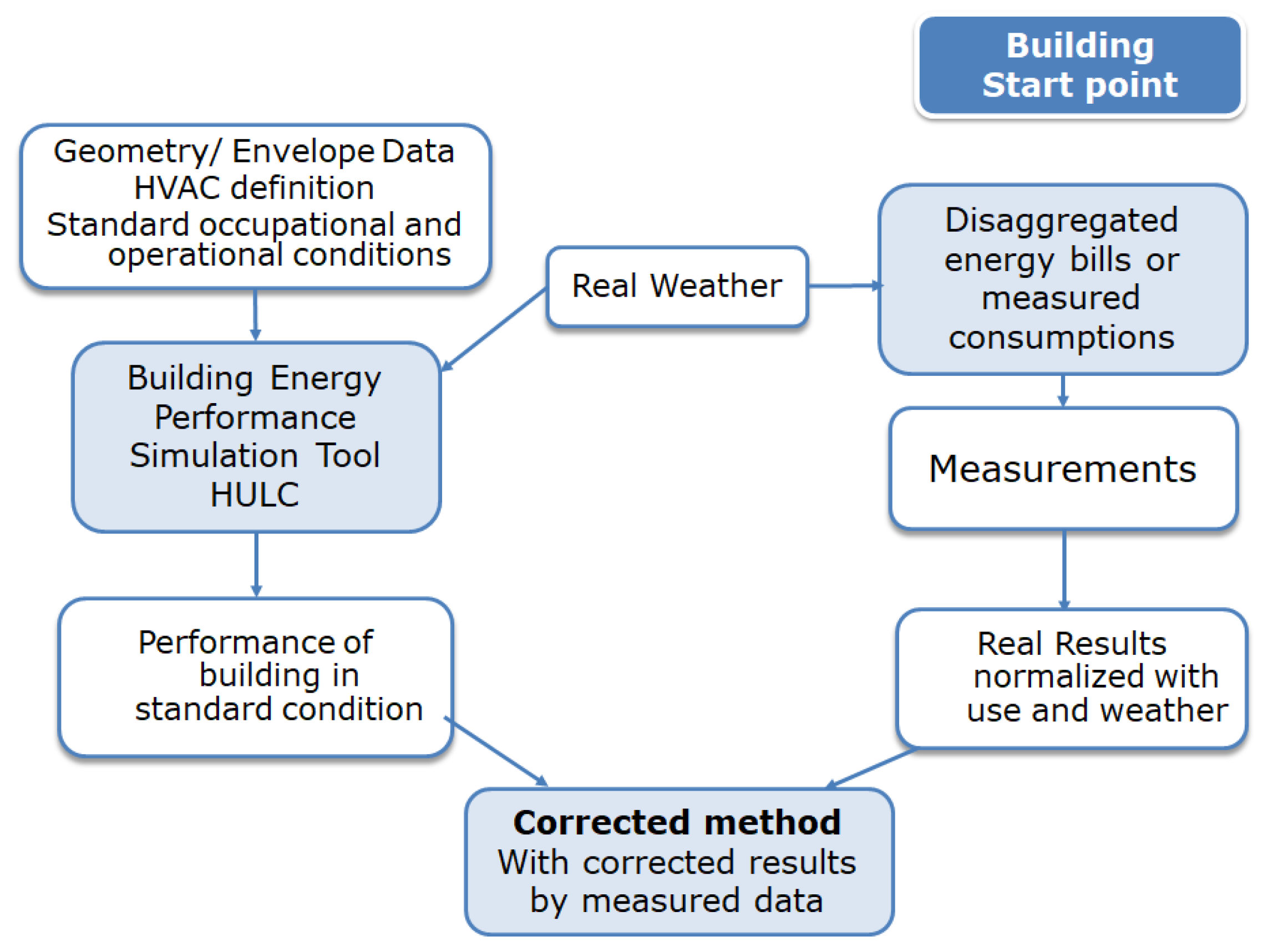
1.4. Correction of Energy Simulation Results Using Energy Bills

A very frequent topic in the literature is the difference that appears between measured consumptions or temperatures in buildings and the results of simulations. These differences are mainly due to the assumptions from the calculation engine itself and the data input errors. Correction is understood to be the process that takes place once the building is defined with the most likely estimations, establishing a way to interpret the results from the simulation tool by comparing them with the measured variables. Normally, the correction process consists in the search for corrective coefficients of the results obtained from detailed simulation tools. These coefficients are defined by the comparison between the estimation of simulation tools and measurements of the building.
Confusing correction with calibration commonly occurs, the latter referring to the modification of inputs, definition parameters and calculation hypotheses so that the results from the simulation are comparable to the measured values. The author of a study [20] gives a practical perspective of the calibration procedures. This paper justifies the need for calibrated tools and for the cost analysis that must be performed, balancing what is gained by the calibration with what has to be spent on monitoring/work to do so. In addition, the authors make an important reflection: A detailed tool consists of thousands of empirical or analytical models that have hypotheses or simplifications to make them operational. The authors [20] emphasize that to calibrate a tool correctly, it is necessary to be its sole administrator, in charge of both of the input parameters and the hypotheses or simplifications. In other words, to calibrate a tool correctly, it is necessary to be its owner and understand even the smallest components of the simulation.
Many studies have been published [24,76,77,78,79] reporting the need to calibrate the buildings’ energy simulation tools, even proposing complex methods oriented to enable the process. However, they all start with highly detailed models of the buildings and involve large-scale monitoring of the buildings over long periods of time. This is an obstacle for existing buildings [80], where there is great difficulty in obtaining data about the construction of the buildings, their operation or even to obtain data from monitorization campaigns performed over long periods of time. The reality with existing buildings, as stated on a previous review [80], is that the information available usually consists on the geometry, little information about its use and the energy audits for the properties.
However, it is usually possible to obtain energy bills from existing buildings over an extended period of time. These invoices can either be itemized thanks to the existence of sub-metering in the building or can be broken down. Whatever the option, these data represent the cornerstone of energy service companies and the owners of buildings. These companies can be drivers of energy efficiency at the consumer level [81], but they need to face the many obstacles existing today [82]. In other hand, José L. et al. [83] show how important is to take into account real consumption in decision-making methodologies.
Thus, it is necessary for energy characterization procedures to be adapted (correction) to available information with sufficient accuracy. In addition, these simplified procedures can guarantee high levels of accuracy with simple input. However, above all, these models can be corrected more easily using real consumption data.

1.5. Aims

The main objective of this study is to develop a simplified method that provides support to procedures that assess, in economic and energy terms, measures to improve the energy efficiency of buildings. The methodologies innovative aspect is the sum of three advantages when it is compared with the existing methods:
  • The method proposed takes into account the lack of information available from existing buildings. For this reason, a vastly reduced amount of data is required to run the monthly baseline model.
  • The functional dependence of the baseline model proposed on the energy parameters of the building makes it possible to analyze the energetic and economic impact of the passive measures combinations on the building, active measures in the buildings’ heating and cooling systems, and even on the incorporation of renewable energy.
  • The results from running the baseline model can be corrected using measured values, which eradicates the differences between the estimated values and real ones caused by the lack of information available regarding the buildings.
The method is validated by comparing its results with those from a detailed simulation tool and then corrected using experimental values in order to reveal its strengths. Finally, the actual application is developed to define comprehensive energy rehabilitation projects in residential areas at risk of energy poverty.
The methodology developed aims to advance towards a sustainable future and to increase the positive effects of energy improvements from the last few decades, given that the implementation of the traditional approaches has proven to be weak, allowing the increase of the energy demands and lacking a clear alternative to address the uncertainties of deficient energy-saving plans.
The existing need to design ground-breaking, understandable, simple, and accurate methodologies to promote the improvement of existing buildings in terms of energy performance, motivates the valorization and development of this work. The presented approach shows an elevated potential, for residents as well as private and public entities, to define optimal and economically feasible energy rehabilitation plans. The implementation of the method could be reinforced by energy policies in the near future, although it would be primarily driven by the tangible benefits achieved in terms of energy and economic savings.

2. Methodology

The proposed methodology aims to obtain simplified models on a monthly basis [29] that can be corrected using experimental data from air pressure testing [84,85], experimental values of the UA (it means U-value by the exposed area of the building) of the building [86,87], or using electricity consumption from bills [88,89]. The model allows decisions to be made regarding the best alternatives for renovating buildings.
This simplified model was deduced from the reduction of a higher-order model of thermal demand calculation (detailed model) of a simulation tool (step 1 in Figure 1). This means that the parameters of the simplified procedure may be obtained by simulating the baseline case (without improvements) in a detailed tool. There are many valid tools, such as Energyplus [52] or TRNSYS [53]. Finally, using the measured consumption data and the actual climate, the correction law of the previous simplified model was obtained. Besides, certain simplified procedures require being an advanced user or the owner of detailed building simulation tools. However, the most conventional building energy performance tools propose methodologies using detailed software simulations. As the results of the simulation tool are used as a starting point of the sequential procedure to correct them with the measured data, Figure 1 below shows the basic principles of the methodology:

2.1. Scheme of Execution

The diagram from Figure 2 provides an outline of the implemented methodology:
The main steps of the methodology (see Figure 2) can be summarized as:
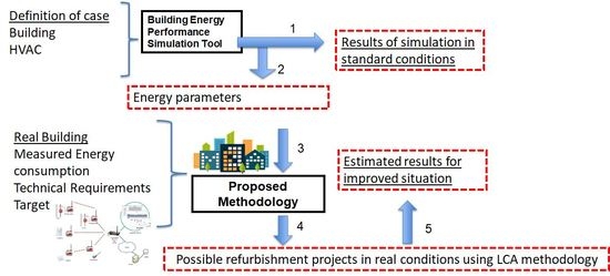
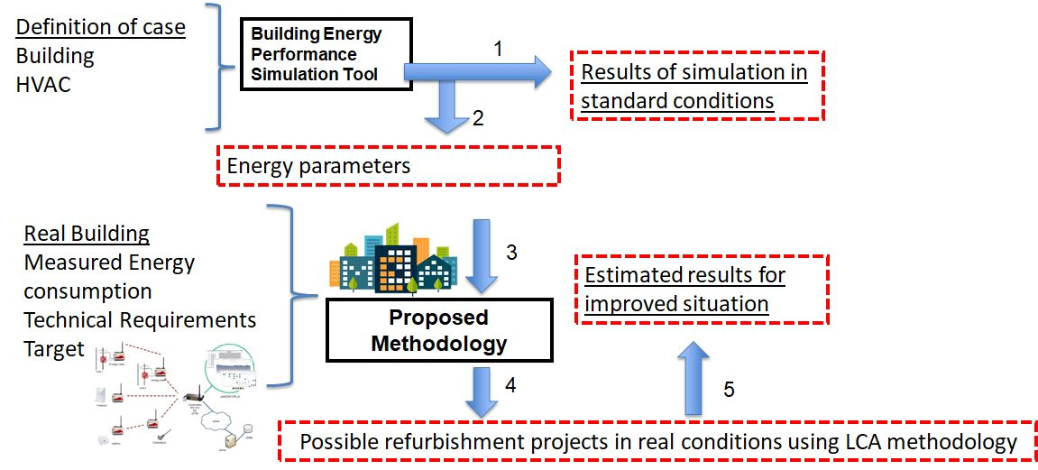
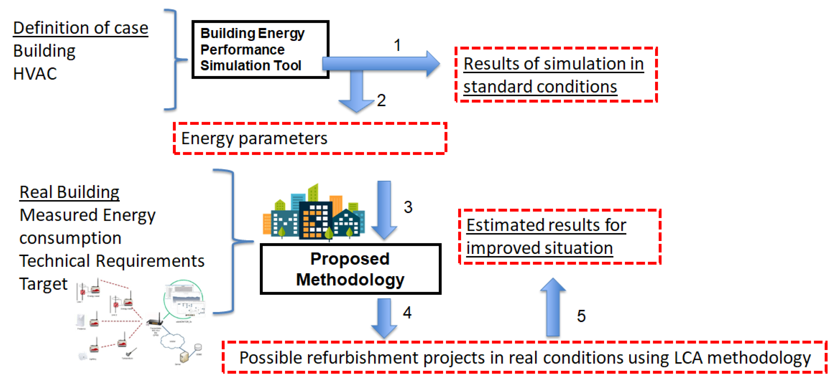
  • Step 1: First, it is necessary to obtain the buildings’ basic parameters. For this first step, it is possible to define a case study using any building energy performance simulation tool (BEP tool). The methodology establishes the need to input the characteristic parameters from buildings’ energy performance and systems, which can be calculated using any computerized tool, such as TRNSYS [55] or EnergyPus [54]. The energy parameters obtained in this paper include seasonal performance factors, thermal envelope characteristics, and shading factors. To obtain these parameters, the authors have used the detailed Unified LIDER-CALENER software tool (HULC), which is the official building energy certification tool in Spain [90], developed by the authors (for more details view Section 3.4). There are quite a few publications developing its use [65,74,91,92,93,94,95,96], which allowed certain modifications to be made in order to carry out the validation of the proposed methodology. It is important to highlight that previous simulations using a BEP tool have not been detailed because it will be used as a starting point for the methodology, subsequently calibrating the results using the energy consumption measured in the actual buildings.
  • Step 2: Second, it is required to extract the results from the simulation of Step 1. Results from detailed tools allow to obtain the starting point to understand the thermal behavior of the building and its systems. A diagnostic procedure is the key to choosing possible energy savings actions. These results are the most conventional, and they are provided for the majority of the tools cited. Therefore, it defines a simplified model using parameters resulting from the simulation.
  • Step 3: Third, the methodology requires real energy consumption, as well as the matching climate data. This information is the input to obtain the corrected simplified model. Then, it is needed to collect the actual consumptions of the studied building (using energy bills for example).
  • Step 4: Finally, it is possible to analyze all energy-efficiency plans and their combination in a short time. This is possible thanks to the use of the simplified methodology (defined using energy parameters from steps 1 + 2 and calibrated using the energy consumption from the third step, as described below in Section 2.2). This is so because the methodology allows to define energy savings measures through the modification of the parameters.
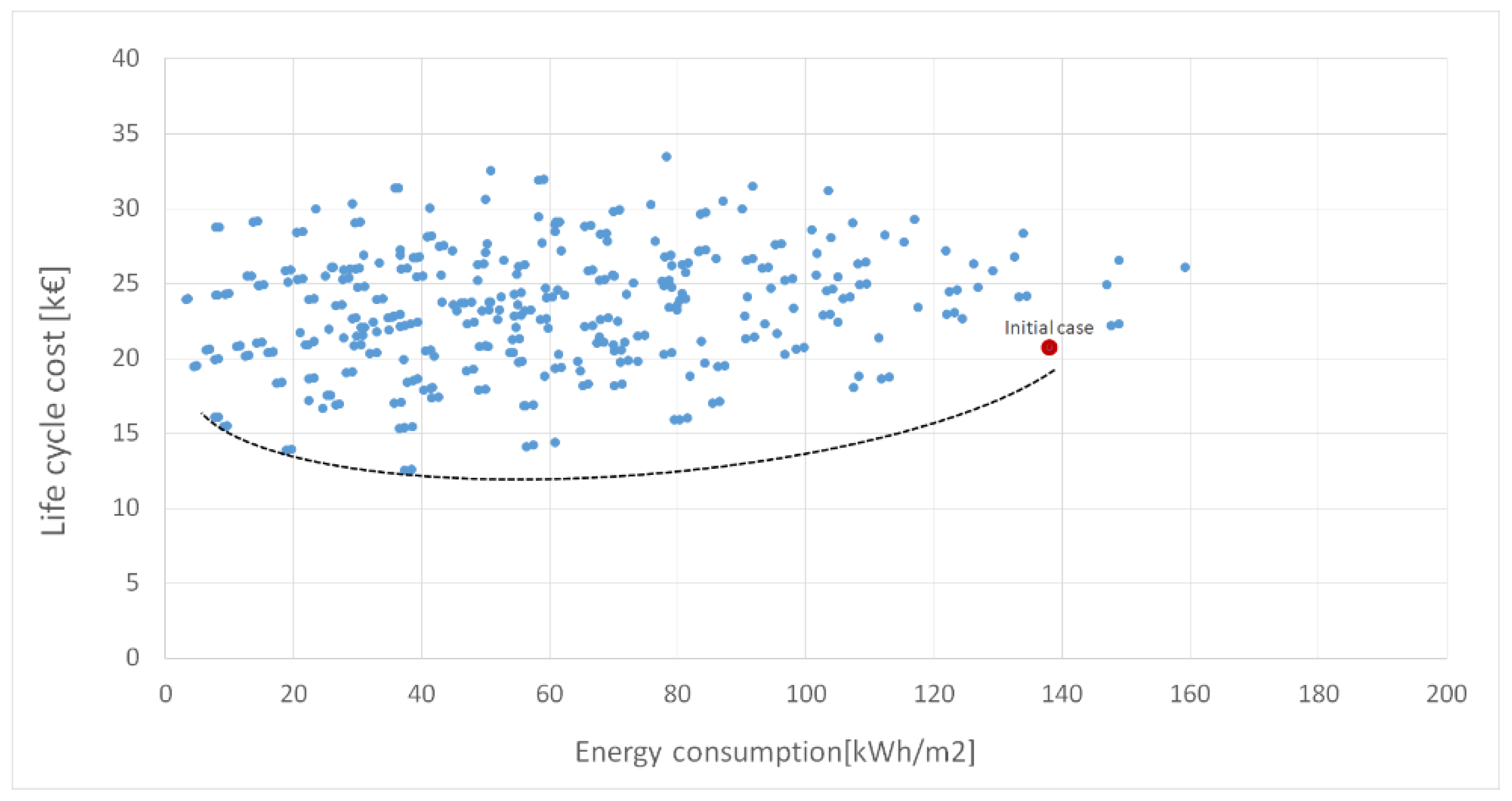
  • Step 5: It uses a life cycle energy assessment to obtain the most interesting rehabilitation project.
The proposals’ core is the simplified model to characterize the real energy consumption (heating and cooling) in buildings. Because, this model allows making detailed parametric studies of the buildings in a simple and quick way, but with estimates closer to the reality of the buildings than using conventional simulation tools. The next section explains the basis of this model.

2.2. Model Assumptions

The simplified model presents the following assumptions:
  • The model has been developed in steady-state.
  • Dynamic effects like thermal mass (inertia) are taken into account by correcting coefficients, and transient effects are considered by correcting coefficients and the utilization factor η .
  • By simulating the baseline case in the detailed tool, the duration of the heating and cooling seasons is set. Consequently, months are not considered with simultaneous consumption for heating and cooling. This hypothesis is on the safe side as the assessment of measures of improvement will only be made in critical months, setting aside intermediate months.
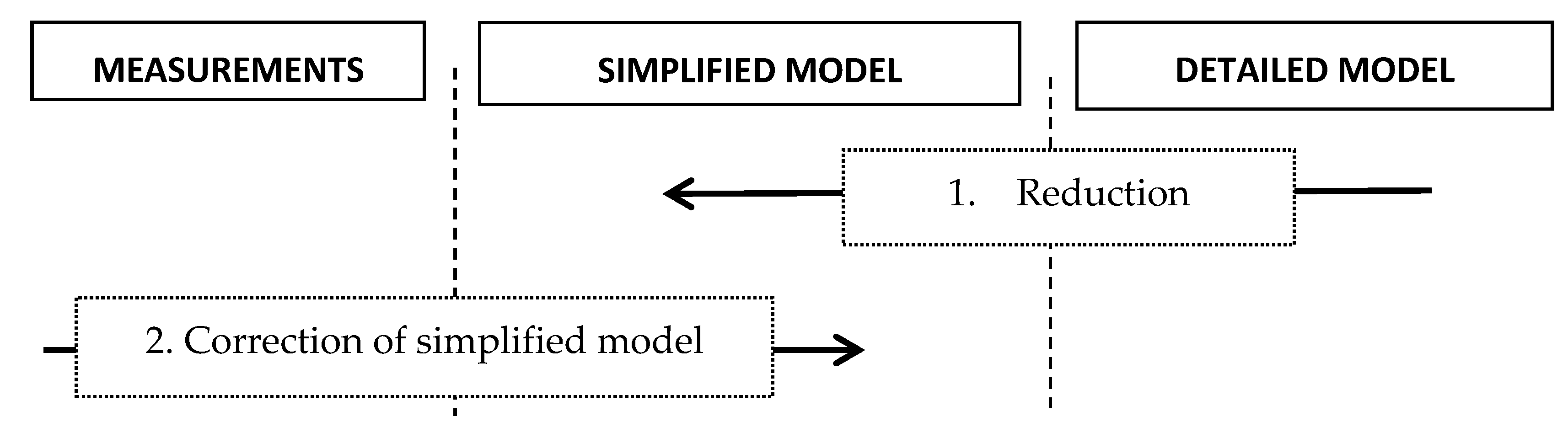
  • The detailed tool is connected to the simplified procedure using the simulation results and the characteristic energy parameters of the building and its systems. The case in the detailed tool must have the real geometry of the building and the best possible definition of the remaining elements. This definition will later correct using the simplified method. This correction adapts the value of the energy flows to the real measurements.
  • The simplified model proposes an innovative way to analyze HVAC (heat ventilation air conditioning) and renewable systems.

2.3. Model Fundamentals

The simplified model matches the modeling methodology established by the standard ISO 52016-1:2017 [28] for estimating energy needs for heating and cooling. However, this study has added several modifications and innovations to the previously cited regulations in order to improve its capabilities:
  • The procedure allows the correction of the results obtained by the BEPS (building energy performance simulation) detailed tool, and even its calibration.
  • The procedure is valid for residential and tertiary buildings.
  • The aim is to characterize the energy demands of the building and the air treatment and energy production systems.
  • A simplified model is established on a monthly basis, governed by the principles for calculating the ideal thermal demand set out in standard ISO 52016-1:2017 [28], adding a correction between the calculated ideal demand and the real one, and then solutions are provided for heating and cooling systems.
  • The procedure can be integrated into ESCO (energy service company) contracts like the baseline energy for the building.
Therefore, model parameters such as shading calculations, radiant distribution, and performance of thermal envelope components, etc., were adopted from this standard.
The formula for building heating and cooling consumption CHVAC-i (kWh) for month i is the following:
C H V A C i = C P H i + C P C i
Equation (1) is the sum of consumptions for month i space heating C P H i (kWh, see Equation (2)) and space cooling C P C i (kWh, see Equation (3)). However, as stated above (Equation (1)), only heating and cooling consumption exists for month i, simultaneous consumption not being considered.
Equation (1) can be generalized to include the contribution of systems based on renewable energy since Equations (2) and (3):
C P H i = D H E A T i · R D H η P H ¯   · ( 1   C R H ) + D H E A T i · R D H η P H R E N ¯   · ( C R H )
C P C i = D C O L D i · R D C η P F ¯   · ( 1   C R C ) + D C O L D i · R D C η P C R E N ¯   · ( C R C )
The ratios of demands R D H   (see Equation (2)) and R D C (see Equation (3)) are parameters for getting energy demand in heating and cooling system through ideal demand of the space. This new demand takes into account the losses, latent energy and the effect of the measures on the secondary system etc. In residential buildings this parameter is assumed to take the value of 1. At the same time, Equations (2) and (3) show the contribution of renewable energy in order to satisfy the heating and cooling demands (   C R H and C R C ). Finally, the seasonal production performance (heating η P H ¯ and cooling η P C ¯ ). It can see that methodology takes into account renewable energy production by using another seasonal production performance for this system (heating η P H R E N ¯   and cooling η P C R E N ¯ ). Besides, they are broken down into two so that it is capable of considering, for the renewable energy system, a different heating production performance.
First, the ideal demand, which maintains set point temperatures for heating and cooling ( D H E A T i (Equation (2)) and D C O L D i (Equation (3)) respectively in kWh), is modelled according to the climate, geometry and construction of the building with Equations (4) and (5).
D H E A T = a H · Q L O S S H b H · η H · [ Q G A I N S U N + Q G A I N I N T ]
D C O L D = b C · [ Q G A I N S U N + Q G A I N I N T ] a C · η R E F · [ Q L O S S C ]
On this basis, energy demands are a function of: The heat losses through the thermal envelope of the building and its infiltrations, Q L O S S H (see Equation (6)) and Q L O S S C   (see Equation (10)) respectively, solar gains, Q G A I N S U N (see Equation (7)) and internal gains due to occupancy, equipment and lighting (use of the building),   Q G A I N I N T (see Equation (8)).
It is worth mentioning that the effect of the buildings’ inertia is linked to the utilization factors η H   (Equation (4)) and η C (Equation (5)). The guidelines from the standard [29] and some publications that analyze this term [30] were used to formulate them. The utilization factors η H and η C mainly depend on the building time constant and the ratio of gains and losses. These utilization factors indicate the percentage of gain used to reduce the energy demand for heating or, in the case of cooling, the flow of losses used to reduce the demands for cooling. However, after a review of the literature focusing on this parameter, it was noted that there is a trend, represented by [97], in which this parameter is a function of the characteristics of the building (UA (W/K) and its thermal capacity (J/kgK)). Although there are also studies [30] in which the utilization factor is studied in detail for the heating season, these studies propose taking the results of the standard [98] but identifying the value of the building time constant by means of simulation.
In addition, the coefficients a H , b H , a C   and b C (Equations (4) and (5)) are adjustment parameters. These coefficients were used to modify the estimation of the simplified model. This modification aimed to correct the model using results from the detailed tool. For this reason, these coefficients made it possible to reduce the detailed model into a simplified one.
Heat fluxes, which appear in Equations (4) and (5), depend on the characteristic parameters of the building, climate variables, occupancy conditions and use of the building. Therefore, it was necessary to know how these fluxes could be modeled. For example, heat losses through the thermal envelope and infiltrations are shown in Equation (6).
Q L O S S H = ρ · C p · V · A C H e q · 24 · D D 20 3600 + U M · A T · 24 · D D 20 3600
where ρ is the air density (kg/m3), C p specific heat of air (kJ/kg·K), V air volume of building ( m 3 ),   D D 20 degree-day 20 (°C·day) which refers to month, and U M the transmittance value of the transfer surface A T taken into account. A C H e q (h-1) is air change per hour due to ventilation and infiltration. Thus, U M and A C H e q are two of the buildings’ characteristic parameters that could be estimated using detailed simulation or real data.
Heat gains can be divided into two: Solar and internal gains. Solar gains are defined in Equation (7).
Q G A I N S S U N = E S A i · I S o u t h
where E S A i (m2) is the equivalent south area per month and unit area of glazing, and I S o u t h (kWh/m2) is the incident solar radiation (direct and diffuse) on the south-facing elevation. It is important to comment that Q GAINS SUN should be in function of the north for buildings in the southern hemisphere ( E S A i would be equivalent north area per month and unit area of glazing, and I S o u t h would be is the incident solar radiation (direct and diffuse) on the south-facing elevation). The ESA parameter is considered quasi-static as it characterizes the effect of solar gains on heating and cooling consumption and is highly dependent on the solar radiation falling on the building envelope, which is absorbed and enters the building through its semi-transparent elements. Consequently, the ESA parameter changes every month. The definition of this parameter was adopted from [99]. This formula makes it possible to assess the effect of solar control by reducing the ESA parameter during cooling months.
Finally, energy gains due to internal sources within the building (Equation (8)) can be characterized from the length of the calculation period ( t ) and the parameter ϕ (kWh/m2), calculated using values for occupancy, lighting and appliances in the building.
Q G A I N S I = ϕ · t
The only losses considered in the cooling months are those due to night-time ventilation (Equation (9)). This is so because the effect of transmission through the building envelope and infiltrations was considered to be zero on a monthly basis because a positive value is taken as a gain at certain times of the day and negative values as losses during others. Night-time cooling is also the most common measure taken for reducing energy demands for cooling. This heat flow is modeled (Equation (9)) as air change per hour during night hours ACH NIGHT , taking 25 °C to be the reference daytime temperature D D 25 N I G H T (°C·day).
Q L O S S C = A C H N I G H T · ρ · C P · V · D D 25 N I G H T · 24 / 1000
All the necessary parameters are usually calculated in any building energy performance tool. The values of these parameters to evaluate energy savings plans were obtained from several references, such as [11,74,83,100]. This last option enhances the versatility of the model as a simplified tool. Furthermore, it is important to highlight that the simulation tool offers results with open access with regard to each of the parameters utilized here, which are the most commonly used in procedures for the thermal diagnosis of buildings, as shown in scientific publications such as [101] and the reports of the EPBD [102].

2.4. Correction of Simplified Method Using Measured Data

A case study was developed to analyze the thermal behavior of buildings in detail. This means that a model with an accurate estimation of the geometry, materials, orientation, and exposed surfaces of ceilings, walls, and floors is available. The building model was developed using the detailed Unified LIDER-CALENER software. Figure 3 reveals the procedure to link energy bills and the simulation results. It should also be emphasized that comparison between the simulation tool and the energy bills was made using the simplified methodology (for more information see Figure 1).
The left side of Figure 3 shows how the case was defined in the HULC simulation tool and simulated using matching climate conditions. This simulation produced results for the energy demand of the building under standard conditions [54]. The right side of Figure 3 shows the true consumption data obtained from itemized bills, data which are then compared with the data estimated using the simulation tool. This comparison enabled the case study to be analyzed and the optimal correction of the results to be achieved. This correction is valid for the whole season since coefficients are constant, varying for heating and cooling.
Likewise, the energy reduction from the detailed simulation to the simplified model can be performed with a simulation using typical meteorological years, for example, weather files proposed by EnergyPlus [54], if no hourly measures for real weather are available. This would not be a problem because the weather is an independent variable in the simplified method. Thus, at a minimum level, the method can be used when only mean monthly outdoor temperature values and global horizontal irradiation values are available.
The real consumption for heating C H i (kWh/m2) and cooling C C i (kWh/m2) are comparable to the estimations from Equations (2) and (3), respectively, when they are executed using real climatic conditions. With that in mind, the correction procedure involves the comparison of estimations obtained using the monthly simplified model identified with experimental data and the estimation obtained by means of the detailed simulation. Using a conventional optimization procedure, this procedure allows the extraction of the monthly correction factors ( F C H 1 and F C H 2 for heating and F C C 1 and F C C 2 for cooling) for the model to be obtained from the simulations. This results in the following corrections:
C H i = F C H 1 · C P H i + F C H 2
C C i = F C C 1 · C P C i + F C C 2
It should be clear that the correction is made in an indirect way, through a monthly simplified model obtained from reduced knowledge from the detailed model, which is the one used by the tool. Furthermore, the simplified model with measured data (Equations (10) and (11)) has value in itself, either as a baseline for the verification of savings or for error detection related to energy management, provided that it is identified with measured heating or cooling consumption data during a useful reference period.
When energy bills from existing buildings are available, the real consumption data can be compared to those obtained from the simplified model. In some cases, this comparison can highlight great differences, a phenomenon known as the performance gap between an energy model for buildings and real measurements.
In other words, these differences are because all simulation software has to deal with uncertainties, and it is, therefore, necessary to assume a certain number of hypotheses, mainly regarding climatic data, conditioned area and user behavior.
Table 1 summarizes reasons for the performance gap through the analysis of real conditions and the assumptions and hypothesis used by the simulation software.
The adjustment methodology was developed assuming that the main differences when comparing simulation results with real consumptions are due to weather data, real conditioned area and user behavior. As shown in Equations (10) and (11), the effects of climate are neutralized by allowing the calculations to be made using matching meteorological conditions. Furthermore, differences between the real and simulated conditioned area and user behavior were corrected through correction factors in Equations (10) and (11).

3. Validation of the Simplified Methodology
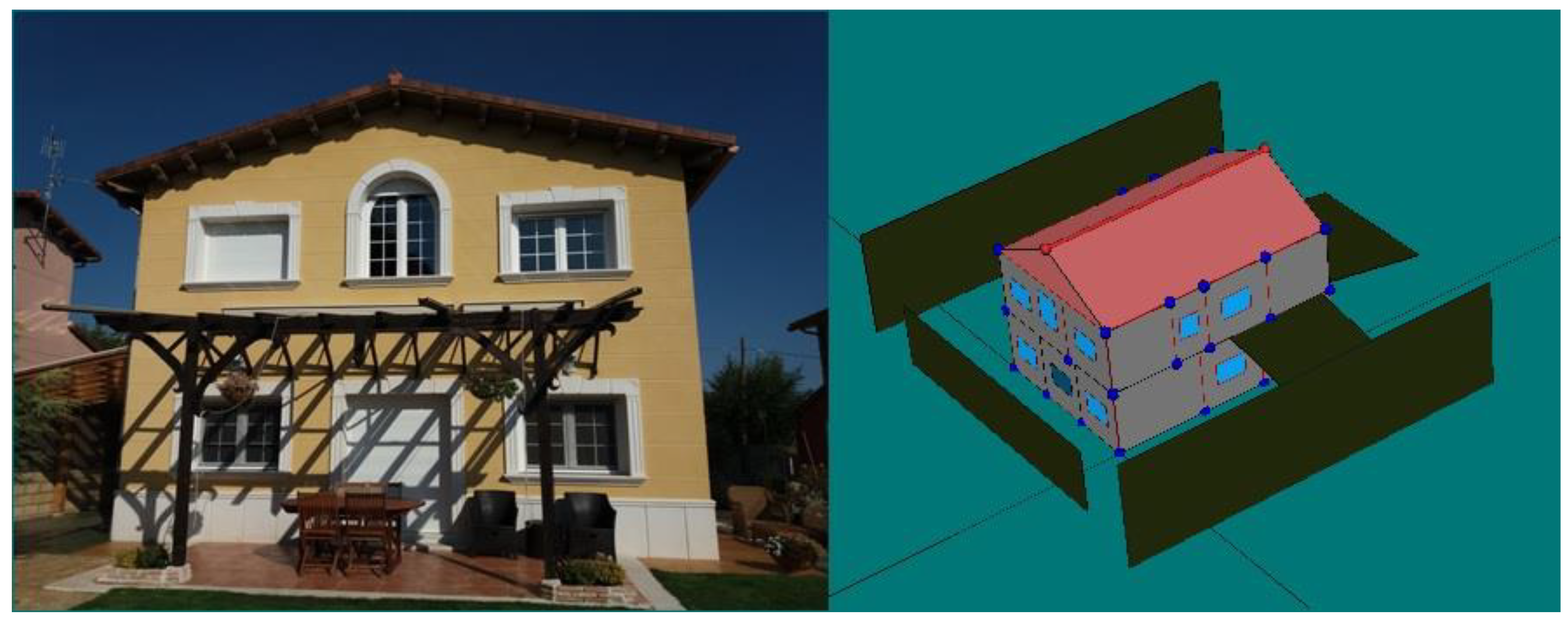
In this section, the procedure is tested on a real dwelling. First, the procedure is validated by comparing the estimated savings generated by a detailed simulation tool and the estimates using the simplified method (robustness of the simplified model defined using a detailed simulation tool). Finally, the validity of its use is tested using the measured consumption data available from the dwelling. This demonstrates how the procedure provides a solution to the differences between simulated and measured values, for both new and existing buildings.
The first step is to emphasize the quality of the envelope in order to get highly efficient buildings with low energy needs. The most common way to achieve this is through high levels of insulation in opaque elements and high-quality windows. This point compares the results of these actions using the simplified and detailed models. In addition, night ventilation (during cooling season) is analyzed too.
The main objective is to demonstrate the capacity of the model to study energy-saving measures and how it can be adapted according to the quality of the data available.

3.1. Case Study

The case study relates to a detached house located in Madrid (see Figure 4). All the as-built information and energy bills for the house for the years 2016, 2017, and 2018 are available. These energy bills are used in Section 3.4 for correcting the simplified methodology. However, in Section 2.4, there is a comparison between the simplified and detailed methodology.
Table 2 and Table 3 show the main parameters of the building under study. The process of obtaining these parameters is the reduction process detailed in Section 2 (see Figure 2).

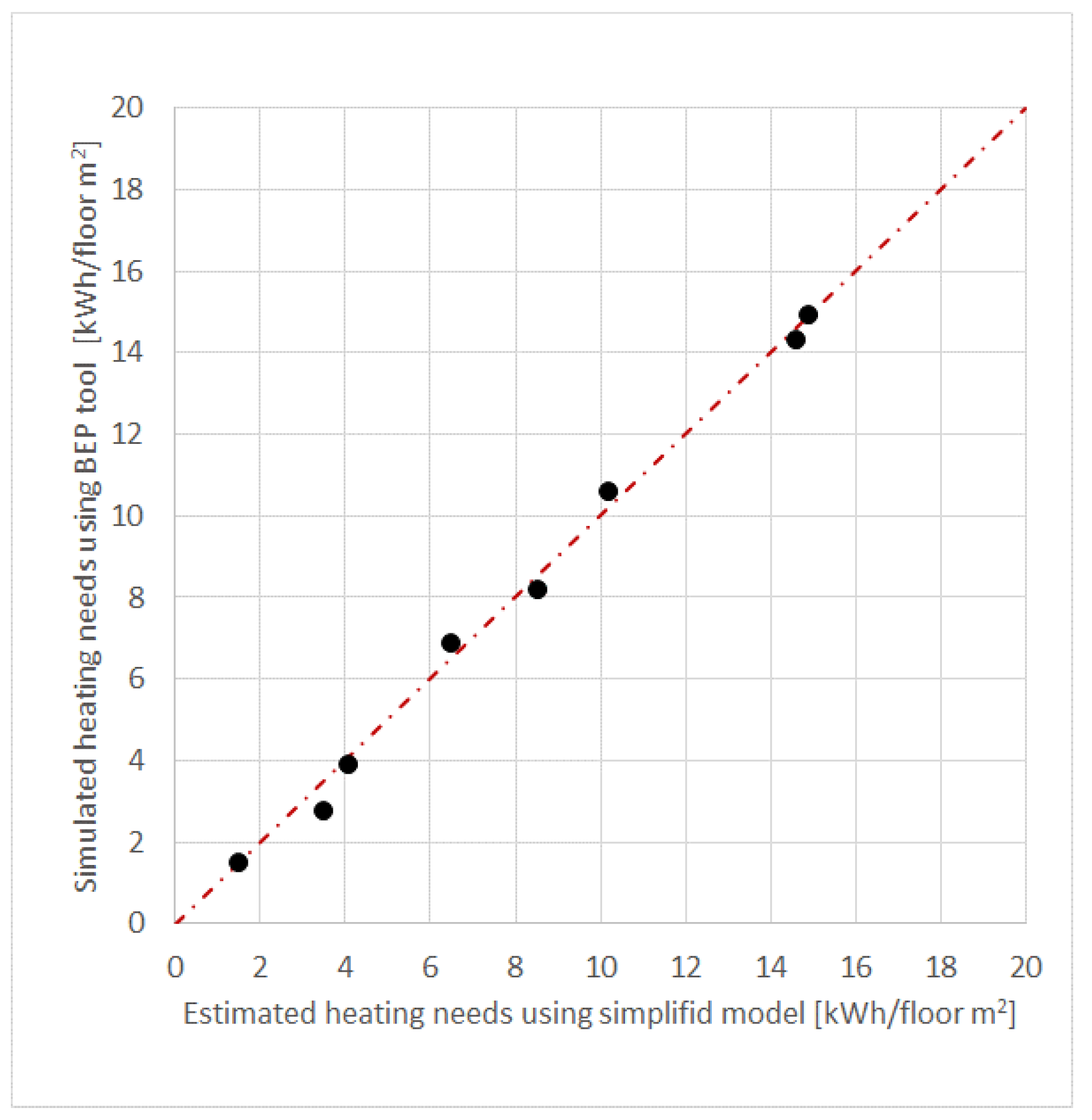
3.2. Define the Simplified Model (Reduction of Detailed Model)

For the building described, the model is then identified based on the results of a detailed procedure.

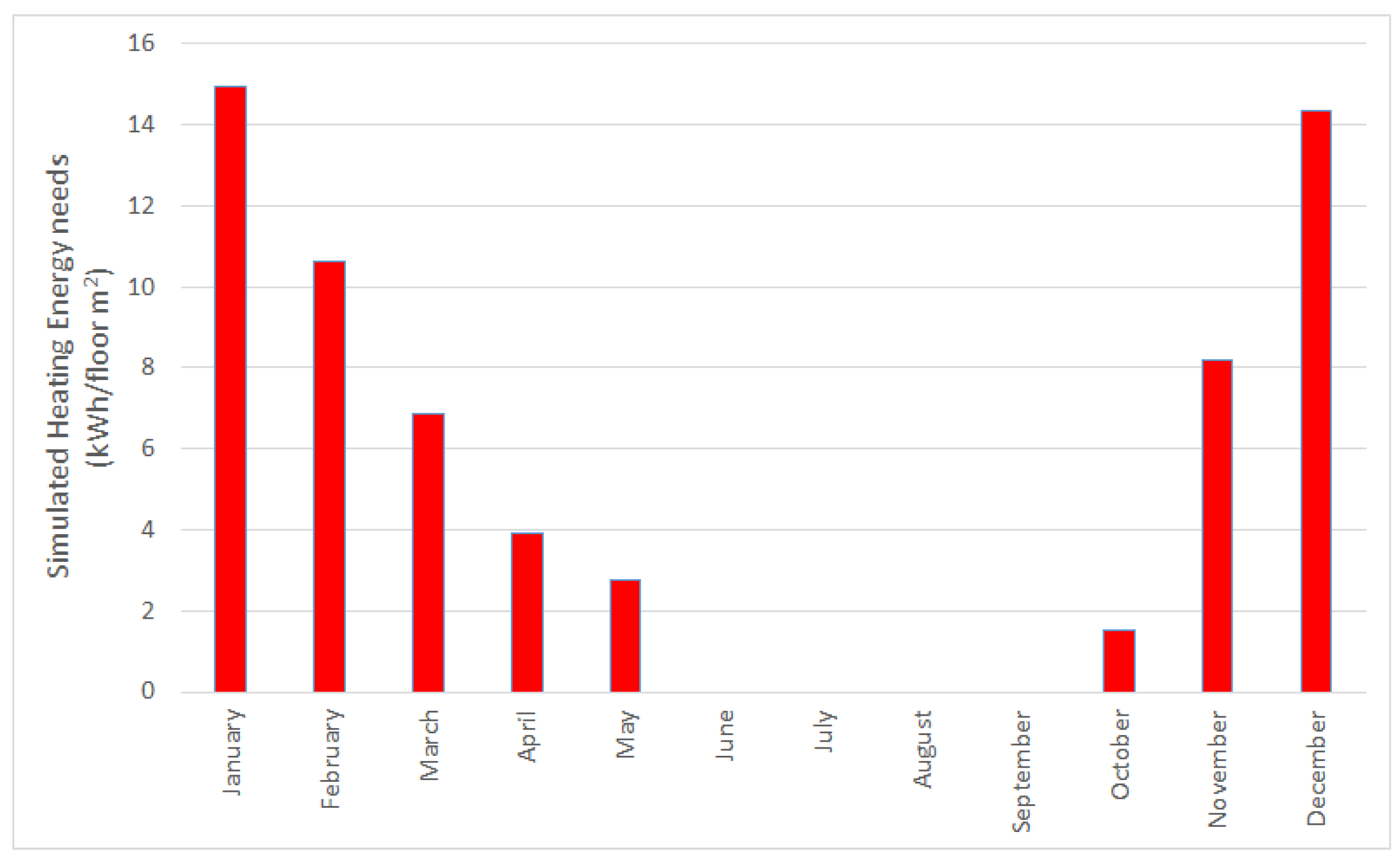
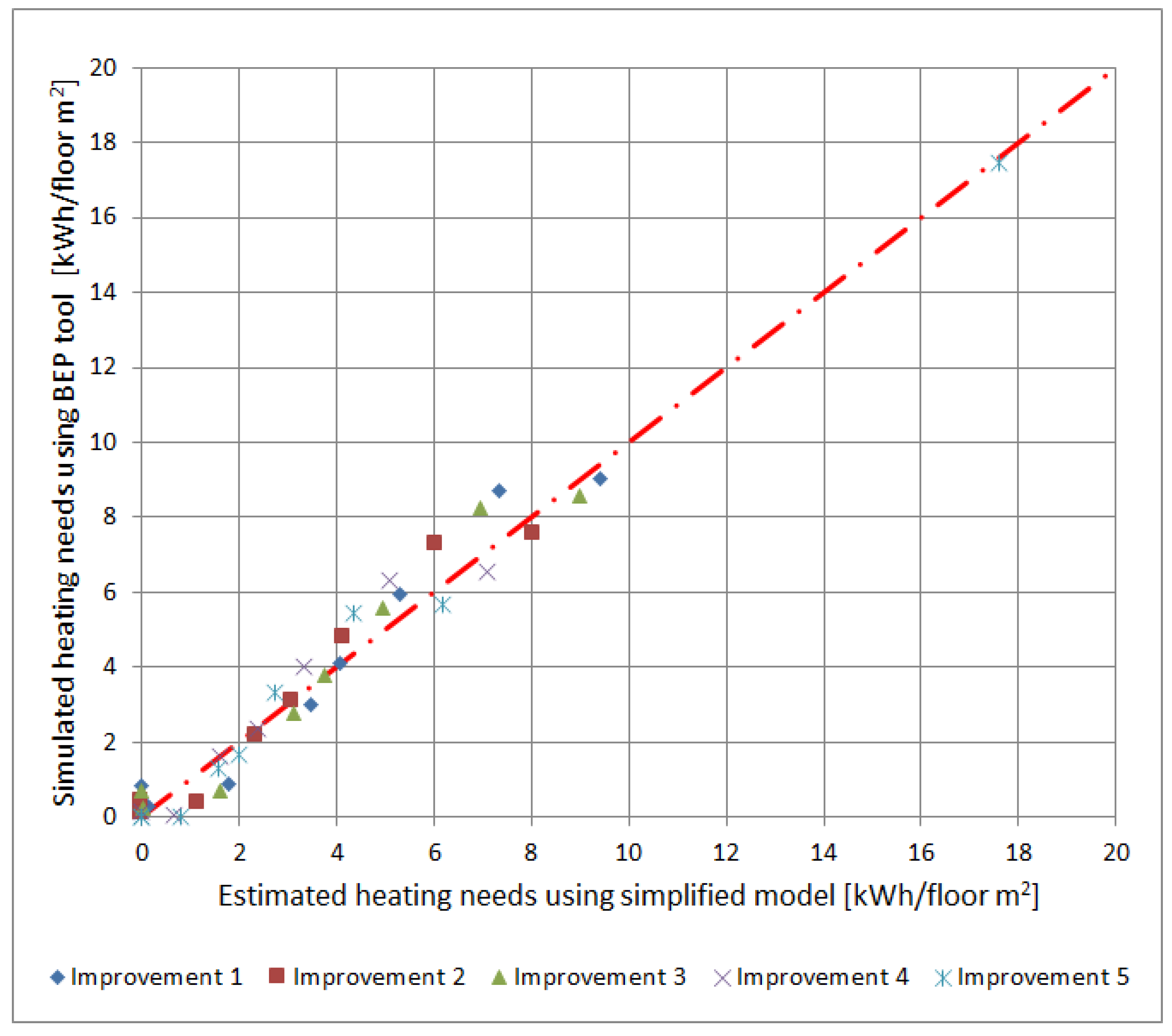
3.2.1. Heating Period

The results of the heating need to be obtained by means of a detailed simulation tool shown in Figure 5.
Figure 5 shows that January, February, March, November, and December are the main months when heating is required, and in April, May and October heating is needed during part of the day or on some days. In this case, all the months stated above are taken as heating months, which leads to the added difficulty that the procedure has enough sensitivity to make an acceptable estimate for the coldest month January and some other months like May. The reduction of the detailed model to the simplified heating model (see Equation (4)) was obtained by identifying the value of the coefficients a H = 1.00 and b H = 0.71   to obtain the best fit between both methods on a monthly basis. The results of this adjustment are shown in Figure 6.
Figure 6 compares the values obtained via the simulation of the case in the detailed tool (y-axis) and the estimated values with the proposed model (x-axis). It shows a good fit (average error of 5%, maximum error of 9%, and a correlation coefficient R2 of 0.98) for all months, regardless of the demand for heating. This result is one of the strengths of the method.

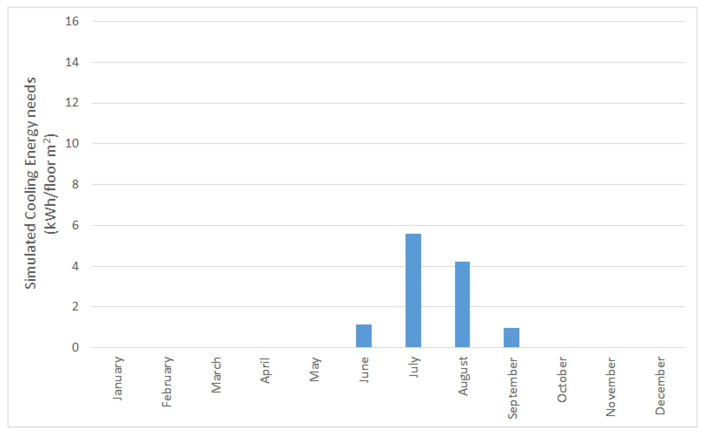
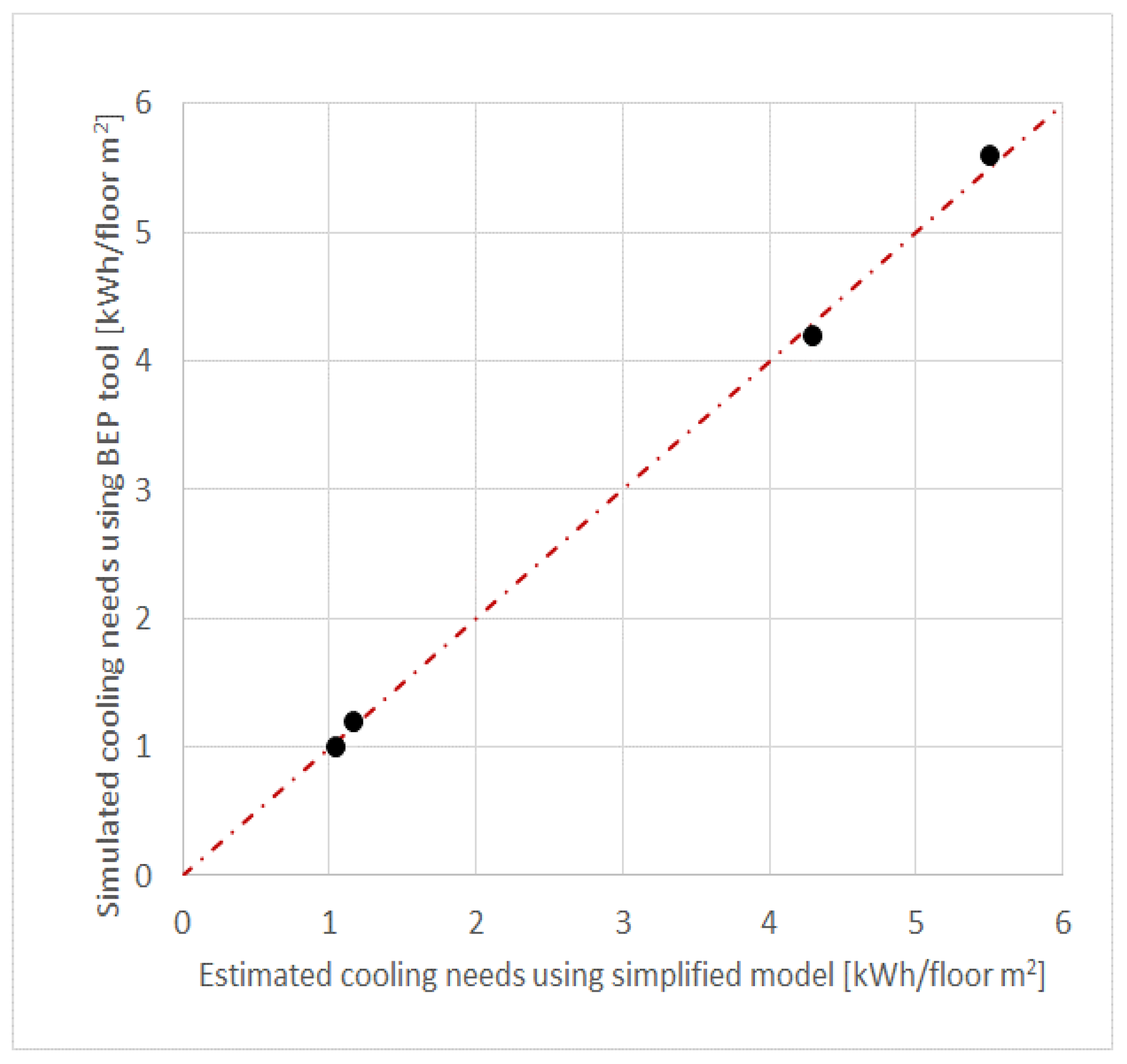
3.2.2. Cooling Period

The case of cooling is more critical since a smaller amount of data is available. The values obtained by the simulation of the case appear in Figure 7.
It works the same as in the case of heating, the simplified model for cooling demand (Equation (5)) is identified by obtaining the value of the coefficients a C = 0.70 and b C = 0.78 . If the simplified model is corrected with the simulation data executed, the results shown in Figure 8 are obtained.
Figure 8 shows a comparison between the corrected simplified model and the detailed model. Then, the simplified model corrected for cooling mode also presents valid results. The maximum error is equal to 7% and the R2 correlation coefficient reaches a value of 0.98.

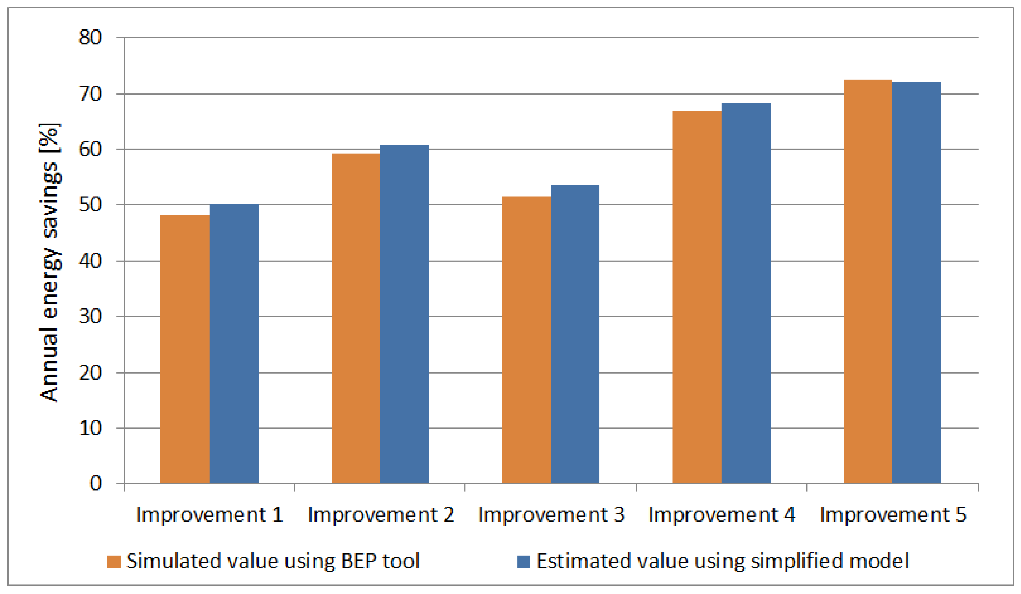
3.3. Energy Savings Evaluation Using a Simulated Scenario

This point highlights the main application of the procedure: The study of energy-saving measures and the savings evaluation. To this effect, simulations are carried out using the simulation tool, and the simplified model is applied. These simulations were carried out by making modifications to the envelope of the building, as described below. The purpose of this section is to identify the monthly model with the data of the baseline situation and forecast the savings that would be produced by modifying the parameters of the model. This forecast is compared with the savings calculated using the detailed procedure.
The measures that were carried out were the improvement of the insulation on the roof, floor, and main façade. At the same time, the combined effect of replacing the glass of the house is analyzed. Table 4 shows in detail the improvements made.
Due to the improvements made and the energy demands of the building, the heating season is considered the most relevant for the study. Figure 9 shows the comparison of the values estimated by the model (correlated demand) and the calculated results (calculated demand) for each of the six previous cases in the heating months mentioned above.
The model from Figure 9, can be considered as valid. However, the estimated annual savings are key in the cost analysis, checked in Figure 10.
The model overestimates the savings, always by below 5% (see Figure 10). This is positive as it means that studies carried out will make estimates that have an acceptable quality. Another important result is the computational cost. When building energy performance tool (HULC) was used, computational cost, for doing alternatives of Table 4, was 34 min and 23 s. Additionally, the same result using the simplified method was 2 min and 10 s (simplified method was implemented in Microsoft Excel before).

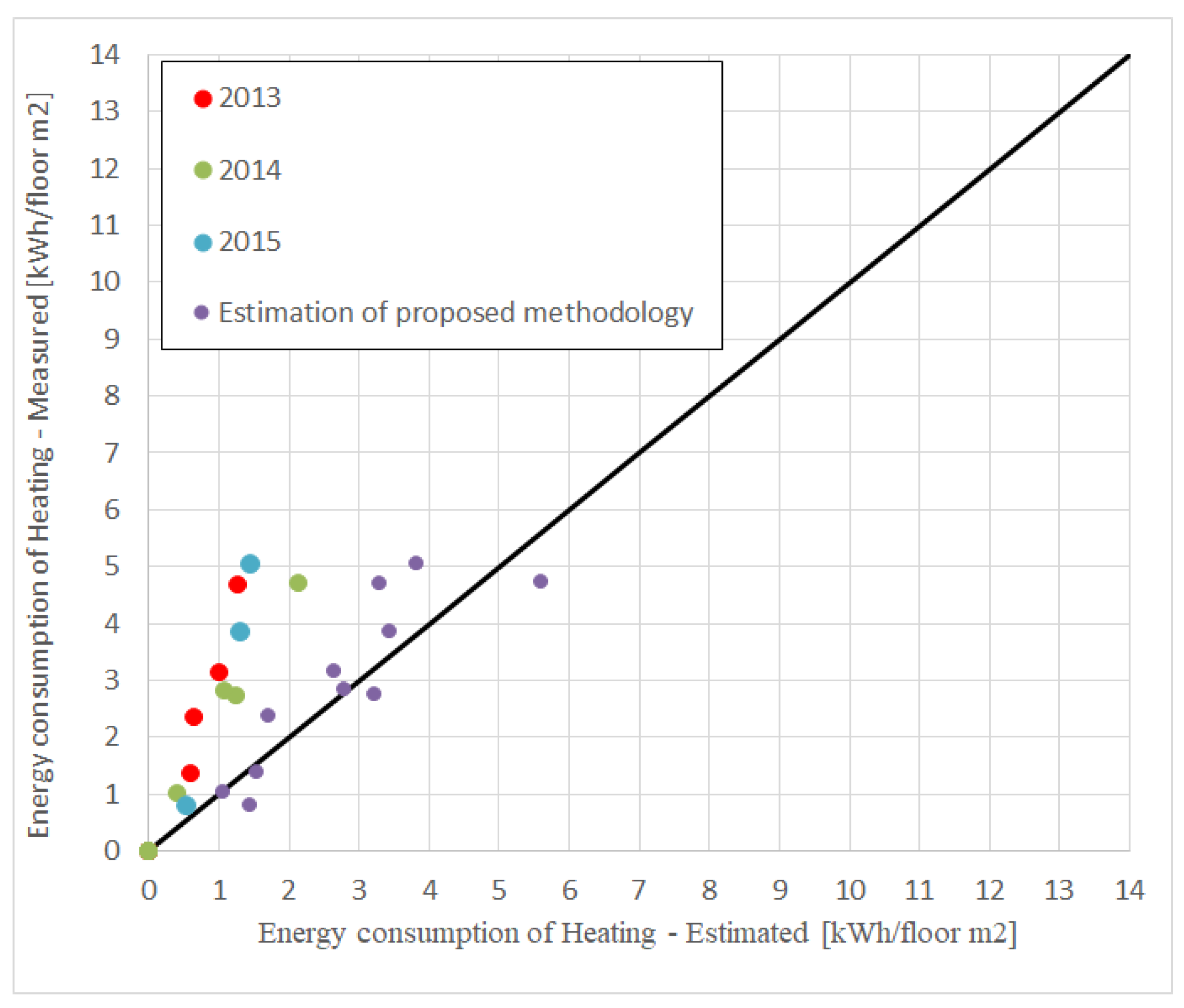
3.4. Importance of Corrected Simplified Model
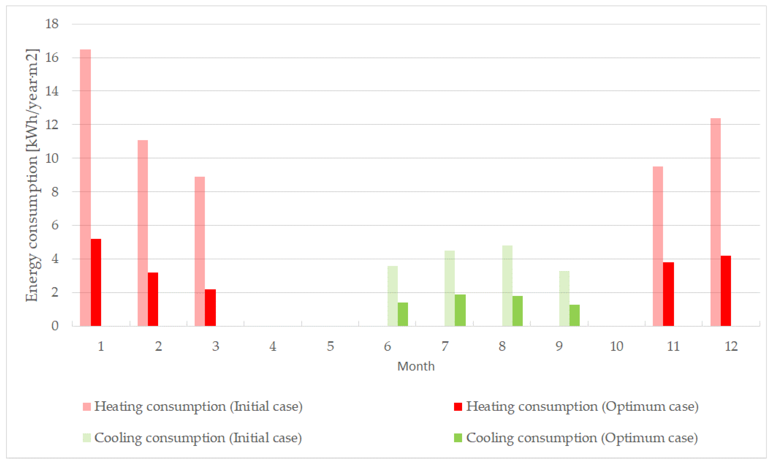
Finally, this section shows how the simplified procedure was corrected using real energy consumption during the heating season (electricity consumption). To this effect, the estimates of consumption made by the model defined in Section 3.2 were compared with the values from the bills in Figure 11 using the actual weather data from 2013, 2014, and 2015. Figure 11 shows the results of the estimate made by the corrected model using energy bills (purple dots).
Figure 11 shows how energy consumption simulated for the heating is always smaller than energy consumption for heating measured. Then, when the simplified methodology was corrected using measured data (purple dots), it was possible to see that estimates were much better. Therefore, this is the proposed way to take into account the real needs of the building in the analysis of future plans.
The need for this correction became clear when improvement measures were analyzed. With this objective in mind and to complement the previous application, particular importance was given to the parameters referring to the heating and cooling systems. First, the performance of the HVAC system was analyzed. The average seasonal coefficient of performance (SCOP) takes a value of 1.13 (measured value using Air-Conditioning, Heating and Refrigeration Institute (AHRI) Standard 210/240 [103]), which lies within the expected range (1.4 to 4.5). On the other hand, the seasonal energy efficiency ratio (SEER) is 1.6 (measured value using AHRI Standard 210/240 [103]) and the expected range is 2.0 to 3.33.
Table 5 shows the three chosen measures and their combinations: Improved insulation of the thermal envelope (acronym INS in Table 5) as a demand improvement (DI) (improvement 4 in Table 4), integration of a high efficiency recovery system in the air conditioning as a secondary system measure REC (SI, improving secondary systems), and a new system for heat production SYS (PI).
Table 5 shows the energy savings (%) in the building using the uncorrected model (Section 3.2) and the corrected model (Section 3.4) using data from energy bills for the most interesting measures from an economic and energetic point of view. Furthermore, the table validates the feasibility of the proposed method for the analysis of measures for improving energy demands as well as the heating and cooling systems.
The first Id from Table 5 shows the combination of these improvements, to reduce the energy consumption in the building by 28.6 kWh/year·m2, which once corrected has a value of 21.0 kWh/year·m2, that is to say, the correction of the savings modifies significantly the internal rate of return (IRR) and payback values calculated.
Finally, it is worth stressing that improving primary systems leads to 40% savings (40% without correction and 32% corrected), as shown in ID 4 from Table 5. ID 1 to 3 show how the combination of measures to the primary system improvements are not relevant because estimated energy savings are similar and the extra cost would not be justified. Therefore, the simplified methodology allows the energy performance of HVAC systems to be assessed, a strength of the methodology. Besides, cases 6 and 7 from Table 5 show that the insulation improvement (INS) and the recovery system (REC) present the same savings (6%). However, the cost of insulation could be between 10 and 20 times higher than the recovery system.

3.5. Application

This section describes how the model was applied in a matter of minutes. The objective was to design a comprehensive rehabilitation project using the developed procedure. Table 6 shows the alternatives studied. Cooling alternatives are named from C0 to C5, some of which are combined with night cooling (C2-5, C3-5, and C2-7). The heating alternatives are named from H0 to H3. All the heating and cooling options were combined with each other.
The different alternatives (see Table 6) refer specifically to the following values:
  • Awnings: On SE and SW facing exteriors, they reduce the solar factor of the windows by up to 50%. This measure is aimed at reducing solar gains in summer.
  • Slats: On SE and SW facing exteriors, reducing the solar factor of the windows to 0.33.
  • Night ventilation: 10, 7 or 5 air changes per hour during the night by means of extractors in the bathrooms.
  • Air permeability of the windows: 9 (high level), 27 (medium level) or 50 (low level) m3/hm2 at 100Pa.
The thermal transmittance of different cases is shown in Table 7. It is the main parameter to define savings measures in the simplified methodology.
The costs of alternatives were estimated by consulting the technical sector. Based on this and following the cost-optimal methodology recommended in the European directive [18], it was possible to compare all the measures and their possible combinations. Figure 12 shows those combinations that generate the Pareto curve for the optimal cost study performed.
Analyzing the results of the different combinations it was possible to identify the optimal improvement. In this project, it proved to be the one using enclosures with transmittance level 3 and windows with a permeability of 9 m3/h m2 to 100 Pa), in addition to awnings for solar control.
Finally, it was possible to obtain the economic estimate at the chosen optimum point, as shown in Table 8. The budget was 14,009 € for the entire house.
The new energy demand of the buildings will be achieved through more efficient heating and cooling equipment. The old low-efficiency ones will be replaced by high-efficiency heat pump equipment with a COP of 3.6 for heating and an EER of 3.2 for cooling. Figure 13 shows a comparison between the initial and the optimum scenario.
The total savings in energy consumption for heating and cooling achieved by the NZEB project after applying these improvements were 69%, as seen in Figure 13. Substantial energy savings are reflected in the building’ indicators, which were reduced from 9.7 kg CO2/m2 year to 2.9 kg CO2/m2 year.

4. Conclusions

A simplified method that provides support for economic and energetic assessment procedures was developed to choose the optimal measures for improving the buildings’ energy efficiency. The method involves a simplified procedure for the buildings’ monthly energy consumption calculation. The following developments are of particular significance:
  • A new simplified model was obtained based on reduced information obtained from a detailed model. However, it is possible to use this methodology without a previous simulation if a database of buildings parameters is defined, for example, performing a previous literature review.
  • The functional dependence on the buildings’ energy parameters, make possible the analysis of the impact from an economic and energetic perspective, the different combinations of passive measures in buildings, active measures related to the heating and cooling systems and even the renewable energy integration.
  • The methodology can be corrected using data from the mean energy consumption. Thus, it is possible to take into account the actual behavior of the buildings in the performed estimates. As shown in Section 3.4, the difference in the estimated savings before and after correction is over 30%, which has significant implications for the economic parameters’ assessment, reducing the estimates’ level of uncertainty.
The methodology was developed taking into account the lack of information available regarding existing buildings. For this reason, the parameters required in the proposed methodology can be obtained from simulations performed by a conventional tool. The verification was performed by comparing the results of this methodology with those from a detailed calculation tool validating the method, with annual errors below 5% in all cases.
The methodologies’ simplicity of use, besides enhancing its potential of application in different cases, enables thousands of alternatives to be analyzed with a low computational cost and without any loss of accuracy. Besides, the time consumed using the simplified model (order of minutes) is 30 times lower than the time consumed by using the BEP tool (order of hours). The methodology is easy to be implemented in web platforms or apps, so the possibility to spread its use is very high.
The emphasis is currently on the achievement of near-zero energy building, since it seems to be an easier task. Particularly, in this case, changing from detailed simulation tools to more simplified procedures may allow economic and energetic studies on a larger scale to assess distributed generation, storage and allow the development of demand-side management strategies.
It is important to highlight that the development of the simplified model involved massive simulations with a detailed calculation tool. As a result of these simulations, different formulation alternatives were ruled out, for example in the case of night cooling or air ventilation systems. From these discarded tests, it was concluded that the current proposal is the most robust to guarantee the reliability of the physical information to be characterized, an important point to ensure the validation of the results before entering different input parameters.
Finally, it is worth to stress on the use of the proposed methodology as a baseline for building rehabilitation, previously correcting the values with the consumption data measured on-site from similar buildings. This baseline makes it possible to manage the energy demand and enables the verification of the energy savings once the recommended measures have been implemented.

Author Contributions

S.A.D. and J.S.R. have developed the method and supervised the work. M.G.D. and J.A.T.R. have developed validation case, google sketch up geometry and initial case in the software. F.J.S.d.l.F. and J.L.M.F. have done all the simulation issues. J.S.R. and M.G.D. have worked with the experimental part. S.A.D., J.L.M.F. and J.A.T.R. have analyzed and validated the results. All of them have written the paper.

Funding

The authors would like to take this opportunity to thank the DACAR project “Zero-Energy Balance Districts Through Algorithms of Adaptive Comfort and Optimal Management of Energy Networks” (BIA2016-77431-C2-2-R) funded by Ministry of Economy and Competitiveness (Government of Spain) and European Regional Development’s funds (ERDF) for its partial support.

Conflicts of Interest

The authors declare no conflict of interest.

References

  1. International Energy Agency. Technology Roadmap—Energy Efficient Building Envelopes and Technology Roadmap; IEA: Paris, France, 2014. [Google Scholar]
  2. International Energy Agency. Technology Roadmap—Energy-Efficient Buildings: Heating and Cooling Equipment; IEA: Paris, France, 2014. [Google Scholar]
  3. International Energy Agency. Energy Efficiency in Europe: Overview of Policies and Good Practices; IEA: Paris, France, 2014. [Google Scholar]
  4. Rodríguez, L.R.; Ramos, J.S.; Delgado, M.G.; Félix, J.L.M.; Domínguez, S.Á. Mitigating energy poverty: Potential contributions of combining PV and building thermal mass storage in low-income households. Energy Convers Manag. 2018, 173, 65–80. [Google Scholar] [CrossRef]
  5. Terés-Zubiaga, J.; Martín, K.; Erkoreka, A.; Sala, J.M. Field assessment of thermal behaviour of social housing apartments in Bilbao, Northern Spain. Energy Build. 2013, 67, 118–135. [Google Scholar] [CrossRef]
  6. Salmerón, J.M.; Álvarez, S.; Molina, J.L.; Ruiz, A.; Sánchez, F.J. Tightening the energy consumptions of buildings depending on their typology and on Climate Severity Indexes. Energy Build. 2013, 58, 372–377. [Google Scholar] [CrossRef]
  7. The Council of the European Union. Official Journal of the European Union; The Council of the European Union: Brussels, Belgium, 2016. [Google Scholar]
  8. Rincón, L.; Castell, A.; Pérez, G.; Solé, C.; Boer, D.; Cabeza, L.F. Evaluation of the environmental impact of experimental buildings with different constructive systems using Material Flow Analysis and Life Cycle Assessment. Appl. Energy 2013, 109, 544–552. [Google Scholar] [CrossRef]
  9. International Organization for Standardization. ISO 50001: 2011(E). International Standard, Energy Management Systems—Requirements with Guidance for Use; International Organization for Standardization: Geneva, Switzerland, 2011. [Google Scholar]
  10. Khemiri-Enit, A.; Annabi-Cenaffif, M. Models for energy conservation to be used in energy audits. Renew. Energy 1996, 9, 1299–1302. [Google Scholar] [CrossRef]
  11. Pérez-Lombard, L.; Ortiz, J.; Maestre, I.R.; Coronel, J.F. Constructing HVAC energy efficiency indicators. Energy Build. 2012, 47, 619–629. [Google Scholar] [CrossRef]
  12. Wang, S.; Yan, C.; Xiao, F. Quantitative energy performance assessment methods for existing buildings. Energy Build. 2012, 55, 873–888. [Google Scholar] [CrossRef]
  13. Farrou, I.; Kolokotroni, M.; Santamouris, M. A method for energy classification of hotels: A case-study of Greece. Energy Build. 2012, 55, 553–662. [Google Scholar] [CrossRef]
  14. EU. Directive 2010/31/EU of the European Parliament and of the Council of 19 May 2010 on the energy performance of buildings (recast). Off. J. Eur. Union 2010, 18, 13–35. [Google Scholar] [CrossRef]
  15. Ferrara, M.; Fabrizio, E.; Virgone, J.; Filippi, M. A simulation-based optimization method for cost-optimal analysis of nearly Zero Energy Buildings. Energy Build. 2014, 84, 442–457. [Google Scholar] [CrossRef]
  16. Hamdy, M.; Hasan, A.; Siren, K. A multi-stage optimization method for cost-optimal and nearly-zero-energy building solutions in line with the EPBD-recast 2010. Energy Build. 2013, 56, 189–203. [Google Scholar] [CrossRef]
  17. Brandão de Vasconcelos, A.; Pinheiro, M.D.; Manso, A.; Cabaço, A. EPBD cost-optimal methodology: Application to the thermal rehabilitation of the building envelope of a Portuguese residential reference building. Energy Build. 2016, 111, 12–25. [Google Scholar] [CrossRef]
  18. Sağlam, N.G.; Yılmaz, A.Z. Progress towards EPBD Recast Targets in Turkey: Application of Cost Optimality Calculations to a Residential Building. Energy Procedia 2015, 78, 973–978. [Google Scholar] [CrossRef] [Green Version]
  19. International Organization for Standardization. ISO 52000-1: 2017—Energy Performance of Buildings—Overarching EPB Assessment—Part 1: General Framework and Procedures; International Organization for Standardization: Geneva, Switzerland, 2017. [Google Scholar]
  20. Cellura, M.; Guarino, F.; Longo, S.; Mistretta, M. Different energy balances for the redesign of nearly net zero energy buildings: An Italian case study. Renew. Sustain. Energy Rev. 2015, 45, 100–112. [Google Scholar] [CrossRef]
  21. Romero Rodríguez, L.; Duminil, E.; Sánchez Ramos, J.; Eicker, U. Assessment of the photovoltaic potential at urban level based on 3D city models: A case study and new methodological approach. Sol. Energy 2017, 146, 264–275. [Google Scholar] [CrossRef]
  22. Eicker U, Zirak M, Bartke N, Rodríguez LR, Coors V. New 3D model based urban energy simulation for climate protection concepts. Energy Build. 2018, 163, 79–91. [Google Scholar] [CrossRef]
  23. Romero Rodríguez, L.; Nouvel, R.; Duminil, E.; Eicker, U. Setting intelligent city tiling strategies for urban shading simulations. Sol. Energy 2017, 157, 880–894. [Google Scholar] [CrossRef]
  24. Ramos Ruiz, G.; Fernández Bandera, C. Analysis of uncertainty indices used for building envelope calibration. Appl. Energy 2017, 185, 82–94. [Google Scholar] [CrossRef]
  25. Yuan, J.; Nian, V.; Su, B. A Meta Model Based Bayesian Approach for Building Energy Models Calibration. Energy Procedia 2017, 143, 161–166. [Google Scholar] [CrossRef]
  26. Reddy, T.A.; Maor, I.; Panjapornpon, C. Calibrating detailed building energy simulation programs with measured data—Part II: Application to three case study office buildings (RP-1051). HVAC R Res. 2007, 13, 243–265. [Google Scholar] [CrossRef]
  27. Sun, J.; Agami, R. Calibration of building energy simulation programs using the analytic optimization approach (RP-10151). HVAC R Res. 2011, 12, 177–196. [Google Scholar] [CrossRef]
  28. International Organization for Standardization. ISO 52016-1: 2017—Energy Performance of Buildings—Energy Needs for Heating and Cooling, Internal Temperatures and Sensible and Latent Heat Loads—Part 1: Calculation Procedures; International Organization for Standardization: Geneva, Switzerland, 2017. [Google Scholar]
  29. International Organization for Standardization. Energy Performance of Buildings—Calculation of Energy Use for Space Heating and Cooling; ISO/FDIS 13790:2007(E); International Organization for Standardization: Geneva, Switzerland, 2007. [Google Scholar]
  30. Jokisalo, J.; Kurnitski, J. Performance of EN ISO 13790 utilisation factor heat demand calculation method in a cold climate. Energy Build. 2007, 39, 236–247. [Google Scholar] [CrossRef]
  31. Orosa, J.A.; Oliveira, A.C. Implementation of a method in EN ISO 13790 for calculating the utilisation factor taking into account different permeability levels of internal coverings. Energy Build. 2010, 42, 598–604. [Google Scholar] [CrossRef]
  32. Ruiz-Pardo, A.; Domínguez, S.A.; Fernández, J.A.S. Revision of the Trombe wall calculation method proposed by UNE-EN ISO 13790. Energy Build. 2010, 42, 763–773. [Google Scholar] [CrossRef]
  33. Oliveira Panão, M.J.N.; Camelo, S.M.L.; Gonçalves, H.J.P. Solar load ratio and ISO 13790 methodologies: Indirect gains from sunspaces. Energy Build. 2012, 51, 212–222. [Google Scholar] [CrossRef]
  34. Bruno, R.; Oliveti, G.; Arcuri, N. An analytical model for the evaluation of the correction factor FWof solar gains through glazed surfaces defined in en ISO 13790. Energy Build. 2015, 96, 1–19. [Google Scholar] [CrossRef]
  35. Briga-Sá, A.; Martins, A.; Boaventura-Cunha, J.; Lanzinha, J.C.; Paiva, A. Energy performance of Trombe walls: Adaptation of ISO 13790:2008(E) to the Portuguese reality. Energy Build. 2014, 74, 111–119. [Google Scholar] [CrossRef]
  36. Bruno, R.; Pizzuti, G.; Arcuri, N. The Prediction of Thermal Loads in Building by Means of the en ISO 13790 Dynamic Model: A Comparison with TRNSYS. Energy Procedia 2016, 101, 192–199. [Google Scholar] [CrossRef]
  37. Michalak, P. The simple hourly method of EN ISO 13790 standard in Matlab/Simulink: A comparative study for the climatic conditions of Poland. Energy 2014, 75, 568–578. [Google Scholar] [CrossRef]
  38. Vilches, A.; Garcia-Martinez, A.; Sanchez-Montañes, B. Life cycle assessment (LCA) of building refurbishment: A literature review. Energy Build 2017, 135, 286–301. [Google Scholar] [CrossRef]
  39. Martínez-Molina, A.; Tort-Ausina, I.; Cho, S.; Vivancos, J.-L. Energy efficiency and thermal comfort in historic buildings: A review. Renew. Sustain. Energy Rev. 2016, 61, 70–85. [Google Scholar] [CrossRef]
  40. Khaddaj, M.; Srour, I. Using BIM to Retrofit Existing Buildings. Procedia Eng. 2016, 145, 1526–1533. [Google Scholar] [CrossRef] [Green Version]
  41. Luddeni, G.; Krarti, M.; Pernigotto, G.; Gasparella, A. An analysis methodology for large-scale deep energy retro fits of existing building stocks: Case study of the Italian office building. Sustain. Cities Soc. 2018, 41, 296–311. [Google Scholar] [CrossRef]
  42. Kmet’kovä, J.; Krajčik, M. Energy efficient retrofit and life cycle assessment of an apartment building. Energy Procedia 2015, 78, 3186–3191. [Google Scholar] [CrossRef]
  43. Sağlam, N.G.; Yılmaz, A.Z.; Becchio, C.; Corgnati, S.P. A comprehensive cost-optimal approach for energy retrofit of existing multi-family buildings: Application to apartment blocks in Turkey. Energy Build. 2017, 150, 224–238. [Google Scholar] [CrossRef]
  44. Tadeu, S.F.; Alexandre, R.F.; Tadeu, A.J.B.; Antunes, C.H.; Simões, N.A.V.; Da Silva, P.P. A comparison between cost optimality and return on investment for energy retrofit in buildings-A real options perspective. Sustain. Cities Soc. 2016, 21, 12–25. [Google Scholar] [CrossRef]
  45. Bellia, L.; Borrelli, M.; De Masi, R.F.; Ruggiero, S.; Vanoli, G.P. University building: Energy diagnosis and refurbishment design with cost-optimal approach. Discussion about the effect of numerical modelling assumptions. J. Build. Eng. 2018, 18, 1–18. [Google Scholar] [CrossRef]
  46. Mangan, S.D.; Oral, G.K. A study on life cycle assessment of energy retrofit strategies for residential buildings in Turkey. Energy Procedia 2015, 78, 842–847. [Google Scholar] [CrossRef]
  47. Thomas, A.; Menassa, C.C.; Kamat, V.R. A Systems Simulation Framework To Realize Net-Zero Building Energy Retrofits. Sustain. Cities Soc. 2018, 41, 405–420. [Google Scholar] [CrossRef]
  48. Becchio, C.; Ferrando, D.G.; Fregonara, E.; Milani, N.; Quercia, C.; Serra, V. The cost optimal methodology for evaluating the energy retrofit of an ex-industrial building in Turin. Energy Procedia 2015, 78, 1039–1044. [Google Scholar] [CrossRef]
  49. Ascione, F.; Bianco, N.; De Masi, R.F.; Mauro, G.M.; Vanoli, G.P. Resilience of robust cost-optimal energy retrofit of buildings to global warming: A multi-stage, multi-objective approach. Energy Build. 2017, 153, 150–167. [Google Scholar] [CrossRef]
  50. Buso, T.; Becchio, C.; Corgnati, S.P. NZEB, cost-and comfort-optimal retrofit solutions for an Italian Reference Hotel. Energy Procedia 2017, 140, 217–230. [Google Scholar] [CrossRef]
  51. Tadeu, S.; Rodrigues, C.; Tadeu, A.; Freire, F.; Simões, N. Energy retrofit of historic buildings: Environmental assessment of cost-optimal solutions. J. Build. Eng. 2015, 4, 167–176. [Google Scholar] [CrossRef]
  52. Guardigli, L.; Bragadin, M.A.; Della Fornace, F.; Mazzoli, C.; Prati, D. Energy retrofit alternatives and cost-optimal analysis for large public housing stocks. Energy Build. 2018, 166, 48–59. [Google Scholar] [CrossRef]
  53. Bonomolo, M.; Baglivo, C.; Bianco, G.; Congedo, P.M.; Beccali, M. Cost optimal analysis of lighting retrofit scenarios in educational buildings in Italy. Energy Procedia 2017, 126, 171–178. [Google Scholar] [CrossRef]
  54. U.S. Department of Energy. EnergyPlus—Engineering Reference; DOE: Washington, DC, USA, 2010.
  55. Klein, S.A. TRNSYS 17: A Transient System Simulation Program; Solar Energy Laboratory University: Madison, WI, USA, 2010; Volume 1, pp. 1–5. [Google Scholar]
  56. Becchio, C.; Ferrando, D.G.; Fregonara, E.; Milani, N.; Quercia, C.; Serra, V. The cost-optimal methodology for the energy retrofit of an ex-industrial building located in Northern Italy. Energy Build. 2016, 127, 590–602. [Google Scholar] [CrossRef]
  57. Ashrafian, T.; Yilmaz, A.Z.; Corgnati, S.P.; Moazzen, N. Methodology to define cost-optimal level of architectural measures for energy efficient retrofits of existing detached residential buildings in Turkey. Energy Build. 2016, 120, 58–77. [Google Scholar] [CrossRef]
  58. Oregi, X.; Hernandez, P.; Hernandez, R. Analysis of life-cycle boundaries for environmental and economic assessment of building energy refurbishment projects. Energy Build. 2017, 136, 12–25. [Google Scholar] [CrossRef]
  59. Eskander, M.M.; Sandoval-Reyes, M.; Silva, C.A.; Vieira, S.M.; Sousa, J.M.C. Assessment of energy efficiency measures using multi-objective optimization in Portuguese households. Sustain. Cities Soc. 2017, 35, 764–773. [Google Scholar] [CrossRef]
  60. Ren, H.; Zhou, W.; Nakagami, K.; Gao, W.; Wu, Q. Multi-objective optimization for the operation of distributed energy systems considering economic and environmental aspects. Appl. Energy 2010, 87, 3642–3651. [Google Scholar] [CrossRef]
  61. Marzouk, M.; Seleem, N. Assessment of existing buildings performance using system dynamics technique. Appl. Energy 2018, 211, 1308–1323. [Google Scholar] [CrossRef]
  62. Longo, S.; Montana, F.; Riva Sanseverino, E. A review on optimization and cost-optimal methodologies in low-energy buildings design and environmental considerations. Sustain. Cities Soc. 2019, 45, 87–104. [Google Scholar] [CrossRef]
  63. Heo, Y.; Choudhary, R.; Augenbroe, G.A. Calibration of building energy models for retrofit analysis under uncertainty. Energy Build. 2012, 47, 550–560. [Google Scholar] [CrossRef]
  64. Gallagher, C.V.; Bruton, K.; Leahy, K.; O’Sullivan, D.T.J. The suitability of machine learning to minimise uncertainty in the measurement and verification of energy savings. Energy Build. 2018, 158, 647–655. [Google Scholar] [CrossRef]
  65. Marta, M.; Belinda, L.-M. Simplified model to determine the energy demand of existing buildings. Case study of social housing in Zaragoza, Spain. Energy Build. 2017, 149, 483–493. [Google Scholar] [CrossRef]
  66. Jara, E.R.; De La Flor, F.J.S.; Domínguez, S.A.; Félix, J.L.M.; Lissén, J.M.S. A new analytical approach for simplified thermal modelling of buildings: Self-Adjusting RC-network model. Energy Build. 2016, 130, 85–97. [Google Scholar] [CrossRef]
  67. Aguacil, S.; Lufkin, S.; Rey, E.; Cuchi, A. Application of the cost-optimal methodology to urban renewal projects at the territorial scale based on statistical data—A case study in Spain. Energy Build. 2017, 144, 42–60. [Google Scholar] [CrossRef]
  68. Buffat, R.; Schmid, L.; Heeren, N.; Froemelt, A.; Raubal, M.; Hellweg, S. GIS-based Decision Support System for Building Retrofit. Energy Procedia 2017, 122, 403–408. [Google Scholar] [CrossRef]
  69. Ghiassi, N.; Mahdavi, A. Reductive bottom-up urban energy computing supported by multivariate cluster analysis. Energy Build. 2017, 144, 372–386. [Google Scholar] [CrossRef]
  70. Delmastro, C.; Mutani, G.; Corgnati, S.P. A supporting method for selecting cost-optimal energy retrofit policies for residential buildings at the urban scale. Energy Policy 2016, 99, 42–56. [Google Scholar] [CrossRef]
  71. Yan, C.; Wang, S.; Xiao, F. A simplified energy performance assessment method for existing buildings based on energy bill disaggregation. Energy Build. 2012, 55, 563–574. [Google Scholar] [CrossRef]
  72. Martinez, A.; Choi, J.H. Analysis of energy impacts of facade-inclusive retrofit strategies, compared to system-only retrofits using regression models. Energy Build. 2018, 158, 261–267. [Google Scholar] [CrossRef]
  73. Liu, Y.; Liu, T.; Ye, S.; Liu, Y. Cost-benefit analysis for Energy Efficiency Retrofit of existing buildings: A case study in China. J. Clean. Prod. 2018, 177, 493–506. [Google Scholar] [CrossRef]
  74. Monzón, M.; López-Mesa, B. Buildings performance indicators to prioritise multi-family housing renovations. Sustain. Cities Soc. 2018, 38, 109–122. [Google Scholar] [CrossRef]
  75. Zhao, H.; Magoulès, F. A review on the prediction of building energy consumption. Renew. Sustain. Energy Rev. 2012, 16, 3586–3592. [Google Scholar] [CrossRef]
  76. Yang, Z.; Becerik-Gerber, B. A model calibration framework for simultaneous multi-level building energy simulation. Appl. Energy 2015, 149, 415–431. [Google Scholar] [CrossRef]
  77. Manfren, M.; Aste, N.; Moshksar, R. Calibration and uncertainty analysis for computer models—A meta-model based approach for integrated building energy simulation. Appl. Energy 2013, 103, 627–641. [Google Scholar] [CrossRef]
  78. Yuan, J.; Nian, V.; Su, B.; Meng, Q. A simultaneous calibration and parameter ranking method for building energy models. Appl. Energy 2017, 206, 657–666. [Google Scholar] [CrossRef]
  79. Kim, Y.J.; Park, C.S. Stepwise deterministic and stochastic calibration of an energy simulation model for an existing building. Energy Build. 2016, 133, 455–468. [Google Scholar] [CrossRef]
  80. Baek, C.; Park, S. Policy measures to overcome barriers to energy renovation of existing buildings. Renew. Sustain. Energy Rev. 2012, 16, 3939–3947. [Google Scholar] [CrossRef]
  81. Bertoldi, P.; Boza-Kiss, B.; Rezessy, S. Latest Development of Energy Service Companies across Europe—A European ESCO Update; European Commission: Brussels, Belgium, 2007. [Google Scholar]
  82. Bertoldi, P.; Boza-Kiss, B. Analysis of barriers and drivers for the development of the ESCO markets in Europe. Energy Policy 2017, 107, 345–355. [Google Scholar] [CrossRef]
  83. Felix, J.L.M.; Dominguez, S.A.; Rodriguez, L.R.; Lissen, J.M.S.; Ramos, J.S.; De La Flor, F.J.S. ME3A: Software tool for the identification of energy saving measures in existing buildings: Automated identification of saving measures for buildings using measured energy consumptions. In Proceedings of the 2016 IEEE 16th International Conference on Environment and Electrical Engineering, Florence, Italy, 7–10 June 2016. [Google Scholar] [CrossRef]
  84. Rasmussen, T.V.; Cornelius, T. Radon barrier: Method of testing airtightness–2. Edition. Energy Procedia 2017, 132, 819–824. [Google Scholar] [CrossRef]
  85. Labat, M.; Woloszyn, M.; Garnier, G.; Roux, J.J. Assessment of the air change rate of airtight buildings under natural conditions using the tracer gas technique. Comparison with numerical modelling. Build. Environ. 2013, 60, 37–44. [Google Scholar] [CrossRef]
  86. Jiménez, M.J.; Porcar, B.; Heras, M.R. Estimation of building component UA and gA from outdoor tests in warm and moderate weather conditions. Sol. Energy 2008, 82, 573–587. [Google Scholar] [CrossRef]
  87. Castillo, L.; Enríquez, R.; Jiménez, M.J.; Heras, M.R. Dynamic integrated method based on regression and averages, applied to estimate the thermal parameters of a room in an occupied office building in Madrid. Energy Build. 2014, 81, 337–362. [Google Scholar] [CrossRef]
  88. Fumo, N.; Mago, P.; Luck, R. Methodology to estimate building energy consumption using EnergyPlus Benchmark Models. Energy Build. 2010, 42, 2331–2337. [Google Scholar] [CrossRef]
  89. Sirombo, E.; Filippi, M.; Catalano, A.; Sica, A. Building monitoring system in a large social housing intervention in Northern Italy. Energy Procedia 2017, 140, 386–397. [Google Scholar] [CrossRef]
  90. Ministry of Development. Goverment of Spain, Unified LIDER-CALENER Software Tool (HULC); Ministry of Development: Madrid, Spain, 2013.
  91. Rosselló-Batle, B.; Ribas, C.; Moià-Pol, A.; Martínez-Moll, V. An assessment of the relationship between embodied and thermal energy demands in dwellings in a Mediterranean climate. Energy Build. 2015, 109, 230–244. [Google Scholar] [CrossRef]
  92. Gálvez, F.P.; De Hita, P.R.; Martín, M.O.; Conde, M.J.M.; Liñán, C.R. Sustainable restoration of traditional building systems in the historical centre of Sevilla (Spain). Energy Build. 2013, 62, 648–659. [Google Scholar] [CrossRef]
  93. Herrando, M.; Cambra, D.; Navarro, M.; De La Cruz, L.; Millán, G.; Zabalza, I. Energy Performance Certification of Faculty Buildings in Spain: The gap between estimated and real energy consumption. Energy Convers Manag. 2016, 125, 141–153. [Google Scholar] [CrossRef] [Green Version]
  94. Ruiz, P.A.; De La Flor, F.J.S.; Felix, J.L.M.; Lissén, J.S.; Martín, J.G. Applying the HVAC systems in an integrated optimization method for residential building’s design. A case study in Spain. Energy Build. 2016, 119, 74–84. [Google Scholar] [CrossRef]
  95. Ruiz, P.A.; Martín, J.G.; Lissén, J.M.S.; De La Flor, F.J.S. An integrated optimisation method for residential building design: A case study in Spain. Energy Build. 2014, 80, 158–168. [Google Scholar] [CrossRef]
  96. Castellano, J.; Castellano, D.; Ribera, A.; Ciurana, J. Developing a simplified methodology to calculate Co2/m2 emissions per year in the use phase of newly-built, single-family houses. Energy Build. 2015, 109, 90–107. [Google Scholar] [CrossRef]
  97. Van Dijk, H.A.L.; Arkesteijn, C.A.M. Windows and Space Heating Requierements; Parametric Studies Leading to Simplified Calcuation Method; Institute of Applied Physics: Jena, Germany, 1987. [Google Scholar]
  98. AENOR. Eficiencia Energética de los Edificios. Cálculo del Consumo de Energía Para Calefacción y Refrigeración de Espacios. (ISO 13790:2008); UNE-EN ISO 13790 2011; AENOR: Madrid, Spain, 2011. [Google Scholar]
  99. Irulegi, O.; Ruiz-Pardo, A.; Serra, A.; Salmerón, J.M.; Vega, R. Retrofit strategies towards Net Zero Energy Educational Buildings: A case study at the University of the Basque Country. Energy Build. 2017, 144, 387–400. [Google Scholar] [CrossRef]
  100. Nault E, Peronato G, Rey E, Andersen M. Review and critical analysis of early-design phase evaluation metrics for the solar potential of neighborhood designs. Build. Environ. 2015, 92, 679–691. [Google Scholar] [CrossRef]
  101. Pérez-Lombard, L.; Ortiz, J.; Coronel, J.F.; Maestre, I.R. A review of HVAC systems requirements in building energy regulations. Energy Build. 2011, 43, 255–268. [Google Scholar] [CrossRef]
  102. BUILD UP|The European Portal for Energy Efficiency in Buildings. Available online: http://www.buildup.eu/en (accessed on 18 August 2017).
  103. Air-Conditioning Heating and Refrigeration Institute (AHRI). Standard, Performance Rating of Unitary Air-Conditioning and Air-Source Heat Pump Equipment; ANSI/AHRI Stand 210/240 2012; Air-Conditioning Heating and Refrigeration Institute: Arlington, VA, USA, 2012; Volume 2, p. 136. [Google Scholar]
Figure 1. Basic principles of methodology.
Energies 12 03038 g001
Figure 2. Scheme of methodology.
Energies 12 03038 g002
Figure 3. Diagram of the proposed procedure to correct the estimation using the energy bills.
Energies 12 03038 g003
Figure 4. Model of studied case.
Energies 12 03038 g004
Figure 5. Simulated heating needs for the building under study.
Energies 12 03038 g005
Figure 6. Comparison of the results of the detailed simulation of the case study and the application of the simplified heating model.
Energies 12 03038 g006
Figure 7. Simulated cooling demand for the building under study.
Energies 12 03038 g007
Figure 8. Comparison of the results of the building simulation and the application of the simplified model.
Energies 12 03038 g008
Figure 9. Comparison of results from the simulation and the estimated model with heating needs identified.
Energies 12 03038 g009
Figure 10. Annual comparison of the savings simulated and estimated from the heating season model.
Energies 12 03038 g010
Figure 11. Comparison of tool without corrections (red, green and blue in different years) and with corrections using the measured energy consumption.
Energies 12 03038 g011
Figure 12. 30-year life cycle analysis [€] vs. heating and cooling demand (Wh).
Energies 12 03038 g012
Figure 13. Comparison of estimated energy consumption—initial situation vs. optimum scenario (kWh/year·m2).
Energies 12 03038 g013
Table 1. Analysis of main differences between the simulated results and the real consumption.
Simulation ResultsReal ConsumptionsComments
Climate dataSimulation software tools use a typical meteorological year (TMY) or typical reference Year (TRY).The real consumptions of a building correspond to a real year, which is different from the TMY.This difference can be solved by the simulation tool using the real meteorological year, but it is not easy to customize the meteorological data for simulation.
Conditioned areaTypically, an assumption is made on the spaces that are conditioned or not.Real conditions are continuously changing in relation to the heated or conditioned spaces. Most software tools allow differentiation between conditioned and non-conditioned spaces, but it is hard to define a real space-time schedule.
User behavior and operating conditionsSimulation software tools need to define known user behavior in terms of setting point temperatures, internal gains, ventilation air flows, appliances, operational conditions, etc.Real user behavior can be so changeable and unknown that it is impossible to group it in a limited number of parameters. This is the main source of uncertainties and consequently the main reason for discrepancies between simulated and real consumptions.
Table 2. Building Parameters: Vertical elements.
EnvelopeNorthEastSouthWest
Walls area (m2)41.6133.3441.0532.03
U walls (W/m2K)0.590.590.590.59
Windows area (m2)3.146.383.927.77
U windows (W/m2K) Winter3.182.813.182.81
Solar Factor g0.790.770.790.77
Table 3. Other main building parameters.
Conditioned area (m2)102.30U floor (W/m2K)0.43
Volume (m3)276.21U roof (W/m2K)0.36
Transfer area (m2)278.56Air change per hour ACH (h−1)0.45
Roof area (m2)54.66Internal sources (Wh/m2)4.81
Table 4. Energy-saving improvements studied.
Increase in Insulation Thickness
Roof (cm)Floor (cm)Walls (cm)Windows (U)
Initial value---3.1
Improvement 11010103.1
Improvement 2151053.1
Improvement 315553.1
Improvement 41510102.7
Improvement 51515152.3
Table 5. Best energy savings measures for the case study.
IDDISIPISavings Without Correction kWh/m2 (%)Savings Corrected kWh (%)
0BASEBASEBASE--
1INSRECSYS28.6 (49%)21.0 (36%)
2INSBASESYS26.3 (45%)19.3 (33%)
3BASERECSYS25.7 (44%)18.7 (32%)
4BASEBASESYS23.4 (40%)16.9 (29%)
5INSRECBASE9.3 (16%)6.4 (11%)
6INSBASEBASE5.3 (9%)3.5 (6%)
7BASERECBASE4.7 (8%)3.5 (6%)
Table 6. Definition of alternatives for reducing energy demand.
ID Actions for CoolingSolar ControlNight Cooling
C0--
C1Awnings-
C2-Yes, 10 ACH
C3AwningsYes, 10 ACH
C4Solar fins-
C5Solar finsYes, 10 ACH
C2-5-Yes, 5 ACH
C3-5AwningsYes, 5 ACH
C2-7-Yes, 7 ACH
ID Actions for HeatingInsulation + Efficiency WindowsWindows Permeability
H0Initial valueInitial value
H1Level 1Low level
H2Level 2Medium level
H3Level 3High level
Table 7. Value of studied thermal transmittances.
Elements of EnvelopeThermal Transmittance, U (W/m 2K)
Initial ValueLevel 3Level 2Level 1
U Walls (W/m2K)2.090.270.651
U floor (W/m2K)1.680.210.420.65
U roof (W/m2K)2.620.320.450.65
U Windows (W/m2K)5.72.103.14.2
Table 8. Cost of the chosen optimal case.
Improved ElementAverage Extracost (€)
Insulation on walls1943.2
Insulation on floors997.5
Roof insulation659
Improved Windows8961.7
Awnings998
Night cooling450

