Magnetic Field and Electron Density Data Analysis from Swarm Satellites Searching for Ionospheric Effects by Great Earthquakes: 12 Case Studies from 2014 to 2016

 ,
,  ,
,  ,
,  ,
, 
Abstract
:1. Introduction
2. Results
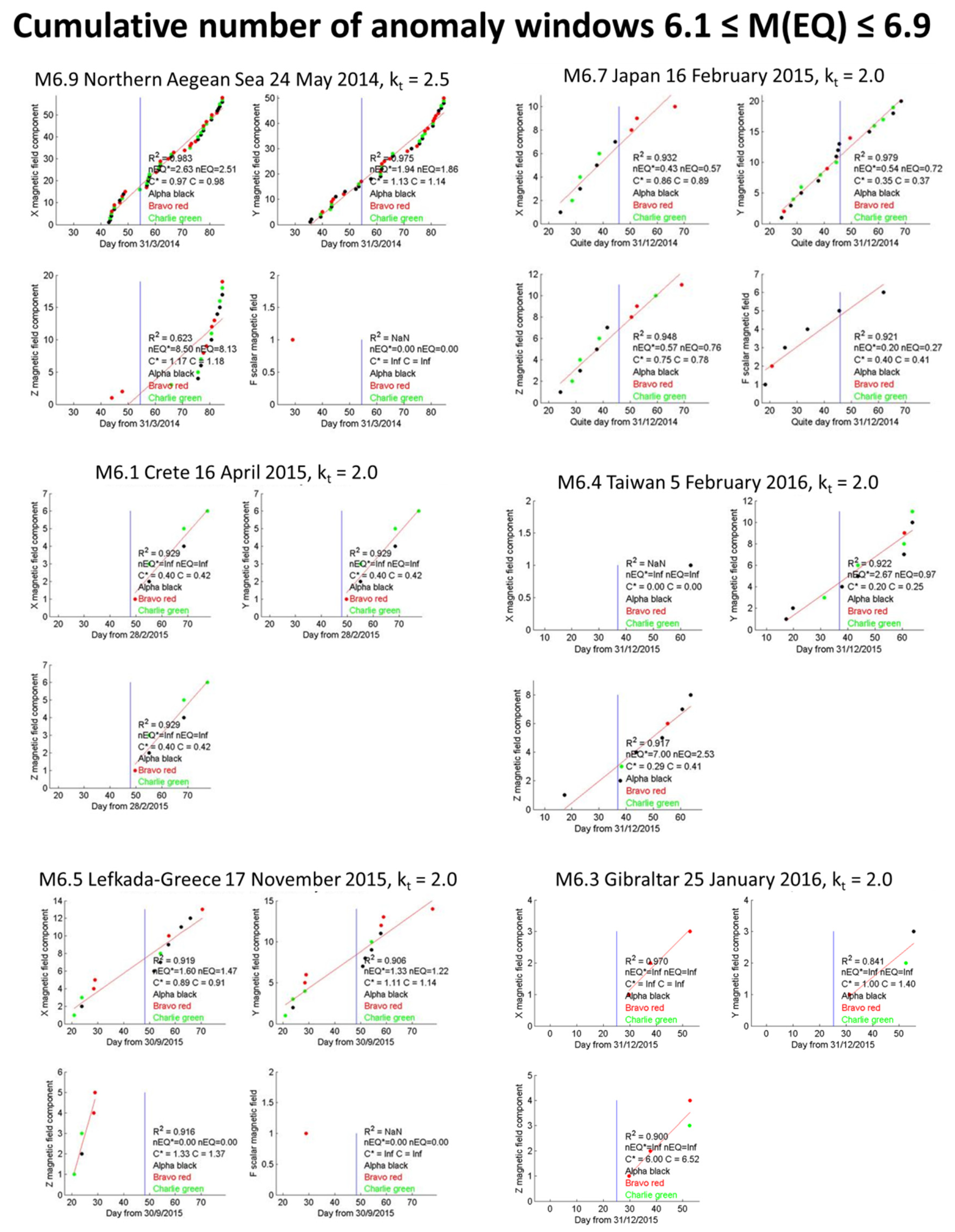
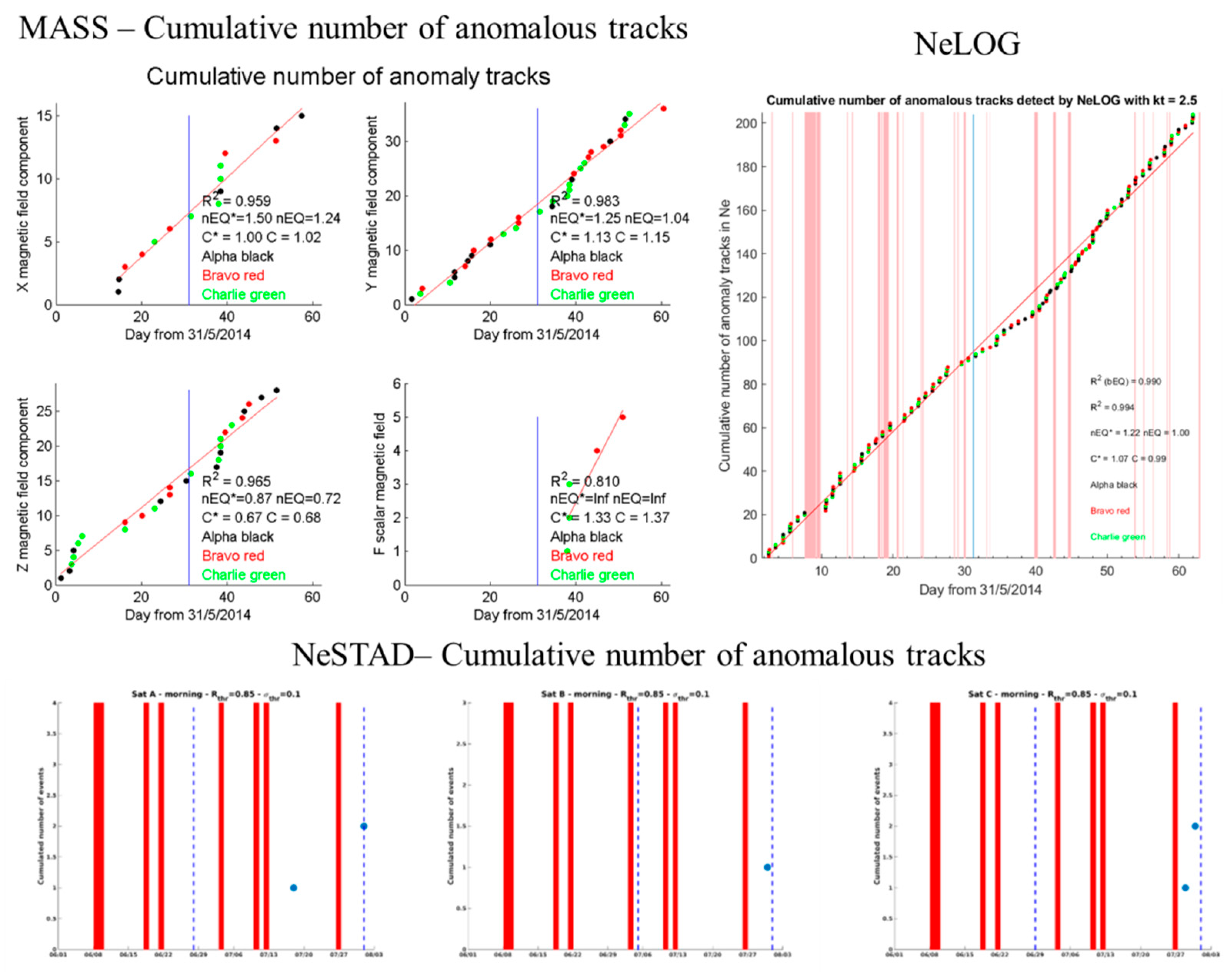
2.1. MASS Results
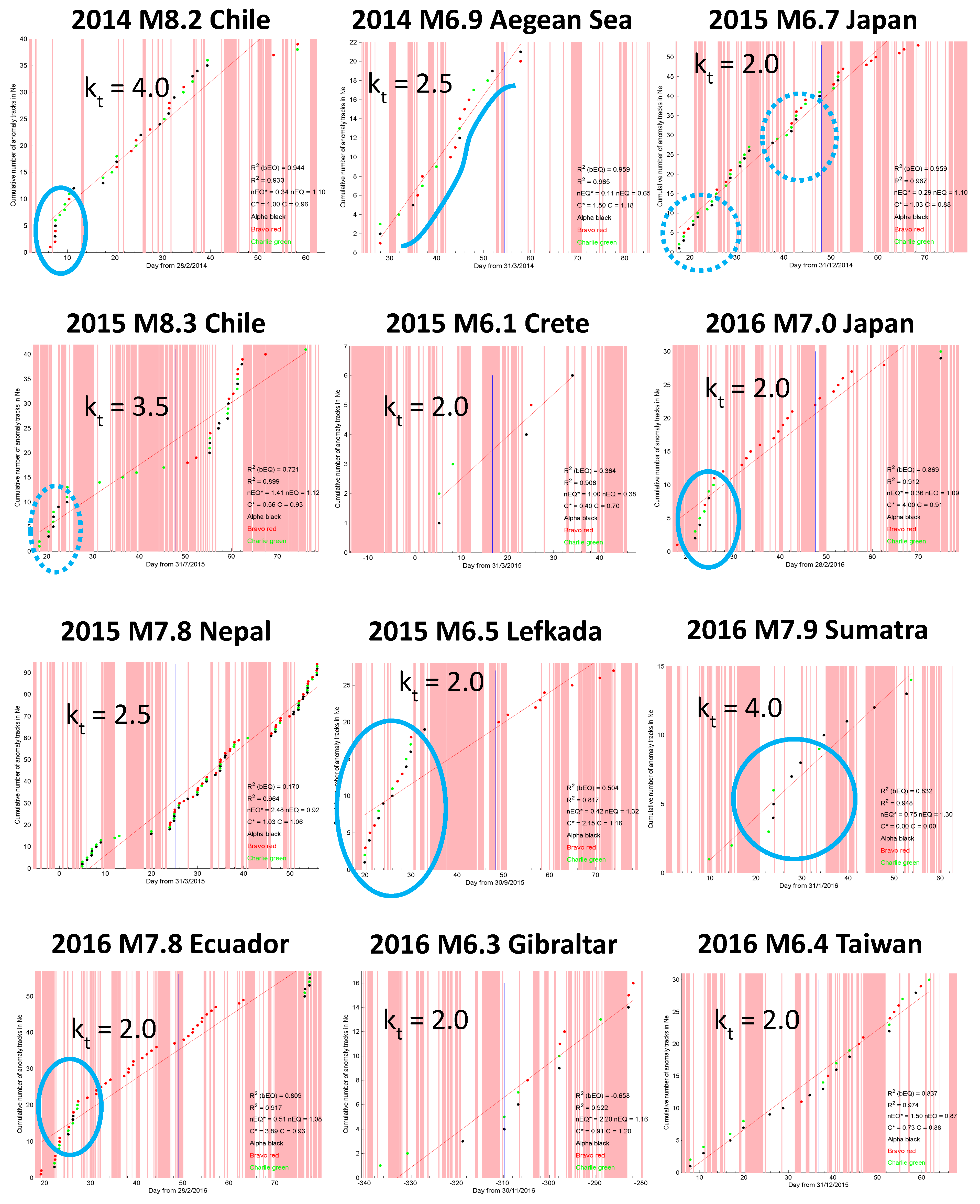
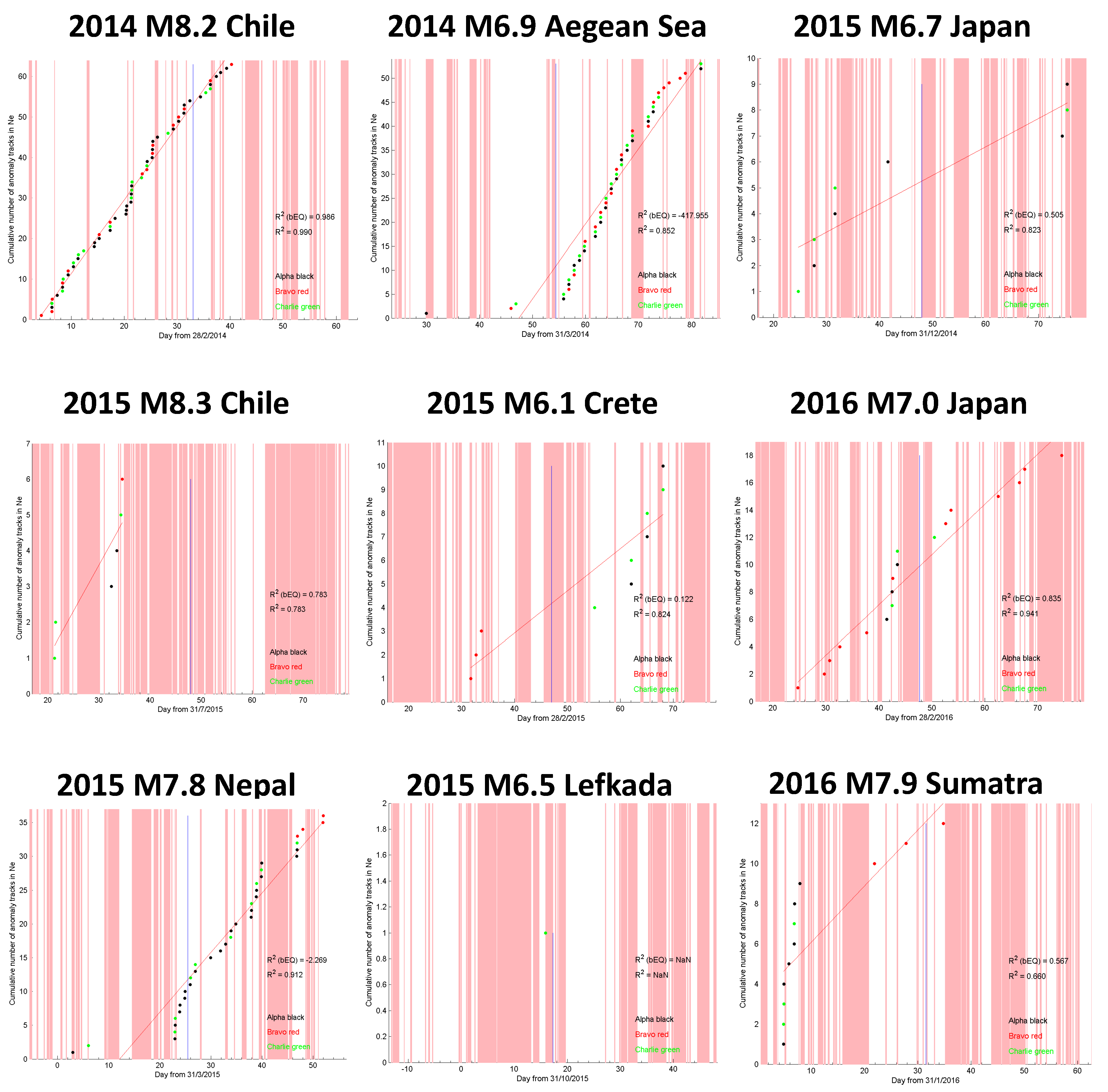
2.2. NeLOG Results
2.3. NeSTAD Results
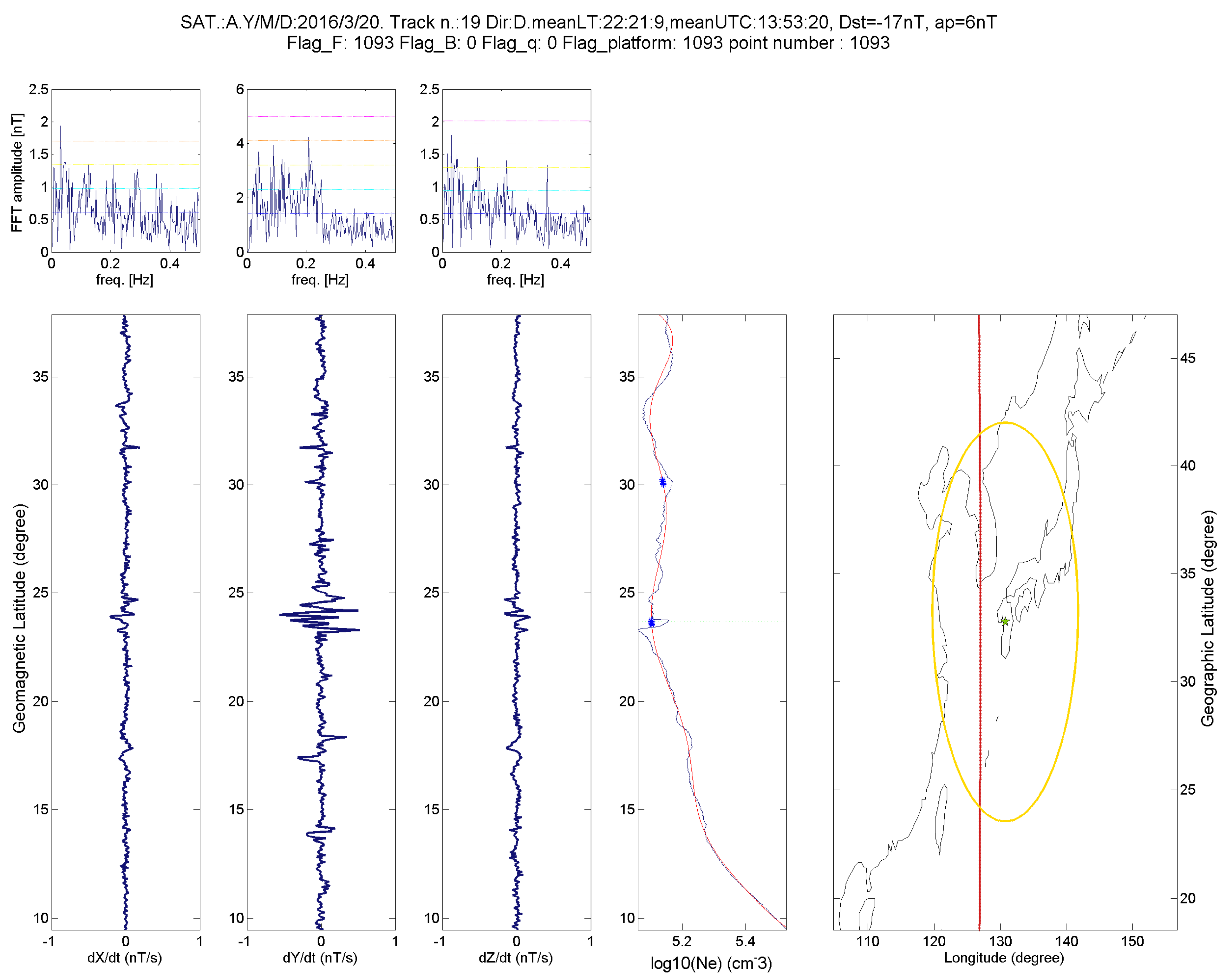
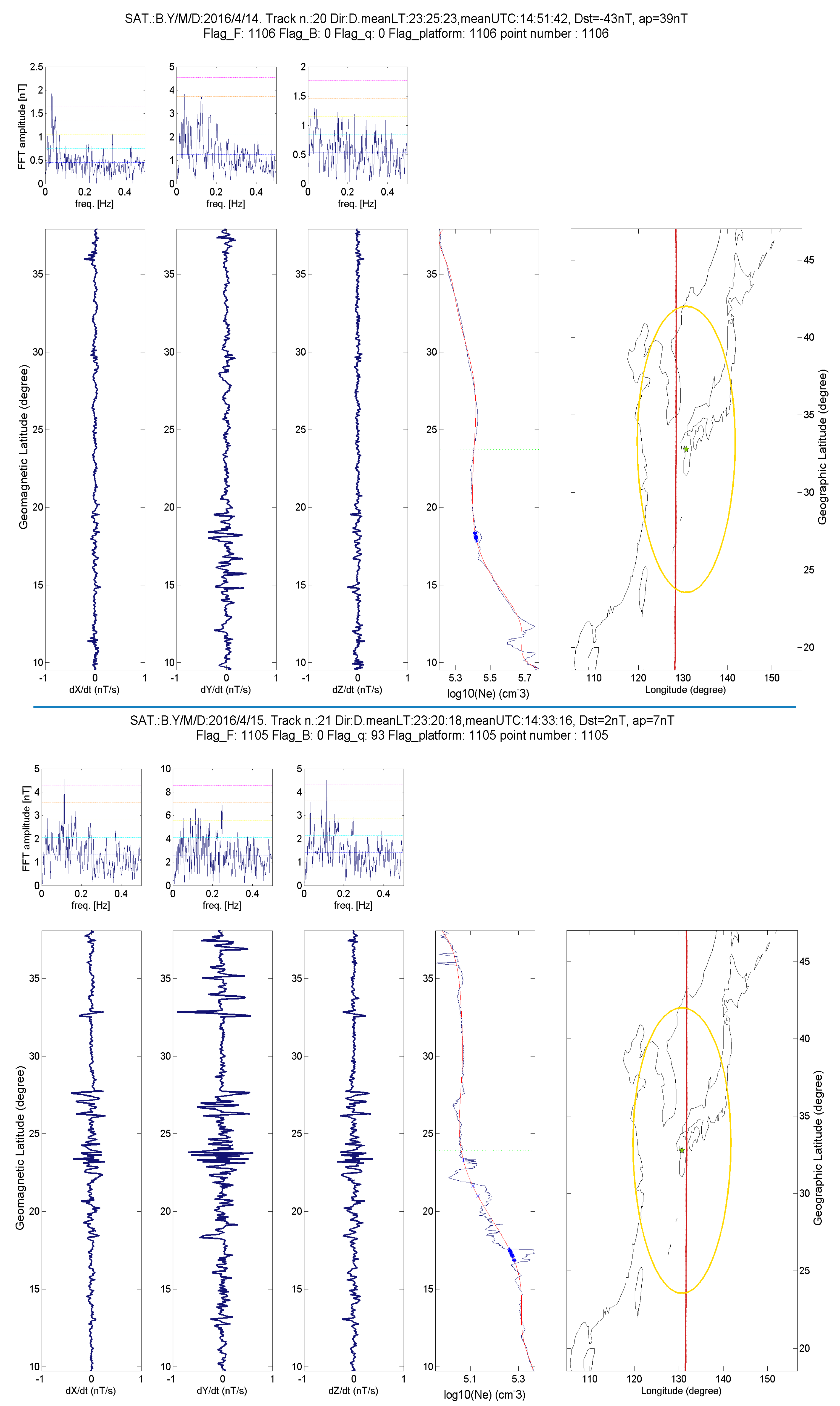
2.4. Example of Validation
2.5. Electron Density and Magnetic Field Concomitant Anomalies
2.6. Possible Lithospheric Origin of the Detected Anomalies
3. Discussion and Conclusions
4. Materials and Methods
4.1. Swarm Magnetic Field and Plasma Datasets
- a)
- Vector field magnetometer (VFM). It is a fluxgate magnetometer with a Compact Spherical Coil sensor, similar to the previous missions Oersted, CHAMP and SAC-C. The VFM data are provided at two time resolutions, High-Rate (HR, 50 Hz) and Low-Rate (LR, 1 Hz). The values of the geomagnetic field components are given in spherical coordinates (colatitude, latitude and radial distant) referred to the NEC (North, East, Center) frame and the time UTC. In this work we will use the Low-Rate (1 Hz) data.
- b)
- Absolute Scalar Magnetometer (ASM). It is based on the Electron Spin Resonance (ESR) principle using the Zeeman effect. The main objective of ASM is to calibrate the vector data. The instrument is located at the end of the boom, around 2 m distant from the VFM instrument. The ASM data are provided at 1 Hz rate.
- c)
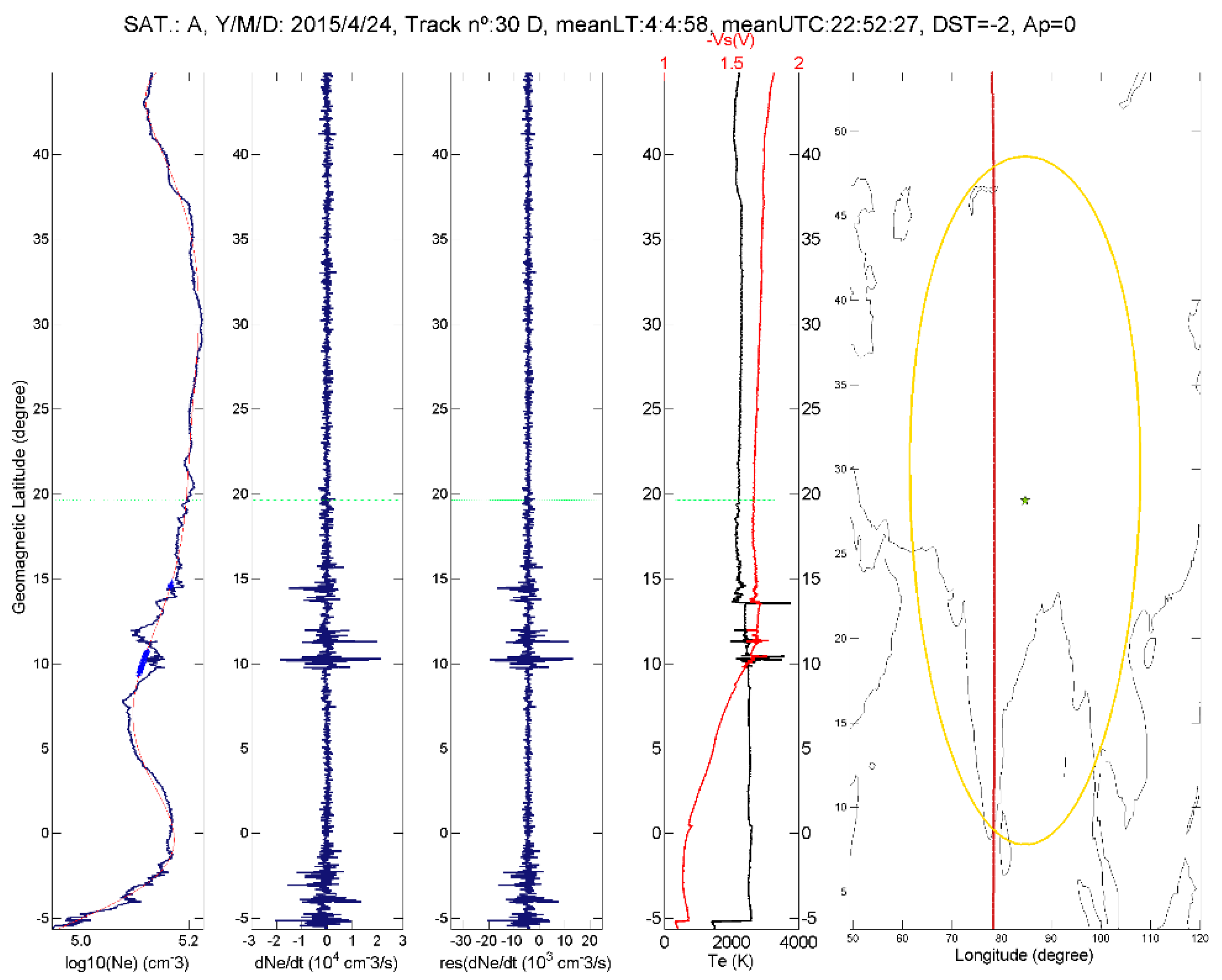
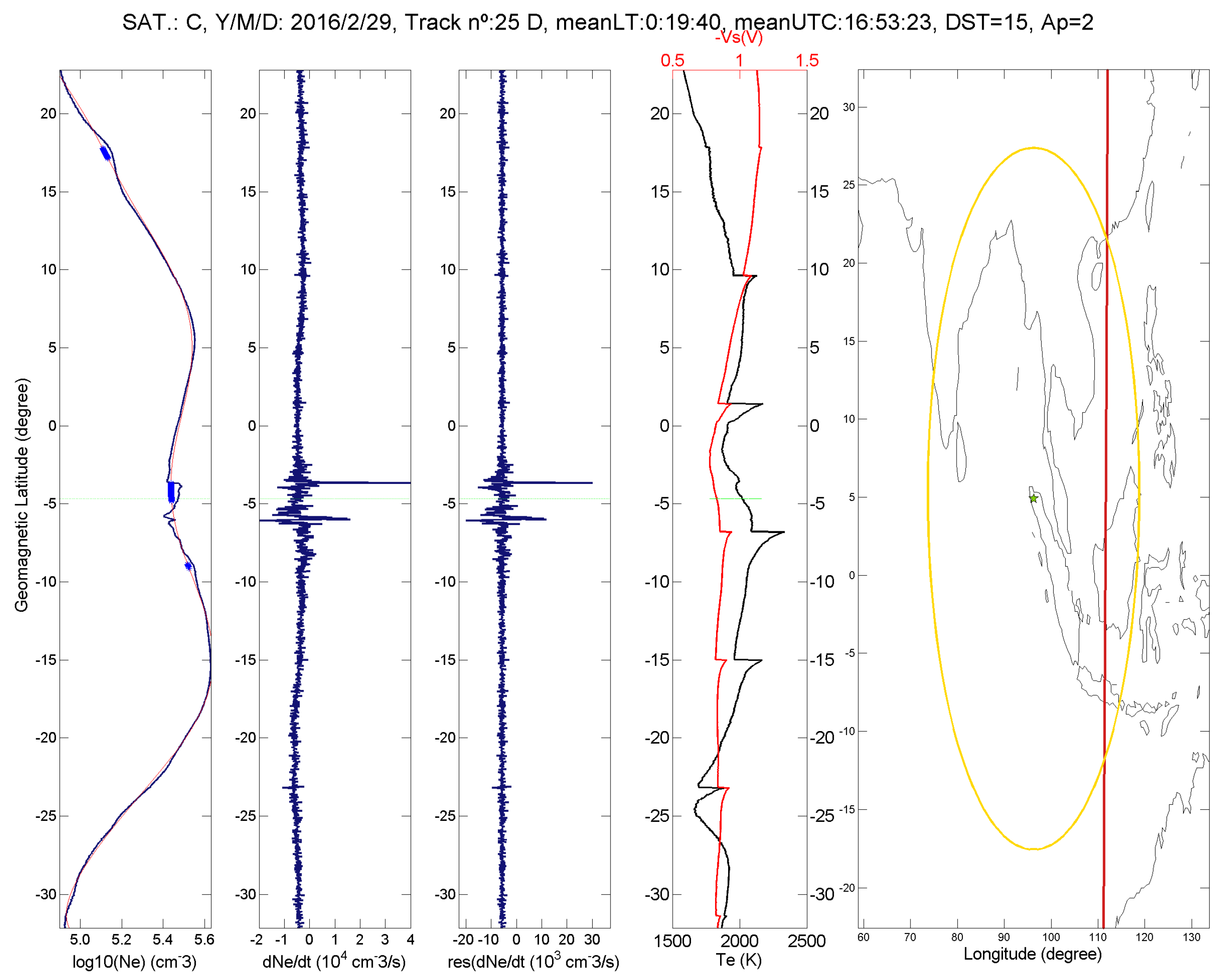
- Langmuir probe (LP). It determines the local properties of the plasma, such as temperature and density by measuring the collected current due to electrons and ions. In this paper, LP electron density, electron temperature and spacecraft potential data, stored in Swarm L1B EFIx_PL_1B product, are used. This kind of data is not the most updated, but for our purposes, they are adequate, because the variations are important, and not their absolute values. Data are provided at 2 Hz rate.
4.2. Earthquakes Selection: The 12 Case Studies
4.3. Description of the Algorithms
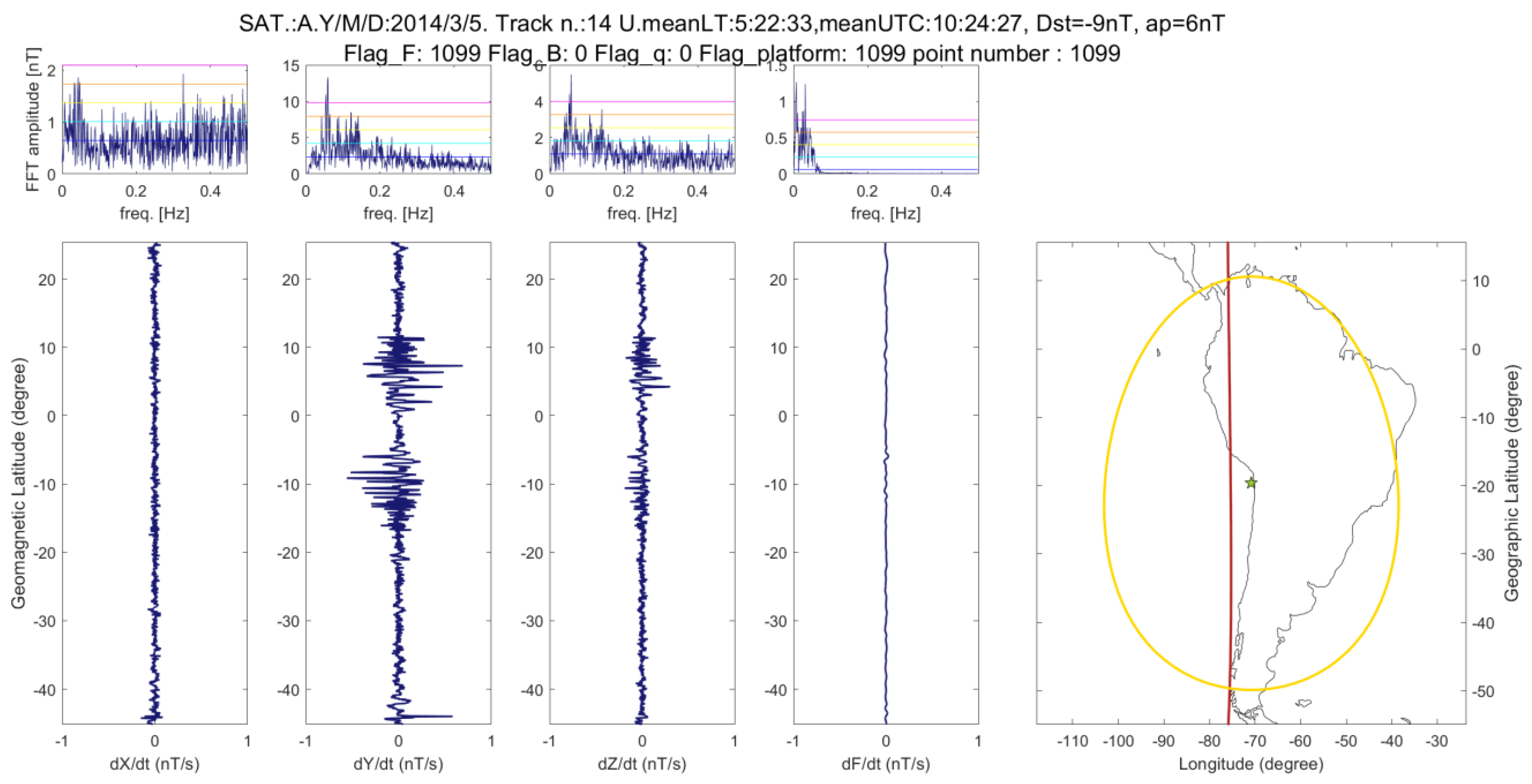
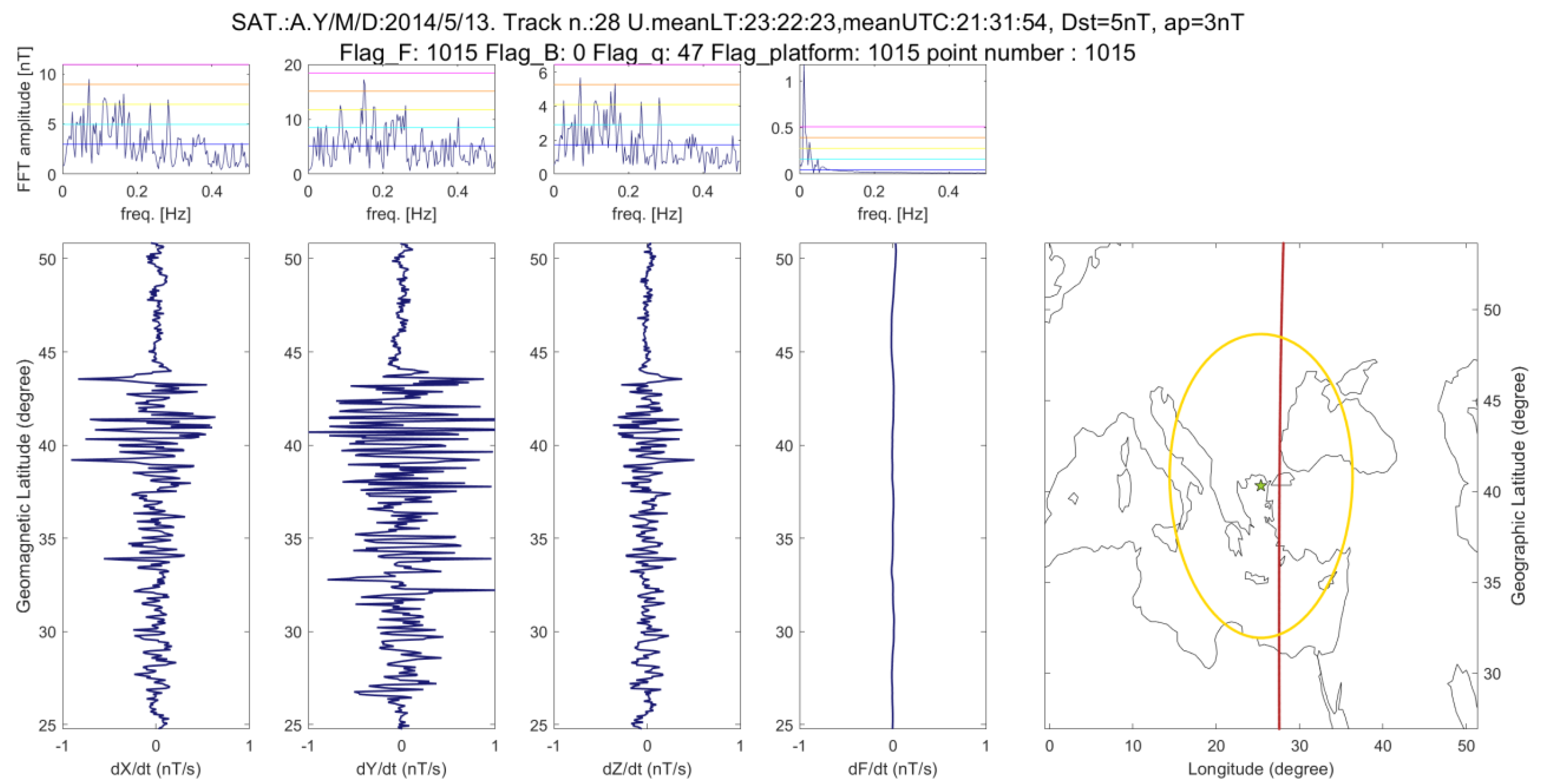
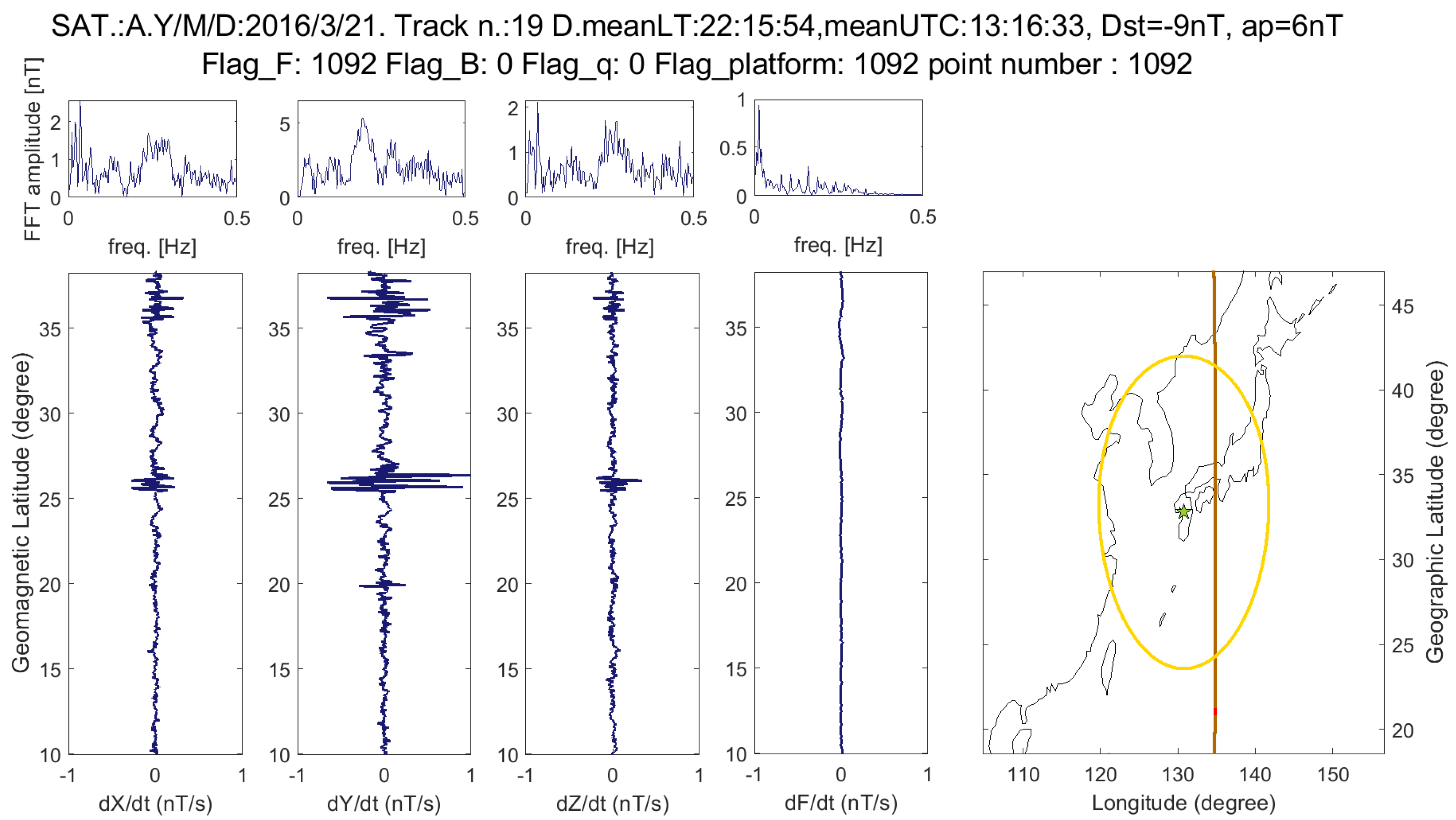
4.3.1. MASS Algorithm
- -
- To use a routine to analyse the satellite tracks and to separate them according to the local time. In a first attempt, the tracks with local time between 6 am and 10 pm were not used due to the influence of the external field, which increases in daytimes. After several night-time analyses, the study has been then extended to all daytime, too.
- -
- The first time derivative (in terms of first differences) is applied for each track in order to extract more information from the magnetic data, since in this way we remove part of the long trend and highlight the possible anomalies.
- -
- We remove the remaining long trend using a fitting by cubic splines. We choose the correct damping parameter and knot points for the splines in order to remove in a correct way the long spatial or temporal wavelengths of the magnetic data along the selected track.
- -
- Then, we apply the fitting to different geomagnetic field elements: the three orthogonal components X, Y, Z and the intensity F.
- -
- Finally and using the best fitting we analyse the residuals looking for a possible anomaly.
4.3.2. NeLOG Algorithm
4.3.3. NeSTAD Algorithm
- Swarm Langmuir Probe data: Swarm EFIx_PL (and Plasma Preliminary);
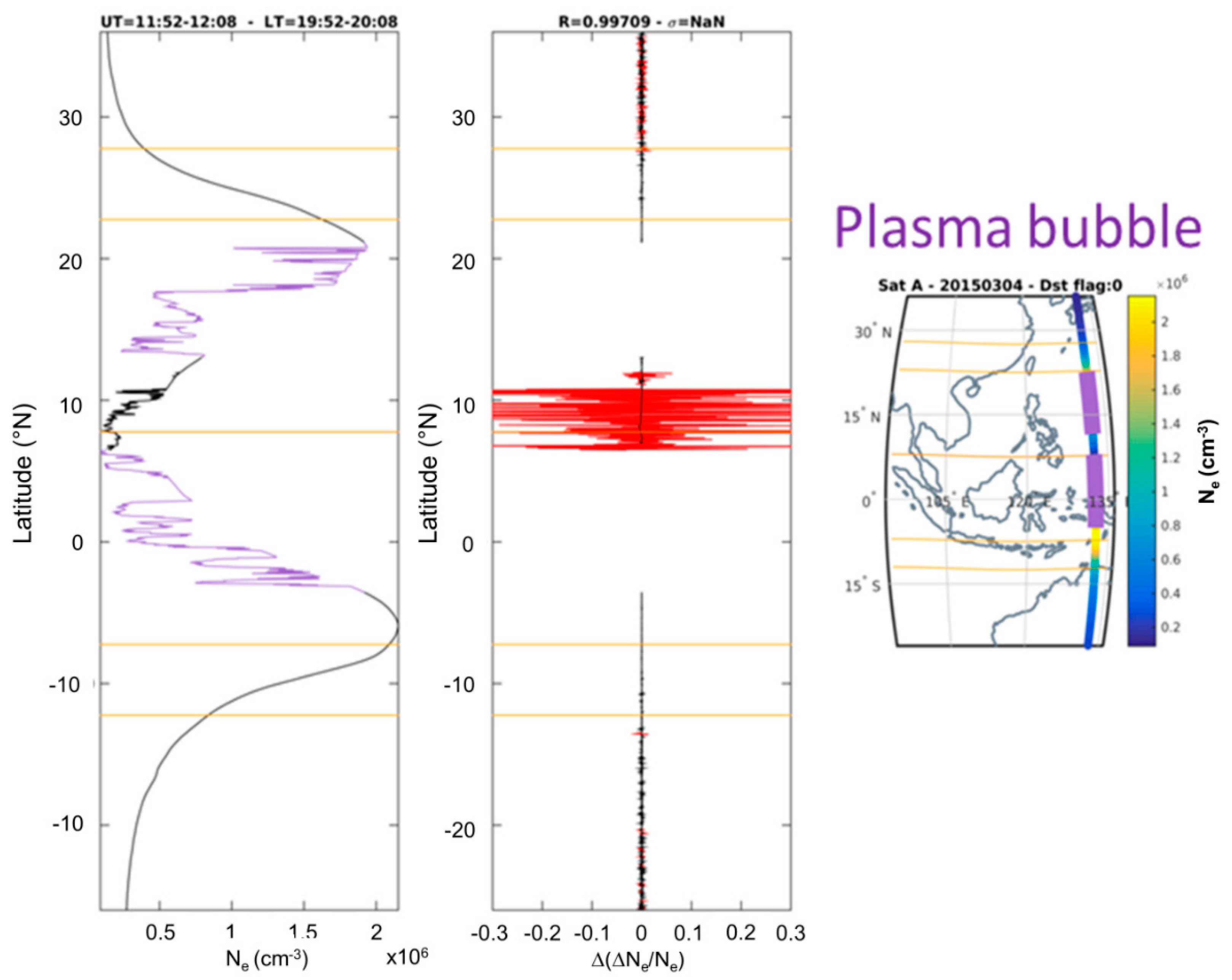
- Swarm Level 2 Ionospheric Bubble Index (IBI, Park et al. [55]);
- Dst index.
- 1)
- Manually selecting the boundaries in terms of minimum and maximum values of latitude and longitude
- 2)
- Selecting the center of the geographical range, i.e., the longitude-latitude coordinates (λ0, ϕ0), of the epicentre of a selected EQ, from which the geographical range is:
- Longitudinal extent = λ0 ± RDb (1 + ε);
- Latitudinal extent = Latitude = ϕ0 ± RDb (1 + ε);
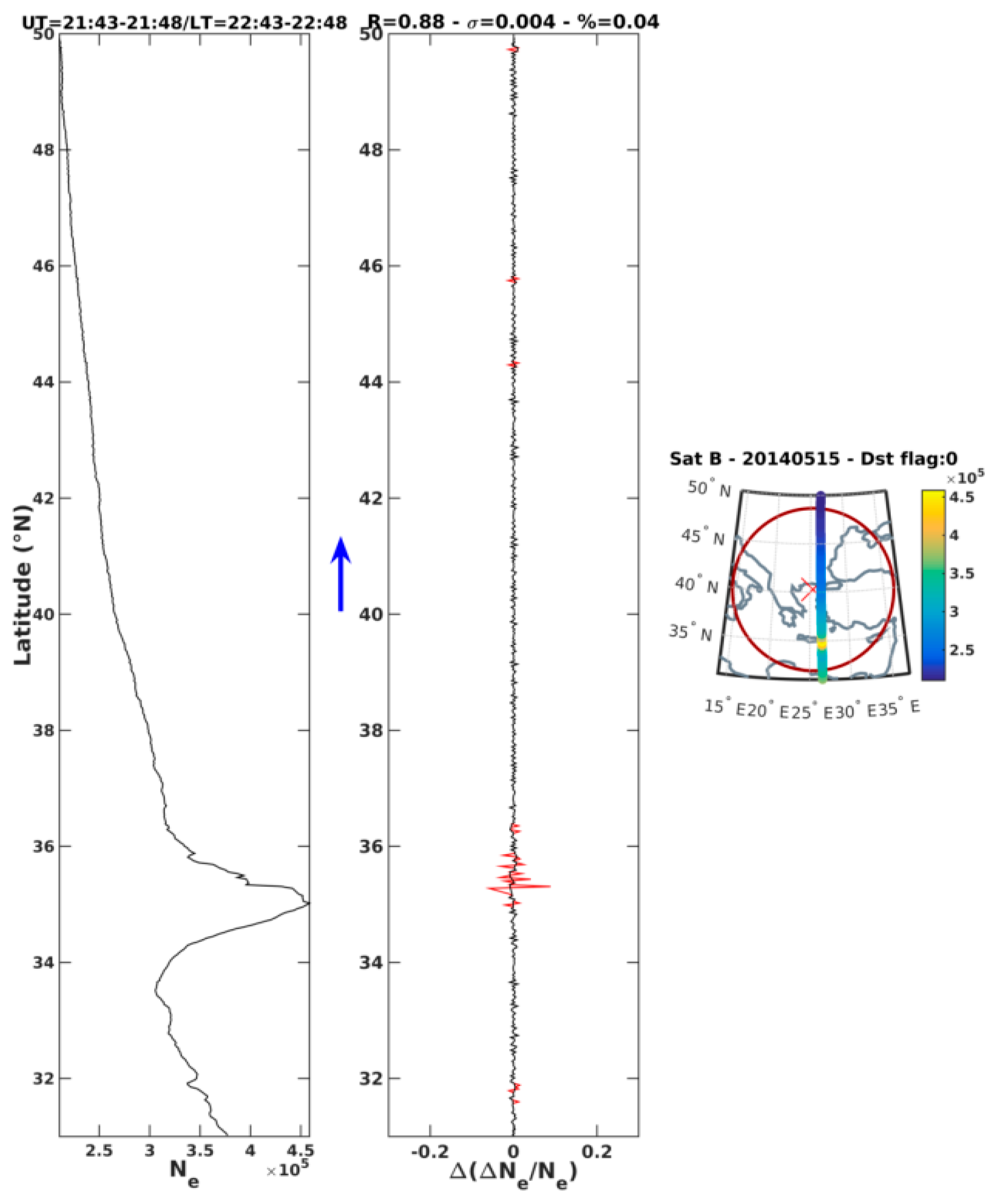
- : percentage difference between the maximum of the filtered () and of the original track ().
- σ: standard deviation of the distribution of the filtered track
- %: percentage of outliers identified in the track.
- Days before the event = 30
- Days after the event = 30
- Outliers k = 1.5 – mild outliers
- Case events at low latitudes
- R > Rthr = 0.85 i.e., only the strongly identified anomalies are taken into account, and standard deviation of the filtered track below σthr = 0.1 or standard deviation of the filtered track above σthr = 0.1 independently on R value.
- Morning tracks (02-06 LT), to remove the impact of the equatorial fountain during the day and to minimize the impact of the plasma bubble formation during night-time
- Case events at mid latitudes
- Rthr = 0.7 and standard deviation of the filtered track below σthr = 0.1 or standard deviation of the filtered track above σthr = 0.1 independently of the R value.
- Night time tracks (18 to 06 LT), because during night time and at mid latitudes the ionosphere is expected to be less turbulent.
- In both cases quiet ionospheric conditions (Dst flag = 0, i.e., absolute value of Dst in the considered day not exceeding 20 nT) are required.
Author Contributions
Funding
Acknowledgments
Conflicts of Interest
References
- Rawer, K. Wave Propagation in the Ionosphere; Springer: Dordrecht, The Netherlands, 1993. [Google Scholar]
- Kelley, M.C. The Earth’s Ionosphere: Plasma Physics and Electrodynamics (Vol. 96); Academic press: Cambridge, MA, USA, 2009. [Google Scholar]
- Hargreaves, J.K. The Solar-Terrestrial Environment: An Introduction to Geospace-the Science of the Terrestrial Upper Atmosphere, Ionosphere, and Magnetosphere; Cambridge University Press: Cambridge, UK, 1992. [Google Scholar]
- Laštovička, J. Forcing of the ionosphere by waves from below. J. Atmos. Sol-Terr. Phys. 2006, 3–5, 479–497. [Google Scholar] [CrossRef]
- Immel, T.J.; Mende, S.B.; Hagan, M.E.; Kintner, P.M.; England, S.L. Evidence of tropospheric effects on the ionosphere. Eos Trans. Am. Geophys. Union 2009, 9, 69–70. [Google Scholar] [CrossRef]
- Zettergren, M.D.; Snively, J.B. Ionospheric signatures of acoustic waves generated by transient tropospheric forcing. Geophys. Res. Lett. 2013, 20, 5345–5349. [Google Scholar] [CrossRef]
- Cesaroni, C.; Alfonsi, L.; Pezzopane, M.; Martinis, C.; Baumgardner, J.; Wroten, J.; Umbriaco, G. The first use of coordinated ionospheric radio and optical observations over Italy: Convergence of high-and low-latitude storm-induced effects. J. Geophys. Res. Space Phys. 2017, 11, 11,794–11,806. [Google Scholar] [CrossRef]
- Pulinets, S.A.; Boyarchuk, K.A. Ionospheric Precursors of Earthquakes; Springer Verlag: Berlin, Germany, 2004. [Google Scholar]
- Piša, D.; Nĕmec, F.; Santolik, O.; Parrot, M.; Rycroft, M. Additional attenuation of natural VLF electromagnetic waves observed by the DEMETER spacecraft resulting from preseismic activity. J. Geophys. Res. Space Phys. 2013, 118, 5286–5295. [Google Scholar] [CrossRef] [Green Version]
- De Santis, A.; Franceschi, De G.; Spogli, L.; Perrone, L.; Alfonsi, L.; Qamili, E.; Cianchini, G.; Di Giovambattista, R..; Salvi, S.; Filippi, E.; et al. Geospace perturbations induced by the Earth: The state of the art and future trends. Phys. Chem. Earth Parts A/B/C 2015, 85–86, 17–33. [Google Scholar] [CrossRef]
- Maruyama, T.; Tsugawa, T.; Kato, H.; Saito, A.; Otsuka, Y.; Nishioka, M. Ionospheric multiple stratifications and irregularities induced by the 2011 off the Pacific coast of Tohoku Earthquake. Earth Planets Space 2011, 7, 65. [Google Scholar] [CrossRef]
- Liu, J.Y.; Chen, C.H.; Lin, C.H.; Tsai, H.F.; Chen, C.H.; Kamogawa, M. Ionospheric disturbances triggered by the 11 March 2011 M9.0 Tohoku earthquake. J. Geophys Res. Space Phys. 2011, 116, A06319. [Google Scholar] [CrossRef]
- Freund, F.T. Pre-earthquake signals: Underlying physical processes. J. Asian Earth Sci. 2011, 41, 383–400. [Google Scholar] [CrossRef]
- Pulinets, S.A.; Ouzounov, O. Lithosphere–Atmosphere–Ionosphere Coupling (LAIC) model. An unified concept for earthquake precursors validation. J. Asian Earth Sci. 2011, 41, 371–382. [Google Scholar] [CrossRef]
- Breiner, S. Piezomagnetic effect at the time of local earthquakes. Nature 1964, 202, 790–791. [Google Scholar] [CrossRef]
- Moore, G.V. Magnetic disturbance preceding the 1964 Alaska earthquake. Nature 1964, 203, 508–509. [Google Scholar] [CrossRef]
- Stacey, F.D. Seismo-magnetic effect and the possibility of forecasting earthquakes. Nature 1963, 200, 1083. [Google Scholar] [CrossRef]
- Fraser-Smith, A.C.; Bernardi, A.; McGill, P.R.; Ladd, M.E.; Helliwell, R.A.; Villard, O.G. Low-frequency magnetic field measurements near the epicenter of the Ms 7.1 Loma Prieta earthquake. Geophys. Res. Lett. 1990, 17, 1465–1468. [Google Scholar] [CrossRef]
- Molchanov, O.A.; Kopytenko, Yu.A.; Voronov, P.M.; Kopytenko, E.A.; Matiashvili, T.G.; Fraser-Smith, A.C.; Bernardi, A. Results of ULF magnetic field measurements near the epicenters of the Spitak (Ms = 6.9) and Loma Prieta (Ms = 7.1) earthquakes: Comparative analysis. Geophys. Res. Lett. 1992, 19, 1495–1498. [Google Scholar] [CrossRef]
- Donner, R.V.; Potirakis, S.M.; Balasis, G.; Eftaxias, K.; Kurths, J. Temporal correlation patterns in pre-seismic electromagnetic emissions reveal distinct complexity profiles prior to major earthquakes. Phys. Chem. Earth Parts A/B/C 2015, 86, 44–55. [Google Scholar] [CrossRef]
- Gaffet, S.; Guglielmi, Y.; Virieux, J.; Waysand, G.; Chwala, A.; Stolz, R.; Emblanch, C.; Auguste, M.; Boyer, D.; Cavaillou, A. Simultaneous seismic and magnetic measurements in the Low-Noise Underground Laboratory (LSBB) of Rustrel, France, during the 2001 January 26 Indian earthquake. Geophys. J. Int. 2003, 155, 981–990. [Google Scholar] [CrossRef]
- Larkina, V.I.; Nalivayko, A.V.; Gershenzon, N.I.; Gokhberg, M.; Liperovskiy, V.A.; Shalimov, S.L. Observation of VLF emission, related with seismic activity, on the Interkosmos-19 satellite. Geomagn. Aeron. 1984, 23, 684–687. [Google Scholar]
- Hayakawa, M.; Kawate, R.; Molchanov, O.A.; Yumoto, K. Results of ultra-low frequency magnetic field measurements during the Guam earthquake of 8 August 1993. Geophys. Res. Lett. 1996, 3, 241–244. [Google Scholar] [CrossRef]
- Galperin, Yu. I.; Hayakawa, M. On the Magnetospheric Effects of Experimental Ground Explosions Observed from AUREOL-3. J. Geomagn. Geoelectr. 1996, 48, 1241. [Google Scholar] [CrossRef]
- Parrot, M. Use of satellites to detect seismo-electromagnetic effects. Adv. Space Res. 1995, 15, 27–35. [Google Scholar] [CrossRef]
- Johnston, M.J.S. Review of electric and magnetic fields accompanying seismic and volcanic activity. Surv. Geophys. 1997, 18, 441–475. [Google Scholar] [CrossRef]
- Zlotnicki, J.; Nisida, Y. Review of morphological insights of self-potential anomalies on volcano. Surv. Geophys. 2003, 24, 291–338. [Google Scholar] [CrossRef]
- Eftaxias, K.; Contoyiannis, Y.; Balasis, G.; Karamanos, K.; Kopanas, J.; Antonopoulos, G.; Koulouras, G.; Nomicos, C. Evidence of fractional-Brownian-motion-type asperity model for earthquake generation in candidate pre-seismic electromagnetic emissions. Nat. Hazards Earth Syst. Sci. 2008, 8, 657–669. [Google Scholar] [CrossRef] [Green Version]
- Finkelstein, M.; Price, C.; Eppelbaum, L. Is the geodynamic process in preparation of strong earthquakes reflected in the geomagnetic field? J. Geophys. Eng. 2012, 9, 585–594. [Google Scholar] [CrossRef]
- Balasis, G.; Daglis, I.A.; Georgiou, M.; Papadimitriou, C.; Haagmans, R. Magnetospheric ULF wave studies in the frame of Swarm mission: A time-frequency analysis tool for automated detection of pulsations in magnetic and electric field observations. Earth Planet. Space 2013, 11, 18. [Google Scholar] [CrossRef]
- Balasis, G.; Papadimitriou, C.; Boutsi, A.Z. Ionospheric response to solar and interplanetary disturbances: A Swarm perspective. Philos. Trans. R. Soc. A 2019, 2148. [Google Scholar] [CrossRef]
- Balasis, G.; Mandea, M. Can electromagnetic disturbances related to the recent great earthquakes be detected by satellite magnetometers? Tectonophysics 2007, 431, 173–195. [Google Scholar] [CrossRef]
- Mandea, M.; Balasis, G. The SGR 1806-20 magnetar signature on the Earth’s magnetic field. Geophys. J. Int. 2006, 2, 586–591. [Google Scholar] [CrossRef]
- Ryu, K.; Chae, J.S.; Lee, E.; Parrot, M. Fluctuations in the ionosphere related to Honshu Twin Large Earthquakes of September 2004 observed by the DEMETER and CHAMP satellites. J. Atmos. Sol-Terr. Phys. 2014, 121, 110–122. [Google Scholar] [CrossRef]
- Ryu, K.; Parrot, M.; Kim, S.G.; Jeong, K.S.; Chae, J.S.; Pulinets, S.; Oyama, K.I. Suspected seismo-ionospheric coupling observed by satellite measurements and GPS TEC related to the M7.9 Wenchuan earthquake of 12 May 2008. J. Geophys. Res. Space Phys. 2014, 12, 10–305. [Google Scholar] [CrossRef]
- Ryu, K.; Oyama, K.I.; Bankov, L.; Chen, C.H.; Devi, M.; Liu, H.; Liu, J.Y. Precursory enhancement of EIA in the morning sector: Contribution from mid-latitude large earthquakes in the north-east Asian region. Adv. Space Res. 2016, 57, 268–280. [Google Scholar] [CrossRef]
- Wang, Y.D.; Pi, D.C.; Zhang, X.M.; Shen, X.H. Seismo-ionospheric precursory anomalies detection from DEMETER satellite data based on data mining. Nat. Hazards 2015, 76, 823–837. [Google Scholar] [CrossRef]
- Akhoondzadeh, M. Ant Colony Optimization detects anomalous aerosol variations associated with the Chile earthquake of 27 February 2010. Adv. Space Res. 2015, 55, 1754–1763. [Google Scholar] [CrossRef]
- Hazra, P.; Islam, T. Proton Density Variation in Ionosphere Before Strong Earthquake Using GOES-15 Data. In Computational Advancement in Communication Circuits and Systems; Maharatna, K., Dalapati, G., Banerjee, P., Mallick, A., Mukherjee, M., Eds.; Lecture Notes in Electrical Engineering, Vol 335; Springer: New Delhi, India, 2015. [Google Scholar]
- Akhoondzadeh, M.; De Santis, A.; Marchetti, D.; Piscini, A.; Cianchini, G. Multi precursors analysis associated with the powerful Ecuador (MW=7.8) earthquake of 16 April 2016 using Swarm satellites data in conjunction with other multi-platform satellite and ground data. Adv. Space Res. 2018, 61, 248–263. [Google Scholar] [CrossRef]
- De Santis, A.; Balasis, G.; Pavón-Carrasco, F.J.; Cianchini, G.; Mandea, M. Potential earthquake precursory pattern from space: The 2015 Nepal event as seen by magnetic Swarm satellites. Earth Planet. Sci. Lett. 2017, 461, 119–126. [Google Scholar] [CrossRef] [Green Version]
- Marchetti, D.; Akhoondzadeh, M. Analysis of Swarm satellites data showing seismo-ionospheric anomalies around the time of the strong Mexico (Mw=8.2) earthquake of 08 September 2017. Adv. Space Res. 2018, 62, 614–623. [Google Scholar] [CrossRef]
- Akhoondzadeh, M.; De Santis, A.; Marchetti, D.; Piscini, A.; Jin, S. Anomalous seismo-LAI variations potentially associated with the 2017 Mw=7.3 Sarpol-e Zahab (Iran) earthquake from Swarm satellites, GPS TEC and climatological data. Adv. Space Res. 2019, 64, 143–158. [Google Scholar] [CrossRef]
- Marchetti, D.; De Santis, A.; D’Arcangelo, S.; Poggio, F.; Jin, S.; Piscini, A.; Campuzano, S.A. Magnetic Field and Electron Density Anomalies from Swarm Satellites Preceding the Major Earthquakes of the 2016–2017 Amatrice-Norcia (Central Italy) Seismic Sequence. Pure Appl. Geophs. 2019, in press. [Google Scholar] [CrossRef]
- Lay, T.; Yue, H.; Brodsky, E.E.; An, C. The 1 April 2014 Iquique, Chile, Mw8.1 earthquake rupture sequence. Geophys. Res. Lett. 2014, 41, 3818–3825. [Google Scholar] [CrossRef]
- Dobrovolsky, I.P.; Zubkov, S.I.; Miachkin, V.I. Estimation of the size of earthquake preparation zones. PAGEOPH 1979, 117, 1025. [Google Scholar] [CrossRef]
- Friis-Christensen, E.; Lühr, H.; Hulot, G. Swarm: A constellation to study the Earth’s magnetic field. Earth Planets Space 2006, 58, 351–358. [Google Scholar] [CrossRef]
- “Swarm-L1b-Product-Definition”. Available online: https://earth.esa.int/web/guest/missions/esa-eo-missions/swarm/data-handbook/level-1b-product-definitions (accessed on 17 January 2019).
- United States Geological Survey. Available online: https://earthquake.usgs.gov/earthquakes/search/ (accessed on 11 February 2019).
- Perrone, L.; De Franceschi, G. Solar, ionospheric and geomagnetic indices. Ann. Geophys. 1998, 5–6, 843–855. [Google Scholar]
- Word Data Centre for Geomagnetism, Kyoto University. Available online: http://wdc.kugi.kyoto-u.ac.jp/wdc/Sec3.html (accessed on 11 February 2019).
- SAFE Project web site. Available online: http://safe-swarm.ingv.it/resources/data/earthquakes-boards. (accessed on 25 May 2019).
- Plastino, W.; Bella, F.; Catalano, P.G.; Di Giovambattista, R. Radon groundwater anomalies related to the Umbria–Marche, September 26, 1997. Earthq. Geofis. Int. 2002, 4, 369–375. [Google Scholar]
- Vizzini, F.; Brai, M. In-soil radon anomalies as precursors of earthquakes: A case study in the SE slope of Mt. Etna in a period of quite stable weather conditions. J. Environ. Radioact. 2012, 113, 131–141. [Google Scholar] [CrossRef]
- Park, J.; Noja, M.; Stolle, C.; Lühr, H. The Ionospheric Bubble Index deduced from magnetic field and plasma observations onboard Swarm. Earth Planets Space 2013, 11, 13. [Google Scholar] [CrossRef]
- Balan, N.; Liu, L.; Le, H. A brief review of equatorial ionization anomaly and ionospheric irregularities. Earth Planet. Phys. 2018, 4, 257–275. [Google Scholar] [CrossRef]
- Spogli, L.; Cesaroni, C.; Di Mauro, D.; Pezzopane, M.; Alfonsi, L.; Musicò, E.; Linty, N. Formation of ionospheric irregularities over Southeast Asia during the 2015 St. Patrick’s Day storm. J. Geophys. Res. Space Phys. 2016, 12, 12,211–12,233. [Google Scholar] [CrossRef]
- Balasis, G.; Papadimitriou, C.; Daglis, I.A.; Pilipenko, V. ULF wave power features in the topside ionosphere revealed by Swarm observations. Geophys. Res. Lett. 2015, 17, 6922–6930. [Google Scholar] [CrossRef]
- Barnett, V.; Lewis, T. Outliers in Statistical Data, 3rd ed.; J. Wiley & Sons: Hoboken, NJ, USA, 1994; XVII; 582p. [Google Scholar]
- Cander, L.R.; Mihajlovic, S.J. Ionospheric spatial and temporal variations during the 29–31 October 2003 storm. J. Atmos. Sol-Terr. Phys. 2005, 67, 1118–1128. [Google Scholar] [CrossRef]


| # | Earthquake | MASS | NeSTAD | NeLOG |
|---|---|---|---|---|
| 1 | Chile 2014 M8.2 | ~ | ~ | Ok! |
| 2 | N. Aegean Sea 2014 M6.9 | ~ | No | ~ |
| 3 | Nepal 2015 M7.8 | Ok! | Ok! | Ok! |
| 4 | Chile 2015 M8.3 | Ok! | ~ | Ok! |
| 5 | Japan 2015 M6.7 | Ok! | ~ | ~ |
| 6 | Japan 2016 M7.0 | Ok! | Ok! | Ok! |
| 7 | Ecuador 2016 M7.8 | Ok! | No | ~ |
| 8 | Sumatra 2016 M7.9 | Ok! | ~ | Ok! |
| 9 | Crete 2015 M6.1 | No | ~ | No |
| 10 | Lefkada 2015 M6.5 | ~ | No | ~ |
| 11 | Gibraltar 2016 M6.3 | No | No | Ok! |
| 12 | Taiwan 2016 M6.4 | Ok! | No | Ok! |
| Location | Latitude Epicenter | Longitude Epicenter | Date and Time (UTC) | Magnitude | Depth (km) |
|---|---|---|---|---|---|
| Chile (Illapel) | 31.573° S | 71.674° W | 16/09/2015 22:54:32 | 8.3 | 22.4 |
| Chile-Iquique (Land) | 19.642° S | 70.817° W | 01/04/2014 23:46:46 | 8.2 | 20.1 |
| Offshore Sumatra | 4.952° S | 94.330° E | 02/03/2016 12:49:48 | 7.9 | 24.0 |
| Nepal (Gorkha) | 28.230° N | 84.731° E | 25/04/2015 6:11:25 | 7.8 | 8.2 |
| Ecuador (Muisne) | 0.382° N | 79.922° W | 16/04/2016 23:58:36 | 7.8 | 20.6 |
| Japan (Kumamoto-shi) | 32.791° N | 130.754° E | 15/4/2016 16:25:06 | 7.0 | 10.0 |
| Northern Aegean Sea | 40.289° N | 25.389° E | 24/05/2014 9:25:02 | 6.9 | 6.4 |
| Japan (Miyako) | 39.856° N | 142.881° E | 16/02/2015 23:06:28 | 6.7 | 23.0 |
| Greece (Lefkada-Nidri) | 38.670° N | 20.600° E | 17/11/2015 7:10:07 | 6.5 | 11.0 |
| Taiwan | 22.938° N | 120.601° E | 05/02/2016 19:57:27 | 6.4 | 23.0 |
| Strait of Gibraltar | 35.649° N | 3.682° W | 25/01/2016 4:22:02 | 6.3 | 12.0 |
| Greece (Kasos-Crete) | 35.189° N | 26.823° E | 16/04/2015 18:07:43 | 6.1 | 20.0 |
| Dst Flag | Dst Conditions | Geomagnetic Conditions |
|---|---|---|
| −1 | Dst data not available | Dst data not available |
| 0 | −20 ≤ Dstmin ≤ 20 nT | Quiet day |
| 1 | −100 < Dstmin < −20 nT | Disturbed period |
| 2 | −250 < Dstmin < −100 nT | Severe storm |
| 3 | Dstmin < −250 nT | Extreme event |
© 2019 by the authors. Licensee MDPI, Basel, Switzerland. This article is an open access article distributed under the terms and conditions of the Creative Commons Attribution (CC BY) license (http://creativecommons.org/licenses/by/4.0/).
Share and Cite
De Santis, A.; Marchetti, D.; Spogli, L.; Cianchini, G.; Pavón-Carrasco, F.J.; Franceschi, G.D.; Di Giovambattista, R.; Perrone, L.; Qamili, E.; Cesaroni, C.; et al. Magnetic Field and Electron Density Data Analysis from Swarm Satellites Searching for Ionospheric Effects by Great Earthquakes: 12 Case Studies from 2014 to 2016. Atmosphere 2019, 10, 371. https://doi.org/10.3390/atmos10070371
De Santis A, Marchetti D, Spogli L, Cianchini G, Pavón-Carrasco FJ, Franceschi GD, Di Giovambattista R, Perrone L, Qamili E, Cesaroni C, et al. Magnetic Field and Electron Density Data Analysis from Swarm Satellites Searching for Ionospheric Effects by Great Earthquakes: 12 Case Studies from 2014 to 2016. Atmosphere. 2019; 10(7):371. https://doi.org/10.3390/atmos10070371
Chicago/Turabian StyleDe Santis, Angelo, Dedalo Marchetti, Luca Spogli, Gianfranco Cianchini, F. Javier Pavón-Carrasco, Giorgiana De Franceschi, Rita Di Giovambattista, Loredana Perrone, Enkelejda Qamili, Claudio Cesaroni, and et al. 2019. "Magnetic Field and Electron Density Data Analysis from Swarm Satellites Searching for Ionospheric Effects by Great Earthquakes: 12 Case Studies from 2014 to 2016" Atmosphere 10, no. 7: 371. https://doi.org/10.3390/atmos10070371