Nutrient-Dense Crops for Rural and Peri-Urban Smallholders in Kenya—A Regional Social Accounting Approach


1
Institute for Environmental Economics and World Trade, Leibniz Universität Hannover, Königsworther Platz 1, 30167 Hannover, Germany
2
Environmental and Development Economics, TUM Campus Straubing for Biotechnology and Sustainability, Technical University of Munich, HSWT, Petersgasse 18, 94315 Straubing, Germany
*
Author to whom correspondence should be addressed.
Sustainability 2019, 11(11), 3017; https://doi.org/10.3390/su11113017
Submission received: 26 April 2019
/
Revised: 20 May 2019
/
Accepted: 24 May 2019
/
Published: 28 May 2019
(This article belongs to the Special Issue Agricultural Development and Food Security in Developing Countries: Innovations and Sustainability)
Abstract
:Kenya ranks among the countries with the highest micronutrient deficiency worldwide. Due to their high micronutrient content, African indigenous vegetables (AIVs) can be a solution to this problem, and urban areas in Kenya have seen a rise in demand for these crops in the previous decade. To fill the gap between supply and demand, programmes to promote AIV production have been implemented in rural and peri-urban areas. However, the effects of increased AIV production on income and food security in the regional economies are not clear. Thus, in this analysis, we first evaluate differences between the livelihoods of household groups with different levels of food security in rural and peri-urban Kenya using a two-step cluster analysis. Then, we generate a regional social accounting matrix (SAM) and calculate the direct and indirect income effects of AIVs and other crops grown in the area using a multiplier analysis. For the analysis, a total of 706 small-scale vegetable producers in four counties in Kenya were interviewed in 2015. Households in rural areas were more food insecure, especially with respect to the utilization and stability dimension of food security. Multiplier analysis showed increased indirect income effects of AIVs in the regional economy compared to those of many cash crops. We suggest further promoting the production of AIVs in rural and peri-urban Kenya.
1. Introduction
With approximately 20% of its population undernourished, Kenya still ranks among the top countries with micronutrient deficiencies worldwide [1,2]. Unfavourable rains and an unstable agricultural system have worsened the situation in recent years [3]. African indigenous vegetables (AIVs) have very high levels of micronutrients and are thus a suitable tool to combat food insecurity, especially micronutrient deficiencies [4,5]. Because of their increasing popularity, AIVs have seen a rise in their appreciation and demand in urban areas in Kenya in the previous decade, leading to the increased production of these crops [6].
The agricultural sector often plays a very important role in not only the livelihoods of the farmers themselves but also the economic development of the entire region in which they are based because the agricultural sector is connected to other sectors such as food processing facilities, traders and input suppliers [7]. Thus, an increase in AIV demand in urban markets can increase the welfare of many households in Kenya’s rural and peri-urban regions not only directly through an increase in AIV production but also indirectly through the creation of employment opportunities and hence higher purchasing power for other commodities [8]. In light of increasing urbanization in Kenya, strengthening these economic linkages between rural areas and urban markets can foster the economic development of the entire country [8,9].
Despite the potential of AIVs to increase food security and generate income, their role in the Kenyan economy has rarely been analysed. Whether farmers benefit from adopting AIVs as cash crops depends on the local context [10,11,12], and an analysis of the regional differences between rural and peri-urban Kenya is urged. This paper aims to fill this gap with a regional social accounting matrix (SAM) that evaluates who benefits from which linkages with increased AIV demand in the country. This also helps politicians determine which markets should be strengthened by various political measures to achieve the most positive economic effect on linked markets and thus the entire national economy. Because of the potential of AIVs to fight food insecurity, whether food-insecure households benefit from an increased urban AIV demand is of interest. Thus, the following research questions were raised: (1) How do livelihoods differ between household groups in AIV producing areas with different levels of food security? (2) Which crops have the highest indirect income effects on the rural and peri-urban economy in AIV producing areas? (3) Which crops have the highest direct income effects on household groups with different levels of food security?
SAMs and multiplier analyses are commonly used to evaluate economic linkages between sectors and regions to ground more comprehensive policy analyses [13]. When analysing regional effects, researchers often use national accounts and disaggregate them to the regional level with secondary data [9,14,15]. However, this gives a rather broad picture of the matter at hand and neglects the great variety of economic conditions in different regions [16]. As an additional challenge to the interpretation of the data, unofficial economic activities and natural resources are not captured in official statistics and thus do not find their way into national accounts. This can lead to the underestimation of the economic performance of nations and regions where those activities play an important role, as is the case in Kenya [17,18]. In this analysis, we overcame these data shortcomings by constructing a regional SAM based on representative micro data from four rural and peri-urban counties in Kenya, including informal economic activities such as subsistence production and family labour.
The paper is structured as follows: after a literature review and the conceptual framework, we discuss the data and methodology used to construct the SAM in Section 3. Then, we present the results of cluster analysis, the SAM and multiplier analysis. The paper ends with a summary of the results and conclusions for policy makers.
2. Literature Review
2.1. Importance of Agriculture for Regional Economies
Agriculture plays a strong role in rural economies throughout the world, making it a desirable target for policy makers to foster economic development in rural areas.
However, public money is well invested only if there are strong economic linkages between agriculture and other parts of the regional economy, e.g., food processing facilities or input suppliers [7,9,19]. Furthermore, the form of agriculture that is supported should create employment in the area and meet local demand [7]. In rural Finland, for example, the withdrawal of agricultural subsidies has a negative effect on regional economies, but only if there is a strong food cluster in that specific region [20]. In the case of a food processing plant in Assam, India, the economic returns from the industry are almost three times the initial subsidies from the government. The households in the neighbouring village profit substantially from the increase in demand for raw material and labour, generating higher household incomes [8].
In addition to its overall economic effects, promoting certain forms of agricultural activities can shift income distribution in the targeted region. For example, promoting organic food agritourism in a rural area in the US shifts the income distribution in that area towards the poorest households while saving environmental resources thanks to the more sustainable production practices of organic farming [21]. In rural development, it is more useful to allocate extra income to the poorest households because they tend to spend more of it in the rural economy, increasing the overall economic activity. Wealthier households tend to save more of their extra allocated income or spend it outside the region, reducing this effect [9]. In Zimbabwe, small-scale agriculture adds the most value and generates the most income in the rural population. Investing in small-scale agriculture has a positive effect on reducing poverty in the country [22].
However, it is not just the form and scale of the agricultural activity that influence the effectiveness of the economic support through agriculture; it also depends on the favoured crops. In rural Vietnam, for example, it is not cash crops such as tea and coffee that have the highest income effect on the rural population, but rather the food crop rice. This is mainly because in this area, little input from the region is used for agricultural activities, and economic development is thus mainly derived from increased local consumption [23].
Agriculture creates products that meet the food demands of regional populations and enhances their food security status. Depending on the efficiency of the domestic agricultural sector, it is sometimes better for the food security status of the country to increase imports of certain foods rather than favouring domestic production [24,25]. Overall, very little research has been done relating agriculture and food security in the regional context. To the knowledge of the authors, no study exists that directly includes food security in a SAM analysis. Rather, scientists assume a relationship between agricultural productivity, agricultural output [25,26] or rural household income [27,28] and the food security status of the country. However, food security is a complex phenomenon with several dimensions, many of which are found at the household level rather than the national level [29]. Our approach attempts to capture these household-related aspects of food security by integrating the household’s food security status in the SAM.
2.2. Regional Social Accounting Matrices
The SAM is a well-established economic and analytical tool mainly used in the context of national economies. However, many scientists have worked on SAMs at a regional level [9,23] because they can give a much more differentiated picture of the study region at hand. For example, differences in the prevalent infrastructure can be much more important in individual regions than at the national level [16]. Furthermore, the macroeconomic behaviour of a regional economy can be substantially different from that of national economies [20,30]. With increasing urbanization, investigating rural–urban linkages in an economy is becoming increasingly important [9]. This is also the case in Kenya, where increasing urban demand for fresh vegetables has increased production in rural and peri-urban areas [6]. Moreover, the counties in Kenya are significantly diverse with very different cultures and economic preconditions, making a disaggregated investigation at the regional level important.
Despite their importance for policy makers, regional SAMs are not as commonly constructed as their national level counterparts, mainly due to the large amount of data required [20]. When regional SAMs are constructed, researchers often use national accounts and disaggregate them with secondary information for use at the regional level [9,14,15]. However, this approach leads to a loss of information and gives a rather broad view of the economic flow in the particular region. The necessary secondary data required to carry out disaggregation are a major challenge in research on regional economics. If statistical data are not available or not accurate enough, it is not possible for researchers to obtain a clear picture of the economic flow in the region altogether.
To overcome this data shortcoming, we constructed a regional SAM for Kenya based on micro data from four different counties. By including natural resource extraction and family labour in the SAM, we went beyond national SAMs, which are usually based on national accounts and official production and trade statistics. These statistics usually do not include these factors and thus underestimate the economic performance of nations and regions where natural resources play an important role [17,18]. If the markets for labour and goods are imperfect, including the contributions from natural resource extraction and family labour can help to more accurately visualize economic flow in the regional economy [18].
In Kenya, a few papers have produced SAMs on a national level [31,32,33,34]. The comparison of village-based or regional SAMs based on micro data to nationwide SAMs based on macro data is often difficult because standards and data to construct SAMs at different levels differ [17]. Nevertheless, when possible, we compared the results of both SAMs.
2.3. African Indigenous Vegetables and Food Security in Kenya
The term AIVs describes a group of vegetables which are indigenous to the African continent and have been consumed by humans for many generations. In Kenya, AIVs did not have a very good image for some time after independence, because they were considered as food for the poor [5,35]. However, in the last two decades, the spreading knowledge of nutritional benefits of those traditional crops have led to an increase of consumer demand especially in urban areas [6,36]. In response to this trend, Kenyan farmers have started to shift their AIV production from subsistence to cash production and area under AIV cultivation increased substantially in the last 10 years [6]. Today, many different varieties of AIVs are again consumed in Kenya and the economically most important ones are cowpea (Vigna unguiculata), African nightshade (Solanum spp.), amaranth (Amaranthus spp.), spider plant (Cleome gynandra), pumpkin leaves (Cucurbita spp.) and jute mallow (Corchorus spp.) [37,38].
Research on the profitability of AIVs is ambivalent so far. Potential prices for AIVs are higher than for exotic vegetables [39,40], but it strongly depends on the regional context whether the production of those crops has a positive income effect [10]. Access to local infrastructure like agricultural extension services, marketing channels or financial institutions play an important role for adoption and profitability of AIVs in Kenya [12,41].
Insufficient access to safe and nutritious food remains a problem in Kenya. The availability and stability of food supply in the country is greatly affected by an ineffective agricultural system in the country prone to natural disasters like droughts or floods [2,42]. Nearly 30% of Kenyan children are undernourished [2], posing significant challenges not only today, but also for the future of the Kenyan population and economy. On the other hand, 10% of the Kenyan population is characterized by overweight and obesity, because of too high intakes of refined foods, sugar and fat with a low level of nutrient density. This shows that the problem of food security lies not only in the availability and stability of food, but also in unequal access to food throughout the population. The occurrence of under- and overweight in the same country is called the double burden of food security [43]. Prevalent in both groups of the population are deficiencies in micronutrient uptake, making Kenya range 2nd in Africa in terms of micronutrient deficiencies [2]. To tackle this problem, the currently low levels of dietary diversity must increase throughout the population [44].
Increasing the share of AIVs in Kenyan diets could be a solution to the problem of micronutrient deficiencies, as several studies point out the high concentration of micronutrients in commonly produced AIVs in Kenya [4]. Amaranth and African nightshade, for example, have high levels of calcium, iron and other essential minerals, which can be beneficial for the healthy development of children [45,46]. Many AIVs also have high levels of proteins and can thus be used to compensate low protein intake, which is very common in many rural areas in East Africa [47]. Because they are available for relatively low prices in rural areas, especially poorer households can receive a rather high share of their nutrient needs from AIVs [5,48]. Some AIVs are still available even in the dry seasons when food from crop production is limited [5,49], making them an important fall-back option in many regions in East Africa. Thus, including those crops into the cropping portfolio can be very beneficial for the food security status of the household.
2.4. Conceptual Framework
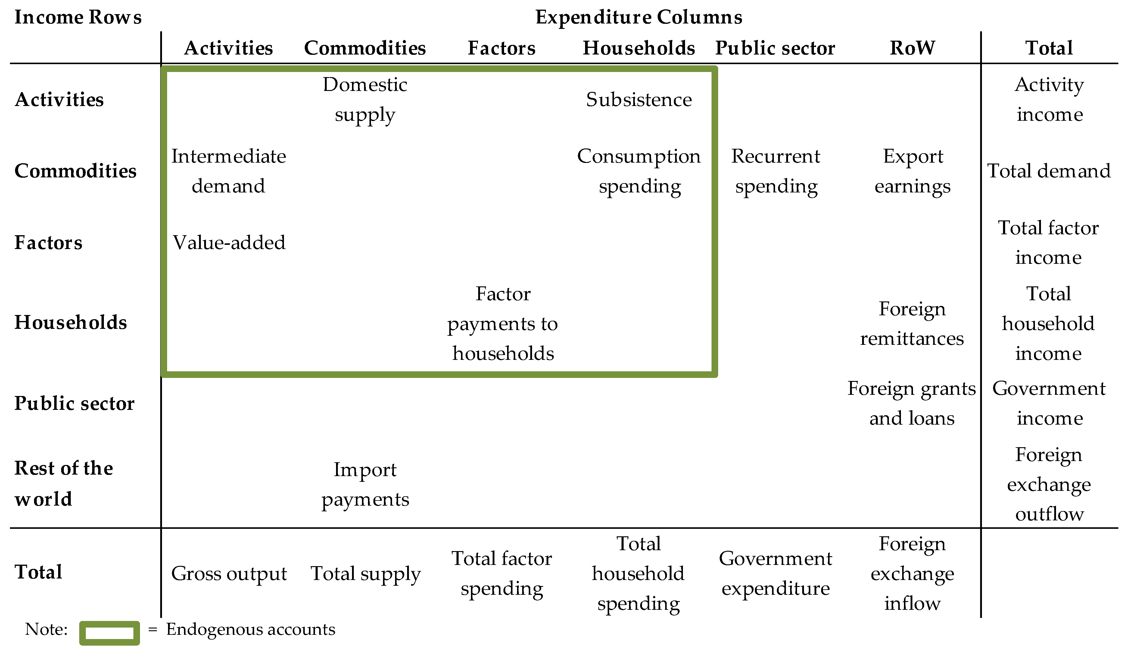
In Kenya, an increased urban demand for AIVs has led to the increased production of these crops in rural and peri-urban areas [6]. This situation is an “exogenous, demand-side shock” and has direct and indirect effects on the regional economy where those AIVs are produced [6,50]. If the demand for a specific product increases and the capacity for production is available, the production of this good will increase [8,24]. Following this concept, the direct effects are the impacts of an increased AIV demand on the AIV-producing sector itself. Indirect effects are created through linkages between the agricultural sector and other sectors and can be grouped into consumption linkages and forward and backward production linkages (see Figure 1). Backward production linkages are links to other sectors that produce input for the sector’s production activities, while forward production linkages are links to other sectors processing the output of the sector through trade and/or processing [50].
Consumption linkages increase if households have more available money and spend this money on food and goods from inside and outside the region. For example, households could employ their assets like land and labour in AIV production and with this generate higher factor payments to the households resulting in higher household income. The more produce from a household’s own region is consumed, the more the other actors in the regional economy profit from it. Consumption linkages are sometimes the major driver of economic growth in a region [23,51]. Earlier research showed that commercialized AIV production increased the household income of the producing households in certain areas [6,10]. Thus, we expect relatively high consumption linkages for AIV production.
Figure 1.
Conceptual framework of a social accounting matrix (SAM; our own construction based on References [13,50,52]).

Production linkages increase if sectors or crops produce output that can be used for multiple purposes in the village economy [52] or if sectors are linked to many other sectors in the region [53]. Thus, production linkages depend not only on the product produced but also on the agricultural system in which the product is grown. In Zimbabwe, large-scale agriculture has higher multiplier effects on the overall economy than small-scale agriculture and thus better supports economic growth [22]. In rural Vietnam, the cash crops tea and coffee have the highest multiplier effects, as opposed to food crops [23]. The main reason for this is that production systems use relatively large amounts of input such as labour, fertilizer or irrigation. If those are supplied by the sector’s own economy, backward production linkages are higher.
Traditionally, AIVs are grown with relatively little input [54], which suggests relatively few backward production linkages. However, we have seen a trend towards more input-intensive production methods for AIVs in Kenya, especially when farmers supply AIVs to supermarket chains [11,55].
Forward production linkages include the processing and trade of the products [50]. AIVs in Kenya are usually sold fresh in bundles to the end customer, and in rare cases, processing steps such as drying or cutting take place beforehand. Thus, we do not expect many forward production linkages to the AIV sector.
Crops or production systems that create higher multiplier effects on the overall economy through production linkages do not necessarily create the highest income effect on a given target group. While large-scale agriculture and cash crops had the strongest effect on the overall economy in the case of Zambia and rural Vietnam, small-scale agriculture and food crops had the highest direct income effect on poor, rural households [22,23]. In rural Pakistan, the expansion of traditional agriculture significantly benefitted poor, rural farmers but not agricultural labourers and the non-farm poor because of a lack of linkages between the rural farm and non-farm economies [53].
3. Data and Methodology
3.1. Data
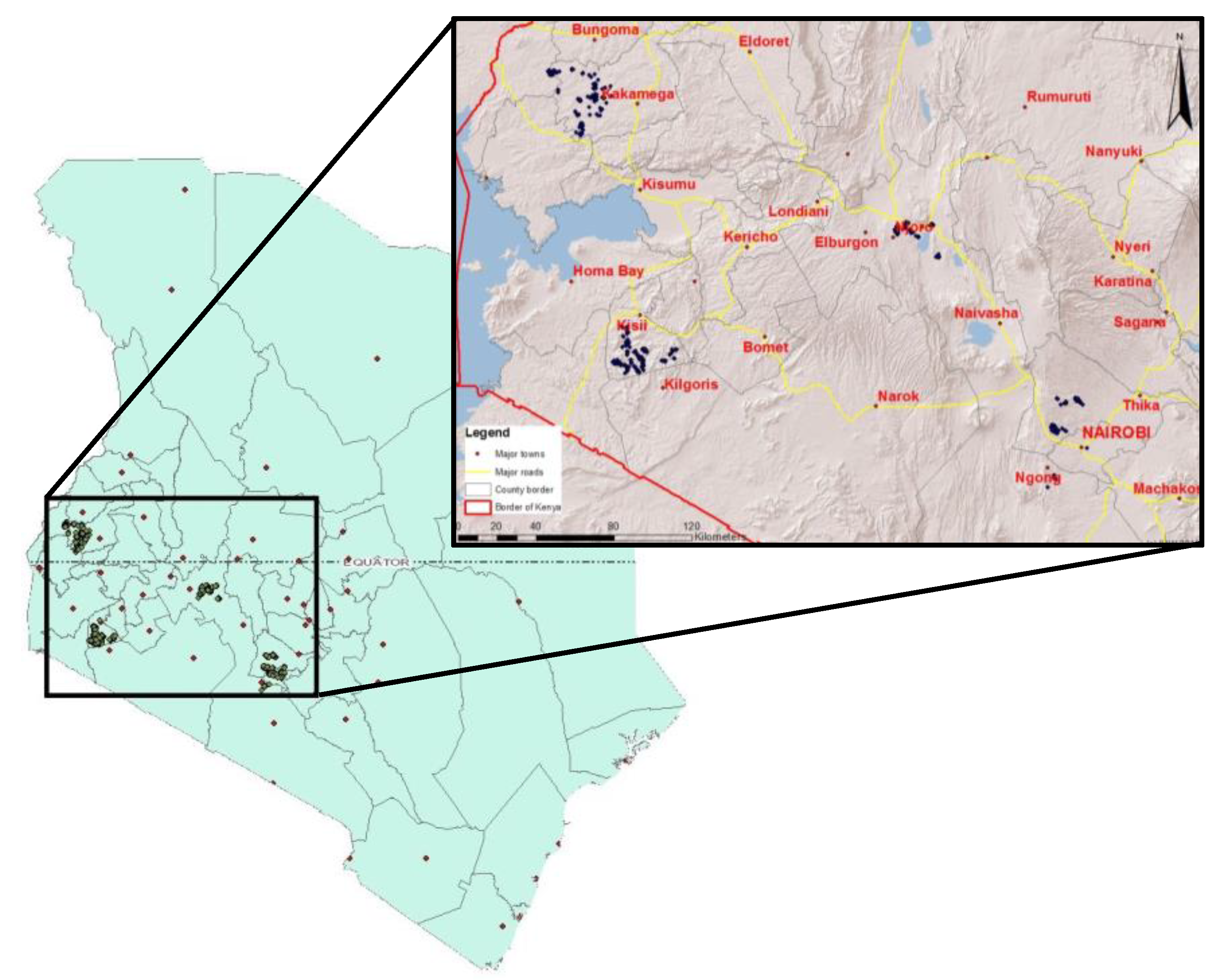
The analysis was based on the HORTINLEA Household Survey 2015 of 706 vegetable producers in Kenya, of which 201 and 202 were interviewed in rural Kakamega and Kisii Counties, respectively. In peri-urban areas in Nakuru and Kiambu Counties, we interviewed 151 and 152 households. The households in Kisii and Kakamega are relatively far from large urban centres and have less available infrastructure than those in Nakuru and Kiambu. Figure A1 in the Appendix shows the geographic sample distribution in Kenya.
The questionnaire covered all farm and off-farm income sources for the household and all food and non-food consumption. Remittances and pension payments to and from the household were included, as well as incomes from savings and costs for loans. Furthermore, the geographic range of buying and selling was included to assess the input and output in the village economy. The HORTLINEA Household Survey 2015 was the second wave of a three-year panel. Data about family labour, which was not covered in detail in the 2015 questionnaire, was derived from the 2014 dataset.
It is important for the design of a SAM to evaluate the level of market integration among the village households [13]. The households in our study area live in villages, where we see an intermediate level of market development, i.e., many activities in the households have a certain level of market orientation, but a large share of the household consumption is generated via subsistence production.
3.2. Methodology
3.2.1. Cluster Analysis
Institutions in the context of village SAMs are economic actors that behave the same if they belong to the same category [13]. In our case, the economic actors were the households living in the area, which we grouped according to geographic distribution and food security at the household level using a cluster analysis.
First, we separated rural and peri-urban households using a dummy because of the substantial differences between public infrastructure and income in rural and peri-urban Kenya. Second, we used a two-step cluster analysis following previously published methods [56], in which the dataset was first pre-clustered, and final clusters were then generated through hierarchical clustering. This technique is suitable to analyse large datasets and was thus useful in this case [56]. We used the Bayesian information criterion to determine the best number of clusters [57].
To determine the food security status of the households, we included several food security indicators at the household level in the cluster analysis. The choice of indicators was guided by the four following dimensions of food security [29]: availability, access to food, the utilization of food and the stability of the first three dimensions. The first dimension—availability—could only be influenced and measured at national and regional levels and was thus not addressed in the cluster analysis on household level. An overview of the food security indicators used for the cluster analysis can be found in Table 1.
The access dimension describes the household’s physical access to food. The available per capita income is one key indicator for this food security dimension [29]. The World Food Program (WFP) Food Consumption Score (FCS) [58] is also a good food security indicator for the access dimension because it correlates well with the caloric intake of the household members [59]. To further address the complexity of food security, we included the Coping Strategy Index (CSI) as an indicator in the cluster analysis. The CSI assesses food insecurity via the behaviours shown by a household related to food procurement over the course of a year and indicates the level of food access in the household [60]. The utilization dimension captures the nutrient content of the food and how the body makes use of those nutrients. Thus, aspects such as sanitation and health also play a role. If individuals have diarrhoea, for example, their uptake of micronutrients is severely impaired, potentially leading to micronutrient deficiencies [61]. Because of its complexity, two indicators were taken into account in the utilization dimension: the Household Dietary Diversity Score (HDDS), which was correlated with the occurrence of diseases related to micronutrient deficiency [62], and the number of days that household members missed work or school in the previous month due to diarrhoea. The stability dimension shows the stability of the access and utilization dimensions over time. This is indicated by the Months of Adequate Household Food Provisioning (MAHFP) score [63].
3.2.2. Construction the Social Accounting Matrix
The overall design of the SAM and its accounts are discussed in this chapter. Where primary data were missing, we made reasonable assumptions based on secondary literature and the conditions at the study sites. We describe those assumptions in this chapter as well.
Activities
The activity accounts in a SAM showed all possible income and commodity-generating activities, that a household can engage in. They needed to be separated from the commodities they produced because different activities can lead to the same results. For example, meat can be produced by raising livestock or hunting. Agricultural activities were separated by the different crops produced by the household, with one account for livestock. Commodities produced by livestock activities can be meat and edible and non-edible livestock products. As off-farm income activities, we included self-employment, wage employment for unskilled agricultural labour and skilled wage employment in the public and private sector. Furthermore, fishing, hunting, collecting and logging from public sources were included in one activity account, as were firewood and coal production.
Commodities
Commodity accounts showed all products produced by the actors in the village economy in terms of farm gate prices. The output was differentiated according to marketing destination as follows: intermediate products for other activities, subsistence, products produced for the village market and products exported to other regions in Kenya. Products exported to countries outside Kenya were negligible and were thus included in the “Rest of the world” account.
Household food consumption was covered through detailed one-week recall in the survey. This value was then multiplied by 52 to show the annual food consumption. We thus assumed that food consumption did not vary substantially throughout the year and was not affected by seasons. This is indeed a very strong assumption, but we argue that this is a good estimate for two reasons. First, a one-year recall on the availability of major food groups showed that most households eat the same food throughout the year. Second, secondary data suggested that the total annual food consumption in our sample was well within the range of the Kenyan average.
Non-food consumption was captured through one-year recall in our survey. The only exception to this is the energy consumption, which was captured as an average week in the previous year that was multiplied by 52 to determine the annual consumption.
Factors
Factor accounts include all input needed for the activities. Land was separated into land rented by the households and owned land. The value of the owned land was described in terms of the opportunity costs of what they would have had to pay if they were to rent that land. The value of this land rent was derived by the average rent payments for rented land in the county. In cases of household-owned land that was rented to someone else, this was considered income. We did not determine where the persons renting land from the households were living, but the majority of the plots rented out to other people were near the residences. We thus assumed that landlords were part of the village community.
Labour as an input factor was separated into hired labour and family labour. The labour requirements for each crop were taken from the 2014 dataset because they were not determined in the 2015 questionnaire due to time constraints. We argue that the labour requirements were the same for each crop every year. Labour requirements for livestock and sourcing from the public were difficult to capture in our sample. We thus calculated the requirements per animal and per kg of collected goods based on secondary literature and additional expert interviews. The costs for hired labour were considered in the input data for each specific crop. Family labour was valued as the opportunity cost of how much money they would have earned if members of the households had worked as unskilled labourers in the agricultural sector. We used average daily wages for unskilled agricultural labourers in the county from our own data.
The costs for pesticides and inorganic fertilizer were included in our input data for each specific crop, as were the origins of those products. To estimate the quantities of organic fertilizer available to the household, we calculated the household’s total manure production by multiplying the household’s animal headcount with the value of solid waste production per animal per day for each respective kind of animal from secondary data [64,65,66]. Not all of the manure was applied directly to the field. Based on our own field experience, we thus assumed that 70% of the total manure produced was distributed evenly over all plots. Since there is no formal market for manure in Kenya, there is also no price for it. We valued the manure as the opportunity costs involved in buying inorganic fertilizer instead of applying a household’s own manure. The most commonly used fertilizer in Kenya is DAP (diammonium phosphate) [67], which consists of approximately 18% nitrogen and 20% phosphate [68]. DAP was sold at 3200 Kenyan shillings (Kshs) per 50 kg bag in 2015, which is equivalent to a price of 5.65 USD/kg nitrogen and 6.27 USD/kg phosphate.
Determining the income from and expenditure for capital is a challenge in SAM design because the generation of reliable data in household surveys is difficult. During the survey, we determined savings with an approximation question to circumvent underreporting, which is common in this field. Furthermore, we asked for the exact amount of the loans for private and business purposes held by the household. In 2015, the Kenyan government introduced a cap on interest rates for loans and a minimum interest rate for savings [69]. The Central Bank of Kenya issued, on average, loans at an interest rate of 10.5% in 2015 [70], which led to an average loan cap of 14.5% and an average savings interest minimum of 7.35% in 2015. Since law enforcement is still an issue in Kenya, we assumed that all banks used the maximum allowed ranges for loan caps and minimum savings interest. Even if some banks offered cheaper loans, some may still have circumvented the law or simply ignored it. We thus considered those values as costs for and revenue from capital and argue that these are valid approximations of reality. Smallholder farmers in particular often have limited access to formal banking services in Kenya [71], which leads them to borrow from informal money lenders with higher rates than the formal banking sector. In our sample, however, the use of those informal loans was relatively small and thus did not greatly influence the total balance in the SAM.
3.2.3. Multiplier Analysis
To model the effect of the change in demand for AIVs at the farm and village levels, we used a multiplier analysis calculated via the Leontief inverse of the SAM. First, all accounts were classified as endogenous or exogenous. Exogenous accounts are those that the modeler can change; endogenous accounts are determined by the village parameters [13]. In our case, the households in the region, their activities, the commodities they produced and the factors used were endogenous. Government spending, the rest of the region and the rest of Kenya and the world were exogenous (see Figure 1).
Then [13], we first normalized the SAM and generated a multiplier matrix M by calculating the Leontief inverse of the endogenous accounts, A, as follows:
M = (I – A)−1.
The effect, Y, on the regional economy because of a change in exogenous demand, X, was then denoted as follows:
Y = M ∗ X.
Y not only shows the production linkages calculated by the Leontief inverse but also includes the expenditure linkages in the regional economy, thus including the direct and indirect effects of the increase in exogenous demand on the village economy.
4. Results
4.1. Results of the Cluster Analysis
The cluster analysis grouped the data into four different clusters as follows: one food-secure cluster and one food-insecure cluster in rural and peri-urban areas each (Table 2). In general, household income in rural areas was lower than that in peri-urban areas, and a higher share of the households fell into the food-insecure cluster in rural areas than in peri-urban areas. The average annual per capita income was below the national poverty line of 1,535 Purchasing power parity dollars for the year 2015 (PPP$ (2015)) for both the rural household cluster and the food-insecure peri-urban cluster (The last national poverty line published by KNBS was 78,048 Kshs in March 2018. This was adjusted to PPP$ (2015)).
The FCS, which reflects the access dimension of food security, was relatively high in the peri-urban areas regardless of the cluster and lowest in food-insecure rural areas. The cut-off point for the moderately food-insecure households according to FCS was 42, and that for severely food-insecure households was 28 [58]. Thirty-three households in cluster 1 fell under 42 points, as well as 7 and 8 in clusters 2 and 3, respectively. Only four households fell below the threshold of 28 FCS points, and they were situated in rural areas. This shows that the households in our sample were more food-secure than the Kenyan average.
The overall HDDS was in the middle of the scale, showing that even in the food-secure clusters, food variety was an issue. Even the food-secure cluster in peri-urban areas with a mean monthly income of 3000 PPP$ had only an average HDDS of 8.9, while the maximum value was 12. The prevalence of diarrhoea was much higher in the food-insecure clusters, showing that even if the uptake of micronutrients was sufficient for members of the households, their bodies did not make full use of them.
The biggest difference between food-secure and food-insecure households was in the stability dimension. On average, the food-insecure households reported only between 4.1 and 5.5 months per year in which the household head considered the food supply sufficient for the family’s needs.
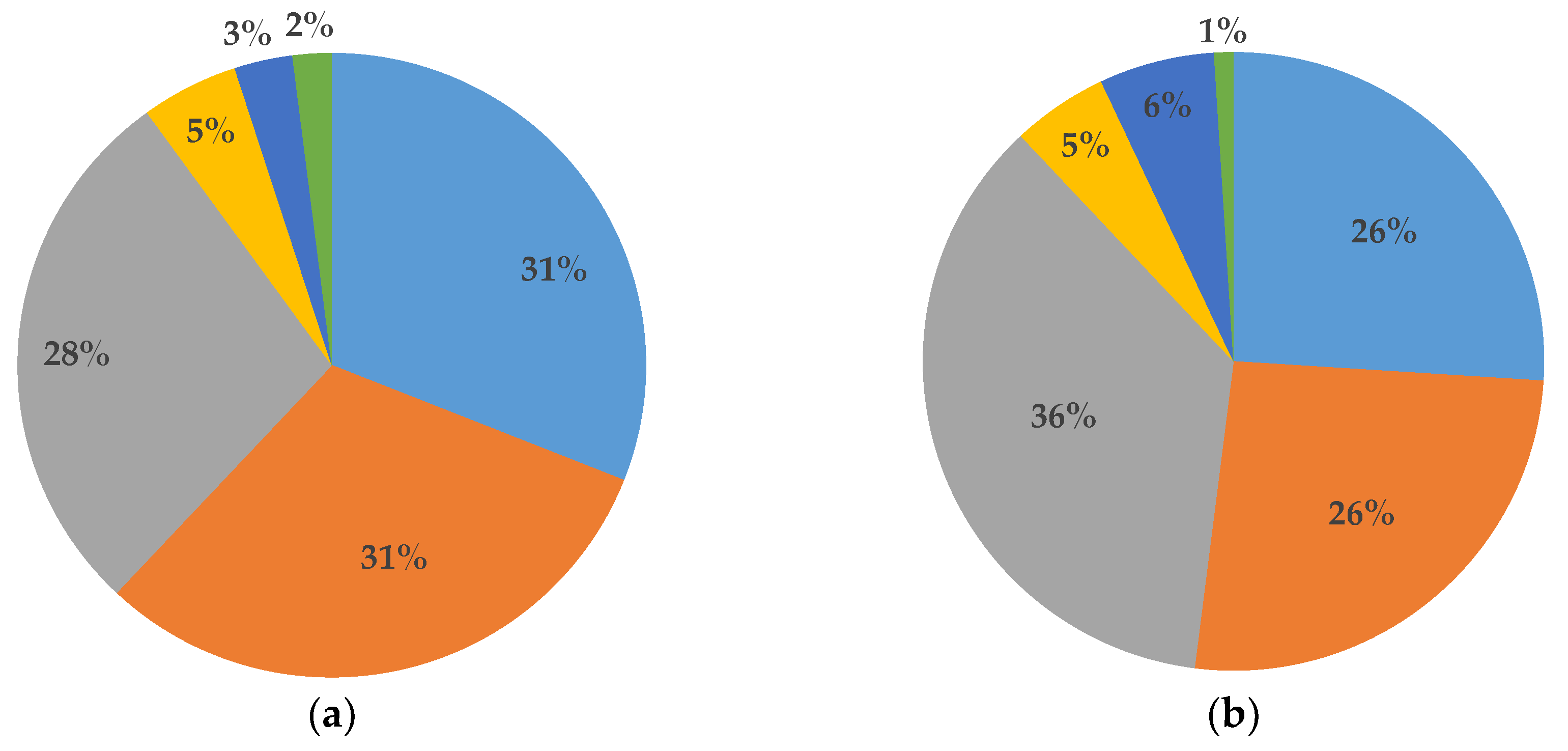
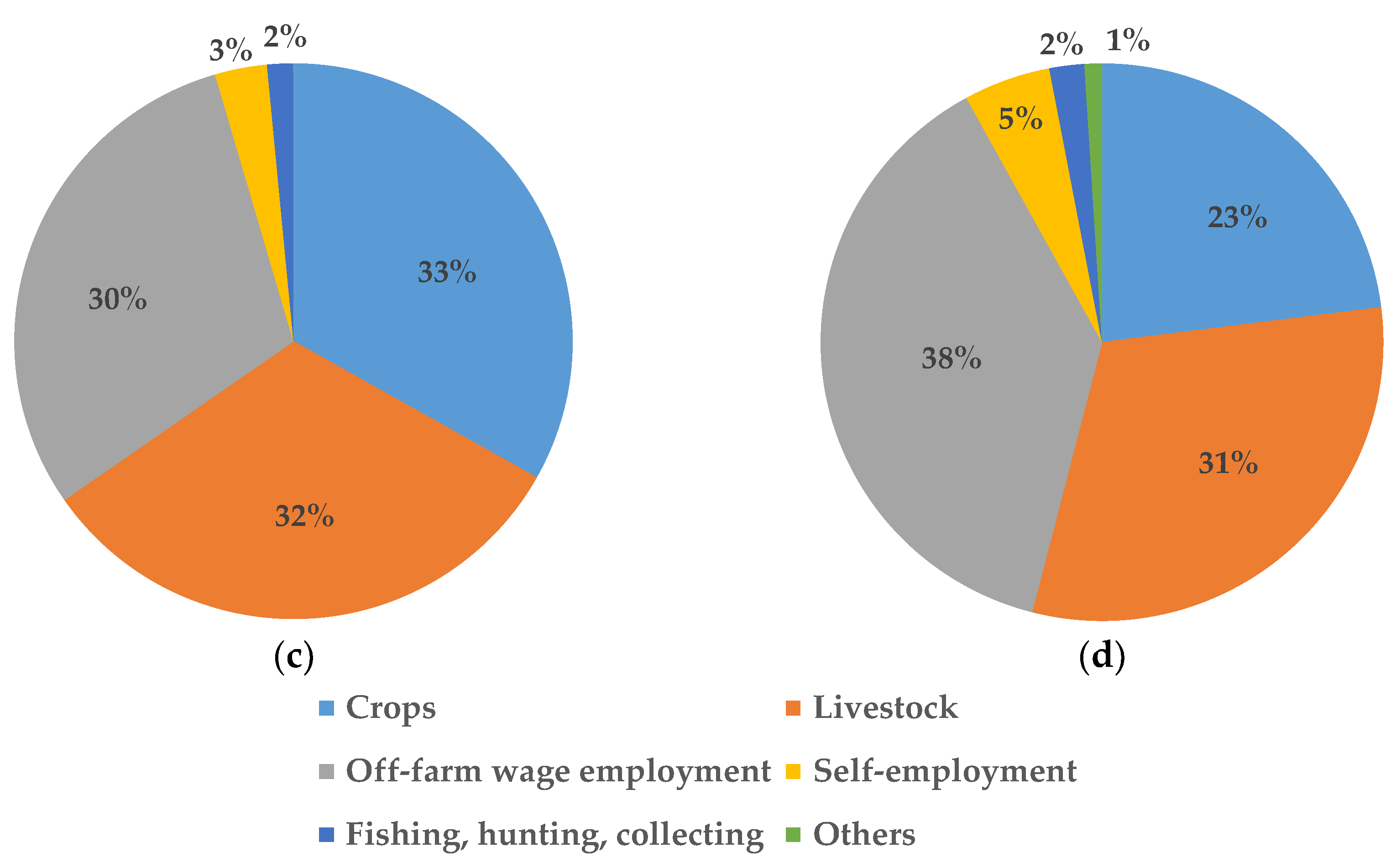
Households from food-secure clusters earned a higher share of their income from off-farm employment and less income from cropping activities than food-insecure households (Figure 2). This was regardless of whether the households were situated in peri-urban or rural areas. Rural households relied more on public resource extraction than peri-urban households. The food-secure rural cluster had the highest proportion of income from this activity, which included firewood extraction, coal production and timber cutting.
4.2. Overview of the SAM
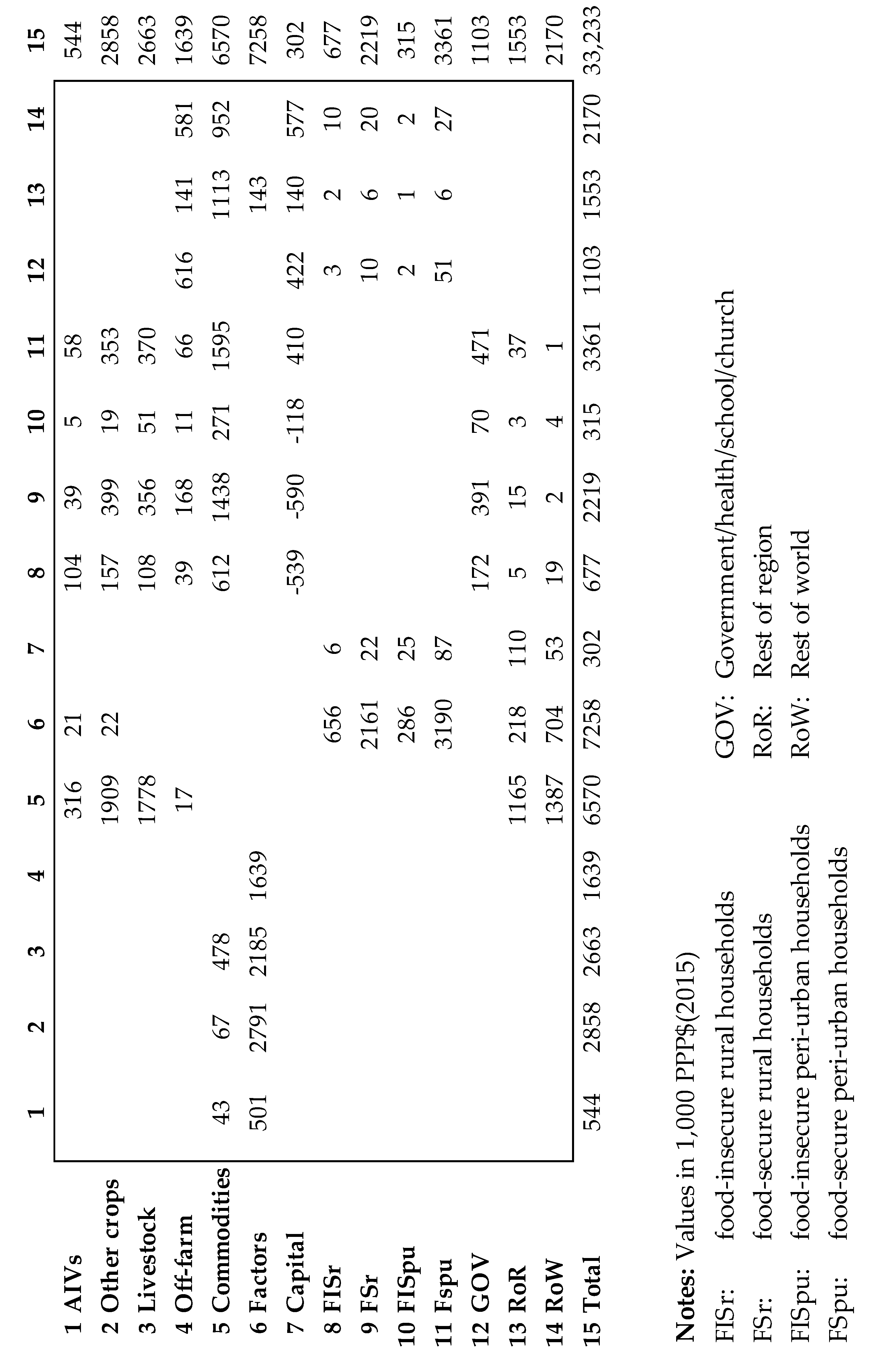
Figure 3 shows the SAM in a condensed form. The fully disaggregated SAM can be found in the supplementary files of this paper (Table S1).
The overall Gross Domestic Product (GDP) calculated at factor cost was 7.1 million. The PPP$ was approximately 1.5 times the value of a representative sample size from the four investigated counties according to the national statistics [72]. This is a very realistic value and shows that the overall economic activities in the study regions were well captured. The GDP of the calculated SAM was higher than that of the official statistics because the official statistics do not include subsistence farming and natural resource extraction. Those activities were covered in our SAM, making the estimated economic activity more accurate but also increasing the calculated GDP.
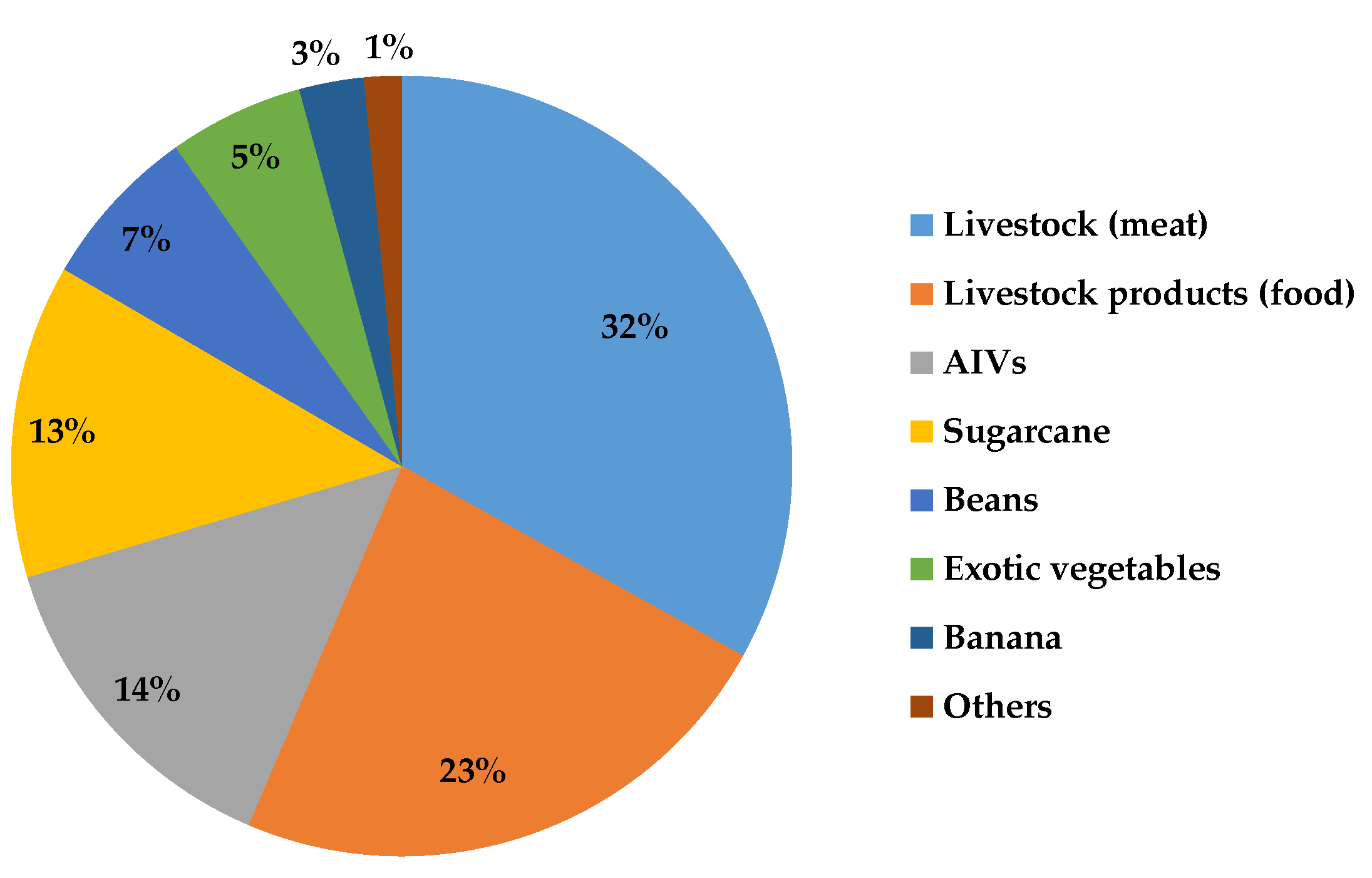
The sample regions were net importers with a total import value of 1.3 million. The PPP$ and the total export value was 0.95 million PPP$. The exports from the sample regions to the rest of Kenya comprised mainly agricultural goods. Livestock and livestock products such as meat, milk and living animals comprised the highest share, followed by sugarcane and AIVs (Figure 4). It is important to note that those shares were based on monetary values. Livestock and livestock products are relatively pricy in Kenya compared to crop products. Thus, with respect to quantities, exports from crops were probably higher than those depicted in this graph. What we can say, however, is that the regions had a self-sufficiency rate above 100% in agricultural products—they produced more agricultural goods than they consumed.
The most recent national SAM from Kenya was less disaggregated in agricultural activities, but the traditional strong role of agricultural activities was visible as well [31]. The most important export crops are coffee, tea and horticultural food crops. In contrast to our sample regions, livestock and livestock products did not play such a substantial role in exports at the national level [31], but this was most likely because those products are mainly consumed in Kenya itself. Thus, exports from of our sample regions were consumed in other parts of Kenya—especially in large cities. Furthermore, the counties we investigated are traditionally strong in the poultry, beef and dairy sector [73].
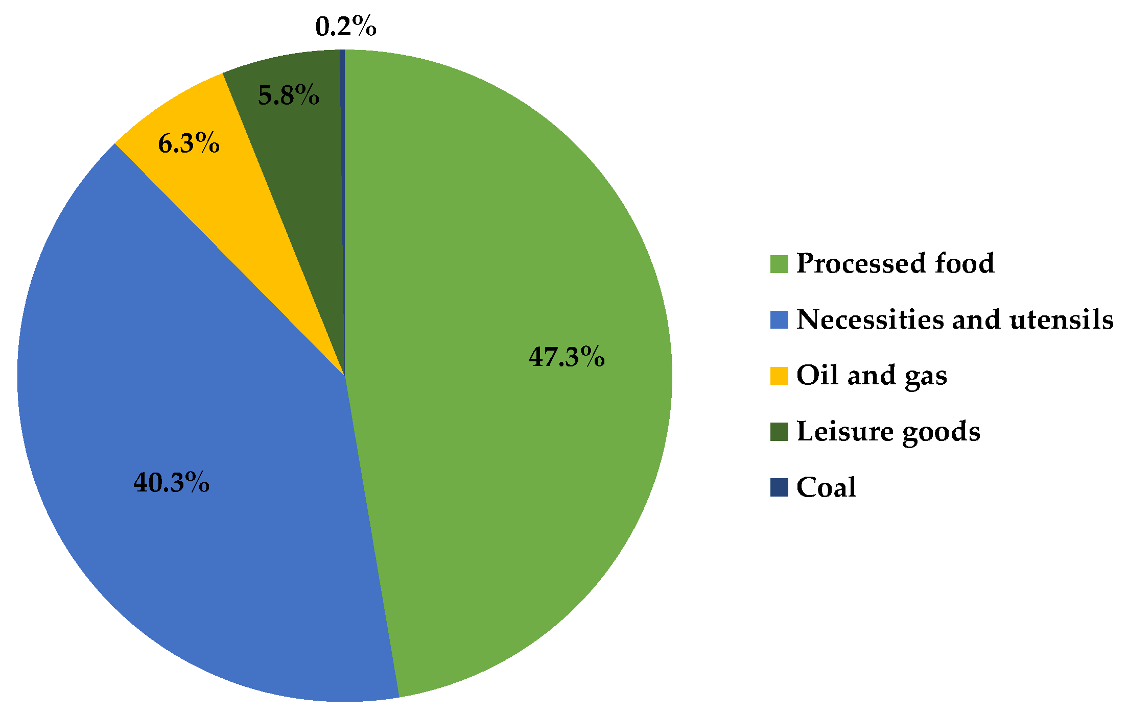
Imports comprised mainly processed foods, necessities and utensils. Processed foods were anything beyond the raw agricultural products—from milled maize to corn flakes.
Examples of necessity goods and utensils are clothes, washing products, building materials and vehicles. Energy in terms of oil and gas also played an important role. The proportion of processed foods and necessities and utensils in the overall import value is slightly lower in reality because our dataset contained little information on the output of off-farm business activities pursued by the sampled households. Those were production as craftsmen or food processing as millers or butchers or in restaurants. Thus, the import shares were taken as a careful estimate that indicated only the direction.
In the overall Kenyan economy, the main imported articles are building materials and clothes, followed by fossil fuels such as gas and coal [31]. Almost 100% of fossil fuels are imported into Kenya. Thus, if we consider potential overestimation due to inaccuracy in data from the processing sector, the import portfolio of our sample region and at the national level were the same (Figure 5).
4.3. Multiplier and Income Effects
Table 3 shows the calculated multiplier effects the selected cropping activities of the sample. Other activities can be found in the Appendix (Table A1). The full multiplier calculation can be found in the supplementary materials (Table S2). The table reads as follows (with bananas as an example): for every increase in demand of one PPP$, we saw an increase in the overall economic activity of 2.115 PPP$. A total of 1.064 PPP$ of this increase came from the sample’s own sector, and 1.051 PPP$ came from the link between the banana sector and other sectors in the economy. Overall, the multiplier values for agricultural activities were in the same range as those in other studies on comparable areas [8,23,52], suggesting a sound estimate.
Horticultural food crops had the highest multiplier effects in the sample regions, with an approximately 2 PPP$ increase in economic output for every PPP$ increase in demand. AIVs were the most prominent group of crops with high multipliers, and of those, the less frequently produced AIVs such as mitoo, jute mallow or enderema (aggregated in the category of other AIVs) exhibited the highest multipliers. Other crops, such as tea, coffee or maize, exhibited lower multipliers, even though they were still approximately 1.8 to 1.9 PPP$ per 1 PPP$ increase in demand.
Households benefit from an increase in demand for specific products through a direct income effect if they produce those products. For all households in our sample, the direct income effect was highest for seldom-produced AIVs, followed by sweet potatoes, bananas and sugarcane (see Table 4). The income effects of other activities can be found in the Appendix (Table A2). Because of their different levels of productivity and available production parameters, each group of households obtained the highest income effects with specific crops. For the least food-secure group in rural areas, those were pumpkins, sugarcane and coffee. Food-secure rural areas profited from sugarcane, bananas, sweet potatoes and the seldom-produced AIVs. In the peri-urban areas, the most important crops were the same for both food security groups: coffee, Irish potatoes and spinach.
5. Discussion
Results of the cluster analysis showed that food security remains a challenge especially in rural areas. As compared to previous studies in Kenya [42,44], we investigated this problem with multiple indicators covering several dimensions of food security [29]. This way it became evident that while households in both areas were food secure according to the availability and access dimension, problems existed in the utilization and stability dimensions.
The sample region is not only self-sufficient in many agricultural products but also exports especially livestock products and horticultural crops to other parts of Kenya (Figure 4). Thus, neither the availability of food in the sample region poses a challenge on food security in the region, nor does the access to food on household level, as the households’ income and FCS show only minor problems.
The HDDS, as indicator for the utilization dimension, captures dietary diversity in the households and correlates with micronutrient deficiencies among household members [62]. The lack of dietary diversity was a problem in both rural and peri-urban areas and was also independent from the income situation of the households. Thus, even if the households have the means to buy or produce sufficiently nutritious food, they refrain from it. Reasons for this could lie in the lack of nutrition education [2] or the lack of supply of safe nutritious foods like vegetables and fruits [44]. Many households in our sample stated that they do not trust the food safety of fresh vegetables bought from the market, because they fear contamination through waste water or improper post-harvest handling. In rural areas, the utilization dimension was also impaired by high rates of diarrhoea among household members. This problem can derive from a lack of infrastructure in investigated areas. The sewage system in rural Kenya is not separated from the fresh water supply, increasing the risk of contamination with bacteria, which can cause diarrhoea. Diarrhoea is problematic especially for the healthy development of children, because even if they have access to all the essential nutrients, their bodies cannot make use of them, causing risks of micronutrient deficiencies.
Another challenge to food security in rural areas is the stability dimension. Households showed relatively low levels of MAHFP, despite being food secure according to FCS and household income. The FCS was measured from the food supply of the previous week, and the annual per capita income was measured for the entire previous year. However, even if those two indicators are sufficiently high, households still face a substantial risk of food insecurity if food availability is linked to seasonal patterns such as harvest times on their own fields or labour demand on other farms.
In the regional economy in our study area, horticultural food crops and especially AIVs have stronger multiplier effects than cash crops like tea or coffee. AIVs are predominately grown as food crops in small-scale agriculture in rural and peri-urban Kenya. Those production systems use very limited technology and require a lot of labour that is mainly supplied by the household family members. Inorganic fertilizers or pesticides are seldom applied due to a lack of capital, and seeds often come from neighbours or from their own production. The AIV production is thus linked very strongly with the regional economy, making many people benefit from a demand increase in AIVs [7,9,19]. Because we included the value of organic fertilizer (dung) and family labour used on the farm, we saw those multiplier effects more clearly than those in SAMs based on official statistics, which do not include these factors [14,15]. Furthermore, cash crops in Kenya, such as coffee, tea or maize, are usually produced with more synthetic fertilizer and certified seeds. Even for the typical smallholder, who was prevalent in our sample, farmers stated that if they apply inorganic fertilizer or buy certified seeds, they do so for their cash crops only. While those inputs increase the productivity of individual plots, they are imported to the region and thus create smaller backward linkages to the crops that use them. This is evident in Table 3, which shows that the small multipliers of cash crops were mainly dedicated to smaller linkage effects to other sectors in the sample regions. To foster economic development of these regions it is important for policy makers to focus on crops that have strong backward linkages and are closely connected to the local economy [7,8].
Own crop production is still a major income source for rural and peri-urban households in Kenya (Figure 2). Next to the multiplier effects fostering economic development in the region, it is important to see if the same crops generate high direct income effects for the producing households as well. Overall, horticultural food crops and especially AIVs induced the highest direct income effects on the households in our sample, even though the picture is not as clear as with the indirect income effects through multipliers. When grouping the households according to their food security status, the crops with highest direct income generation potential do not vary so much along the levels of food security, but more along the regions in which the households reside. Thus, the geographic position of the household and with it, climate and soil conditions played a more important role for the direct income effects.
6. Conclusions
This paper analysed livelihood differences between household groups with different levels of food security in rural and peri-urban Kenya. Further, we calculated direct and indirect income effects of AIVs and other crops with a multiplier analysis using an own regional SAM of the area.
Households in rural areas were more strongly affected by food insecurity than households in peri-urban areas. Our research has confirmed that food security is a very complex phenomena and that it is necessary in empirical research to investigate it with several indicators in order to capture its complexity and to give sound policy advice [2,29]. The largest problems for food-insecure households in our sample were the utilization and stability dimensions. For the utilization dimension, dietary diversity needs to be improved throughout all income groups through nutrition education and increased access to safe and nutritious foods [2,44]. Further, our results suggest that diarrhoea especially in rural areas is still very prevalent and correlates with other food security indicators, showing that sanitary infrastructure investments are still needed in these areas. The stability of food security in rural areas is mainly affected by the volatility in agricultural output and food supply, which would need to be tackled through the provision of irrigation and storage infrastructure, to buffer the seasonality of agricultural production [42].
From an overall economic perspective, it is worthwhile to focus on AIVs and other horticultural food crops in the region. This is because inputs are still mainly produced in the sample regions themselves, and an increase in AIV production thus creates higher multiplier effects in the local economies. Further, increasing the output of AIVs and other horticultural food crops increases the availability of nutrient rich food in the region. It is thus important that policy makers focus on developing AIV production in these areas but ensure that the backward linkages to the local economy are maintained. The production of inputs for AIVs such as seeds and fertilizer should still occur in the same regions where the AIVs are produced.
Especially the less commonly produced AIVs show not only high multiplier but also high income effects for the households from which they are produced, but depending on the location, cash crops such as sugarcane, tea and coffee still have relatively high direct income effects on farmers. Thus, the decision of the individual farmer seeking to maximize his or her household income may not correlate with the crops that give the highest economic development to the region or help to increase availability of nutritious foods for the population. Policy makers need to take this into account when designing support programmes. Farmers need to see the economic potential in AIVs, which are becoming an economically interesting crop in Kenya [6].
However, we need to be careful not to draw too strong conclusions from these results, as multiplier analysis is a static model based on the assumption that prices for products and factors remain constant and that there are no changes in technology [13]. The prices of AIVs would decrease if more producers shifted to producing them. To compensate for this, production needs to become more efficient, and more inputs from outside the region will likely be imported. We have seen this trend in the production of amaranth, cowpeas and African nightshade; after a substantial increase in demand over the previous decade, the usage of certified seeds and inorganic fertilizer was higher in our sample than for other AIVs. Furthermore, keeping prices constant in the analysis creates a certain path dependency, different factor endowments favoured crops already produced by the households at the time of the analysis. A multiplier analysis can be rather considered a snapshot of the local economy. To further analyse the dynamic effects of an increase in the demand of AIVs, including price changes and changes in factor costs, a computable general equilibrium (CGE) model or an agent-based model (ABM) would be useful.
Furthermore, there were some limitations with respect to the data. We used a representative sample of four counties, but for a full picture on the product and financial flows, a household census would be desirable—though very costly. Village and regional SAMs with imperfect markets face the additional challenge of the lack of market prices for some goods, such as family labour or manure used as fertilizer. In this context, so-called “shadow prices” based on opportunity costs often influence resource and factor allocation in households. We determined those shadow prices with reasonable approximations from our own data where possible and cross-checked and complemented them with secondary data. However, shadow prices depend very much on the individual utility function of each individual household and may not be reflected in the market price alone. Further research at the household level is necessary to capture the full picture here.
Food security is a complex phenomenon, which needs to be addressed by a variety of disciplines in research. Our food security indicators are based on primary survey data of the sample regions and thus give a rather accurate picture on the food security status in this year. Nevertheless, food security indicators remain only approximations of the situation at hand and our dataset has a strong focus on the economic performance of the households. To get a more comprehensive view on the food security situation in the region, we suggest the inclusion of anthropometric indicators like weight and height of children and a food diary of the households. A panel of the data set could give more insights into the long-term stability of food availability and access to food among the respective households.
Supplementary Materials
The following are available online at https://www.mdpi.com/2071-1050/11/11/3017/s1, Table S1: Social Accounting Matrix, Table S2: Multiplier Analysis.
Author Contributions
Conceptualization, H.K., A.F. and U.G.; data curation, H.K.; formal analysis, H.K.; funding acquisition, A.F. and U.G.; investigation, H.K.; methodology, H.K. and A.F.; project administration, A.F. and U.G.; resources, U.G.; supervision, A.F. and U.G.; validation, H.K., A.F. and U.G.; visualization, H.K.; writing—original draft, H.K.; writing—review and editing, H.K., A.F. and U.G.
Funding
This research was funded by the German Federal Ministry of Education and Research (BMBF) and co-financed by the German Federal Ministry of Economic Cooperation and Development (BMZ) through the project HORTINLEA (http://www.hortinlea.org/). The views expressed are purely those of the authors and may not under any circumstances be regarded as stating an official position of the BMBF and BMZ. The article processing charge (APC) was funded by the Open Access fund of Leibniz Universität Hannover.
Conflicts of Interest
The authors declare no conflict of interest. The funders had no role in the design of the study; the collection, analyses, or interpretation of data; the writing of the manuscript, or the decision to publish the results.
Appendix A

Table A1.
Multiplier effects of other activities.
| Activity | Total Production | Own Sector | Linkage Production |
|---|---|---|---|
| Hunting, collecting, logging | 2.097 | 1.076 | 1.021 |
| Firewood and coal | 2.097 | 1.007 | 1.090 |
| Wage agr. sector | 2.060 | 1.000 | 1.060 |
| Wage non-agr. sector | 2.060 | 1.000 | 1.060 |
| Own business | 2.060 | 1.000 | 1.060 |
| Livestock | 2.009 | 1.306 | 0.704 |
Source: own data.
Table A2.
Income effects of other activities.
| Induced Income | FIS Rural | FS Rural | FIS Peri-Urban | FS Peri-Urban | |
|---|---|---|---|---|---|
| Activity N | 697 | 146 | 252 | 51 | 248 |
| Firewood and coal | 1.736 | 0.195 | 0.680 | 0.055 | 0.806 |
| Hunting, collecting, logging | 1.736 | 0.195 | 0.679 | 0.056 | 0.806 |
| Wage employment agr. sector | 1.724 | 0.181 | 0.592 | 0.069 | 0.883 |
| Wage employment non-agr. sector | 1.724 | 0.181 | 0.592 | 0.069 | 0.883 |
| Own business activity | 1.724 | 0.181 | 0.592 | 0.069 | 0.883 |
| Livestock | 1.318 | 0.144 | 0.491 | 0.046 | 0.637 |
Source: own data; note: FIS: food-insecure households, FS: food-secure households.
Figure A1.
GPS points of the survey area (in green) and cities and towns (in red). Source: own construction.
Figure A1.
GPS points of the survey area (in green) and cities and towns (in red). Source: own construction.

References
- Muthayya, S.; Rah, J.H.; Sugimoto, J.D.; Roos, F.F.; Kraemer, K.; Black, R.E.; Noor, A.M. The Global Hidden Hunger Indices and Maps: An Advocacy Tool for Action. PLoS ONE 2013, 8, e67860. [Google Scholar] [CrossRef]
- Kamenwa, R. State of Nutrition in Kenya. Presented at the KPA Annual Conference, Kisumu, Kenia, 25–29 April 2017. [Google Scholar]
- FEWS NET. Kenya Food Security Outlook—June 2017 to January 2018; Famine Early Warning Systems Network (FEWS NET): Nairobi, Kenya, 2017. [Google Scholar]
- Msuya, J.M.; Mamiro, P.; Weinberger, K. Iron, Zinc and ß-Carotene Nutrient Potential of Non-Cultivated Indigenous Vegetables in Tanzania. Acta Hortic. 2009, 217–222. [Google Scholar] [CrossRef]
- Weinberger, K.; Msuya, J. Indigenous Vegetables in Tanzania. Significance and Prospects; AVRDC: Shanhua, Taiwan, 2004; ISBN 92-9058-136-0. [Google Scholar]
- Cernansky, R. The rise of Africa’s super vegetables. Nature 2015, 522, 146–148. [Google Scholar] [CrossRef]
- Cazcarro, I.; Duarte, R.; Sánchez Chóliz, J.; Sarasa, C.; Serrano, A. Modelling regional policy scenarios in the agri-food sector: A case study of a Spanish region. Appl. Econ. 2016, 48, 1463–1480. [Google Scholar] [CrossRef]
- Das, I.; Dutta, M.K.; Borbora, S. Rural–urban Linkages for Development of Rural Economy in Assam: A Social Accounting Matrix Approach. Int. J. Rural 2013, 9, 183–208. [Google Scholar] [CrossRef]
- Hyytiä, N. Rural-Urban Multiplier and Policy Effects in Finish Rural Regions: An Inter-Regional Sam Analysis. Eur. Countrys. 2014, 6, 179–201. [Google Scholar] [CrossRef]
- Gotor, E.; Irungu, C. The impact of Bioversity International’s African Leafy Vegetables programme in Kenya. Impact Assess. Proj. Apprais. 2010, 28, 41–55. [Google Scholar] [CrossRef]
- Rao, E.J.O.; Brummer, B.; Qaim, M. Farmer Participation in Supermarket Channels, Production Technology, and Efficiency: The Case of Vegetables in Kenya. Am. J. Agric. Econ. 2012, 94, 891–912. [Google Scholar] [CrossRef] [Green Version]
- Ewbank, R.; Nyang, M.; Webo, C.; Roothaert, R.L. Socio-Economic Assessment of Four MATF Funded Projects. In FARM-Africa Working Papers; June 2007; Available online: www.betuco.be/marketing/Socio-Economic%20Assessment%20of%20Four%20MATF%20Funded%20Projects%20East%20Africa.pdf.
- Taylor, J.E.; Adelman, I. Village Economies. The Design, Estimation, and Use of Villagewide Economic Models; Cambridge University Press: Cambridge, UK, 1996; ISBN 9780521032292. [Google Scholar]
- Ahmed, I.; Socci, C.; Severini, F.; Yasser, Q.R.; Pretaroli, R. Financial Linkages in the Nigerian Economy: An Extended Multisectoral Model on the Social Accounting Matrix. Rev. Urban Reg. Dev. 2018, 30, 89–113. [Google Scholar] [CrossRef]
- Monge, J.J.; Bryant, H.L.; Anderson, D.P. Development of Regional Social Accounting Matrices with Detailed Agricultural Land Rent Data and Improved Value-Added Components for the USA. Econ. Syst. Res. 2014, 26, 486–510. [Google Scholar] [CrossRef]
- Itoh, H. Understanding of economic spillover mechanism by structural path analysis: A case study of interregional social accounting matrix focused on institutional sectors in Japan. Econ. Struct. 2016, 5, 111. [Google Scholar] [CrossRef]
- Gronau, S.; Winter, E. Social Accounting Matrix. A User Manual for Village Economies; No. 636; Leibniz Universität Hannover, Wirtschaftswissenschaftliche Fakultät: Hanover, Germany, 2018. [Google Scholar]
- Martínez de Anguita, P.; Wagner, J.E. Environmental Social Accounting Matrices. Theory and Applications; Routledge: London, UK, 2012; ISBN 0415539838. [Google Scholar]
- Deldoost, M.; Wagner, J.E. A 2004 Social Accounting Matrix for Italy. Int. Bus. Manag. 2016, 10, 1192–1202. [Google Scholar]
- Hyytiä, N. Farm diversification and regional investments: Efficient instruments for the CAP rural development targets in rural regions of Finland? Eur. Rev. Agric. Econ. 2014, 41, 255–277. [Google Scholar] [CrossRef]
- Mansury, Y.; Hara, T. Impact of Organic Food Agritourism on a Small Rural Economy: A Social Accounting Matrix Approach. Ssrn J. 2006. [Google Scholar] [CrossRef] [Green Version]
- Juana, J.S.; Mabugu, R.E. Assessment of Small-Holder Agriculture’s Contribution to the Economy of Zimbabwe: A Social Accounting Matrix Multiplier Analysis. Agrekon 2005, 44, 344–362. [Google Scholar] [CrossRef]
- Breisinger, C.; Ecker, O. Agriculture-led development in rural Vietnam: A decomposed SAM multiplier model. Q. J. Int. Agric. 2006, 45, 231–251. [Google Scholar]
- Nkang, N.M.; Omonona, B.T.; Yusuf, S.A.; Oni, O.A. Simulating the Impact of Exogenous Food Price Shock on Agriculture and the Poor in Nigeria: Results from a Computable General Equilibrium Model. Econ. Anal. Policy 2013, 43, 79–94. [Google Scholar] [CrossRef] [Green Version]
- Elsheikh, O.E.; Elbushra, A.A.; Salih, A.A.A. Economic impacts of changes in wheat’s import tariff on the Sudanese economy. J. Saudi Soc. Agric. Sci. 2015, 14, 68–75. [Google Scholar] [CrossRef]
- Meng, S. Is the agricultural industry spared from the influence of the Australian carbon tax? Agric. Econ. 2015, 46, 125–137. [Google Scholar] [CrossRef]
- Çağatay, S.; Taşdoğan, C.; Özeş, R. Analysing the impact of targeted bio-ethanol blending ratio in Turkey. Bio-Based Appl. Econ. 2017, 6, 209–227. [Google Scholar] [CrossRef]
- Ferede, T.; Ayenew, A.B.; Hanjra, M.A. Agroecology matters: Impacts of climate change on agriculture and its implications for food security in Ethiopia. In Global Food Security: Emerging Issues and Economic Implications; Hanjra, M.A., Ed.; Nova Science Publishers: Hauppauge, NY, USA, 2013; pp. 71–111. ISBN 9781626181922. [Google Scholar]
- FAO. An Introduction to the Basic Concepts of Food Security; Food and Agriculture Organization of the United Nations (FAO): Rome, Italy, 2008. [Google Scholar]
- Harrigan, F.; McGregor, P.G. Neoclassical and Keynesian Perspectives on the Regional Macro-Economy: A Computable General Equilibrium Approach. J. Reg. Sci. 1989, 29, 555–573. [Google Scholar] [CrossRef]
- Randriamamonjy, J.; Thurlow, J. 2013 Social Accounting Matrix for Kenya. A Nexus Project SAM; International Food Policy Research Institute: Washington, DC, USA, 2017. [Google Scholar]
- Omolo, M.W.O. Construction of a Social Accounting Matrix for Kenya 2009; AGRODEP Data Report No. 4; International Food Policy Research Institute: Nairobi, Kenya, 2014. [Google Scholar]
- Akinboade, O.A. Kenya, agricultural policy options and the poor: A computable general equilibrium analysis. Dev. S. Afr. 1996, 13, 663–680. [Google Scholar] [CrossRef]
- Kiringai, J.; Thurlow, J.; Wanjala, B. A 2003 Social Accounting Matrix for Kenya; Kenya Institute for Public Policy Research and Analysis: Nairobi, Kenya; International Food Policy Research Institute: Washington, DC, USA, 2006. [Google Scholar]
- Mbhenyane, X.; Venter, C.; Vorster, H.; Steyn, S. Nutrient intake and consumption of indigenous foods among college students in Limpopo Province. S. Afr. J. Clin. Nutr. 2016, 18, 32–38. [Google Scholar] [CrossRef]
- Croft, M.M.; Marshall, M.I.; Weller, S.C. Consumers’ preference for quality in three African indigenous vegetables in Western Kenya. J. Agric. Econ. Dev. 2014, 3, 67–77. [Google Scholar]
- Mbugua, G.W.; Gitonga, L.; Ndungu, B.; Gatambia, E.; Manyeki, L.; Karoga, J. African Indigenous Vegetables and Farmer-Preferences in Central Kenya. Acta Hortic. 2011, 479–485. [Google Scholar] [CrossRef]
- Abukutsa-Onyango, M.O. African Indigenous Vegetables in Kenya. Strategic Repositioning in the Horticultural Sector; Jomo Kenyatta University of Agriculture and Technology: Nairobi, Kenya, 2010. [Google Scholar]
- Ndenga, E.A.; Achigan-Dako, E.G.; Mbugua, G.; Maye, D.; Ojanji, W. Agricultural Diversification with Indigenous Vegetables for Cash Cropping and Nutrition: Examples from Rift Valley and Central Provinces in Kenya. Acta Hortic. 2013, 549–558. [Google Scholar] [CrossRef]
- Weinberger, K.; Pichop, G.N. Marketing of African Indigenous Vegetables along Urban and Peri-Urban Supply Chains in Sub-Saharan Africa. In African Indigenous Vegetables in Urban Agriculture; Shackleton, C.M., Pasquini, M., Drescher, A.W., Eds.; Earthscan: London, UK; Sterling, VA, USA, 2009; pp. 225–244. ISBN 9781844077151. [Google Scholar]
- Mwaura, S.N.; Muluvi, A.S.; Mathenge, M.K. African Leafy Vegetables and Household Wellbeing in Kenya: A Disaggregation by Gender. In Proceedings of the 4th International Conference of the African Association of Agricultural Economists, Hammamet, Tunisia, 22–25 September 2013. [Google Scholar]
- Coughlan de Perez, E.; van Aalst, M.; Choularton, R.; van den Hurk, B.; Mason, S.; Nissan, H.; Schwager, S. From rain to famine: Assessing the utility of rainfall observations and seasonal forecasts to anticipate food insecurity in East Africa. Food Sec. 2019, 11, 57–68. [Google Scholar] [CrossRef]
- WHO. The Double Burden of Malnutrition. Policy Brief; WHO: Geneva, Switzerland, 2017. [Google Scholar]
- Momanyi, D.K.; Owino, W.O.; Makokha, A.; Evang, E.; Tsige, H.; Krawinkel, M. Gaps in food security, food consumption and malnutrition in households residing along the baobab belt in Kenya. Nutr. Food Sci. 2019, 138, 47. [Google Scholar] [CrossRef]
- Kamga, R.T.; Kouamé, C.; Atangana, A.R.; Chagomoka, T.; Ndango, R. Nutritional Evaluation of Five African Indigenous Vegetables. J. Hortic. Res. 2013, 21, 99–106. [Google Scholar] [CrossRef]
- Faber, M.; van Jaarsveld, P.J.; Laubscher, R. The contribution of dark-green leafy vegetables to total micronutrient intake of two- to five-year-old children in a rural setting. WSA 2009, 33. [Google Scholar] [CrossRef]
- Legwaila, G.M.; Mojeremane, W.; Madisa, M.E.; Mmolotsi, R.M.; Rampart, M. Potential of traditional food plants in rural household food security in Botswana. J. Hortic. For. 2011, 3, 171–177. [Google Scholar]
- Singh, S.; Singh, D.R.; Singh, L.B.; Chand, S.; Roy, S.D. Indigenous Vegetables for Food and Nutritional Security in Andaman and Nicobar Islands, India. Int. J. Agric. Food Sci. Technol. 2013, 4, 503–512. [Google Scholar]
- Modi, M.; Modi, A.; Hendriks, S. Potential role for wild vegetables in household food security: A preliminary case study in Kwazulu-Natal, South Africa. Afr. J. Food Agric. Nutr. Dev. 2006, 6. [Google Scholar] [CrossRef]
- Breisinger, C.; Thomas, M.; Thurlow, J. Social Accounting Matrices and Multiplier Analysis an Introduction with Exercises. Food Security in Practice Technical Guide 5; International Food Policy Research Institute: Washington, DC, USA, 2009. [Google Scholar]
- Davies, S.; Davey, J. A Regional Multiplier Approach to Estimating the Impact of Cash Transfers on the Market: The Case of Cash Transfers in Rural Malawi. Dev. Policy Rev. 2008, 26, 91–111. [Google Scholar] [CrossRef]
- Faße, A.; Winter, E.; Grote, U. Bioenergy and rural development: The role of agroforestry in a Tanzanian village economy. Ecol. Econ. 2014, 106, 155–166. [Google Scholar] [CrossRef]
- Dorosh, P.; Niazi, M.K.; Nazli, H. Distributional Impacts of Agricultural Growth in Pakistan: A Multiplier Analysis. PDR 2003, 42, 249–275. [Google Scholar] [CrossRef]
- Ayodele, V.I.; Makaleka, M.B.; Chaminuka, P.; Nchabeleng, L.M. Potential Role of Indigenous Vegetable Production in Household Food Security: A Case Study in the Limpopo Province of South Africa. Acta Hortic. 2011, 447–453. [Google Scholar] [CrossRef]
- Neven, D.; Odera, M.M.; Reardon, T.; Wang, H. Kenyan Supermarkets, Emerging Middle-Class Horticultural Farmers, and Employment Impacts on the Rural Poor. World Dev. 2009, 37, 1802–1811. [Google Scholar] [CrossRef]
- Chiu, T.; Fang, D.; Chen, J.; Wang, Y.; Jeris, C. A robust and scalable clustering algorithm for mixed type attributes in large database environment. In Proceedings of the Seventh ACM SIGKDD International Conference on Knowledge Discovery and Data Mining, San Francisco, CA, USA, 26–29 August 2001; Provost, F., Ed.; ACM: New York, NY, USA, 2001; pp. 263–268, ISBN 158113391X. [Google Scholar]
- Hahmann, M. Feedback-Driven Data. Clustering. Dissertation, Technische Universität Dresden, Dresden, Germany, 2014. [Google Scholar]
- WFP. Food Consumption Analysis—Calculation and Use of the Food Consumption Score in Food Security Analysis; WFP: Rome, Italy, 2008. [Google Scholar]
- Lovon, M.; Mathiassen, A. Are the World Food Programme’s food consumption groups a good proxy for energy deficiency? Food Sec. 2014, 6, 461–470. [Google Scholar] [CrossRef]
- Maxwell, D.; Caldwell, R. The Coping Strategies Index—Field Methods Manual, 2nd ed.; CARE: Geneva, Switzerland, 2008. [Google Scholar]
- Gorospe, E.C.; Oxentenko, A.S. Nutritional consequences of chronic diarrhoea. Best Pract. Res. Clin. Gastroenterol. 2012, 26, 663–675. [Google Scholar] [CrossRef] [PubMed]
- Hatløy, A.; Hallund, J.; Diarra, M.M.; Oshaug, A. Food variety, socioeconomic status and nutritional status in urban and rural areas in Koutiala (Mali). PHN 2000, 3, 57. [Google Scholar] [CrossRef]
- Coates, J. Build it back better: Deconstructing food security for improved measurement and action. Glob. Food Secur. 2013, 2, 188–194. [Google Scholar] [CrossRef]
- Barker, J.C.; Hodges, S.C.; Walls, F.R. Livestock Manure Production Rates and Nutrient Content; North Carolina Agricultural Chemicals Manual; NC State University: Raleigh, NC, USA, 2002. [Google Scholar]
- Kirigia, A.; Njoka, J.T.; Kinyua, P.I.D.; Young, T.P. Characterizations of livestock manure market and the income contribution of manure trade in Mukogodo, Laikipia, Kenya. Afr. J. Agric. Res. 2013, 8, 5864–5871. [Google Scholar]
- Snijders, P.; Onduru, D.; Wouters, B.; Gachimbi, L.; Zake, J.; Ebanyat, P.; Ergano, K.; Abduke, M.; van Keulen, H. Cattle Manure Management in East Africa: Review of Manure Quality and Nutrient Losses and Scenarios for Cattle and Manure Management; Wageningen UR Livestock Research: Wageningen, The Netherlands, 2009. [Google Scholar]
- Yamano, T.; Arai, A. Fertilizer Policies, Price, and Application in East Africa; GRIPS Discussion Paper 10-24; Springer: Dordrecht, The Netherlands, 2010. [Google Scholar]
- Mosaic. Diammonium Phosphate. 2019. Available online: https://www.cropnutrition.com/diammonium-phosphate (accessed on 23 March 2019).
- Suri, T.; Bhattacharya, K. Dilemma of Capping Bank Interest Rates in Kenya. 2016. Available online: https://www.businessdailyafrica.com/analysis/Dilemma-of-capping-bank-interest-rates-in-Kenya/539548-3369400-8s5r6j/index.html (accessed on 23 March 2019).
- Trading Economics. Kenya Interest Rate. Available online: https://tradingeconomics.com/kenya/interest-rate (accessed on 23 March 2019).
- AGRA FISFAP. Assessment of Financial Services Landscape for Smallholder Farmers in Ghana, Kenya and Tanzania; Final report; Alliance for a Green Revolution in Africa: Nairobi, Kenya, 2015. [Google Scholar]
- Bundervoet, T.; Maiyo, L.; Sanghi, A. Bright Lights, Big Cities. Measuring National and Subnational Economic Growth in Africa from Outer Space, with an Application to Kenya and Rwanda; The World Bank: Washington, DC, USA, 2015. [Google Scholar]
- FAO; AGAL. Livestock Sector Brief—Kenya; FAO: Rome, Italy, 2005. [Google Scholar]
Figure 2.
Distribution of the income sources by cluster (source: own data). Notes: (a) food-insecure rural cluster (b) food-secure rural cluster (c) food-insecure peri-urban cluster (d) food-secure peri-urban cluster.
Figure 2.
Distribution of the income sources by cluster (source: own data). Notes: (a) food-insecure rural cluster (b) food-secure rural cluster (c) food-insecure peri-urban cluster (d) food-secure peri-urban cluster.


Figure 3.
Overview of the SAM (source: own construction).

Figure 4.
Total exports from the sample region in purchasing power parity dollar for 2015(PPP$ (2015)) (source: own data).
Figure 4.
Total exports from the sample region in purchasing power parity dollar for 2015(PPP$ (2015)) (source: own data).

Figure 5.
Total imports into the sample region in in purchasing power parity dollar for 2015(PPP$ (2015)) (source: own data).
Figure 5.
Total imports into the sample region in in purchasing power parity dollar for 2015(PPP$ (2015)) (source: own data).

Table 1.
Food security indicators used in the cluster analysis.
| Food Security Dimension | Variable | Description | Mean (SD) | Min/ Max |
|---|---|---|---|---|
| Access | hhinc_pc | Annual HH income per capita (PPP$ (2015)) | 1480 (1921) | −51/ 12,973 |
| FCS | Food Consumption Score | 70.35 (15.86) | 26.00/ 112.00 | |
| CSI | Coping Strategy Index | 20.26 (24.32) | 0.00/ 154.97 | |
| Utilization | HDDS | Household Dietary Diversity Score | 8.88 (1.47) | 5.00/ 11.00 |
| Days_missed | Total number of days HH members missed work/school because of stomach ache/diarrhoea | 1.25 (4.52) | 0.00/ 30.00 | |
| Stability | MAHFP | Months of Adequate Household Food Provisioning | 9.42 (3.91) | 0.00/ 12.00 |
Source: own data; notes: HH = household, SD = standard deviation.
Table 2.
Levels of food insecurity in four clusters in peri-urban and rural areas.
| Cluster | 1. Food-Insecure Rural | 2. Food-Secure Rural | 3. Food-Insecure Peri-Urban | 4. Food-Secure Peri-Urban | Total |
|---|---|---|---|---|---|
| N | 146 | 252 | 51 | 248 | 697 |
| hhinc per capita | 751 4 | 1253 4 | 1514 4 | 3079 1,2,3 | 1817 |
| (988) | (1126) | (1569) | (3093) | (2271) | |
| FCS | 52.39 2,3,4 | 69.31 1,3,4 | 67.61 1,2,4 | 74.89 1,2,3 | 67.63 |
| (18.70) | (12.96) | (19.76) | (12.78) | (16.97) | |
| CSI | 31.75 2,3,4 | 13.63 1,4 | 25.14 1,4 | 5.87 1,2,3 | 15.51 |
| (26.99) | (14.58) | (19.49) | (7.96) | (19.36) | |
| HDDS | 6.65 2,3,4 | 8.87 1,3 | 7.53 1,2,4 | 8.88 1,3 | 8.31 |
| (2.28) | (1.41) | (1.95) | (1.32) | (1.88) | |
| Days missed because of diarrhoea | 3.67 2,4 | 0.59 1 | 2.59 4 | 0.24 1,3 | 1.26 |
| (7.83) | (1.75) | (7.42) | (1.38) | (4.52) | |
| MAHFP | 5.50 2,3,4 | 10.54 1,3,4 | 4.16 1,2,4 | 11.68 1,2,3 | 9.42 |
| (4.65) | (1.98) | (4.55) | (0.99) | (3.91) |
Note: Standard error in brackets, n = significantly different from the respective cluster by at least 10%.
Table 3.
Multiplier effects of different cropping activities.
| Activities | Total Production | Own Sector | Linkage Production |
|---|---|---|---|
| Banana | 2.115 | 1.064 | 1.051 |
| Mitoo | 2.105 | 1.001 | 1.104 |
| Pumpkins | 2.104 | 1.002 | 1.102 |
| Other ind. veg. | 2.104 | 1.010 | 1.093 |
| Sweet potatoes | 2.099 | 1.016 | 1.083 |
| Cowpeas | 2.092 | 1.011 | 1.081 |
| Amaranth | 2.066 | 1.012 | 1.054 |
| African night shade | 2.065 | 1.023 | 1.042 |
| Sugarcane | 2.051 | 1.019 | 1.032 |
| Spiderplant | 2.019 | 1.014 | 1.005 |
| Cabbages | 2.017 | 1.005 | 1.012 |
| Kales/Sukuma Wiki | 2.015 | 1.009 | 1.006 |
| Ethiopian kale | 2.006 | 1.003 | 1.003 |
| Spinach | 1.987 | 1.004 | 0.983 |
| Beans | 1.939 | 1.054 | 0.885 |
| Coffee | 1.902 | 1.004 | 0.898 |
| Maize | 1.892 | 1.082 | 0.810 |
| Tea | 1.846 | 1.007 | 0.839 |
| Groundnuts | 1.778 | 1.015 | 0.763 |
| Irish potatoes | 1.759 | 1.007 | 0.752 |
Source: own data.
Table 4.
Income effects of different cropping activities.
| Induced Income | FIS Rural | FS Rural | FIS Peri-Urban | FS Peri-Urban | |
|---|---|---|---|---|---|
| Activities N | 697 | 146 | 252 | 51 | 248 |
| Other ind. veg. | 1.707 | 0.198 | 0.676 | 0.053 | 0.780 |
| Sweet potatoes | 1.703 | 0.205 | 0.682 | 0.051 | 0.764 |
| Banana | 1.698 | 0.197 | 0.668 | 0.053 | 0.780 |
| Sugarcane | 1.605 | 0.212 | 0.673 | 0.043 | 0.677 |
| African night shade | 1.547 | 0.176 | 0.576 | 0.053 | 0.742 |
| Amaranth | 1.538 | 0.171 | 0.555 | 0.056 | 0.756 |
| Spinach | 1.510 | 0.141 | 0.487 | 0.063 | 0.819 |
| Pumpkins | 1.494 | 0.225 | 0.613 | 0.040 | 0.617 |
| Cabbages | 1.483 | 0.154 | 0.502 | 0.058 | 0.770 |
| Mitoo | 1.474 | 0.205 | 0.637 | 0.037 | 0.596 |
| Cowpeas | 1.467 | 0.189 | 0.558 | 0.047 | 0.672 |
| Beans | 1.458 | 0.161 | 0.505 | 0.055 | 0.737 |
| Coffee | 1.455 | 0.117 | 0.374 | 0.073 | 0.891 |
| Ethiopian kale | 1.407 | 0.161 | 0.516 | 0.049 | 0.680 |
| Spiderplant | 1.390 | 0.147 | 0.463 | 0.055 | 0.724 |
| Maize | 1.377 | 0.160 | 0.472 | 0.052 | 0.693 |
| Kales/Sukuma Wiki | 1.374 | 0.146 | 0.471 | 0.053 | 0.704 |
| Tea | 1.218 | 0.219 | 0.544 | 0.023 | 0.432 |
| Irish potatoes | 1.206 | 0.049 | 0.129 | 0.089 | 0.939 |
| Groundnuts | 0.873 | 0.155 | 0.410 | 0.015 | 0.294 |
Source: own data; note: FIS: food-insecure households, FS: food-secure households.
© 2019 by the authors. Licensee MDPI, Basel, Switzerland. This article is an open access article distributed under the terms and conditions of the Creative Commons Attribution (CC BY) license (http://creativecommons.org/licenses/by/4.0/).
Share and Cite
MDPI and ACS Style
Krause, H.; Faße, A.; Grote, U. Nutrient-Dense Crops for Rural and Peri-Urban Smallholders in Kenya—A Regional Social Accounting Approach. Sustainability 2019, 11, 3017. https://doi.org/10.3390/su11113017
AMA Style
Krause H, Faße A, Grote U. Nutrient-Dense Crops for Rural and Peri-Urban Smallholders in Kenya—A Regional Social Accounting Approach. Sustainability. 2019; 11(11):3017. https://doi.org/10.3390/su11113017
Chicago/Turabian StyleKrause, Henning, Anja Faße, and Ulrike Grote. 2019. "Nutrient-Dense Crops for Rural and Peri-Urban Smallholders in Kenya—A Regional Social Accounting Approach" Sustainability 11, no. 11: 3017. https://doi.org/10.3390/su11113017
Note that from the first issue of 2016, this journal uses article numbers instead of page numbers. See further details here.