

Abstract
Much research has examined the sensitivity of tropical terrestrial ecosystems to various environmental drivers. The predictability of tropical vegetation greenness based on sea surface temperatures (SSTs), however, has not been well explored. This study employed fine spatial resolution remotely-sensed Enhanced Vegetation Index (EVI) and SST indices from tropical ocean basins to investigate the predictability of tropical vegetation greenness in response to SSTs and established empirical models with optimal parameters for hindcast predictions. Three evaluation metrics were used to assess the model performance, i.e., correlations between historical observed and predicted values, percentage of correctly predicted signs of EVI anomalies, and percentage of correct signs for extreme EVI anomalies. Our findings reveal that the pan-tropical EVI was tightly connected to the SSTs over tropical ocean basins. The strongest impacts of SSTs on EVI were identified mainly over the arid or semi-arid tropical regions. The spatially-averaged correlation between historical observed and predicted EVI time series was 0.30 with its maximum value reaching up to 0.84. Vegetated areas across South America (25.76%), Africa (33.13%), and Southeast Asia (39.94%) were diagnosed to be associated with significant SST-EVI correlations (p < 0.01). In general, statistical models correctly predicted the sign of EVI anomalies, with their predictability increasing from ∼60% to nearly 100% when EVI was abnormal (anomalies exceeding one standard deviation). These results provide a basis for the prediction of changes in greenness of tropical terrestrial ecosystems at seasonal to intra-seasonal scales. Moreover, the statistics-based observational relationships have the potential to facilitate the benchmarking of Earth System Models regarding their ability to capture the responses of tropical vegetation growth to long-term signals of oceanic forcings.
Export citation and abstract BibTeX RIS

Original content from this work may be used under the terms of the Creative Commons Attribution 3.0 licence. Any further distribution of this work must maintain attribution to the author(s) and the title of the work, journal citation and DOI.
1. Introduction
Tropical vegetation, a key component of the Earth terrestrial ecosystem, plays a pronounced role in land surface budgets of energy, water, and mass, regulating regional and global environmental changes (e.g. Dickinson and Henderson‐Sellers 1988, Cramer et al 2004). Functioning as the most productive biome on Earth and large carbon reservoirs, tropical forests also provide many ecosystem services ranging from improving air quality to sustaining local cultures (Lawrence et al 2005, Delgado-Aguilar et al 2017). Given the vital role of tropical ecosystems in the Earth system, improving the diagnostic and prediction skills of the dynamic variations in tropical vegetation is critical, both scientifically and societally.
Prediction studies have long been applied to numerical weather forecasting (Kukkonen et al 2012). Only until recently, such efforts have begun to emerge in ecosystem dynamics, including the predictions of phenology (Cook et al 2005, Dannenberg et al 2018), crop yield (Hsieh et al 1999, Gonsamo et al 2016), and burned area (Chen et al 2016). However, there have been few studies focused on assessing the predictability and conducting the prediction of tropical vegetation growth.
The driving mechanisms of tropical biotic and abiotic processes are not clearly understood yet, especially on seasonal to longer time scales (Dong et al 2012, Greve et al 2011). Growing attention has focused on identifying the association and causation between climatic variables and tropical vegetation growth. For example, statistical and complex machine learning techniques have been comprehensively utilized to assess the sensitivity of tropical vegetation properties to regional and remote atmospheric conditions (e.g. Zhao et al 2018, Dannenberg et al 2018, Papagiannopoulou et al 2017). These studies, however, have not addressed the predictability of tropical vegetation growth, especially when using sea surface temperatures (SSTs).
SSTs trigger changes in atmospheric modes and determine spatiotemporal patterns of climatic factors such as precipitation, which in turn modulate the variations of tropical terrestrial ecosystems (Wallace and Gutzler 1981). For example, the tropical SST anomalies-induced warm phase of the El-Niño Southern Oscillation (ENSO), also known as El Niño, causes reductions in precipitation over eastern Amazonia by altering the Walker Circulation (Ropelewski and Halpert 1989). The strength of such El Niño events has also been closely related to the inter-annual occurrence of tropical droughts (Dai et al 1997, Lyon 2004, Lyon and Barnston 2005, Gu and Adler 2011). Consequently, these ocean-induced changes have long been recognized to affect tropical ecosystem dynamics in many ways, such as carbon balance (Prentice and Lloyd 1998, Tian et al 1998), water use efficiency (Yang et al 2016), tree mortality (McDowell et al 2018), and occurrence of wildfires (Nepstad et al 1999, Alencar et al 2006, Page et al 2008).
The SSTs also provide relatively longer memory than atmospheric teleconnections and associated changes of specific climatic variables. These are induced mainly by a combination of causes including thermal inertia of the upper ocean, large-scale atmospheric-ocean interactions, and memory of downstream soil moisture (Mei and Wang 2011). Lags in the response of the terrestrial ecosystem to oceanic (namely SST) variations thus make it possible to forecast vegetation changes several months in advance.
Given the substantial indirect influence of SSTs on tropical vegetation growth and their leading role in ocean-atmosphere-biosphere interactions, it is the aim of this study to explore the possibility of predicting tropical vegetation greenness based on SST indices. We will investigate to what degree the monthly changes of tropical vegetation greenness, as characterized by the Moderate Resolution Imaging Spectroradiometer (MODIS) Enhanced Vegetation Index (EVI), can be predicted by SST indices from tropical ocean basins using advanced statistical models.
2. Data and methodology
2.1. Data and data processing
The global monthly time series of MODIS Collection 5 EVI data at 0.05° spatial resolution from February 2000 to December 2013 was derived from Seddon et al (2016). The tropical area between 20 °S and 20 °N was extracted for this study. Land grids with missing values over the entire time series were taken as non-vegetated area and masked out in this analysis. For vegetated grids, we focused only on those with less than 10% missing values (figure S1 is available online at stacks.iop.org/ERC/1/031003/mmedia) and filled these gaps using climatological means to ensure each grid has the same sample size. We de-seasonalized the EVI data, i.e., removed the climatological seasonal cycle at each pixel to produce its monthly anomaly. Linear trends were then removed from the time series to eliminate possible impacts from other factors that are not considered in this study, for example, the CO2 fertilization effect. The detrending treatment also increases the confidence in the correlation analysis by eliminating spurious relationships (e.g. Zhu et al 2017, Gonsamo et al 2016).
We obtained the yearly land use classification map from the MODIS MCD12C1 product at 0.05° spatial resolution from 2001 to 2012, in which land surfaces are classified into 17 categories including natural and human-managed land use types. Fourteen biome classes are present in the tropics, with only 9 of them covering at least 0.5% of the tropical vegetated land surfaces (figure S2). These 9 classes, evergreen broadleaf forest (EBF), open shrub (OSh), woody savanna (WSvn), savanna (Svn), grassland (Gra), wetland (Wet), cropland (Crp), cropland and natural vegetation mosaic (CrpNat), and barren or sparsely vegetated (SV), were thus retained in the subsequent analysis. Since the evolution of biome types from 2001 to 2012 was relatively less pronounced, we assumed that biome classifications have not changed through our study period and the map from 2001 was adopted to aggregate the statistics in this study.
To account for oceanic status, we picked 14 SST indices over 3 tropical ocean basins, namely Niño1 + 2 (far eastern equatorial), Niño3.4 (central equatorial), Niño3 (eastern equatorial), Niño4 (west-central equatorial), and Trans-Niño Index (TNI) from the Pacific Ocean, tropical North Atlantic (TNA), tropical south Atlantic (TSA), North Atlantic tropical (NAT), South Atlantic Tropical (SAT), and tropical Atlantic SST Index (TASI, north-south equatorial SST gradient) from the Atlantic Ocean, and Dipole Mode Index (DMI, west-east equatorial SST gradient), Southeastern Tropical Indian Ocean (SETIO), South Western Indian Ocean (SWIO), and Western Tropical Indian Ocean (WTIO) from the Indian Ocean (figure S3). These indices are monthly SST anomalies calculated relative to the base period of 1982–2005 and averaged over various ocean regions or gradients of two other SST indices. Time series of SST indices were downloaded from the National Oceanic and Atmospheric Administration (NOAA) at http://stateoftheocean.osmc.noaa.gov/all/ and detrended the same way as was EVI.
2.2. Statistical models and evaluation metrics
The coupling strength between oceanic conditions and vegetation growth was first evaluated using linear correlations between the SST indices and EVI anomalies, with the former leading the latter by a number of months ranging from 0 to 11. Pearson correlations were calculated for each combination of SST indices and number of leading months at a grid basis. The maximum absolute correlation coefficient from all combinations was taken as a measure of the impacts of SSTs on vegetation growth. A Student's-t test with a null-hypothesis of zero correlation was used. We restricted our subsequent analysis to those pixels associated with significant (p < 0.01) correlations. The SST index and its corresponding number of leading months associated with the largest absolute correlation coefficient were chosen as the controlling SST index and number of leading months of a certain grid cell.
Given the controlling SST index and its associated number of leading months for a certain grid, we built three predictive models of EVI based on SSTs, namely a univariate linear model (denoted as SST1, y = ax+b), a polynomial model (denoted as SST1p, y = ax2 + bx+c), and a multivariate linear model (denoted as SST2, y = ax1+bx2+c) with the two predictors (SST indices) from two different ocean basins to avoid feature redundancy. In SST1 and SST1p, the controlling SST index as described above was used to construct the models. SST2 was built based on SST1, with the second SST index chosen as the one that minimizes the residual error by adding this index to the SST1 model. Model coefficients (a, b, and c) were obtained from linear least squares fitting.
We used three types of evaluation metrics. The first is anomaly predictability, defined as the correlation between predicted and historical observed EVI anomalies, giving a value ranging from −1 to 1 with higher positive values indicating higher accuracy of the model. It generally measures the similarity of predicted and true values. The aforementioned Student's-t test was also applied to the anomaly predictability. Direction predictability, defined as the proportion of correctly predicted signs of EVI anomalies with values ranging from 0 ∼ 100%, assessed whether the positive/negative sign of EVI anomalies could be correctly predicted. Finally, we further relaxed our requirements by evaluating whether the positive/negative sign of EVI anomalies can be correctly predicted in extreme conditions (referred to as direction predictability in extreme conditions). Extreme value refers to the EVI anomalies at a pixel exceeding one standard deviation. Those pronounced variations of plant growth are especially important for ecological and socioeconomic studies. It is thus important for the statistical models to at least correctly detect the response direction of ecosystem in those extreme conditions.
Each of the three models was run 100 times with unique random divisions of the time series into training (70%) and test (30%) sets for fair evaluation, with the former used to train the model and the latter to evaluate its performance. Models were evaluated based on the evaluation metrics described above, and the median value of the 100 evaluation metrics was calculated over the test set at each grid cell and reported as the model performance in the results. These aforementioned statistics were also aggregated for each biome type to demonstrate the dependence of ocean influences and model performance on individual vegetation types.
3. Results
3.1. Controlling SST index
Of the tropical vegetated grid cells, 92.53%, 95.46%, and 94.69% of South America, Africa, and Southeast Asia, respectively, showed significant (p < 0.01) correlations between a predictor SST index and subsequent EVI anomalies (figures 1(a) and (e)). More specifically, most tropical forest regions were associated with significant correlations, with the area percentages of 88.55% for the Amazon, 88.15% for the Congo, and 90.92% for Southeast Asia. High absolute correlation coefficients were seen mainly over northeastern Brazil, eastern tropical Africa, and northern Australia. These evident connections indicate the potential for SST indices to be successfully applied in the prediction of the dynamics of tropical vegetation growth.
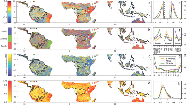
Figure 1. Spatial distributions of (a) the maximum absolute correlation coefficients between EVI and the controlling SST index, (b) the controlling SST index, (c) the number of months with the controlling SST leading EVI responses, and (d) the anomaly predictability with p < 0.05. Only those grid cells with significant correlations between SST index and EVI with p < 0.01 are shown. Grid cells with more than 10% of their EVI time series missing are masked. The rainforest regions are highlighted by polygons in each map. The right column shows the density distributions of (e) correlation coefficients for each region, (f) the same, but for each SST, (g) the number of leading months for all three tropical continents, and (h) anomaly predictability. The line colors denote different continents as indicated in (g). The vertical black lines in (e) and (h) indicate the thresholds beyond which values are significant with p < 0.01 (solid line), 0.05 (dashed line), and 0.1 (dotted line).
Download figure:
Standard image High-resolution imageVegetation growth over tropical South America was influenced mainly by SST from the Atlantic Ocean basin (especially TSA), followed by those from the Indian and Pacific Ocean basins (figures 1(b) and (f), S4). Northeastern Brazil, the region associated with strongest responses of vegetation growth to SST variations, was almost entirely controlled by a unique index, the TSA, with a lead time ranging roughly from 3 to 5 months (figures 1(c) and (g), S5). The positive correlations indicate that an abnormally high temperatures in the tropical South Atlantic favors vegetation growth. Over tropical Africa, DMI from the Indian Ocean and TSA from the Atlantic Ocean exerted notable controls over vegetation growth. For eastern tropical Africa, Niño4 dominated the vegetation growth. Influences from DMI and Niño4 were positive and short in lead time (0–2 months and 3–5 months, respectively). TSA was negatively correlated with EVI over the northeastern Horn of Africa, with TSA leading EVI responses by about 9–11 months. Tropical Pacific SSTs, specifically Niño4 representing the ENSO mode, played a primary role over tropical Southeast Asia and Australia. Over northern Australia, where SSTs pronouncedly influenced vegetation dynamics, tropical Pacific indices (e.g., Niño3.4, Niño3, and Niño4) were negatively correlated with vegetation growth. Tropical Atlantic SSTs (TSA and TNA) also positively controlled some portion of northern Australia. While the responses of vegetation to ENSO indices were short (0–2 months in advance), the optimal forecasting time for TSA/TNA was 9–11 months in advance, probably due to the long distance from the Atlantic Ocean. Actually, it has been shown that the TSA/TNA is partly driven by and thus lags the Pacific Nino index by 3–6 months (Alexander et al 2002), which is consistent with our findings. The longer response time of TSA (9 ∼ 11 months) than that of Niño4 (3 ∼ 5 months) over eastern tropical Africa could also be caused by this relationship between ENSO indices and tropical Atlantic SST indices.
The three specified regions with a strong influence from SSTs on vegetation dynamics are covered mainly by open shrub, woody savanna, savanna, and sparse vegetation (figure S2). The controlling ocean modes varied with biome types but the Niño4, TSA, and DMI were identified as the dominant controlling SST indices (figure 2). No clear controlling indices that overwhelm the rest were seen for other biome types, especially for the cropland, which is a human-managed land use type and thus relatively less responsive to climate conditions. We also did not see a clear dominant controlling ocean mode over the evergreen broadleaf forests either. Such differences in the EVI response to oceanic drivers imply that vegetation adaptation strategies and controlling mechanism of climates vary with biome types.
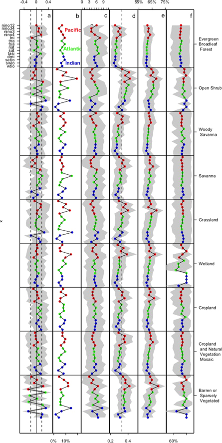
Figure 2. The statistics of (a) the maximum correlation, (b) percentage of area controlled by each SST index, (c) the number of leading months, (d) anomaly predictability, i.e., the correlation coefficient between predicted and historical EVI anomalies, (e) direction predictability (i.e., the percentage of correct predictions in the signs of EVI anomalies), and (f) direction predictability in extreme events (i.e., correctly predicted signs of EVI anomalies when the anomalies exceeding the standard deviation) over different biomes. Abbreviations of biome types are given in Methods. For each biome classification, statistics for each SST index are shown, with the colors representing the ocean basin that a specific SST index belongs to. In (a), (c), (d), (e), and (f), the dotted curve represents the mean value, and the shading area indicates the mean value ± standard deviation. The broken lines in (a) and (d) denote the threshold in the correlation coefficient beyond which the value is significant with p < 0.01.
Download figure:
Standard image High-resolution image3.2. How well can vegetation dynamics be predicted?
Due to the best performance of SST2 among all three statistical models (figures S6, S7, and table S1), we use its results in this section to assess the statistical model's ability to predict vegetation changes. Over the pan tropics, EVI anomalies can be partially predicted by SST (figure 1(d)). Not surprisingly, the highest predictability was determined over the three regions with highest correlations with SSTs as shown in figure 1(a), namely northeastern Brazil, eastern tropical Africa, and northern Australia. The mean anomaly predictability was 0.30 when averaged across the entire tropical vegetated area, with its maximum value reaching up to 0.84. The anomaly predictability is the correlation between historical observed and predicted EVI anomalies, and thus high values, i.e., close to 1, indicate high accuracy of the model. 25.76%, 33.13%, and 39.94% of vegetated areas across South America, Africa, and Southeast Asia, respectively, were associated with significant predictability with p < 0.01. When considering only tropical rainforests, this area proportion dropped substantially to 14.03% for the Amazon, 11.83% for the Congo, and 20.23% for Southeast Asia. The proportion of correctly predicted signs of EVI anomalies (direction predictability) was also examined, and its probability density function (PDF) was distributed to about 60% with a range of about 50%–80% as shown in figure 3(a). The value reached up to about 80% in some places over these three regions that are most responsive to SSTs. We further evaluated whether the model can correctly predict the sign of EVI anomalies when they are abnormally extreme (direction predictability in extreme events), i.e., beyond one standard deviation. PDF of this predictability metric in figure 3(b) peaked at 100%, indicating the high ability of the model to correctly predict the signs for those extremely abnormal EVI values. Though the number of grid cells with extreme EVI occurrences was small (only 2.15% of vegetated grid cells), high predictability above 90% was seen over large proportions of these grid cells primarily over part of eastern tropical Africa (68.25% over South America, 77.34% over Africa, and 66.17% over Southeast Asia). The percentages for the three rainforests were 59.21% (Amazon), 59.80% (Congo), and 61.45% (Southeast Asia). These high percentages indicate that even simple statistical models can correctly predict the direction in vegetation response to extreme events several months in advance, which is the bottom line of developing forecast models.

Figure 3. Density distribution of (a) direction predictability (i.e., the percentage of correctly predicted signs of EVI anomalies) and (b) direction predictability in extreme conditions (i.e., correctly predicted signs of EVI anomalies with the anomalies exceeding a standard deviation) over the three tropical continents.
Download figure:
Standard image High-resolution image
Predictability (in terms of all three-predictability metrics) was higher over open shrub, savanna, grassland, and sparsely vegetated area (figures 2(d)–(f)) than other biome types. Rainforests were associated with the lowest predictability (the EBF) compared with all other 8 biome types that cover at least 0.5% of vegetated area over the tropics. For example, the anomaly predictability was not significant for almost all controlling SST indices except Niño3.4 and Niño4 (with the highest values passed beyond the significant threshold).
4. Discussion
The widely reported strong influence of SSTs on vegetation dynamics over the tropics (e.g. Lyon 2004) indicates a potential predictive skill, which is the focus of this research. Northeastern Brazil, eastern tropical Africa, and north Australia were found to be associated with high predictability of vegetation greenness using SSTs. These three regions are all located in arid or semi-arid climate zones with strong seasonal cycles in precipitation and rainy season(s) of 3–6 months (e.g. Drosdowsky 1993, Nicholls et al 1997, Uvo et al 1998, Yang et al 2015), and are covered mainly by sparse vegetation spanning from open shrublands to savanna.
Anomalies in SSTs drive the changes in atmospheric circulations and consequently modify the spatiotemporal distributions of climate variables (e.g., air temperature, cloud fraction, and precipitation), which then regulate vegetation functioning through plant physiological processes. For example, Philippon et al (2014) showed that ENSO's impacts on Normalized Difference Vegetation Index (NDVI) over eastern tropical Africa occur mainly through its effect on rainfall. Those three regions are recognized as substantially influenced by SSTs and have also been found to be associated with strong coupling between SSTs and local precipitation change in previous studies, suggesting that the climate variable linking ocean status and vegetation responses is primarily precipitation.
Over northeastern Brazil, we found that vegetation growth was almost entirely controlled by tropical South Atlantic SSTs, with higher ocean temperature favoring vegetation growth. The tropical Atlantic meridional SST gradient has long been recognized as a potential influence on the precipitation anomalies over northeastern Brazil (or the Nordeste). For example, Uvo et al (1998) revealed strong positive correlations between south tropical Atlantic SST anomalies and rainy-season precipitation over northeastern Brazil on a monthly time scale in February and especially in April and May. Though the correlation of the contemporary SST anomalies and precipitation is weak in March, SSTs still have a pronounced positive impact on the rainy season precipitation due to their persistent impact that lasts 2–3 months. The region of the south tropical Atlantic basin previously found to exert the impacts is almost identical to the box where the TSA index is defined and calculated (Enfield et al 1999). Giannini et al (2004) further showed that a warmer than normal TSA or colder than normal TNA during the boreal spring (March-May) drives the Atlantic Inter-Tropical Convergence Zone (ITCZ) southward, favoring an early start of the rainy season and a higher accumulated precipitation during the rainy season in the Brazilian Nordeste. The longer response time for vegetation found in our study (3–5 months) compared with 2–3 months found for precipitation by Uvo et al (1998) may result from additional factors including soil moisture memory (Notaro 2008) and plant resilience (Potts et al 2006).
Over eastern tropical Africa, SSTs from all three ocean basins were found to control some area in our study, with DMI and Niño4 imposing positive controls and TSA imposing negative controls. Among the three indices, DMI from the Indian Ocean controlled the largest area of this region. The Indian Ocean SST has been identified as the main driver of precipitation variability over eastern tropical Africa (Goddard and Graham 1999). Specifically, Black et al (2003) indicated that extreme September-October-November precipitation over this region was associated with periods of persistently high DMI, i.e., an anomalous high west-east SST gradient over the tropical Indian Ocean. The variability of seasonal rainfall over eastern tropical Africa is also affected by ENSO (e.g. Giannini et al 2008). Parhi et al (2016) demonstrated that El Niño (quantified by positive values of Niño3.4 in their study) was associated with an increase in the number of wet days and consequently an increase in seasonal mean precipitation. Our findings that tropical Pacific SSTs impose a positive control on eastern tropical African vegetation growth are in line with other studies. Specifically, a positive control of Niño3.4 on the interannual variability in NDVI has been reported (Zhao et al 2018). Similar findings were also shown between ENSO and gross primary production (GPP) on seasonal time scales (Zhu et al 2017). Although the direct relationships between Atlantic SST and precipitation variability over the eastern tropical Africa have not been reported in the literature, to the best of our knowledge these two might be connected through the impacts of TSA on Indian monsoon variability (Kucharski et al 2008) and the subsequent influences of Indian ocean SST on precipitation over TEA (Wang et al 2017).
Over northern Australia, our results indicate that tropical Pacific SST (Niño3.4, Niño3, Niño4) negatively correlates and tropical Atlantic SST (TSA and TNA) positively correlates with vegetation anomalies (both significant with p < 0.01). The negative controls of ENSO on vegetation greenness over this region are consistent with other studies (e.g. Zhao et al 2018). Kirono et al (2010) demonstrated that the seasonal precipitation in northern Australia was best predicted by Niño4 during austral spring and autumn. They also indicated that the summer rainfall over northern Australia can be predicted by Niño4 and the Southern Oscillation Index (SOI). Precipitation over eastern Australia is also well known for its strong response to ENSO mode with the positive phase associated with decreasing precipitation (e.g. Catto et al 2012). Studies have also reported the impacts of Atlantic Ocean SST on Australia rainfall. For example, Lin and Li (2012) identified a positive correlation between tropical Atlantic SST anomalies and rainfall in the northwestern Australia. Though most of the regions in these studies are out of the spatial scope of our research due to the limited spatial coverage in the tropics within 20°S–20°N, these studies provide further insights into ocean influences on northern Australian rainfall.
Vegetation growth over these three semi-arid regions has been indicated as primarily positively controlled by water availability on seasonal (Seddon et al 2016, Papagiannopoulou et al 2017, Green et al 2017) and interannual (Gonsamo et al 2016, Zhao et al 2018) time scales despite differences in statistical methods and temporal ranges of these past studies. As revealed by a rainfall exclusion experiment, not only the rainfall amount but its frequency and timing strongly influence the structure and functioning of semi-arid ecosystems (Miranda et al 2011). Specifically, Barbosa et al (2006) showed that the seasonal variations of NDVI over northeastern Brazil were largely influenced by the seasonal dry and wet periods. They found that greening and browning periods of about 7–8 years coincided with prolonged extreme wet and drought periods, respectively. Over eastern tropical Africa, Hawinkel et al (2016) indicated that the interannual variability in precipitation explained most of the variability in plant growth, particularly over those areas covered by herbaceous plants, with topography and soil playing a limited role. Seddon et al (2016) proposed an explanation for the high plant sensitivity to water availability over northeastern Brazil that indicated the high phenotypic plasticity of leaf senescence and green-up resulted in large amplitudes in the EVI response to drought variability. Green et al (2017) further suggested that the higher fraction of C4 plants in these wet-dry transitional area (Still et al 2003) can explain the higher sensitivity to water limitation since C4 plants also have higher water use efficiency than C3 plants (Ghannoum 2008).
Our results show that oceanic signals substantially contributed to the seasonal and intra-seasonal ecosystem dynamics in the semi-arid regions, and thus can be used to predict ecosystem dynamics in advance. Semi-arid ecosystems have been reported to play a dominant role in the inter-annual variability and trends in global carbon cycle (e.g. Ahlström et al 2015, Poulter et al 2014). This study thus serves as a step forward in our future predictions of global carbon cycles in response to environmental change (Luo et al 2015). In addition, evidence has shown that ecosystem functioning is influenced by variations in hydrological conditions even without changes in mean annual precipitation (e.g. Knapp et al 2002). Our focus on precipitation variability originating from SST variability on seasonal to intra-seasonal time scales thus provides further insights into potential impacts from ongoing anthropogenic climate change.
In contrast to the sparse vegetation located in the semi-arid regions, the lowest predictability of the statistical models was identified over the tropical rainforests, implying non-climatic factors might exert the first-order control of plant growth variability. There is an ongoing debate regarding the driving factors underlying the rainforest growth. Zhao et al (2018) demonstrated significantly positive correlations between NDVI and Photosynthetically Active Radiation (PAR) over the Amazon and Southeast Asia rainforests on interannual time scales. Using Granger Causality technique, Green et al (2017) found that seasonal variations in PAR were responsible for the solar-induced fluorescence (SIF) dynamics over only a very small area in the Amazon with most areas uncontrolled by either PAR or precipitation. Other studies, however, showed no clear climatic control on vegetation variability over the tropical rainforests at seasonal (Papagiannopoulou et al 2017) or interannual (Gonsamo et al 2016) time scales. The dense tropical forests are relatively resilient to climatic variability, which is to a certain extent facilitated by many mechanisms, including their deep roots system that can buffer the drought impacts (Christina et al 2017). In addition, Wu et al (2016) found that leaf development and demography was the primary driver of photosynthetic seasonality in tropical evergreen forests while the seasonality of climate variables played a negligible role. Other factors that may determine the variabilities of tropical forests include wildfires (Van Der Werf et al 2008), availability of soil nutrient (Fisher et al 2012), and deforestation (Hansen et al 2013). The possible major role of these non-climatic factors could explain the lowest predictability of rainforest growth using SSTs as seen in our study. However, our findings that vegetation growth of tropical rainforests is poorly predicted using SSTs do not necessarily apply to other aspects of ecosystem functioning. In contrast, Chen et al (2016) demonstrated that SSTs were good predictors of burned areas over various tropical rainforest regions, including southwestern, eastern, and southeastern Amazon and almost the entire Southeast Asia rainforest. More efforts are thus needed to explore the possibility of predicting growth variation in tropical rainforests.
Behavior of oceanic modes is not completely independent, and interactions among them have been previously reported. For example, Uvo et al (1998) found that the tropical Pacific SST anomaly pattern was well correlated with that of the northern tropical Atlantic, with the temporal correlation coefficient reaching up to 0.8. They also demonstrated that tropical Pacific SST anomalies in winter trigger tropical Indian SST anomalies in spring. Dannenberg et al (2018) revealed that the inclusion of interaction of teleconnections on vegetation phenology improved model accuracy over North American land surfaces. One limitation of our study may thus stem from our lack of consideration of the interactive impacts of different ocean modes on vegetation growth. The resulting potential uncertainties might be the overestimation or underestimation of effects and predictability from the additive sum of a combination of multiple SST indices. Specifically, in our SST2 model, i.e. a linear model with contributions from two additive terms (SST indices), the actual total effects of the two SST indices might be greater or lesser than the sum of them depending on the coefficient of the interaction term.
The selection of model forms, for example, the model complexity, is also expected to highly influence our predictability abilities and may introduce uncertainties. We built three statistical models and compared their performance in figure S6. Based on the median predictability from 100 runs of all three models, SST2 was significantly more accurate than SST1 and SST1p, and SST1p was significantly more accurate than SST1. A Student's-t test between each combination of two models (table S1) confirms that more complex models are always more significantly accurate than the less complex ones, in terms of the median predictability. Further comparisons in the three continents show similar order of the models' accuracy (figure S7). These comparisons indicate that more complex models bring in higher predictability in vegetation responses.
5. Conclusions
Three tropical regions, namely northeastern Brazil, eastern tropical Africa, and northern Australia, that are located in arid or semi-arid climate zones and covered mainly by sparse vegetation including open shrub, were found to be associated with evident influences of SSTs on vegetation growth and consequently high ecological predictability on seasonal to intra-seasonal time scales. Over the tropical rainforests, however, the weakest oceanic influences and thus lowest predictability were identified. The developed statistical models partially predicted the EVI dynamics based on selected SST indices over the pan tropics with limitations owing to the impacts from factors other than climate and model simplicity. As a future direction, more sophisticated statistical models will be tested. We will also evaluate the reliability of the statistics-based model for extracting key oceanic impacts on tropical terrestrial ecosystem production using dynamic experiments with an Earth system model, for example those from the High Resolution Model Intercomparison Project driven by observed SSTs (Haarsma et al 2016). We will include vegetation data that is more physiologically related to plant photosynthesis, including the observation-based GPP (e.g., Zhao et al 2005, Jung et al 2009) and SIF (Joiner et al 2011). Furthermore, dimension reduction techniques (Gonsamo et al 2016) will be applied to quantify the leading modes of SSTs and precipitation and their relationships with vegetation greenness, thus to reduce dimensionality.
Acknowledgments
This work is supported by the Next Generation Ecosystem Experiments-Tropics project funded through the Department of Energy Terrestrial Ecosystem Science Program (TES), and partially supported by the Department of Energy Reducing Uncertainties in Biogeochemical Interactions through Synthesis and Computing Scientific Focus Area (RUBISCO SFA) project and the project under contract of DE-SC0012534 funded through the Regional and Global Climate Modeling Program, in the Climate and Environmental Sciences Division (CESD) of the Biological and Environmental Research (BER) Program in the US Department of Energy, Office of Science. This research used resources of the Oak Ridge Leadership Computing Facility at the Oak Ridge National Laboratory, which is supported by the Office of Science of the US Department of Energy under Contract No. DE-AC05-00OR22725.
Footnotes
- *
This manuscript has been authored by UT-Battelle, LLC under Contract No. DE-AC05-00OR22725 with the US Department of Energy. The United States Government retains and the publisher, by accepting the article for publication, acknowledges that the United States Government retains a non-exclusive, paid-up, irrevocable, world-wide license to publish or reproduce the published form of this manuscript, or allow others to do so, for United States Government purposes. The Department of Energy will provide public access to these results of federally sponsored research in accordance with the DOE Public Access Plan (http://energy.gov/downloads/doe-public-access-plan).