An Adaptive Hybrid Learning Paradigm Integrating CEEMD, ARIMA and SBL for Crude Oil Price Forecasting


1
School of Economic Information Engineering, Southwestern University of Finance and Economics, Chengdu 611130, China
2
Institute of Chinese Payment System, Southwestern University of Finance and Economics, 55 Guanghuacun Street, Chengdu 610074, China
*
Author to whom correspondence should be addressed.
Energies 2019, 12(7), 1239; https://doi.org/10.3390/en12071239
Submission received: 26 February 2019
/
Revised: 21 March 2019
/
Accepted: 25 March 2019
/
Published: 1 April 2019
(This article belongs to the Special Issue Intelligent Optimization Modelling in Energy Forecasting)
Abstract
:Crude oil is one of the main energy sources and its prices have gained increasing attention due to its important role in the world economy. Accurate prediction of crude oil prices is an important issue not only for ordinary investors, but also for the whole society. To achieve the accurate prediction of nonstationary and nonlinear crude oil price time series, an adaptive hybrid ensemble learning paradigm integrating complementary ensemble empirical mode decomposition (CEEMD), autoregressive integrated moving average (ARIMA) and sparse Bayesian learning (SBL), namely CEEMD-ARIMA&SBL-SBL (CEEMD-A&S-SBL), is developed in this study. Firstly, the decomposition method CEEMD, which can reduce the end effects and mode mixing, was employed to decompose the original crude oil price time series into intrinsic mode functions (IMFs) and one residue. Then, ARIMA and SBL with combined kernels were applied to predict target values for the residue and each single IMF independently. Finally, the predicted values of the above two models for each component were adaptively selected based on the training precision, and then aggregated as the final forecasting results using SBL without kernel-tricks. Experiments were conducted on the crude oil spot prices of the West Texas Intermediate (WTI) and Brent crude oil to evaluate the performance of the proposed CEEMD-A&S-SBL. The experimental results demonstrated that, compared with some state-of-the-art prediction models, CEEMD-A&S-SBL can significantly improve the prediction accuracy of crude oil prices in terms of the root mean squared error (RMSE), the mean absolute percent error (MAPE), and the directional statistic (Dstat).
1. Introduction
With the increase of global energy consumption, energy demand will continue to grow, according to the recent British Petroleum (BP) energy outlook 2018 [1]. Crude oil, as one of the fundamental energies, plays a key role in global economic growth and social development. The tendency of crude oil price has been paid world-wide attention with the increase of importance of petroleum in the international political and economic environment. Therefore, the accurate prediction of crude oil prices would have great economic impacts and practical significance. However, crude oil prices are influenced by a variety of factors, such as climate change, stock levels, technology development, supply and demand, market speculation, substitution with other energy forms, geopolitical conflicts and wars, etc., which cause the high nonstationary and nonlinear characteristics of the price series [2,3,4,5]. Therefore, it is a great challenge for the accurate forecast of crude oil prices.
In the past decades, a variety of models have been proposed for forecasting crude oil prices. These prediction models can be generally classified into two main categories: (1) statistical /econometric models and (2) artificial intelligence (AI) models [5,6]. Statistical/econometric models used in crude oil forecasting include vector autoregressive (VAR) models [7,8], error correction models (ECM) [9], random walk model (RWM) [10], autoregressive integrated moving average (ARIMA) model [11,12], generalized autoregressive conditional heteroskedasticity (GARCH) model [13,14], etc. For instance, Baumeister and Kilian indicated that VAR models were capable of achieving lower mean squared prediction error (MSPE) at short horizons than autoregressive (AR) and autoregressive moving average (ARMA) models [7,8]. Lanza et al. investigated crude oil and predicted crude oil prices from January 2002 to June 2002 using ECM [9]. The ARIMA model was selected to forecast and analyze the macroeconomic impact of oil price fluctuations in Ghana using annual data from 2000 to 2011 [12]. Morana applied GARCH to crude oil price forecasting and the experimental results suggested that the forecasting method could gain a performance measure for the forward price [13]. Furthermore, there are a vast number of studies that assess the volatility of crude oil market via comparing the statistical/econometric models. For example, Hou and Suardi showed the nonparametric GARCH model outperformed the commonly used parametric GARCH model in forecasting accuracy of oil price return volatility [14]. Mohammadi and Su investigated the forecasting accuracies of four models—GARCH, exponential GRACH (EGARCH), asymmetric power autoregressive conditional heteroskedasticity model (APARCH) and fractionally integrated GARCH (FIGARCH) and the forecasting results demonstrated that the APARCH model outperformed the others in most cases [15]. Wei et al. used linear and nonlinear GARCH-class models and found that the nonlinear GARCH-class models exhibited better forecasting performance than the linear ones [16]. Generally, the above statistical/econometric models achieve good forecasting accuracies when the original time series is linear or near linear. However, as we all know, crude oil prices have highly complex characteristics of nonlinearity and nonstationarity, which makes it hard to employ these statistical/econometric models to achieve satisfactory forecasting performance.
Due to the drawbacks of the statistical/econometric models, a variety of AI models, including genetic algorithm (GA), support vector regression (SVR), artificial neural networks (ANN) and sparse Bayesian learning (SBL), have been increasingly used in crude oil price forecasting. Kulkarni and Haidar used a multilayer feed forward neural network to forecast the direction of crude oil price at short horizons [17]. Mirmirani and Li applied VAR and GA-based ANN to forecast the U.S. oil price movements and the forecasting results suggested that the GA-based ANN model noticeably outperformed the VAR model [18]. Haidar et al. employed a three-layer feed forward neural network to predict crude oil prices in the short-term and results showed that feed forward neural networks were capable of forecasting crude oil prices with high accuracy [19]. Mostafa and El-Masry used ANN and gene expression programming (GEP) to forecast crude oil prices from January 2, 1986 to June 12, 2012 and the results revealed that the GEP technique outperformed the ANN and ARIMA models [20]. Xie et al. compared the forecasting accuracy of support vector machine (SVM) with those of ARIMA and back propagation neural network (BPNN) for the crude oil price prediction and the experiment results showed that SVM outperformed the other two methods [21]. Li and Ge employed SVR with a dynamic correction factor to predict crude oil prices [22]. Mustaffa et al. presented least squares support vector machine (LSSVM) with enhanced artificial bee colony (eABC-LSSVM) to predict crude oil prices and the proposed eABC-LSSVM showed higher prediction accuracy compared with LSSVM, ABC-LSSVM and GA-LSSVM [23]. Khashman and Nwulu compared the forecasting performance of SVM with that of neural networks for the crude oil price prediction and the experiment results showed that the neural networks outperformed SVM with minimal computational expense [24]. Furthermore, time series forecasting can be seen as a typical problem of regression. Therefore, Li et al. proposed that any regression approach in the signal recovery and AI could be applied to forecast time series [2]. SBL without kernel-tricks and SBL with kernel-tricks were utilized to predict crude oil spot prices and the experiment results demonstrated that SBL was promising for predicting crude oil prices compared with traditional econometric models and AI models [2,6].
However, the above AI models also have their own limitations. SVR, GP and ANN are sensitive to parameter optimization, while the ANN model easily traps into over-fitting and local minima [3]. To address the limitations, some hybrid forecasting models have been proposed to forecast crude oil prices and achieve promising performance recently. Wang et al. proposed a novel hybrid AI system framework for crude oil price forecasting by means of ANN and rule based expert system (RES) [25]. Amin-Naseri and Gharacheh incorporated feed-forward neural networks, k-means clustering and genetic algorithm, and developed a hybrid AI model for monthly crude oil price forecasting [26]. Tehrani and Khodayar proposed a novel hybrid optimum model based on GA and feed forward neural network (FNN) for crude oil spot price forecasting [27]. The advantages of the above hybrid models are capable of overcoming the weakness of individual models and achieving better forecasting performance.
Due to the complexity of signal, the scholars in the field of signal processing usually use signal decomposition approaches to decompose the original signal into several components for better performance of classification and regression [28,29,30]. This idea can be used for reference in crude oil price forecasting because of the nonlinearity and nonstationarity of crude oil price series. By decomposing an original time series into a group of relatively simple sub-modes with stationary fluctuation, multiscale ensemble prediction was capable of enhancing the forecasting performance [31]. A kind of “divide-and-conquer” framework of “decomposition and ensemble” was introduced to effectively improve prediction accuracy, especially for the series data with nonlinearity and nonstationarity [32]. The main idea of the “decomposition and ensemble” framework is to decompose the original complex prediction task into several relatively simple subtasks, then, each subtask is predicted by a single forecasting method, and finally, these forecasting results are aggregated as the final forecasting results [3,33,34]. Therefore, the framework of “decomposition and ensemble” can effectively simplify the modeling complexity. Furthermore, it has been reported that this framework can achieve higher prediction accuracy, better directional predictions and higher robustness, showing that it is promising for forecasting complex time series [35,36,37,38,39]. The main data decomposition techniques include Wavelet Decomposition (WD), empirical mode decomposition (EMD), ensemble EMD (EEMD), and complete ensemble EMD (CEEMD), independent component analysis (ICA), etc. For example, Jammazi and Aloui used WD to decompose the crude oil prices into sub-modes, forecasted the sub-mode prices using neural network model, and assembled the final forecasting results [35]. Zheng et al. built a hybrid prediction model for short-term load forecasting by means of EMD, similar days selection and long short-term memory (LSTM) neural networks [36]. Although these decomposed sub-modes have their own data characteristics, most of the existing “decomposition and ensemble” models predicted all the sub-modes employing a uniform model rather than choosing an appropriate one for each sub-mode. Therefore, some studies improved the prediction steps [31,37,38,39]. The obtained sub-modes are identified as the differentiated components according to their own characteristics, and then, an appropriate prediction model is chosen to predict these sub-modes. For instance, Zhu et al. employed LSSVM to predict the low-frequency components and ARIMA or GARCH to forecast the high-frequency components of energy prices [31,37]. Fan et al. applied SVR model to forecast the high-frequency components and AR model to forecast the residuals of electric load series [38]. Zhang et al. presented a particle swarm optimization-based least square support vector machine (LSSVM–PSO) for nonlinear component forecasting and GARCH model for time-varying component forecasting respectively [39]. Although the above models achieve better forecasting performance compared with single prediction models, differentiated components need to be distinguished before choosing appropriate prediction models. Therefore, model selection for each component is of utmost importance for the forecasting performance. There are two major drawbacks in existing studies. First, there is no general rule about how to recognize differentiated components. The main methods are based on the frequency or linearity of sub-modes. Second, there is no general method to choose appropriate forecasting models. For example, Zhu et al. selected ARIMA or GARCH to predict the high-frequency components and LSSVM to forecast the low-frequency ones [31,37]; while Fan et al. employed SVR for high-frequency component prediction and AR model for low-frequency component prediction [38].
To address the existing drawbacks and improve the forecasting performance, this research proposes an adaptive hybrid ensemble leaning model incorporating CEEMD, ARIMA and SBL with kernel-tricks, and SBL without kernel-tricks, namely CEEMD-ARIMA&SBL-SBL (CEEMD-A&S-SBL), to improve the forecasting accuracy of nonstationary and nonlinear crude oil prices. The raw series of crude oil prices is firstly decomposed into several components using CEEMD, which can effectively reduce the end effects and mode mixing. Then, without considering the data characteristics of each component, ARIMA and SBL with combined kernel-tricks are applied to forecast each component independently. Finally, the two groups of predicted values of each component are selected based on the training precision, and then aggregated as the final forecasting results using SBL without kernel-tricks, so as to further improve the prediction accuracy of crude oil prices. Empirically, the proposed CEEMD-A&S-SBL has been tested with the data of the West Texas Intermediate (WTI) and Brent spot crude oil prices. Compared with traditional prediction models, the experimental results show that the proposed model can cope well with the nonlinearity and nonstationarity of crude oil prices and achieve promising performance. The main contributions of this research lie in three aspects: (1) a novel adaptive hybrid forecasting model for crude oil prices that integrates CEEMD, ARIMA and SBL was proposed. The proposed prediction model CEEMD-A&S-SBL adaptively selects an appropriate prediction model for forecasting each decomposed component without identifying its characteristic in advance. To our knowledge, it is the first time that adaptive hybrid model selection for the forecasting of components (IMFs and residue) is developed in crude oil price forecasting. (2) Experiments were conducted on the WTI and Brent spot crude oil prices, and the experimental results demonstrated that the proposed prediction model outperformed several state-of-the-art models for forecasting crude oil prices. (3) We further analyzed some characteristics of the proposed model for forecasting crude oil prices, including CEEMD parameter settings, individual component prediction model and selection and the weights of components in aggregation.
The rest of this paper is organized as follows. Section 2 briefly introduces CEEMD and SBL. Section 3 gives the description of the proposed CEEMD-A&S-SBL method in detail, including CEEMD, SBL with combined kernel-tricks and the ensemble method based on SBL without kernel-tricks. Section 4 reports experimental results and evaluates the proposed model using several metrics, followed by conclusions in Section 5.
2. Preliminaries
2.1. The Framework of Decomposition and Ensemble
In view of the highly complex characteristics of nonlinearity and nonstationarity, it is hard to achieve satisfactory predictive performance on the original time series. Therefore, the framework of decomposition and ensemble has been presented for forecasting time series [32]. This framework takes the idea of divide and conquer, and includes three stages: (1) dividing the original complex prediction task into several relatively simple subtasks using a data decomposition technique; (2) predicting each subtask by a single forecasting method individually; and (3) aggregating individual forecasting results as the final forecasting results.
2.2. Complete Ensemble Empirical Mode Decomposition
Complete ensemble empirical mode decomposition (CEEMD) [40] is proposed from the decomposition techniques of ensemble empirical mode decomposition (EEMD) [41] and empirical mode decomposition (EMD) [42]. EMD is a kind of adaptive time-frequency data analysis method developed for nonlinear and nonstationary signal or time series analysis and has been widely used for engineering, sciences, financial data analysis, etc. However, there is a drawback of mode-mixing in EMD, where widely disparate scales could appear in one intrinsic mode function (IMF) component. In order to cope with the mode mixing problem, the noise added method of ensemble EMD (EEMD) has been proposed. Although EEMD has effectively resolved the mode mixing problem, the residue noise in the signal reconstruction has been raised. Hence, CEEMD was developed, where a different noise realization is added at each phase of the decomposition process and a unique residue is calculated to generate each mode. The decomposition result of CEEMD is complete, with a negligible error [40]. Let us define the operator , which generates the j-th mode obtained by EMD when a signal is given. Let be white noise with , and allow the coefficients to select the Signal-Noise Ratio (SNR) at each stage. If is the original signal, the decomposition procedure of CEEMD method can be described as follows:
Step 1: repeat the decomposition times using different noise realizations and calculate the ensemble average as the first mode of the signal:
Step 2: at the first stage , compute the first signal residue :
Step 3: decompose realizations , until they satisfy their first IMF conditions. Define the ensemble average as the second mode:
Step 4: For , calculate the -th residue:
Step 5: decompose realizations , and calculate their ensemble average:
Step 6: The sifting process continues until the residue does not have more than two extrema. The final residue satisfies:
Thus, the original signal can be expressed as:
In summary, the original signal can be expressed as the sum of K IMFj (j = 1, 2, …, K) and one residue R. Generally, these decomposed components, including K IMFs and one residue, are simpler than the original complex crude oil price series. Thus the hard forecasting task of crude oil prices is divided into forecasting relatively simple components.
2.3. Sparse Bayesian Learning
Sparse Bayesian learning (SBL) [43], a Bayesian competitor of the traditional SVM, was first developed as a machine learning method with kernel-tricks, which is also known as the relevance vector machine (RVM). Owing to its good performance in regression and classification, SBL has been applied in various fields, such as streamflow simulation [44], face recognition [45], fault diagnosis [46], object localization [47], signal recovery [48], energy price prediction [2,6], etc. Compared with SVM, SBL not only achieves comparable classification or prediction accuracy, but also performs better in sparse property, computational cost and generalization ability [49].
Given a set of samples , where represent d-dimensional input vectors and indicate real target values, and assuming that with , the SBL model for regression can be formulated as:
where represents a kernel function, and denotes the weight of the kernel. The learning process of SBL is to seek the parameters of the function . SBL model usually has the sparsity of kernel function, because it inducts a priori distribution of the weights.
Assuming the samples are independently generated, the probability of y is expressed as follows:
where , , and the is a design matrix having the size :
With as many parameters as the training samples, simple making the probability and maximum will lead to over-fitting. To deal with this, Tipping imposed a prior probability distribution over the weight , where is an N + 1 vector named hyperparameters [43]. Assuming the hyperparameter is Gamma distributed, the associated weights will be concentrated at zero due to the posteriori distribution of hyperparameters, which will lead to the “irrelevance” of most input vectors.
Like SVM, the kernel function in SBL plays a key role, which greatly influences the prediction performance of SBL. Li et al. have indicated that SBL with combined kernels outperformed that with a single fixed kernel in forecasting crude oil prices [6]. Therefore, SBL with combined kernel-tricks was adopted to forecast the sub-modes in this study.
In addition, SBL without kernel-tricks has also been proved effective in sparse signal recovery and time series prediction [2,50]. SBL without kernel-tricks can be formulated by Equation (12):
where is a matrix with N samples and M attributes; y = [y1, y2, …, yN]T is a vector of targets, w = [w1, w2, …, wM]T is the weight vector to represent the weights of each column in D. The training goal of SBL is to seek an optimal vector of weights w [50].
In order to obtain sparse solutions, SBL estimates a parameterized prior over weights, which is expressed as follows:
where = [, , …, ]T is a vector of M hyperparameters.
Compared with kernel version, SBL without kernel-tricks has a faster training speed. Furthermore, the weights found by SBL can reflect the importance of each component for forecasting crude oil prices, which make the aggregation method better interpretability. Therefore, we chose SBL without the kernel-trick to aggregate the prediction values of individual components to obtain the final prediction results of crude oil prices in this study.
3. The Proposed CEEMD-A&S-SBL Model
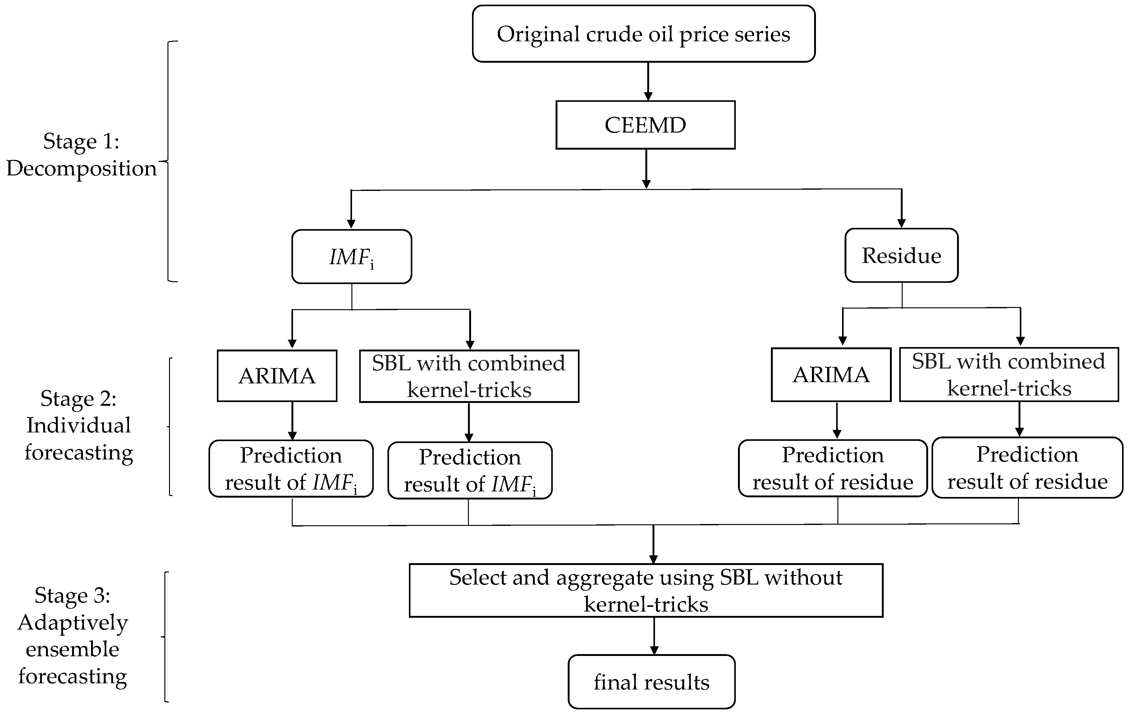
Inspired by the framework of “decomposition and ensemble”, this study proposes an adaptive hybrid ensemble model that integrates CEEMD, ARIMA and SBL with combined kernel-tricks, and SBL without kernel-tricks, termed as CEEMD-A&S-SBL, to forecast crude oil prices. The proposed model is shown in Figure 1, which includes three stages:
Stage 1: Decomposition. CEEMD is used to decompose the original series of crude oil prices into two parts: (1) K IMF components IMFj (j = 1, 2, …, K); (2) one residue component R.
Stage 2: Individual forecasting. The data samples in each decomposed component are respectively divided into a training set and a test set. The prediction models of ARIMA and SBL with combined kernel-tricks are built on the training set independently, and then, these two prediction models are applied to the test set separately.
Stage 3: Ensemble forecasting. These two groups of prediction results of all components are adaptively selected based on the training precision, and then are aggregated by SBL without kernel-tricks as the final forecasting results.
The proposed CEEMD-A&S-SBL employs the strategy of “divide and conquer”. The complex task of crude oil price forecasting is divided into a group of relatively simple sub-tasks of forecasting components independently. The CEEMD-A&S-SBL firstly applies CEEMD to decompose the original series of crude oil price into several components (IMFs and one residue), and each component contains some specific characteristics of crude oil prices. Generally, the first several IMFs imply high-frequency parts, while the last ones and the residue involve the low-frequency parts of crude oil prices. Secondly, the ARIMA and SBL with a combined kernel are independently applied to each component without distinguishing between high- and low-frequency in the prediction stage. We selected these two models because each belongs to one of the two typical types of differential prediction models (i.e., statistical method and AI method). ARIMA is one of the most representative statistical methods and SBL with a combined kernel, as a type of AI method, has been proven promising for crude oil price forecasting [6]. Finally, the predicted values of the above two models for each component are adaptively selected based on the training precision, and then are aggregated as the final forecasting results of crude oil prices using SBL without kernel-tricks. This framework of “decomposition and ensemble” makes it possible for the CEEMD-A&S-SBL to improve the performance of crude oil price forecasting.
Significantly, some recent studies applied differential models to forecast the high-frequency and low-frequency components separately. These studies obviously differed from the current research with respect to individual component forecasting and ensemble in that (1) they distinguished the decomposed crude oil prices into two parts: high-frequency and low-frequency components, and employed appropriate models to forecast the two parts; (2) they aggregated the prediction results of all components as the final forecasting results using simple addition or learning methods. In contrast, the current study uses two kinds of differential prediction models (i.e., ARIMA and SBL with combined kernel-tricks) to forecast each single component independently without identifying high-frequency and low-frequency, and then adaptively selects and aggregates the predicted values of two models as the final forecasting results of crude oil prices.
4. Experimental Results
4.1. Data Description
In order to better evaluate the performance of the proposed CEEMD-A&S-SBL, this study collected WTI and Brent crude oil spot prices in view of their representative significance in global crude oil markets. The daily closing price data set is divided into two subsets: the first 80% of sample data for training and the last 20% for testing. The training set is used to train models and optimize parameters, and the testing data set is applied to evaluate the performance of established prediction models. The divided samples of crude oil prices are shown in Table 1.
4.2. Evaluation Measures
In order to evaluate the model from multiple aspects, we employed four frequently used evaluation metrics, including two error indexes: the mean absolute percent error (MAPE) and the root mean squared error (RMSE), one direction index: the directional statistic (Dstat) and one statistic index: the Diebold–Mariano (DM) statistic. Firstly, MAPE and RMSE were selected to evaluate the prediction accuracy, as defined by Equations (14) and (15), respectively:
where is the predicted value and is the actual value at time t and n is the total number of data in a testing data set.
The Dstat was used to evaluate the ability of direction prediction, which is defined as follow:
where .
Generally, the smaller the MAPE and RMSE, the greater the Dstat, which represents a higher prediction accuracy and a better performance of direction prediction.
In order to better evaluate whether the prediction accuracy of the proposed prediction model is significantly better than those of previous models or not, the Diebold–Mariano (DM) statistic was introduced in this study, as defined by Equation (17):
where , and . are the predicted values of the first prediction model, and are those of the second prediction model at time t. When the DM statistic is negative, the first prediction model statistically outperforms the second one.
4.3. Experimental Settings
In this study, the development and evaluation of prediction model included three aspects:
First, previous research has demonstrated that ensemble models outperformed single models in crude oil price forecasting [6]. Therefore, the overall performance of CEEMD-A&S-SBL was only compared with that of some state-of-the-art ensemble prediction models in terms of the above evaluation metrics in this study. Thus, on the basis of the same crude oil price data, we evaluated whether our proposed CEEMD-A&S-SBL was effective for improving prediction precision. The compared models included one classical statistical method (ARIMA), three popular AI models (LSSVR, ANN, CK-SBL) and a hybrid model that forecasts high-frequency, low-frequency and trend components individually (HLT) [31]. In addition, since SBL with a combined kernel has shown better prediction performance compared with that with a single kernel, SBL with a combined kernel was selected as the predict model. Therefore, we had five individual prediction methods (ARIMA, LSSVR, ANN, CK-SBL and HLT) for each component to compare forecasting with A&S. All prediction methods are shown in Table 2.
Following the previous work [6], an adaptive PSO (APSO) method was used to optimize the parameters in CK-SBL, which adaptively adjusted the inertia weight of each particle based on the distance between the global best particle and the current one. In addition, the Akaike information criterion (AIC) [51] was used to determine the ARIMA parameters (p-d-q). RBF kernel was applied in LSSVR and grid search was used to seek the optimal parameters. For ANN, a back propagation neural network was employed, the number of hidden nodes was set to 10, and the iteration time was set to 10,000. For HLT, the PSO was used for adaptive parameter selection for LSSVR.
Second, we evaluated the three different decomposition methods (EMD, EEMD, CEEMD) for the proposed model in this study. In this phase, on the basis of same aggregation method (SBL) and prediction method (A&S), we evaluated the performance of different decomposition methods.
Third, we compared the two different ensemble methods (simple addition and SBL) for the proposed model in this study. In this phase, on the basis of same decomposition method (CEEMD) and prediction method (A&S), we evaluated the performance of the SBL ensemble method.
In addition, data normalization is an important work for computational efficiency and fair comparison of AI-based time series forecasting [6]. In this study, we applied the Min-Max normalization, a frequently-used normalization method, for AI-based predictors. It is worth pointing out that inverse normalization needs to be executed after the normalized predicted values are obtained. We conducted three-step-ahead predictions with horizon h = 1, 2, 3 and lag order lo = 6 in this study.
Especially, in CEEMD-A&S-SBL, the predicted values of the two differential models for each component were adaptively selected based on the training precision. Therefore, how to accurately evaluate the training precision is utmost important for adaptive selection of models. RMSE and MAPE are frequently used evaluation indexes. In this study, we selected RMSE mainly because there existed some actual zero values after CEEMD, thus RMSE was more effective for reflecting the training precision than MAPE.
All the experiments were performed by MATLAB R2017a on a 64-bit Microsoft Windows 10 with an i5-7820X CPU @1.8 GHz and 8 GB RAM.
4.4. Results and Analysis
4.4.1. Experimental Results of Overall Predictive Models
On the basis of same decomposition (i.e., CEEMD), we firstly compared the overall performance of the five extant prediction models (i.e., CEEMD-ARIMA-ADD, CEEMD-LSSVR-ADD, CEEMD-ANN-ADD, CEEMD-CK-SBL-ADD, CEEMD-HLT-ADD) with our proposed adaptively prediction model (CEEMD-A&S-SBL) in terms of MAPE, RMSE, and Dstat. We adopted these five models because they were the most frequently used and effective prediction methods [2,6,11,12,21,22,23,24,31]. Among all these models, ARIMA is one classical statistical method; LSSVR, ANN and CK-SBL are three popular AI models; HLT is one recent hybrid prediction model. The experimental results are reported in Table 3, Table 4 and Table 5, respectively.
Among all these models, CEEMD-A&S-SBL model achieved the lowest (the best) MAPE values in all cases on both markets. Although the previous hybrid model CEEMD-HLT-ADD achieved the lowest MAPE values compared with the single prediction models, the proposed hybrid model CEEMD-A&S-SBL outperformed the CEEMD-HLT-ADD model in all cases. For each prediction model, the MAPE values increased with the horizon.
Table 4 reported the RMSE values of all prediction models on WTI and Brent crude oil prices. It can be seen that CEEMD-A&S-SBL outperformed the hybrid model CEEMD-HLT-ADD and all single prediction models in all cases. Of all single models, the statistical model ARIMA obtained the worst RMSE values in all six cases. For the AI models, LSSVR, ANN and CK-SBL achieved close RMSE values, and the model CK-SBL was slightly better than others. As to the hybrid models, CEEMD-A&S-SBL achieved the lower RMSE values than CEEMD-HTL-ADD model, showing that the former was more powerful for crude oil price forecasting.
As to the directional statistics, it can be seen from Table 5 that CEEMD-A&S-SBL model achieved the highest values in five out of six cases, indicating that the CEEMD-A&S-SBL model had better performance in the direction forecasting of crude oil prices. For each model, the corresponding Dstat values decreased with the increase of the horizon. Amongst the single prediction models, ANN, LSSVR and CK-SBL obtained the higher Dstat values than ARIMA, showing that the AI models were capable of achieving better directional predictions compared with the statistical model ARIMA. Moreover, the hybrid models greatly outperformed the single prediction models.
From the overall results above, it can be seen that the hybrid prediction models consistently outperformed the single prediction models in all cases in terms of MAPE, RMSE, and Dstat. Between the two hybrid models, our proposed CEEMD-A&S-SBL achieved better prediction performance compared with CEEMD-HLT-ADD.
In order to better evaluate whether the prediction accuracy of CEEMD-A&S-SBL is significantly better than those of other models or not, the Diebold–Mariano (DM) test [52] was used in this study. The statistics and p-values (in brackets) are reported in Table 6 and Table 7.
DM test results on the prediction of WTI and Brent crude oil prices demonstrated that the CEEMD-A&S-SBL model significantly outperformed CEEMD-ARIMA-ADD, CEEMD-ANN-ADD, CEEMD-LSSVR-ADD, CEEMD-CK-SBL-ADD and CEEMD-HLT-ADD, and the corresponding p-values were much less than 0.05 in all cases.
On one hand, when we chose the single prediction models, including CEEMD-ARIMA-ADD, CEEMD-ANN-ADD, CEEMD-LSSVR-ADD, CEEMD-CK-SBL-ADD, as the benchmark models, CEEMD-A&S-SBL was statistically superior to these single prediction models, indicating that the former was more powerful for nonlinear and nonstationary crude oil price forecasting. On the other hand, when we chose the hybrid model CEEMD-HLT-ADD as the benchmark model, the prediction results of CEEMD-A&S-SBL were also significantly better. In summary, the hybrid model CEEMD-A&S-SBL achieved the best prediction accuracy in all models. The DM test results further statistically confirmed the conclusion.
4.4.2. Experimental Results of Decomposition Methods
On the basis of same prediction (A&S) and ensemble (SBL) methods, we evaluated the performance of the various decomposition methods. Table 8, Table 9 and Table 10 report the corresponding prediction results in terms of MAPE, RMSE and Dstat, respectively. It can be found that the CEEMD method was the best decomposition method that achieved the lowest MAPE and RMSE values and the highest Dstat values at each horizon.
In order to better evaluate whether the decomposition method CEEMD is significantly better than other decomposition methods or not, the DM test was used. The statistics and p-values (in brackets) are reported in Table 11. DM test results on the prediction of WTI and Brent crude oil prices demonstrated that the CEEMD decomposition method significantly outperformed EEMD and EMD in all cases, and the corresponding p-values were much less than 0.05 in all cases.
4.4.3. Experimental Results of Ensemble Methods
Traditional ensemble method uses addition operation. All IMFs and residue are simply added as the final forecasting results. In order to potentially enhance the prediction precision, SBL without kernel-tricks was chosen as the ensemble method in our proposed model. We chose SBL without kernel-tricks mainly because it is a kind of fast and efficient ensemble method. Table 12, Table 13 and Table 14 show the corresponding prediction results using addition or SBL ensemble method for A&S model in terms of MAPE, RMSE and Dstat, respectively. It can be easily seen that the SBL ensemble method outperformed the simple addition, achieving the lower MAPE and RMSE values, and the highest Dstat values at each horizon.
In order to better evaluate whether the SBL ensemble method is significantly better than the addition ensemble method, the DM test was used. The statistics and p-values (in brackets) are reported in Table 15. DM test results on the prediction of WTI and Brent crude oil prices showed that the SBL ensemble method significantly outperformed the simple addition method in all cases, and the corresponding p-values were much less than 0.05 in all cases.
4.5. Discussions
In order to better analyze the proposed CEEMD-A&S-SBL, we will further discuss some characteristics of the proposed model for forecasting crude oil prices, including CEEMD parameter settings, the impact of the lag order, individual component prediction model and selection and the weights of components in aggregation.
4.5.1. CEEMD Parameter Settings
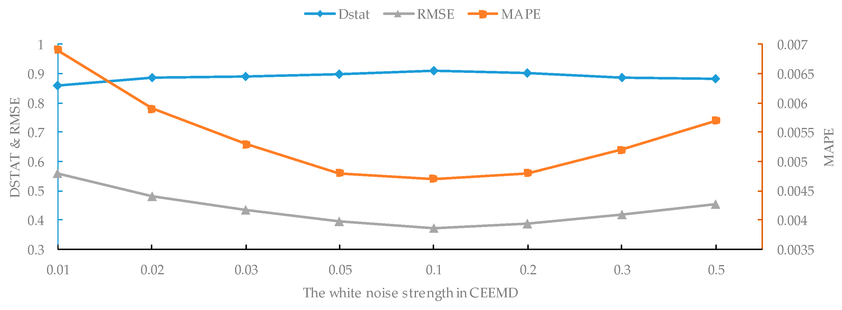
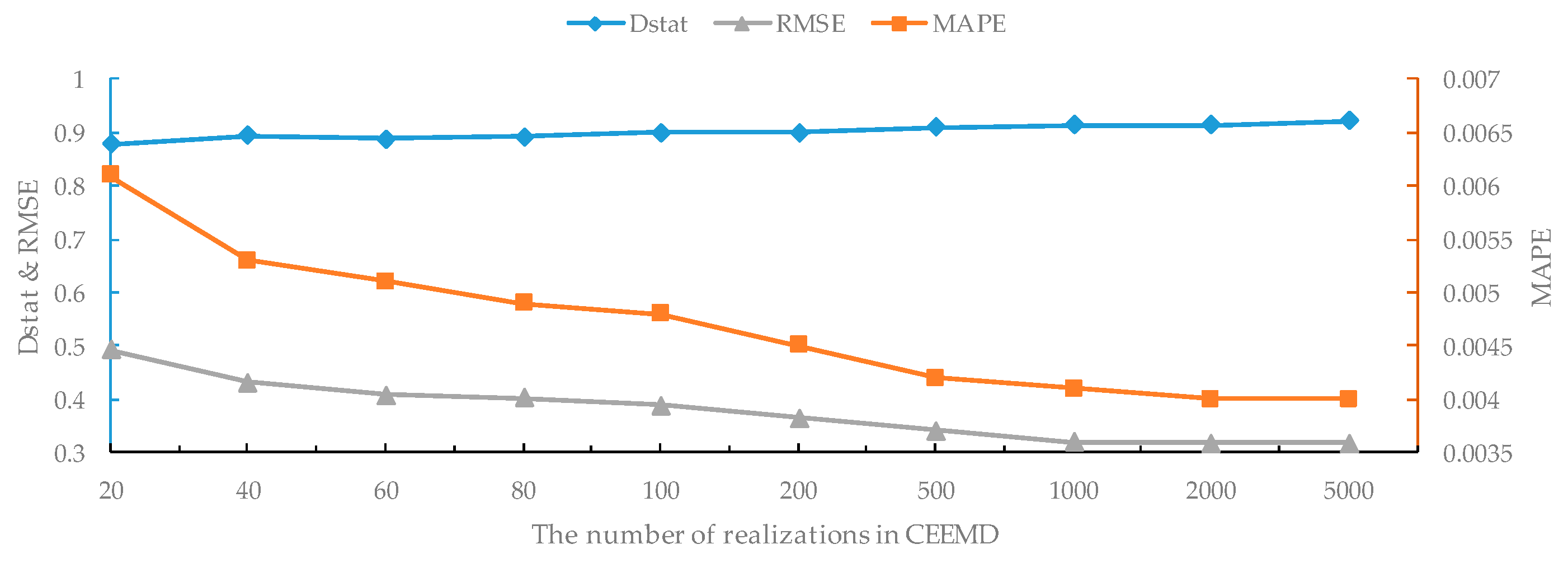
In the decomposition of the original series, a particular white noise was added at each stage of CEEMD. Let the parameter St be the white noise strength and I be the number of realizations in CEEMD. In order to investigate the impact of these parameters for crude oil price forecasting, we conducted the experiments on WTI crude oil prices with one-step-ahead forecasting. First, we fixed I = 100 and ran CEEMD-A&S-SBL with a variable St in the range of {0.01, 0.02, 0.03, 0.05, 0.1, 0.2, 0.3, 0.5}. The results are shown in Figure 4. Second, we fixed St = 0.2 and repeated the experiments with a variable I in the range of {20, 40, 60, 80, 100, 200, 500, 1000, 2000, 5000}; the results are shown in Figure 5.
As shown in Figure 4, the values of RMSE, MAPE and Dstat simultaneously achieve the best values when the noise strength in CEEMD equals to 0.1. When the noise strength is greater or less than 0.1, the prediction performance becomes worse and worse. This indicates that too much or too little added noise decreases the forecasting precision. The experimental results show that the noise strength has a significant impact on forecasting accuracy, and an ideal value of added noise strength is about 0.1.
On the other hand, with the increase of the number of realizations in CEEMD, the values of both RMSE and MAPE decrease and Dstat increases when the number of realizations is less than 1000, showing that the forecasting performance continuously improves as shown in Figure 5. However, when the number of realizations is greater than 1000, RMSE, MAPE and Dstat tend to be roughly stable. Therefore, if time cost is considered, 1000 is an appropriate value for the number of realizations in CEEMD in terms of RMSE, MAPE and Dstat.
4.5.2. The Impact of the Lag Order
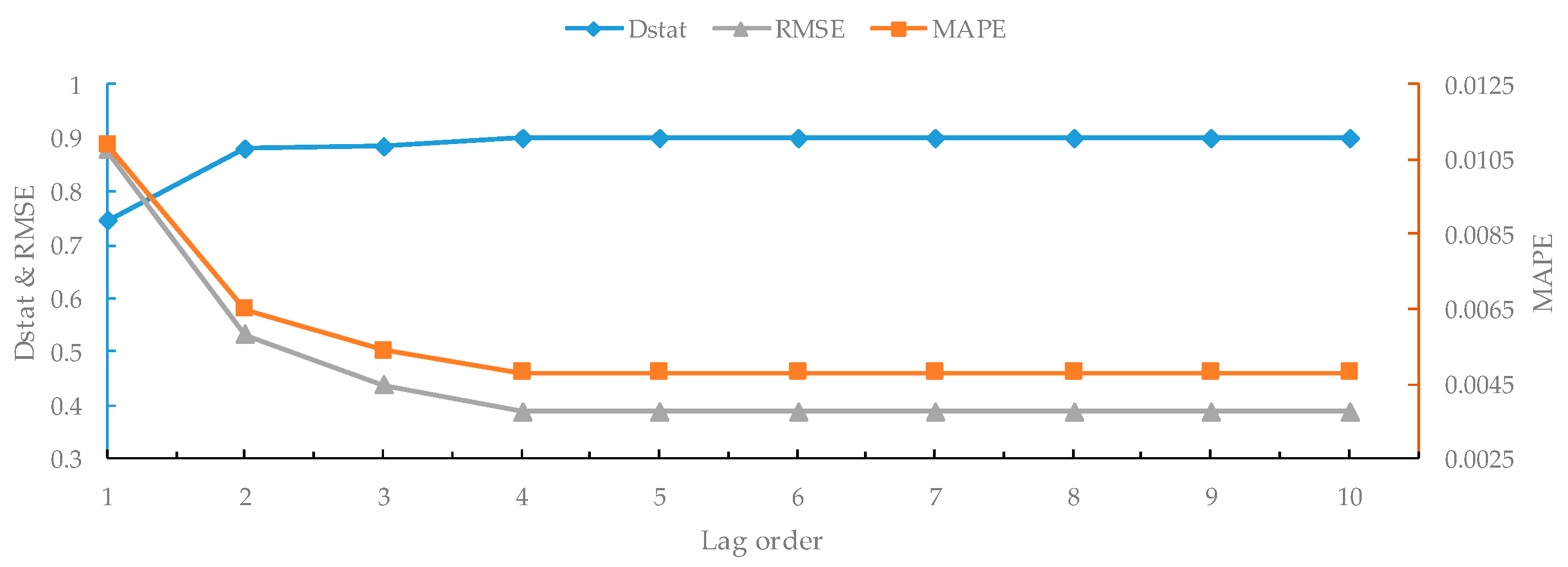
In order to further investigate the impact of the lag order on our proposed CEEMD-A&S-SBL model, we conducted the one-step-ahead forecasting experiment on WTI crude oil prices with the number of lag orders from 1 to 10. The results are shown in Figure 6. It can be seen that the forecasting performance significantly improves with the increase of the lag order from 1 to 4. Then, RMSE slightly decreases with the increase of lag order from 5 to 6, while MAPE and Dstat remain unchanged. When the lag order is greater than 6, all three metrics tend to be stable. The experimental results demonstrate that the lag order has a significant impact on forecasting accuracy, and an ideal value of lag order is about 6.
4.5.3. Individual Component Prediction Model and Selection
In the proposed CEEMD-A&S-SBL model, the prediction models of ARIMA and SBL with combined kernel-tricks are built on the training set independently for each component, and then these two prediction models are applied to the test set separately. These two groups of prediction results of all individual components are adaptively selected based on the training precision. Table 16 shows the prediction model selection results for each component in terms of RMSE.
From the above table, we can find that ARIMA and CK-SBL were adaptively selected for forecasting different components. For WTI crude oil data, CK-SBL was chosen for forecasting the IMF8, IMF9 and residue, while ARIMA was chosen for forecasting the rest of the components. Regarding Brent crude oil data, CK-SBL was chosen for forecasting the IMF6, IMF7 and IMF8, while ARIMA was chosen for forecasting the rest of the components. In the previous HTL model, the first IMFs were identified as low-frequency components and the rest as high-frequency ones, and then the appropriate models were employed to forecast the two parts respectively. Our proposed CEEMD-A&S-SBL model is capable to adaptively select appropriate prediction models based on the training precision without identifying the characteristic of each component. Therefore, the proposed CEEMD-A&S-SBL model is more flexible and can better adapt to differential components, showing higher forecasting performance on crude oil prices.
4.5.4. The Weights of Components in Aggregation
Most previous models aggregate the prediction results of all components as the final forecasting results using simple addition. The proposed CEEMD-A&S-SBL model uses SBL without kernel-tricks to aggregate the prediction values of individual components to obtain the final prediction results of crude oil prices. Table 17 shows the weights of components in aggregation using SBL for WTI and Brent oil price forecasting.
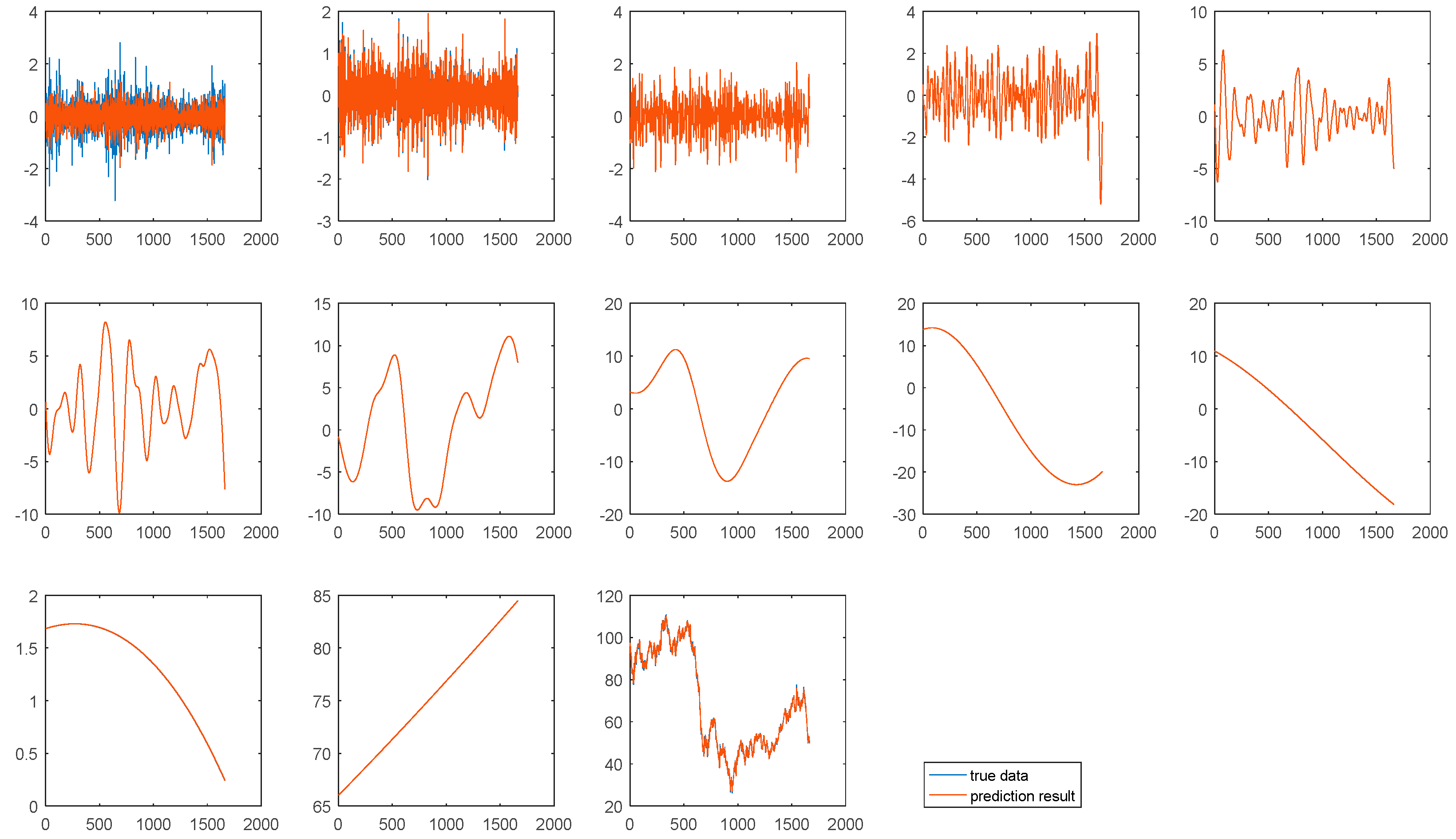
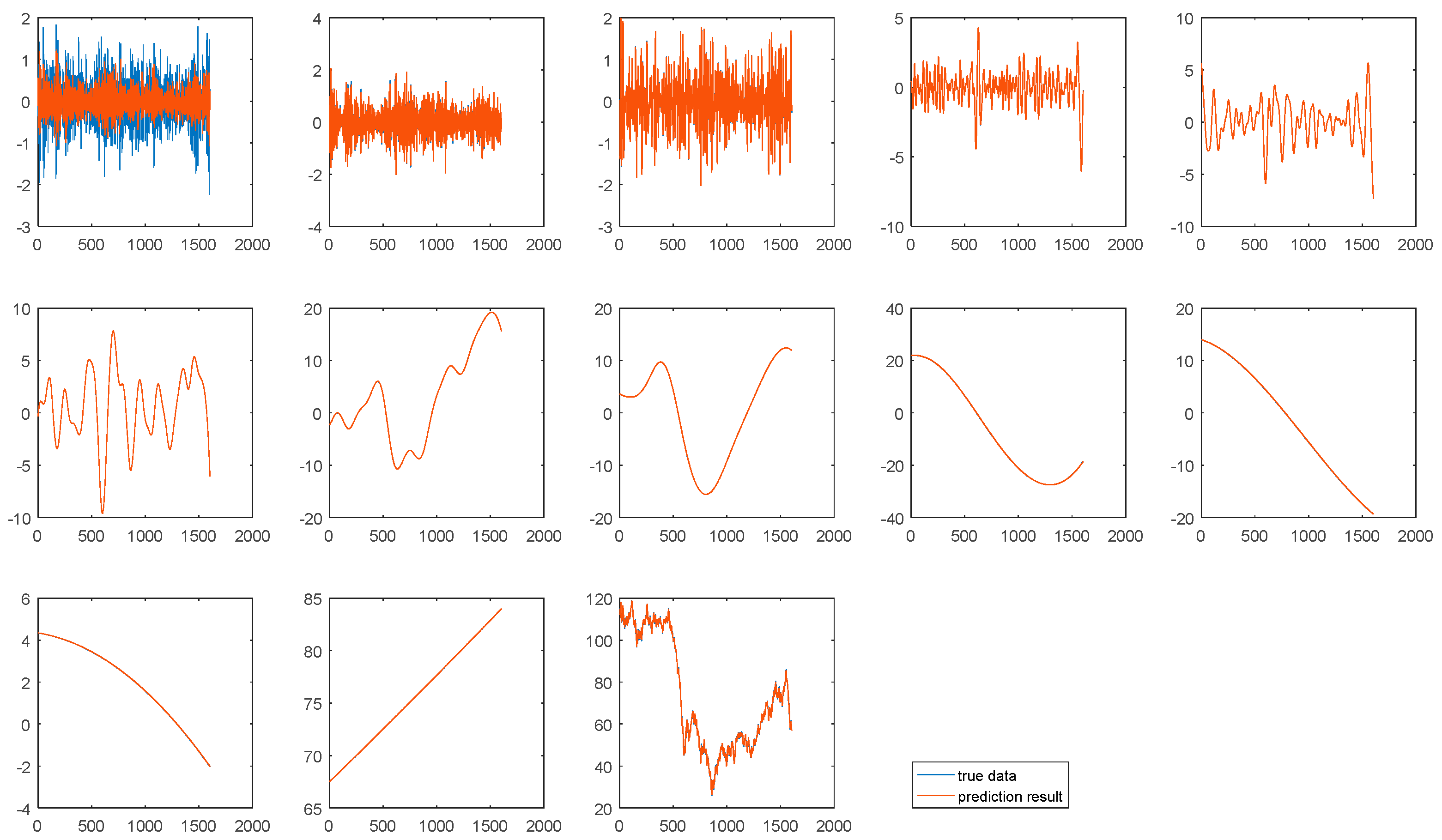
In the ensemble of addition, each component has an equal weight. It can be seen from Table 17 that each component has a differential aggregation weight when using the SBL ensemble. Especially, IMF1 has a relatively small weight mainly because IMF1 fluctuates dramatically, making it hard to accurately forecast. Figure 7 and Figure 8 show the prediction result of each component in one-step-ahead forecasting on WTI and Brent crude oil prices. It can be seen that all components can be accurately predicted except IMF1. Therefore, each component should have a differential weight in the aggregation stage. Due to the relatively larger prediction error, the IMF1 should have a relatively smaller weight in the aggregation stage. Compared with addition and other ensemble methods, ensemble using SBL has some advantages as follows: (1) good interpretability, (2) better prediction accuracy.
4.6. Summary
From the above results and analysis, some findings can be summarized as follows:
- (1)
- The AI models outperform the traditional statistical/econometric models in terms of MAPE, RMSE and Dstat, indicating that AI models are much better at forecasting nonlinear and nonstationary crude oil price series.
- (2)
- The hybrid ensemble models, including CEEMD-HLT-ADD and CEEMD-A&S-SBL, can further improve the prediction performance.
- (3)
- Our proposed prediction model CEEMD-A&S-SBL adaptively selects an appropriate prediction model for forecasting each component without identifying high-frequency and low-frequency in advance, and the adaptive hybrid model significantly outperforms the other compared hybrid model.
- (4)
- The CEEMD method achieves better prediction results than the counterpart EEMD and EMD methods, indicating that CEEMD is more suitable for decomposing original crude oil price series.
- (5)
- The SBL ensemble method outperforms the traditional addition method in terms of MAPE, RMSE and Dstat, showing that SBL is more suitable for aggregating individual prediction components.
5. Conclusions
It is a great challenge for the accurate forecast of crude oil prices because of its nonlinearity and nonstationarity. To better forecast the crude oil price time series, this paper proposed a novel adaptive hybrid ensemble learning paradigm (CEEMD-A&S-SBL) incorporating CEEMD, ARIMA and SBL. Firstly, the decomposition method CEEMD was employed to decompose the original time series of crude oil prices into several IMFs and one residue. In the individual forecasting phase, ARIMA and SBL with combined kernel-tricks were used to predict target values for the residue and each single IMF independently. Finally, the prediction results of the above two models for each component were adaptively selected based on the training precision, and then aggregated as the final forecasting results using SBL without kernel-tricks. To our knowledge, this is the first time that the adaptive model selection for individual component forecasting has been developed to forecast crude oil prices. The experimental results show that: (1) compared with five state-of-the-art prediction models, the proposed model can significantly improve the prediction accuracy of crude oil prices; (2) CEEMD is superior to EEMD and EMD for decomposing the original time series of crude oil prices; and (3) SBL outperforms addition method in aggregating the individual forecasting results of components.
Future work could be extended in four aspects: (1) selecting more appropriate prediction approaches to build the hybrid ensemble model for forecasting crude oil prices; (2) developing more metrics for evaluating the training precision instead of RMSE only; (3) applying the CEEMD-A&S-SBL to forecast other time series of energy, such as carbon price, wind speed and electricity load; and (4) assessing the scaling ability of CEEMD-A&S-SBL to other time series with various volume of data, such as hourly price series and weekly price series.
Author Contributions
Formal analysis, J.W.; Investigation, Y.C. and T.Z.; Methodology, J.W.; Software, J.W. and T.L.; Supervision, T.L.; Writing—Original draft, J.W.; Writing—Review & editing, J.W. and T.L.
Funding
This research was funded by the Fundamental Research Funds for the Central Universities, grant number JBK1902029, the Ministry of Education of Humanities and Social Science Project, grant number 19YJAZH047, and the Scientific Research Fund of Sichuan Provincial Education Department, grant number 17ZB0433.
Conflicts of Interest
The authors declare no conflict of interest.
References
- British Petroleum. BP Energy Outlook 2018. Available online: https://www.bp.com/en/global/corporate/energy-economics/energy-outlook.html (accessed on 29 January 2019).
- Li, T.; Hu, Z.; Jia, Y.; Wu, J.; Zhou, Y. Forecasting crude oil prices using ensemble empirical mode decomposition and sparse Bayesian learning. Energies 2018, 11, 1182. [Google Scholar] [CrossRef]
- Yu, L.; Wang, S.; Lai, K.K. Forecasting crude oil price with an EMD-based neural network ensemble learning paradigm. Energy Econ. 2008, 30, 2623–2635. [Google Scholar] [CrossRef]
- Yu, L.; Dai, W.; Tang, L.; Wu, J. A hybrid grid-GA-based LSSVR learning paradigm for crude oil price forecasting. Neural Comput. Appl. 2016, 27, 2193–2215. [Google Scholar] [CrossRef]
- He, K.; Yu, L.; Lai, K.K. Crude oil price analysis and forecasting using wavelet decomposed ensemble model. Energy 2012, 46, 564–574. [Google Scholar] [CrossRef]
- Li, T.; Zhou, M.; Guo, C.; Luo, M.; Wu, J.; Pan, F.; Tao, Q.; He, T. Forecasting crude oil price using EEMD and RVM with adaptive PSO-based kernels. Energies 2016, 9, 1014. [Google Scholar] [CrossRef]
- Baumeister, C.; Kilian, L. Real-time forecasts of the real price of oil. J. Bus. Econ. Stat. 2012, 30, 326–336. [Google Scholar] [CrossRef]
- Baumeister, C.; Kilian, L. What central bankers need to know about forecasting oil prices. Int. Econ. Rev. 2014, 55, 869–889. [Google Scholar] [CrossRef]
- Lanza, A.; Manera, M.; Giovannini, M. Modeling and forecasting cointegrated relationships among heavy oil and product prices. Energy Econ. 2005, 27, 831–848. [Google Scholar] [CrossRef]
- Murat, A.; Tokat, E. Forecasting oil price movements with crack spread futures. Energy Econ. 2009, 31, 85–90. [Google Scholar] [CrossRef]
- Koutroumanidis, T.; Ioannou, K.; Arabatzis, G. Predicting fuelwood prices in Greece with the use of ARIMA models, artificial neural networks and a hybrid ARIMA-ANN model. Energy Policy 2009, 37, 3627–3634. [Google Scholar] [CrossRef]
- Abledu, G.K.; Agbodah, K. Stochastic forecasting and modeling of volatility of oil prices in Ghana using ARIMA time series model. Eur. J. Bus. Manag. 2012, 4, 122–131. [Google Scholar]
- Morana, C. A semiparametric approach to short-term oil price forecasting. Energy Econ. 2001, 23, 325–338. [Google Scholar] [CrossRef]
- Hou, A.; Suardi, S. A nonparametric GARCH model of crude oil price return volatility. Energy Econ. 2012, 34, 618–626. [Google Scholar] [CrossRef]
- Mohammadi, H.; Su, L. International evidence on crude oil price dynamics: Applications of ARIMA-GARCH models. Energy Econ. 2010, 32, 1001–1008. [Google Scholar] [CrossRef]
- Wei, Y.; Wang, Y.; Huang, D. Forecasting crude oil market volatility: Further evidence using GARCH-class models. Energy Econ. 2010, 32, 1477–1484. [Google Scholar] [CrossRef]
- Kulkarni, S.; Haidar, I. Forecasting model for crude oil price using artificial neural networks and commodity futures prices. Int. J. Comput. Sci. Inf. Secur. 2009, 2, 81–88. [Google Scholar]
- Mirmirani, S.; Li, H.C. A comparison of VAR and Neural Networks with Genetic Algorithm in Forecasting Price of Oil. In Applications of Artificial Intelligence in Finance and Economics 2004; Emerald Group Publishing Limited: Bingley, UK, 2004; pp. 203–223. [Google Scholar]
- Haidar, I.; Kulkarni, S.; Pan, H. Forecasting Model for Crude Oil Prices Based on Artificial Neural Networks. In Proceedings of the Intelligent Sensors, Sensor Networks and Information Processing (ISSNIP 2008), Sydney, Australia, 15–18 December 2008; pp. 103–108. [Google Scholar]
- Mostafa, M.M.; El-Masry, A.A. Oil price forecasting using gene expression programming and artificial neural networks. Econ. Model. 2016, 54, 40–53. [Google Scholar] [CrossRef] [Green Version]
- Xie, W.; Yu, L.; Xu, S.; Wang, S. A new method for crude oil price forecasting based on support vector machines. In Computational Science—ICCS 2006; Springer: Berlin/Heidelberg, Germany, 2006; pp. 444–451. [Google Scholar]
- Li, S.; Ge, Y. Crude oil price prediction based on a dynamic correcting support vector regression machine. Abstr. Appl. Anal. 2013, 2013, 528678. [Google Scholar]
- Mustaffa, Z.; Yusof, Y.; Kamaruddin, S. Enhanced ABC-LSSVM for Energy fuel price prediction. J. Inf. Commun. Technol. 2013, 12, 73–101. [Google Scholar]
- Khashman, A.; Nwulu, N.I. Support Vector Machines Versus Back Propagation Algorithm for Oil Price Prediction. In Proceedings of the 8th International Symposium on Neural Networks (ISNN2011), Guilin, China, 29 May–1 June 2011; pp. 530–538. [Google Scholar]
- Wang, S.; Yu, L.; Lai, K.K. A Novel Hybrid AI System Framework for Crude Oil Price Forecasting. In Data Mining and Knowledge Management, Proceedings of the Chinese Academy of Sciences Symposium on Data Mining and Knowledge Management 2005, Beijing, China, 12–14 July 2004; Springer: Berlin/Heidelberg, Germany, 2005; pp. 233–242. [Google Scholar]
- Amin-Naseri, M.R.; Gharacheh, E.A. A Hybrid Artificial Intelligence Approach to Monthly Forecasting of Crude Oil Price Time Series. In Proceedings of the 10th International Conference on Engineering Applications of Neural Networks, Thessaloniki, Hellas, Greece, 29–31 August 2007; pp. 160–167. [Google Scholar]
- Tehrani, R.; Khodayar, F. A hybrid optimized artificial intelligent model to forecast crude oil using genetic algorithm. Afr. J. Bus. Manag. 2011, 5, 13130–13135. [Google Scholar] [CrossRef]
- Li, T.; Zhou, M. ECG classification using wavelet packet entropy and random forests. Entropy 2016, 18, 285. [Google Scholar] [CrossRef]
- Deng, W.; Zhang, S.; Zhao, H.; Yang, X. A novel fault diagnosis method based on integrating empirical wavelet transform and fuzzy entropy for motor bearing. IEEE Access 2018, 6, 35042–35056. [Google Scholar] [CrossRef]
- Zhao, H.; Meng, S.; Deng, W.; Yang, X. A new feature extraction method based on EEMD and multi-scale fuzzy entropy for motor bearing. Entropy 2017, 19, 14. [Google Scholar] [CrossRef]
- Zhu, B.; Shi, X.; Chevallier, J.; Wang, P.; Wei, Y.M. An adaptive multiscale ensemble learning paradigm for nonstationary and nonlinear energy price time series forecasting. J. Forecast. 2016, 35, 633–651. [Google Scholar] [CrossRef]
- Tang, L.; Dai, W.; Yu, L.; Wang, S. A novel CEEMD-based EELM ensemble learning paradigm for crude oil price forecasting. Int. J. Inf. Technol. Decis. Mak. 2015, 14, 141–169. [Google Scholar] [CrossRef]
- Huan, J.; Cao, W.; Qin, Y. Prediction of dissolved oxygen in aquaculture based on EEMD and LSSVM optimized by the Bayesian evidence framework. Comput. Electron. Agric. 2018, 150, 257–265. [Google Scholar] [CrossRef]
- Zhou, Y.; Li, T.; Shi, J.; Qian, Z. A CEEMDAN and XGBOOST-based approach to forecast crude oil prices. Complexity 2019, 2019. [Google Scholar] [CrossRef]
- Jammazi, R.; Aloui, C. Crude oil price forecasting: Experimental evidence from wavelet decomposition and neural network modeling. Energy Econ. 2012, 34, 828–841. [Google Scholar] [CrossRef]
- Zheng, H.; Yuan, J.; Chen, L. Short-term load forecasting using EMD-LSTM neural networks with a xgboost algorithm for feature importance evaluation. Energies 2017, 10, 1168. [Google Scholar] [CrossRef]
- Zhu, B.; Ye, S.; Wang, P.; He, K.; Zhang, T.; Wei, Y.M. A novel multiscale nonlinear ensemble leaning paradigm for carbon price forecasting. Energy Econ. 2018, 70, 143–157. [Google Scholar] [CrossRef]
- Fan, G.F.; Peng, L.L.; Hong, W.C.; Sun, F. Electric load forecasting by the SVR model with differential empirical mode decomposition and auto regression. Neurocomputing 2016, 173, 958–970. [Google Scholar] [CrossRef]
- Zhang, J.L.; Zhang, Y.J.; Zhang, L. A novel hybrid method for crude oil price forecasting. Energy Econ. 2015, 49, 649–659. [Google Scholar] [CrossRef]
- Torres, M.E.; Colominas, M.A.; Schlotthauer, G.; Flandrin, P. A Complete Ensemble Empirical Mode Decomposition with Adaptive Noise. In Proceedings of the IEEE International Conference on Acoustics, Speech and Signal Processing (ICASSP 2011), Prague, Czech Republic, 22–27 May 2011; pp. 4144–4147. [Google Scholar]
- Wu, Z.; Huang, N.E. Ensemble empirical mode decomposition: A noise-assisted data analysis method. Adv. Adapt. Data Anal. 2009, 1, 1–41. [Google Scholar] [CrossRef]
- Huang, N.E.; Shen, Z.; Long, S.R.; Wu, M.C.; Shih, H.H.; Zheng, Q.; Yen, N.C.; Tung, C.C.; Liu, H.H. The Empirical Mode Decomposition and the Hilbert Spectrum for Nonlinear and Non-Stationary Time Series Analysis. In Proceedings of the Royal Society of London A: Mathematical, Physical and Engineering Sciences 1998; The Royal Society: London, UK, 1998; pp. 903–995. [Google Scholar]
- Tipping, M.E. Sparse Bayesian learning and the relevance vector machine. J. Mach. Learn. Res. 2001, 1, 211–244. [Google Scholar]
- Ghosh, S.; Mujumdar, P.P. Statistical downscaling of GCM simulations to streamflow using relevance vector machine. Adv. Water Resour. 2008, 31, 132–146. [Google Scholar] [CrossRef]
- Li, T.; Zhang, Z. Robust face recognition via block sparse Bayesian learning. Math. Problems Eng. 2013, 2013. [Google Scholar] [CrossRef]
- Widodo, A.; Kim, E.Y.; Son, J.D.; Yang, B.S.; Tan, A.C.; Gu, D.S.; Choi, B.K.; Mathew, J. Fault diagnosis of low speed bearing based on relevance vector machine and support vector machine. Expert Syst. Appl. 2009, 36, 7252–7261. [Google Scholar] [CrossRef]
- Williams, O.; Blake, A.; Cipolla, R. Sparse bayesian learning for efficient visual tracking. IEEE Trans. Pattern Anal. Mach. Intell. 2005, 27, 1292–1304. [Google Scholar] [CrossRef]
- Zhang, Z.; Rao, B.D. Sparse signal recovery with temporally correlated source vectors using sparse Bayesian learning. IEEE J. Sel. Top. Signal Process. 2011, 5, 912–926. [Google Scholar] [CrossRef]
- Xu, X.M.; Mao, Y.F.; Xiong, J.N.; Zhou, F.L. Classification Performance Comparison between RVM and SVM. In Proceedings of the International Workshop on Anti-Counterfeiting, Security, Identification, Xiamen, China, 16–18 April 2007; pp. 208–211. [Google Scholar]
- Wipf, D.P.; Rao, B.D. Sparse Bayesian learning for basis selection. IEEE Trans. Signal Process. 2004, 52, 2153–2164. [Google Scholar] [CrossRef]
- Liu, H.; Tian, H.Q.; Li, Y.F. Comparison of two new ARIMA-ANN and ARIMA-Kalman hybrid methods for wind speed prediction. Appl. Energy 2012, 98, 415–424. [Google Scholar] [CrossRef]
- Diebold, F.X.; Mariano, R.S. Comparing predictive accuracy. J. Bus. Econ. Stat. 1995, 13, 253–263. [Google Scholar]
Figure 1.
The flowchart for the CEEMD-A&S-SBL. CEEMD: complete ensemble empirical mode decomposition; A&S: autoregressive integrated moving average (ARIMA) and sparse Bayesian learning (SBL); SBL: sparse Bayesian learning.
Figure 1.
The flowchart for the CEEMD-A&S-SBL. CEEMD: complete ensemble empirical mode decomposition; A&S: autoregressive integrated moving average (ARIMA) and sparse Bayesian learning (SBL); SBL: sparse Bayesian learning.

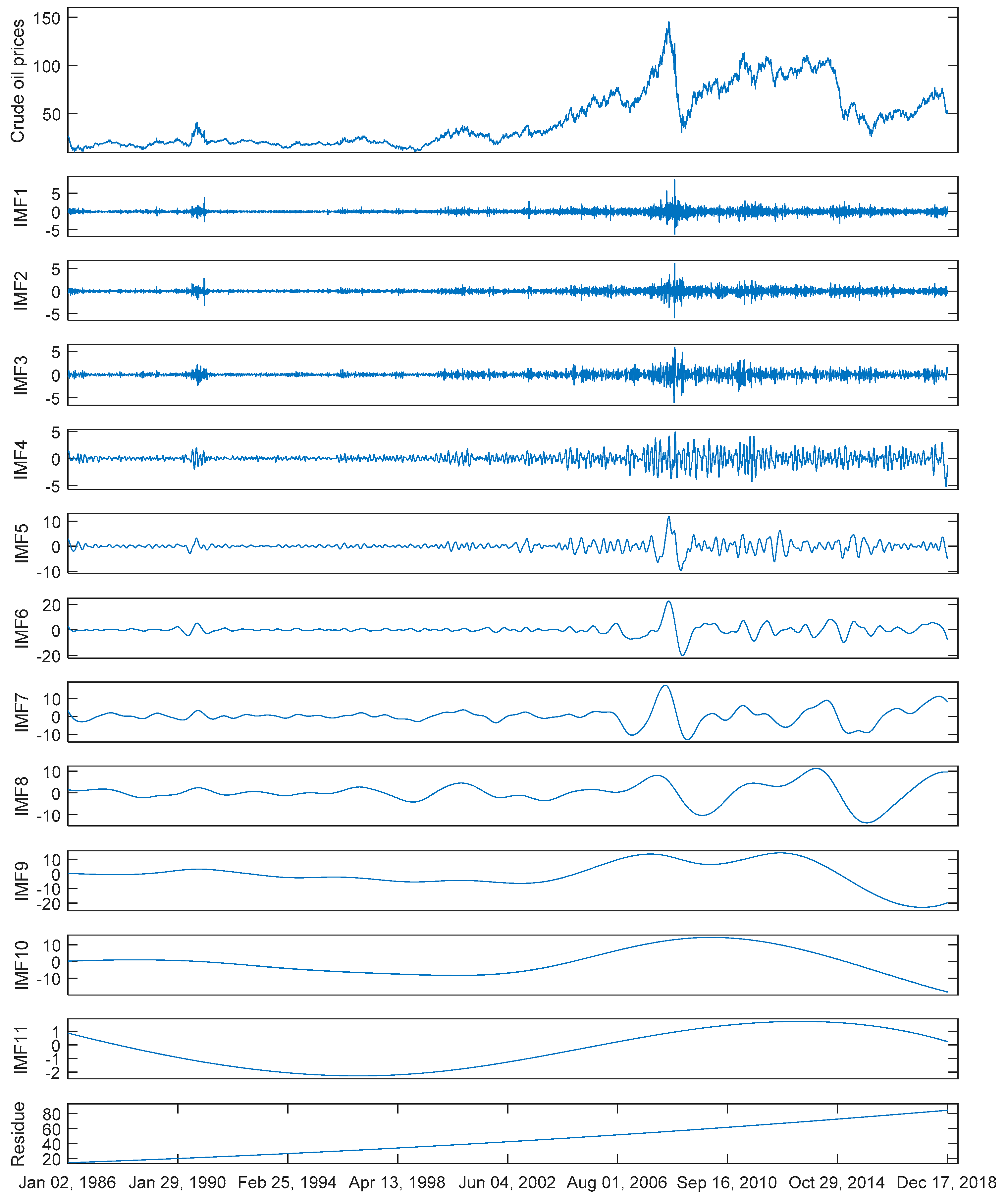
Figure 2.
The original series and corresponding components decomposed by complete ensemble empirical mode decomposition (CEEMD) of WTI crude oil prices.
Figure 2.
The original series and corresponding components decomposed by complete ensemble empirical mode decomposition (CEEMD) of WTI crude oil prices.

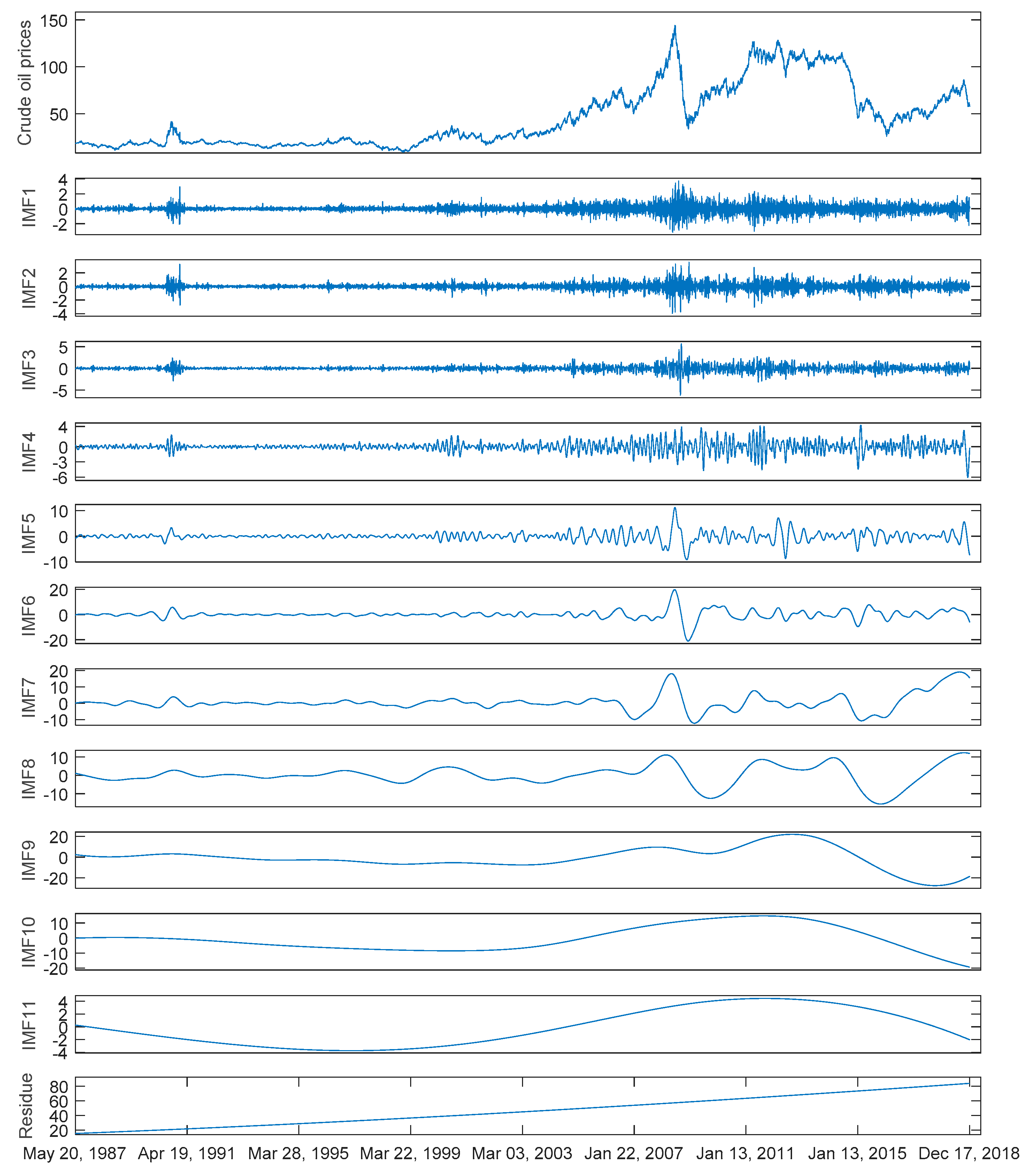
Figure 3.
The original series and corresponding components decomposed by CEEMD of Brent crude oil prices.
Figure 3.
The original series and corresponding components decomposed by CEEMD of Brent crude oil prices.

Figure 4.
The impact of the noise strength of CEEMD on WTI crude oil prices with one-step-ahead forecasting.
Figure 4.
The impact of the noise strength of CEEMD on WTI crude oil prices with one-step-ahead forecasting.

Figure 5.
The impact of the number of realizations of CEEMD on WTI crude oil prices with one-step-ahead forecasting.
Figure 5.
The impact of the number of realizations of CEEMD on WTI crude oil prices with one-step-ahead forecasting.

Figure 6.
The impact of lag order on WTI crude oil prices with one-step-ahead forecasting.

Figure 7.
Prediction result of each component in one-step-ahead forecasting on WTI crude oil prices.
Figure 7.
Prediction result of each component in one-step-ahead forecasting on WTI crude oil prices.

Figure 8.
Prediction result of each component in one-step-ahead forecasting on Brent crude oil prices.
Figure 8.
Prediction result of each component in one-step-ahead forecasting on Brent crude oil prices.


Table 1.
Samples of crude oil prices.
| Market | Size | Date | |
|---|---|---|---|
| West Texas Intermediate (WTI) | Sample set | 8312 | 2 January 1986~17 December 2018 |
| Training set | 6649 | 2 January 1986~9 May 2012 | |
| Testing set | 1663 | 10 May 2012~17 December 2018 | |
| Brent | Sample set | 8018 | 20 May 1987~17 December 2018 |
| Training set | 6414 | 20 May 1987~28 August 2012 | |
| Testing set | 1604 | 29 August 2012~17 December 2018 |
Table 2.
Descriptions of all the prediction methods in the experiments.
| Method | Description |
|---|---|
| ARIMA | Autoregressive integrated moving average |
| LSSVR | Least squares support vector regression |
| ANN | Back propagation neural network |
| CK-SBL | SBL with a combined kernel |
| HLT | ARIMA for high-frequency components and combined kernel LSSVR for low-frequency and trend components |
| A&S | All component are predicted by ARIMA and CK-SBL independently and then are aggregated adaptively |
Table 3.
The mean absolute percent error (MAPE) values of different prediction models on WTI and Brent crude oil prices.
Table 3.
The mean absolute percent error (MAPE) values of different prediction models on WTI and Brent crude oil prices.
| Market | Horizon | CEEMD-ARIMA-ADD | CEEMD-LSSVR-ADD | CEEMD-ANN-ADD | CEEMD-CK-SBL-ADD | CEEMD-HLT-ADD | CEEMD-A&S-SBL |
|---|---|---|---|---|---|---|---|
| WTI | One | 0.0169 | 0.0063 | 0.0120 | 0.0058 | 0.0049 | 0.0048 |
| Two | 0.0302 | 0.0080 | 0.0184 | 0.0079 | 0.0075 | 0.0074 | |
| Three | 0.0371 | 0.0111 | 0.0279 | 0.0099 | 0.0082 | 0.0081 | |
| Brent | One | 0.0408 | 0.0057 | 0.0146 | 0.0053 | 0.0044 | 0.0043 |
| Two | 0.0824 | 0.0080 | 0.0423 | 0.0071 | 0.0066 | 0.0065 | |
| Three | 0.1158 | 0.0106 | 0.0254 | 0.0092 | 0.0075 | 0.0074 |
CEEMD: complete ensemble empirical mode decomposition; ARIMA: autoregressive integrated moving average; LSSVR: least squares support vector regression; ANN: back propagation neural network; SBL: sparse Bayesian learning; CK-SBL: SBL with a combined kernel; HLT: a hybrid model that forecasts high-frequency, low-frequency and trend components individually; ADD: addition.
Table 4.
The root mean squared error (RMSE) values of different prediction models on WTI and Brent crude oil prices.
Table 4.
The root mean squared error (RMSE) values of different prediction models on WTI and Brent crude oil prices.
| Market | Horizon | CEEMD-ARIMA-ADD | CEEMD-LSSVR-ADD | CEEMD-ANN-ADD | CEEMD-CK-SBL-ADD | CEEMD-HLT-ADD | CEEMD-A&S-SBL |
|---|---|---|---|---|---|---|---|
| WTI | One | 1.0983 | 0.5317 | 0.9536 | 0.4766 | 0.3963 | 0.3878 |
| Two | 1.9390 | 0.6468 | 1.3625 | 0.6425 | 0.6113 | 0.5977 | |
| Three | 2.3850 | 0.9331 | 2.2405 | 0.7883 | 0.6578 | 0.6474 | |
| Brent | One | 3.0815 | 0.4494 | 1.1034 | 0.4410 | 0.3697 | 0.3590 |
| Two | 6.2689 | 0.6611 | 3.6149 | 0.5902 | 0.5560 | 0.5424 | |
| Three | 8.8840 | 0.8237 | 2.0899 | 0.7536 | 0.6251 | 0.6111 |
Table 5.
The directional statistic (Dstat) values of different prediction models on WTI and Brent crude oil prices.
Table 5.
The directional statistic (Dstat) values of different prediction models on WTI and Brent crude oil prices.
| Market | Horizon | CEEMD-ARIMA-ADD | CEEMD-LSSVR-ADD | CEEMD-ANN-ADD | CEEMD-CK-SBL-ADD | CEEMD-HLT-ADD | CEEMD-A&S-SBL |
|---|---|---|---|---|---|---|---|
| WTI | One | 0.6949 | 0.8598 | 0.8147 | 0.8712 | 0.8995 | 0.9007 |
| Two | 0.5716 | 0.8303 | 0.7244 | 0.8388 | 0.8394 | 0.8418 | |
| Three | 0.5626 | 0.7521 | 0.7118 | 0.7593 | 0.8135 | 0.8147 | |
| Brent | One | 0.6301 | 0.8528 | 0.7511 | 0.8740 | 0.8734 | 0.8784 |
| Two | 0.5727 | 0.7972 | 0.6925 | 0.8447 | 0.8390 | 0.8422 | |
| Three | 0.5527 | 0.7480 | 0.6881 | 0.7698 | 0.8091 | 0.8185 |
Table 6.
The Diebold–Mariano (DM) test results on WTI crude oil prices.
| Horizon | Tested Model | Benchmark Model | ||||
|---|---|---|---|---|---|---|
| CEEMD-ARIMA-ADD | CEEMD-ANN-ADD | CEEMD-LSSVR-ADD | CEEMD-CK-SBL-ADD | CEEMD-HLT-ADD | ||
| One | CEEMD-ANN-ADD | −6.401 (0.000) | ||||
| CEEMD-LSSVR-ADD | −37.579 (0.000) | −22.376 (0.000) | ||||
| CEEMD-CK-SBL-ADD | −34.935 (0.000) | −20.175 (0.000) | −4.014 (0.000) | |||
| CEEMD-HLT-ADD | −39.696 (0.000) | −23.213 (0.000) | −10.167 (0.000) | −9.846 (0.000) | ||
| CEEMD-A&S-SBL | −39.822 (0.000) | −23.262 (0.000) | −10.865 (0.000) | −9.971 (0.000) | −3.682 (0.000) | |
| Two | CEEMD-ANN-ADD | −17.100 (0.000) | ||||
| CEEMD-LSSVR-ADD | −41.834 (0.000) | −21.798 (0.000) | ||||
| CEEMD-CK-SBL-ADD | −41.245 (0.000) | −22.272 (0.000) | −0.406 (0.685) | |||
| CEEMD-HLT-ADD | −42.080 (0.000) | −23.126 (0.000) | −4.288 (0.000) | −4.984 (0.000) | ||
| CEEMD-A&S-SBL | −42.329 (0.000) | −23.339 (0.000) | −5.489 (0.000) | −5.710 (0.000) | −3.887 (0.000) | |
| Three | CEEMD-ANN-ADD | −2.722 (0.007) | ||||
| CEEMD-LSSVR-ADD | −43.031 (0.000) | −24.609 (0.000) | ||||
| CEEMD-CK-SBL-ADD | −41.550 (0.000) | −24.130 (0.000) | −6.002 (0.000) | |||
| CEEMD-HLT-ADD | −43.561 (0.000) | −25.395 (0.000) | −11.064 (0.000) | −12.549 (0.000) | ||
| CEEMD-A&S-SBL | −43.684 (0.000) | −25.423 (0.000) | −1.290 (0.000) | −11.200 (0.000) | −2.792 (0.005) | |
Table 7.
The Diebold–Mariano (DM) test results on Brent crude oil prices.
| Horizon | Tested Model | Benchmark Model | ||||
|---|---|---|---|---|---|---|
| CEEMD-ARIMA-ADD | CEEMD-ANN-ADD | CEEMD-LSSVR-ADD | CEEMD-CK-SBL-ADD | CEEMD-HLT-ADD | ||
| One | CEEMD-ANN-ADD | −24.977 (0.000) | ||||
| CEEMD-LSSVR-ADD | −25.324 (0.000) | −19.530 (0.000) | ||||
| CEEMD-CK-SBL-ADD | −25.333 (0.000) | −19.737 (0.000) | −0.934 (0.350) | |||
| CEEMD-HLT-ADD | −25.500 (0.000) | −21.137 (0.000) | −9.783 (0.000) | −9.724 (0.000) | ||
| CEEMD-A&S-SBL | −25.521 (0.000) | −21.339 (0.000) | −10.420 (0.000) | −10.095 (0.000) | −4.202(0.000) | |
| Two | CEEMD-ANN-ADD | −16.241 (0.000) | ||||
| CEEMD-LSSVR-ADD | −25.250 (0.000) | −26.451 (0.000) | ||||
| CEEMD-CK-SBL-ADD | −25.273 (0.000) | −26.728 (0.000) | −6.775 (0.000) | |||
| CEEMD-HLT-ADD | −25.299 (0.000) | −26.814 (0.000) | −10.215 (0.000) | −6.072 (0.000) | ||
| CEEMD-A&S-SBL | −25.311 (0.000) | −26.847 (0.000) | −10.869 (0.000) | −6.949 (0.000) | −4.261(0.000) | |
| Three | CEEMD-ANN-ADD | −23.494 (0.000) | ||||
| CEEMD-LSSVR-ADD | −24.832 (0.000) | −22.274 (0.000) | ||||
| CEEMD-CK-SBL-ADD | −24.841 (0.000) | −23.071 (0.000) | −4.521 (0.000) | |||
| CEEMD-HLT-ADD | −24.898 (0.000) | −24.284 (0.000) | −13.058 (0.000) | −12.715 (0.000) | ||
| CEEMD-A&S-SBL | −24.9040 (0.000) | −24.394 (0.000) | −12.995 (0.000) | −11.982 (0.000) | −4.135(0.000) | |
Table 8.
The MAPE values of different decomposition methods on WTI and Brent crude oil prices.
| Market | Horizon | EMD | EEMD | CEEMD |
|---|---|---|---|---|
| WTI | One | 0.0083 | 0.0079 | 0.0048 |
| Two | 0.0100 | 0.0095 | 0.0074 | |
| Three | 0.0117 | 0.0097 | 0.0081 | |
| Brent | One | 0.0078 | 0.0079 | 0.0043 |
| Two | 0.0091 | 0.0089 | 0.0065 | |
| Three | 0.0112 | 0.0091 | 0.0074 |
Table 9.
The RMSE values of different decomposition methods on WTI and Brent crude oil prices.
| Market | Horizon | EMD | EEMD | CEEMD |
|---|---|---|---|---|
| WTI | One | 0.6661 | 0.6225 | 0.3878 |
| Two | 0.8185 | 0.7511 | 0.5977 | |
| Three | 0.9497 | 0.7758 | 0.6474 | |
| Brent | One | 0.6750 | 0.6447 | 0.3590 |
| Two | 0.7713 | 0.7274 | 0.5424 | |
| Three | 0.9296 | 0.7456 | 0.6111 |
Table 10.
The Dstat values of decomposition methods on WTI and Brent crude oil prices.
| Market | Horizon | EMD | EEMD | CEEMD |
|---|---|---|---|---|
| WTI | One | 0.8189 | 0.8189 | 0.9007 |
| Two | 0.7966 | 0.7768 | 0.8418 | |
| Three | 0.7341 | 0.7714 | 0.8147 | |
| Brent | One | 0.8341 | 0.7998 | 0.8784 |
| Two | 0.8035 | 0.7711 | 0.8422 | |
| Three | 0.7299 | 0.7623 | 0.8185 |
Table 11.
The Diebold–Mariano (DM) test results on WTI and Brent crude oil prices.
| Market | Horizon | Tested Model | Benchmark Model | |
|---|---|---|---|---|
| EMD | EEMD | |||
| WTI | One | EEMD | −2.373 (0.018) | |
| CEEMD | −14.79 (0.000) | −15.93 (0.000) | ||
| Two | EEMD | −3.168 (0.002) | ||
| CEEMD | −11.63 (0.000) | −11.12 (0.000) | ||
| Three | EEMD | −8.208 (0.000) | ||
| CEEMD | −14.04 (0.000) | −9.944 (0.000) | ||
| Brent | One | EEMD | −1.143 (0.253) | |
| CEEMD | −9.993 (0.000) | −18.632 (0.000) | ||
| Two | EEMD | −2.172 (0.030) | ||
| CEEMD | −11.296 (0.000) | −13.513 (0.000) | ||
| Three | EEMD | −9.024 (0.000) | ||
| CEEMD | −14.566 (0.000) | −10.694 (0.000) | ||
Table 12.
The MAPE values of different prediction models on WTI and Brent crude oil prices.
| Market | Horizon | CEEMD-A&S-ADD | CEEMD-A&S-SBL |
|---|---|---|---|
| WTI | One | 0.0049 | 0.0048 |
| Two | 0.0075 | 0.0074 | |
| Three | 0.0082 | 0.0081 | |
| Brent | One | 0.0044 | 0.0043 |
| Two | 0.0066 | 0.0065 | |
| Three | 0.0075 | 0.0074 |
Table 13.
The RMSE values of different prediction models on WTI and Brent crude oil prices.
| Market | Horizon | CEEMD-A&S-ADD | CEEMD-A&S-SBL |
|---|---|---|---|
| WTI | One | 0.3955 | 0.3878 |
| Two | 0.6106 | 0.5977 | |
| Three | 0.6562 | 0.6474 | |
| Brent | One | 0.3659 | 0.3590 |
| Two | 0.5555 | 0.5424 | |
| Three | 0.6247 | 0.6111 |
Table 14.
The Dstat values of different prediction models on WTI and Brent crude oil prices.
| Market | Horizon | CEEMD-A&S-ADD | CEEMD-A&S-SBL |
|---|---|---|---|
| WTI | One | 0.9001 | 0.9007 |
| Two | 0.8388 | 0.8418 | |
| Three | 0.8123 | 0.8147 | |
| Brent | One | 0.8727 | 0.8784 |
| Two | 0.8421 | 0.8422 | |
| Three | 0.8110 | 0.8185 |
Table 15.
The Diebold–Mariano (DM) test results on WTI and Brent crude oil prices.
| Market | Horizon | Tested Model | Benchmark Model |
|---|---|---|---|
| Addition | |||
| WTI | One | SBL | −3.402 (0.001) |
| Two | SBL | −3.764 (0.000) | |
| Three | SBL | −2.333 (0.020) | |
| Brent | One | SBL | −2.952 (0.003) |
| Two | SBL | −4.336 (0.000) | |
| Three | SBL | −4.146 (0.000) |
Table 16.
Prediction model selection for each component on WTI and Brent crude oil prices.
| Market | IMF1 | IMF2 | IMF3 | IMF4 | IMF5 | IMF6 | IMF7 | IMF8 | IMF9 | IMF10 | IMF11 | Residue |
|---|---|---|---|---|---|---|---|---|---|---|---|---|
| WTI | ARIMA | ARIMA | ARIMA | ARIMA | ARIMA | ARIMA | ARIMA | CK-SBL | CK-SBL | ARIMA | ARIMA | CK-SBL |
| Brent | ARIMA | ARIMA | ARIMA | ARIMA | ARIMA | CK-SBL | CK-SBL | CK-SBL | ARIMA | ARIMA | ARIMA | ARIMA |
Table 17.
Weights of components in aggregation using SBL.
| Market | IMF1 | IMF2 | IMF3 | IMF4 | IMF5 | IMF6 | IMF7 | IMF8 | IMF9 | IMF10 | IMF11 | Residue |
|---|---|---|---|---|---|---|---|---|---|---|---|---|
| WTI | 0.9296 | 1.1345 | 0.9983 | 1.0038 | 0.9925 | 1.0032 | 0.9969 | 0.9982 | 1.0050 | 0.9938 | 1.0140 | 1.0001 |
| Brent | 0.9256 | 1.1440 | 1.0241 | 1.0146 | 1.0004 | 1.0013 | 0.9988 | 1.0001 | 1.0009 | 0.9979 | 1.0035 | 1.0000 |
© 2019 by the authors. Licensee MDPI, Basel, Switzerland. This article is an open access article distributed under the terms and conditions of the Creative Commons Attribution (CC BY) license (http://creativecommons.org/licenses/by/4.0/).
Share and Cite
MDPI and ACS Style
Wu, J.; Chen, Y.; Zhou, T.; Li, T. An Adaptive Hybrid Learning Paradigm Integrating CEEMD, ARIMA and SBL for Crude Oil Price Forecasting. Energies 2019, 12, 1239. https://doi.org/10.3390/en12071239
AMA Style
Wu J, Chen Y, Zhou T, Li T. An Adaptive Hybrid Learning Paradigm Integrating CEEMD, ARIMA and SBL for Crude Oil Price Forecasting. Energies. 2019; 12(7):1239. https://doi.org/10.3390/en12071239
Chicago/Turabian StyleWu, Jiang, Yu Chen, Tengfei Zhou, and Taiyong Li. 2019. "An Adaptive Hybrid Learning Paradigm Integrating CEEMD, ARIMA and SBL for Crude Oil Price Forecasting" Energies 12, no. 7: 1239. https://doi.org/10.3390/en12071239
Note that from the first issue of 2016, this journal uses article numbers instead of page numbers. See further details here.