1. Introduction
Methods to produce sharper delineated objects at depth using ground penetrating radar (GPR) is a continuing topic of study. Imaging results from ground-based scans and scans at various heights have benefited from the Gaussian mixture model (GMM) feature of the expectation-maximization (EM) algorithm technique [
1,
2,
3,
4,
5] of combining scans at differing frequencies over the same terrain. It is well known that GPR scans at high frequencies better illuminate objects close to the surface with great fidelity and lower frequencies delineate objects at lower depths with less detail. We reported that combining scans at several frequencies “smartly” increased the resolution of objects at lower depths [
1,
2,
3,
4,
5]. Scans were combined by using the GMM feature of the EM algorithm to sum weighted versions of each scan rather than just summing them together. We reported similar progress with GPR scans at various heights above ground [
5]. There are areas that remain to be explored, such as better edge detection for buried objects and the use of other excitation functions with similar characteristics to the Ricker pulse used most often in GPR systems.
In this paper, we explore using a chirp excitation function-based radar to replace the multiple frequency scans used in the EM GMM algorithm analysis, comparing the result with EM processed scans. In
Section 2, we discuss related work to combining GPR scans and processing scans with alternative excitation functions. In
Section 3, we describe the EM data mixture process [
6,
7], briefly covering the maximum likelihood (ML) estimation process as it relates to the EM algorithm. In
Section 4, we describe the chirp excitation function-based radar signal proposed for this analysis. In
Section 5, we present results of the comparison of compositing simulated GPR scans at various frequencies with the result using a chirp excitation function-based radar signal, all computed using the GprMax [
8] software program to develop the scan results. In
Section 6, we draw conclusions and discuss future work.
2. Related Work
In the literature, chirp waveforms are mentioned in reference to synthetic aperture radar (SAR) [
9,
10,
11] pulses and to a ground-based method called the vibroseis (seismic vibrator) technique [
12,
13,
14,
15]. chirp waveforms are used in SAR systems to reduce the amount of power needed by the transmitter. Included among the benefits of using chirp waveforms is the size of the transmitter can be reduced allowing for smaller airborne radar systems. Implementing pulse compression techniques improves the signal to noise ratio. This, in conjunction with signal compression (correlation of received and transmitted signal), increases the range resolution and enhances object detection capability. Stolt [
16], Gazdag [
17], or FK(ω-k) migration [
18,
19] techniques were used to account for phase shifts due to the angles radar signals were sent and received from; they are not always the same.
Vibroseis [
12,
13,
14,
15] is a ground-based method consisting of low frequency vibrations generated by using a shaker or piston driven mass, creating a low-frequency chirp signal, often used for oil exploration. The vibroseis [
12,
13,
14,
15] method was developed and trademarked by Continental Oil Company (Conoco). chirp signals from SAR and seismic vibration devices are processed in the same manner: cross-correlation of the reflections with the source signal determining wavelets representing target reflections. The use of a chirp waveform is our attempt to generate a response similar to the multiple frequency GPR scans combined by EM processing.
Our EM developed method, the compositing of GPR scans [
1,
2,
3,
4,
5], was preceded by Dougherty et al. [
20] who focused on a method to subtract the direct arrival pulse and combine each signal weighted with equal magnitudes. Booth et al. [
21,
22] followed Dougherty et al. [
20] repeating their method but adding a frequency scan weighting technique using trace averaged amplitude spectra. Time invariant weighting methods were proposed by Booth et al. [
21,
22] matching compositing results to a least-squares idealized amplitude spectrum. Bancroft [
23] introduced a method computing weights using one ramp to suppress a frequency’s energy while using another ramp to increase a frequency’s energy over time. Ramp start and stop times were determined by the wavelength of the frequency of interest. Bancroft also introduced weights based on the ratio of the average envelope of GPR frequencies used in the scans. Both methods, Booth et al. and Bancroft, provided minimal improvement over previous works. Our EM GMM method presented the best results of methods mentioned. The outcomes of these comparisons are detailed in references [
3,
4].
3. Expectation-Maximization Data Mixture Process
The EM algorithm is used to solve incomplete data problems [
6,
7], to determine membership weights of a collection of data points in a cluster, or to group like items in complex mixtures. Our expectation-maximization data mixture process exploits these features by defining a collection of data points in a cluster as a Gaussian mixture model (GMM) with membership weights. Then, using maximum likelihood (ML) parameter estimation to make the initial estimates of the unknown membership weights, establishing an ML estimation problem to solve. The EM algorithm reduces the ML estimation problem to a simpler optimization sub-problem which is guaranteed to converge.
We used the Gaussian mathematical distribution for the mixture model because it is often used when the distribution of the data is unknown. We define a finite mixture model as
f(x;θ), of
K mixture components of the following GMM function:
where:
The EM algorithm is an iterative process with two steps. The expectation step is the first step (E-step). The conditional expectation of the group of membership weights, for , are determined during this step. Unobservable data based on the mean and covariance matrix, , is integrated into the model. The maximization step (M-step) is the second step. In this step, new parameter values to maximize the finite mixture model are calculated: mixture weights, the mean, and covariance of the weights . The E-step and M-step are repeated until the GMM model converges, defined by a minimal change of the log-likelihood of the GMM function from one iteration to the next. The E-step and M-step are defined below:
MATLAB programming language was used to implement these equations (MATLAB—a proprietary numerical programming language developed by The MathWorks, Inc. of Natick, MA., USA). In the GMM model, the variable ‘k’ represents the different scanning frequencies, and ‘x’ represents the GPR trace scans. Each GPR trace at a frequency transmitter (Tx), and receiver (Rx) position is analyzed and combined for all frequencies before moving on to the next position. The EM GMM processing steps are as follows.
EM GMM process:
Initialize algorithm parameters—weights (mixture and group membership), mean, covariance, for each trace.
E-Step—estimate parameters.
M-Step—maximize estimated parameters.
Check for convergence—log-likelihood of mixture model.
Repeat steps 2–4 until change from iteration to iteration is below or equal to a predefined value.
Combine traces with defined mixture weights.
The ML estimation process provides an estimate of an unknown parameter by determining the value that maximizes the probability of realizing the data we observed (likelihood). This process becomes hard when there are at least two sets of data and one is partially observed or hidden and the mixture parameters are to be estimated. For the case where there is only one unknown parameter, the ML estimation process can be described as follows. Given a random sample X
1, X
2, …, X
n, independent and identically distributed (i.i.d.), with a probability density function (PDF) of
with an unknown parameter,
θ, to be estimated, the joint PDF can be labeled L(
θ).
Describing the random sample as Gaussian with known variance,
, and unknown mean,
μ, then the likelihood equation converts to the following:
To determine the value of the parameter
μ, which maximizes the likelihood equation, take the partial derivative of the log-likelihood equation with respect to (w.r.t.), the mean,
μ, set the resultant equation equal to 0, and solve for the variable
μ. To verify that a value,
μ, that maximizes the likelihood equation has been found, take the second partial derivative of the log-likelihood equation w.r.t.
μ. Should the result be a negative value, this confirms a maximum value,
μ, has been found as demonstrated by the following equations.
For a distribution of mixture parameters to be estimated, of the form
, where there are
K number of components in the mixture model and for each
K there is a PDF,
, with weights
, an observed data set
x, and constraints
and
for all
k, the resultant joint PDF (likelihood equation) takes the form with
n observed data points for each
k as follows:
Solving this equation using the ML estimation process requires determining the derivative of the log of sums and a start weight value,
, which presents a challenge. Many local maxima can be found that are less than the global maximum using a created weight value,
. Selecting the weight value which attains the global maximum is unlikely in short order. The EM algorithm process method estimates the weights and guarantees convergence of the log-likelihood equation [
6,
7] to a non-decreasing local maximum with each iteration outlined in the EM GMM process steps. A global maximum is eventually reached. The ML estimation optimization process is reduced to a sequence of simpler optimization sub-problems, each guaranteed to converge. The E-step calculates the probability of the weight parameter values first, using defined initial parameter values, and later, using parameter values calculated by the M-step process. The M-step recalculates the model parameters, then calculates the maxima for that set of parameters based on the ML estimation process.
For compositing of GPR frequency scans, the weights of each frequency are unknown (hidden). The EM algorithm method of accomplishing solutions to problems with hidden or incomplete data [
6] is distinctly different than other optimization problem solvers, making it the featured candidate for combining multiple GPR frequency scans.
4. Chirp Excitation Function-Based Radar Signal
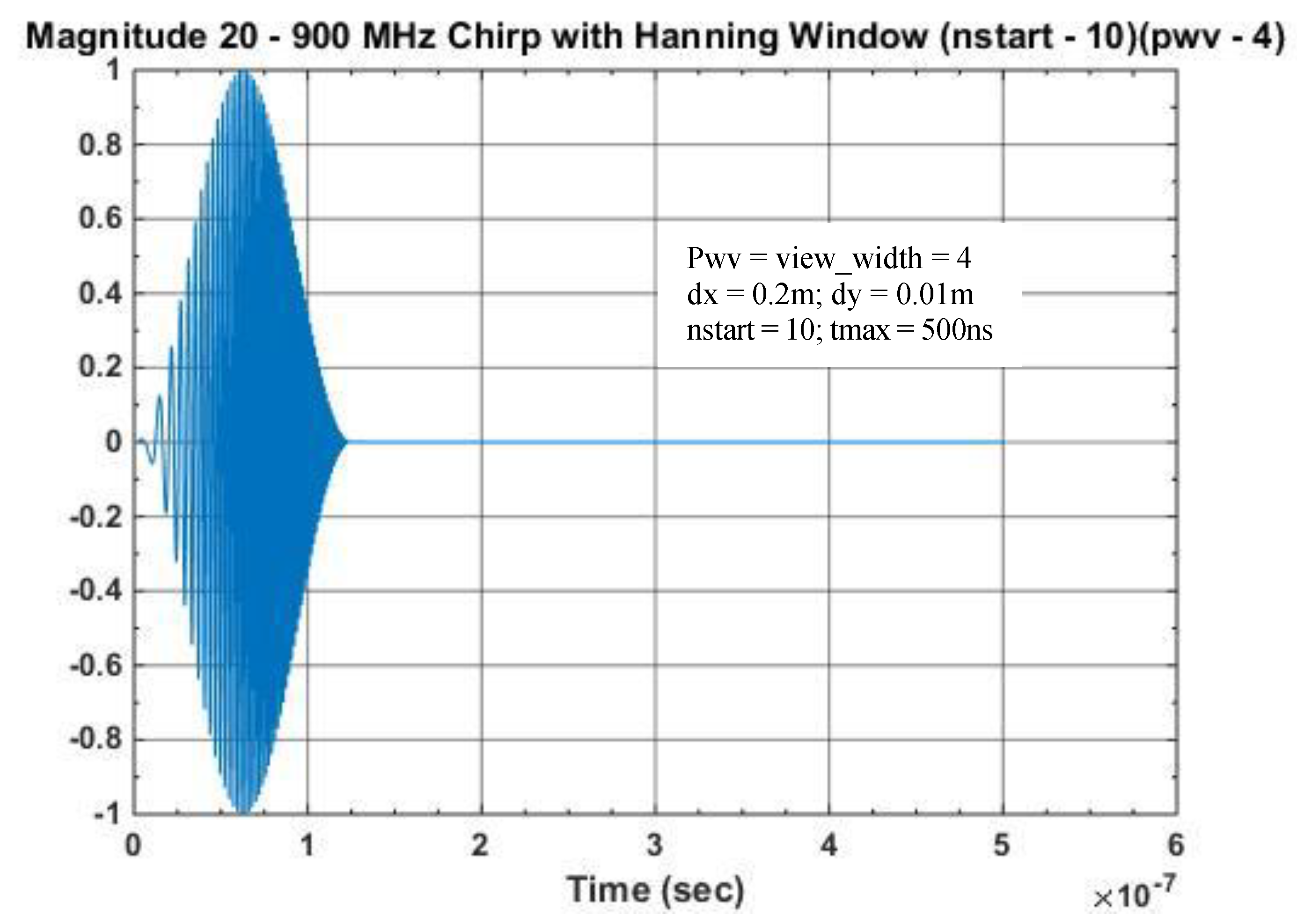
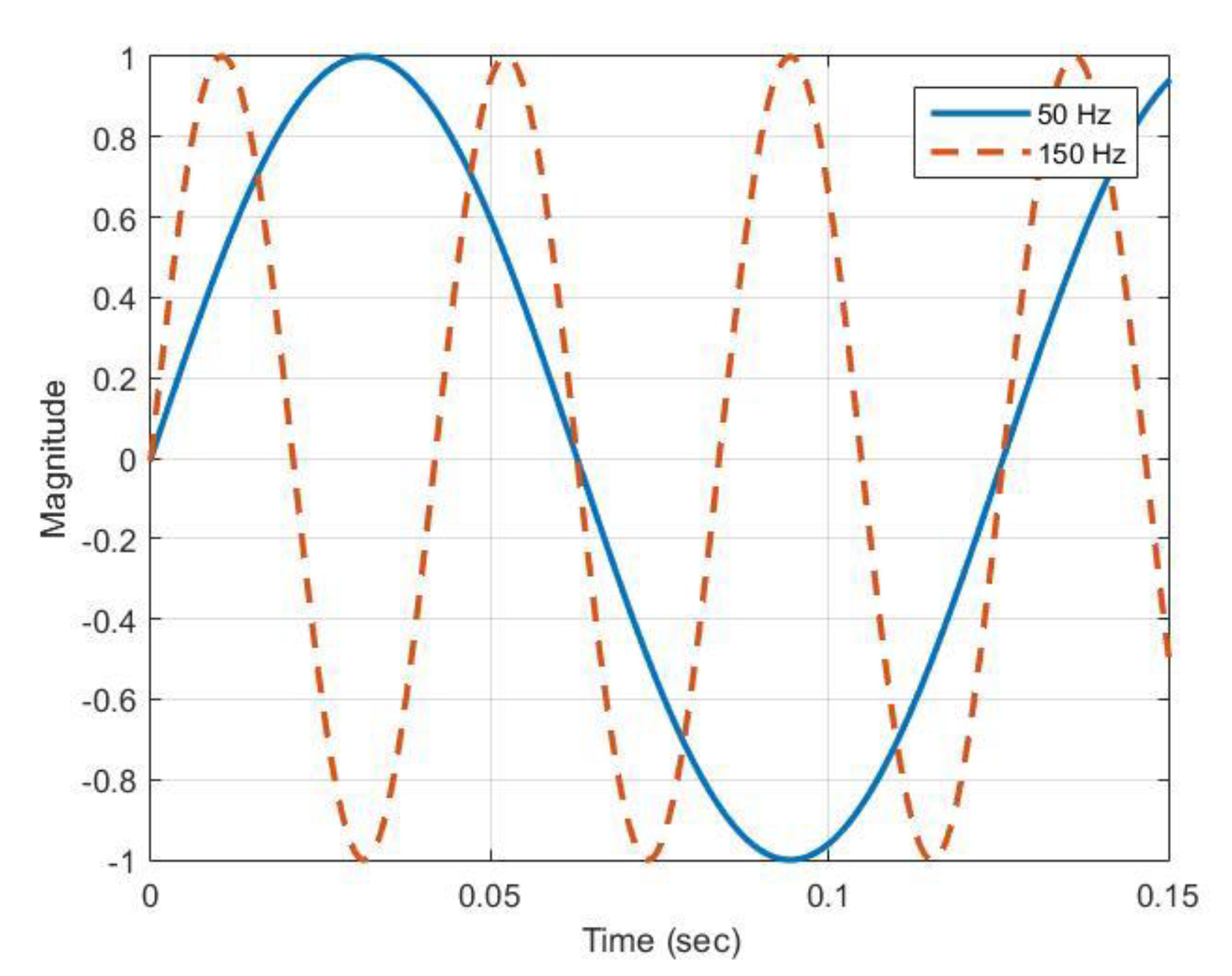
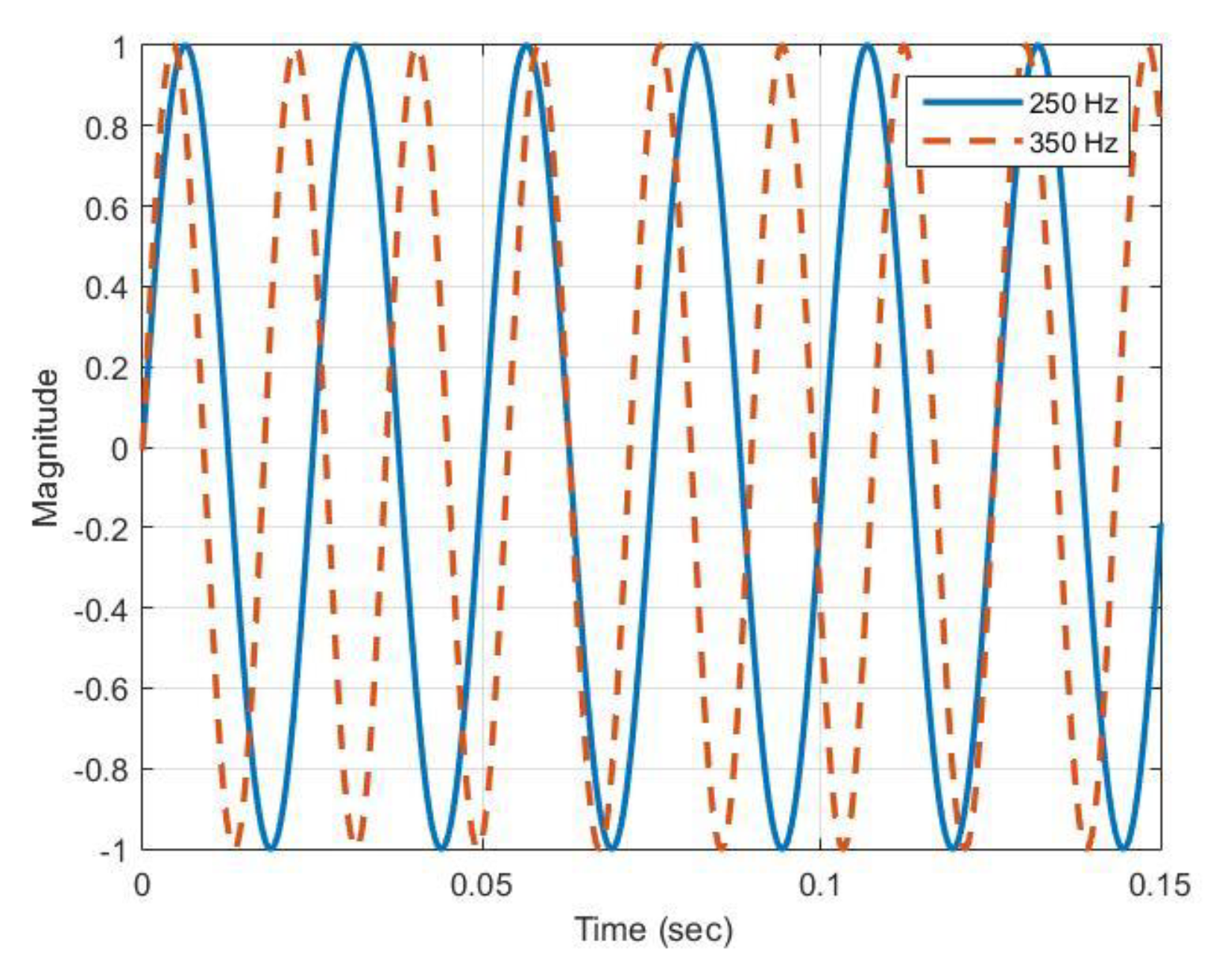
A signal in which the frequency increases with time or decreases with time is often named a chirp or sweep signal after the sound often made by birds. Creating a chirp excitation function-based radar signal, for use in this study, required computing a nominal chirp signal and deciding among several attributes. Increasing or decreasing chirp, exponential or linear, length of time the chirp signal is applied, the start time the chirp signal is applied, and the magnitude, are a few of the attributes requiring definition. For our study we chose an increasing linear chirp with a maximum amplitude of 1. Increasing linearly, in that the change from one frequency to the next frequency increases in a linear fashion.
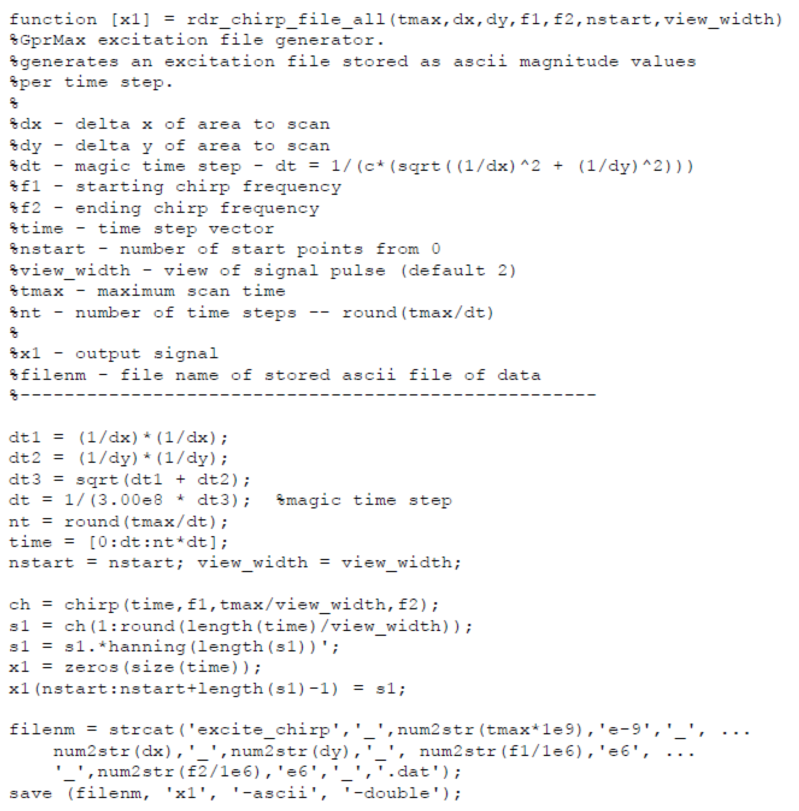
For use in the GprMax software program, we created sampled chirp signals structured to match each time step for the delta area (∆x and ∆y) of a 2-D analysis. We arbitrarily chose the length of time the chirp signal would be applied (view_width) as ¼ of the entire time the computer analysis was defined to run (tmax). The length of time was similar to that when a Ricker pulse signal is used in GPR analyses. The chirp start time was defined arbitrarily as 10 time samples. We implemented an added feature of using a Hanning window to soften the initial start and end of the created chirp pulse.
These choices were compiled and implemented in MATLAB code.
Figure 1, shows the code used and
Figure 2 shows the labeled result. The increasing linear chirp signal was designed to cover the frequencies used in the current EM analysis (20, 30, 50, 100, 500, and 900 MHz); consequently, the linearly increasing chirp start and end frequencies were defined as 20 MHz and 900 MHz, respectively. The frequency time step is not explicitly shown in the computer code of
Figure 1 but can be calculated using the following equation based on the variables defined in
Figure 1 and
Figure 2.
where:
c = speed of light (3 × 10⁸ m/s),
(∆x, ∆y)—2-D analysis defined delta area.
For the parameters defined in
Figure 2, the frequency step is 0.234 MHz. This value varies with the modeling area definition. The computer code is structured using the MATLAB standard routine “Chirp” to generate a basic chirp signal and the MATLAB routine “Hanning” to generate a Hanning window.
5. Results
To determine the capability of the chirp excitation function scans to replace the combination of individual frequency scans, using the EM GMM method, we ran the same analyses on three fictional areas with a chirp excitation signal instead of the frequency scans with six different frequencies. The original scans used frequencies 20, 30, 50, 100, 500, and 900 MHz, combined using the EM GMM method. The chirp signal used was a linearly increasing chirp from 20 MHz to 900 MHz, processed through a Hanning window, as shown in
Section 4,
Figure 2. The frequency step is not directly calculated by the MATLAB chirp routine but can be calculated using Equations (17) and (18). The frequency step varies with the length of time (tmax) the scan is active and the delta model area (∆
x, ∆
y). Simulation model areas were defined using the modeling software package GprMax by Giannopoulos [
8] via the finite-difference time-domain (FDTD) analysis method solution to Maxwell’s electromagnetic wave propagation equations for GPR. As previously reported [
1,
2,
3,
4,
5], only 2-D analyses were performed. However, the software is capable of 3-D analysis as well. We reported earlier [
1,
4] the concurrence between actual scan results and simulated scan results; a brief review is included in
Appendix A.1.
Appendix A.2 includes a brief review of a test case of the EM GMM process operation [
2,
4]. Examples were constructed to allow for various transmitter (Tx) and receiver (Rx) heights above ground for two different target types to be studied. Tx/Rx were always positioned at the equal heights, above ground, for each scan. Heights included 5, 10, 20, and 40 m. A total of three modeling areas were previously defined and re-examined here for comparison of the EM GMM method with the chirp excitation function method. The removal of the direct arrival and ground bounce signals allows for a better focus on the reflections from the buried targets. Removal of these signals is easily done in simulation. We remove these signals from the analysis by scanning with the target(s) in place first, then without the target(s) in place. We simply subtract the two results to achieve removal. The result is scaled to a max value of 1 and processed. The magnitude of each processed signal plotted is scaled to a value of 1. Our interest in constructing the modeling spaces, defined below, was to evaluate the responses at defined distances above ground in an air medium, simulating the use of an unmanned vehicle performing the GPR scans, attempting to reliably image unknown buried objects.
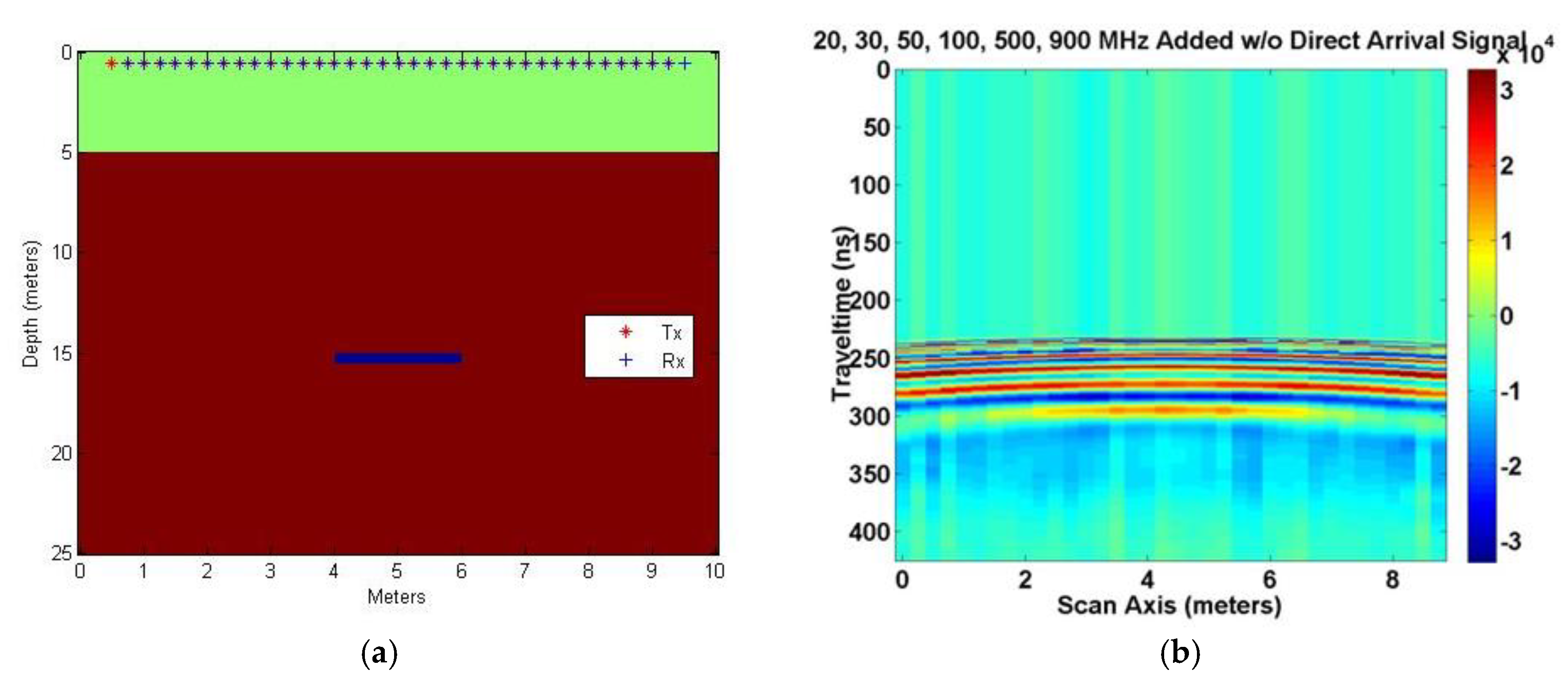
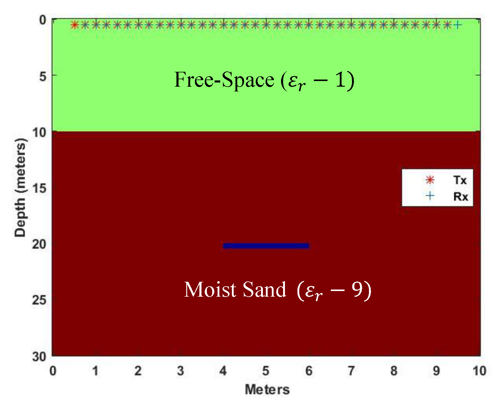
5.1. Defined Simulated Analysis Space 1
One defined area modeled consisted of a Tx/Rx positioned 5 m above the ground in air. The target is a perfect electrical conductor buried 10 m below the surface in a moist sand medium. Moist sand has a relative permittivity (
) of 9.0 and an electrical conductivity of 0.001 mS/m, where the velocity through the media is 0.1 m/ns. Free space or air has a relative permittivity of 1.0 and is considered “lossless” with an electrical conductivity of 0, where the velocity through the media is 0.3 m/ns. The defined space is labeled Simulated Analysis 1 (SA1). The target is 2 m in length and 0.5 m in depth. The model area is 10 m in width and 25 m in depth. The Tx/Rx pair was moved along the scan axis (x-axis) 0.25 m per step for a total of 36 scans. The Tx starts at 0.5 m ending at 9.5 m in the x direction. The Rx starts at 0.75 m ending at 9.75 m in the x direction. Each scan, at 425 ns in length, is long enough to receive a reflected signal from 24 m below the Tx/Rx pair in a combined medium of air and moist sand. SA1 has a grid space of 200 points in the x direction, (∆
x—0.05 m), and 500 points in the y direction, (∆
y—0.05 m).
Figure 3a [
2,
3,
4,
5] shows the model, Tx/Rx positions, and the target area.
Figure 3b [
2,
4,
5] shows the six signals combined by scaling each signal’s max value to the same magnitude with the direct arrival and ground bounce removed. The target reflection covers a broad area in depth from 240 ns to 320 ns (two-way travel time), a rough indication of the target depth. The two-way travel time reflects the increased length in signal travel, above the vertical distance, due to the ray refraction caused by dissimilar medium, air to moist sand, resolvable using Snell‒Descartes law of refraction.
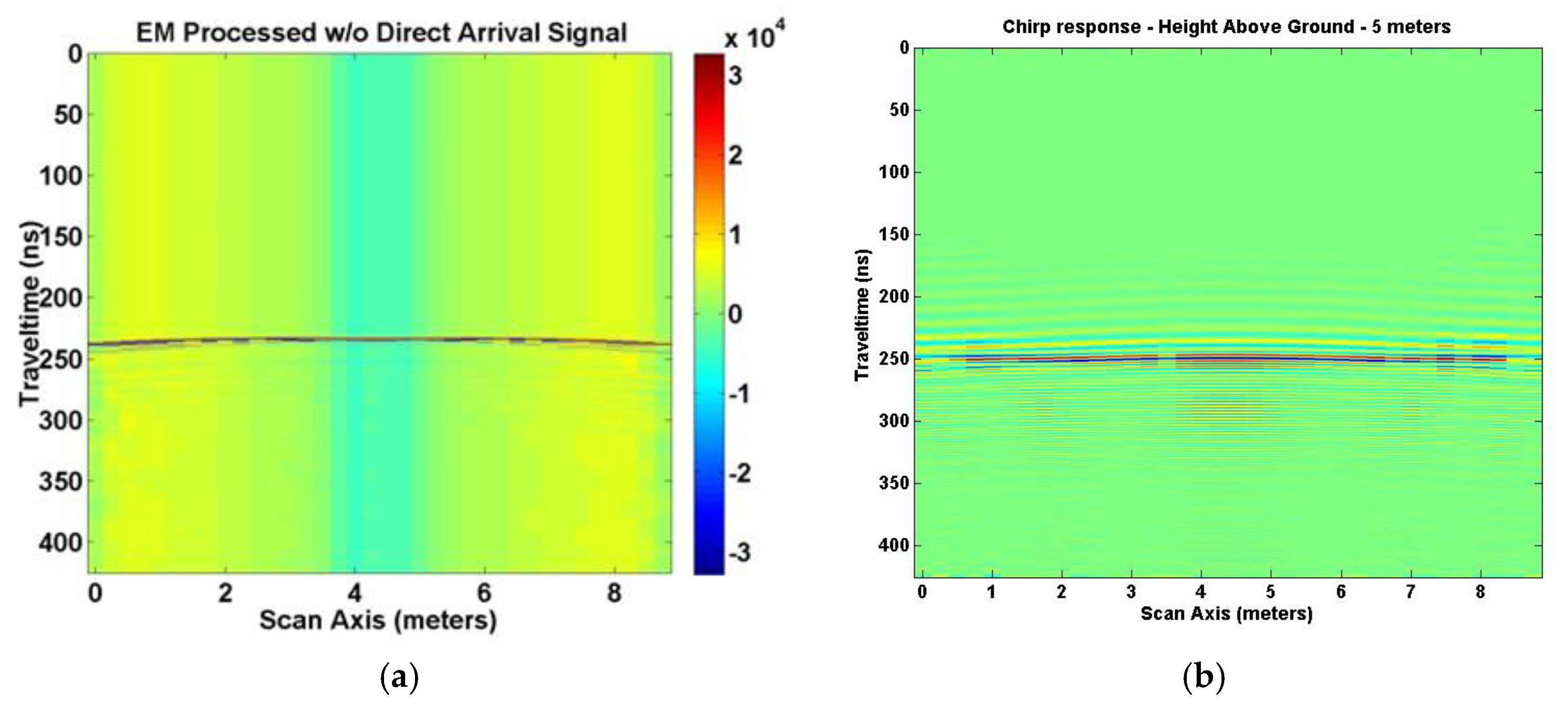
Figure 4a [
2,
3,
4,
5] shows the result from combining six different frequencies using the EM GMM method to determine the weight associated with each signal to be combined. The target is correctly shown approximately 15 m below Tx/Rx pair (240 ns), 10 m below ground.
Figure 4b shows the analysis result from the chirp excitation signal. The chirp result is not as broad as
Figure 3b [
2,
3,
4,
5] but it still more uncertain than
Figure 4a [
2,
3,
4,
5] with the same not well-defined edge detection of the target.
Though model SA1 has an area twice as deep as it has in width (bore hole), the analysis result is still valid and points to real differences in the techniques, EM GMM verses chirp excitation. A bore hole can be described as a very narrow width scanning area. The significance of the width is that the area scanned may not be wide enough to show the entire hyperbola, which normally forms above and around the object being scanned. This is occurring in
Figure 4. Adding to the problem is that hyperbola formation is affected by the length of the object and the depth. With the increase in depth and object length, the hyperbola tends to flatten out. Heights of 10, 20, and 40 m above ground with the same model SA1 features were examined to determine what other information, if any, might be realized.
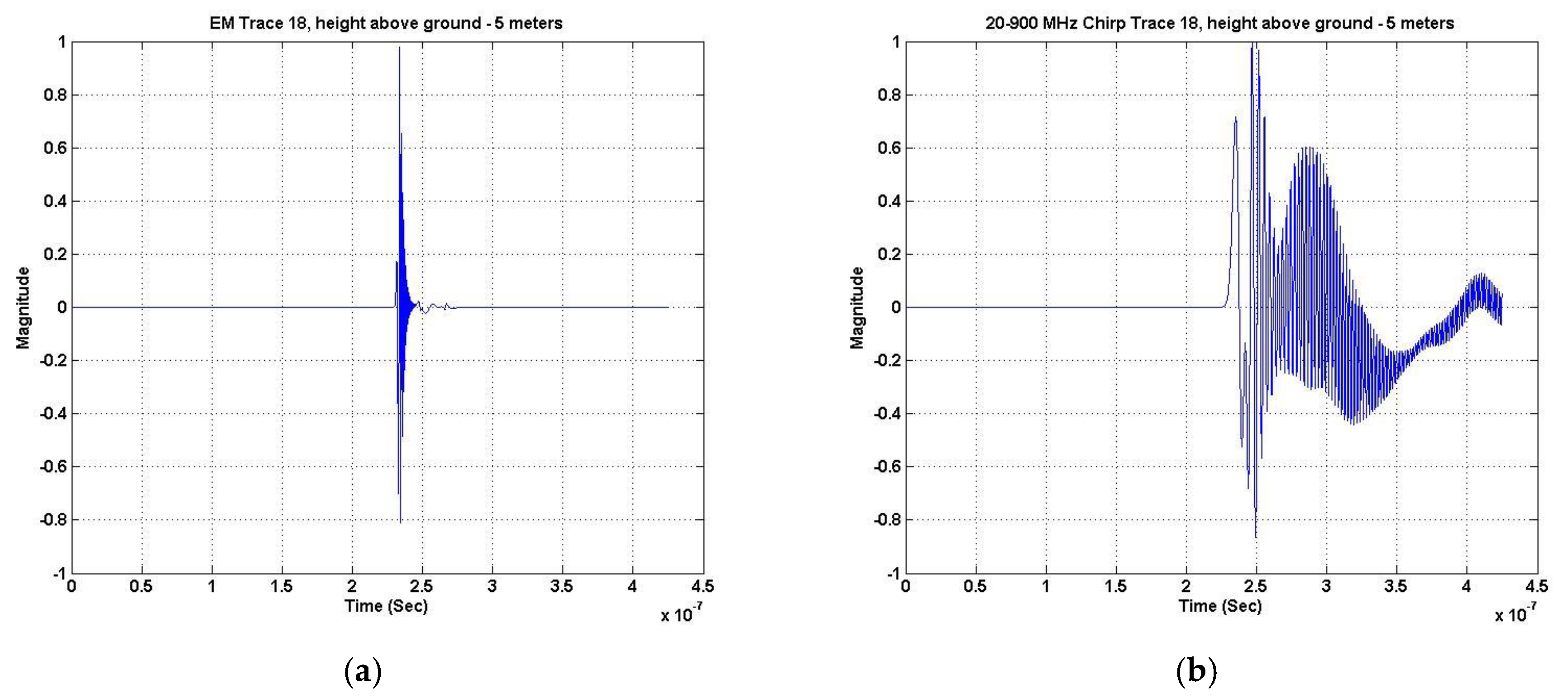
Figure 5 and
Figure 6 show and compare the 1-D plots of individual traces for the EM GMM analysis and chirp excitation analysis results at 5 m above ground.
Figure 5a shows the trace (18) at 5 m out of 10 m total in the x direction, roughly over the target for the EM GMM process.
Figure 5b depicts the same x direction trace for the chirp excitation analysis. The chirp trace is extended in time which is reflected in the multiple hyperbolas and target “ghosting” appearing in the image plot.
Figure 6 depicts traces at approximately 0.3 m (trace 1), 5 m (trace 18), and 8.3 m (trace 30). The EM GMM method produces a much tighter trace spread over the width of the scanned area (
Figure 6a). The chirp excitation response is noticeably broader (
Figure 6b). However, they both indicate a 240 ns two-way travel time, corresponding to a target at 15 m below the Tx/Rx pair. Of note is that the direct arrival and ground bounce signals have been removed.
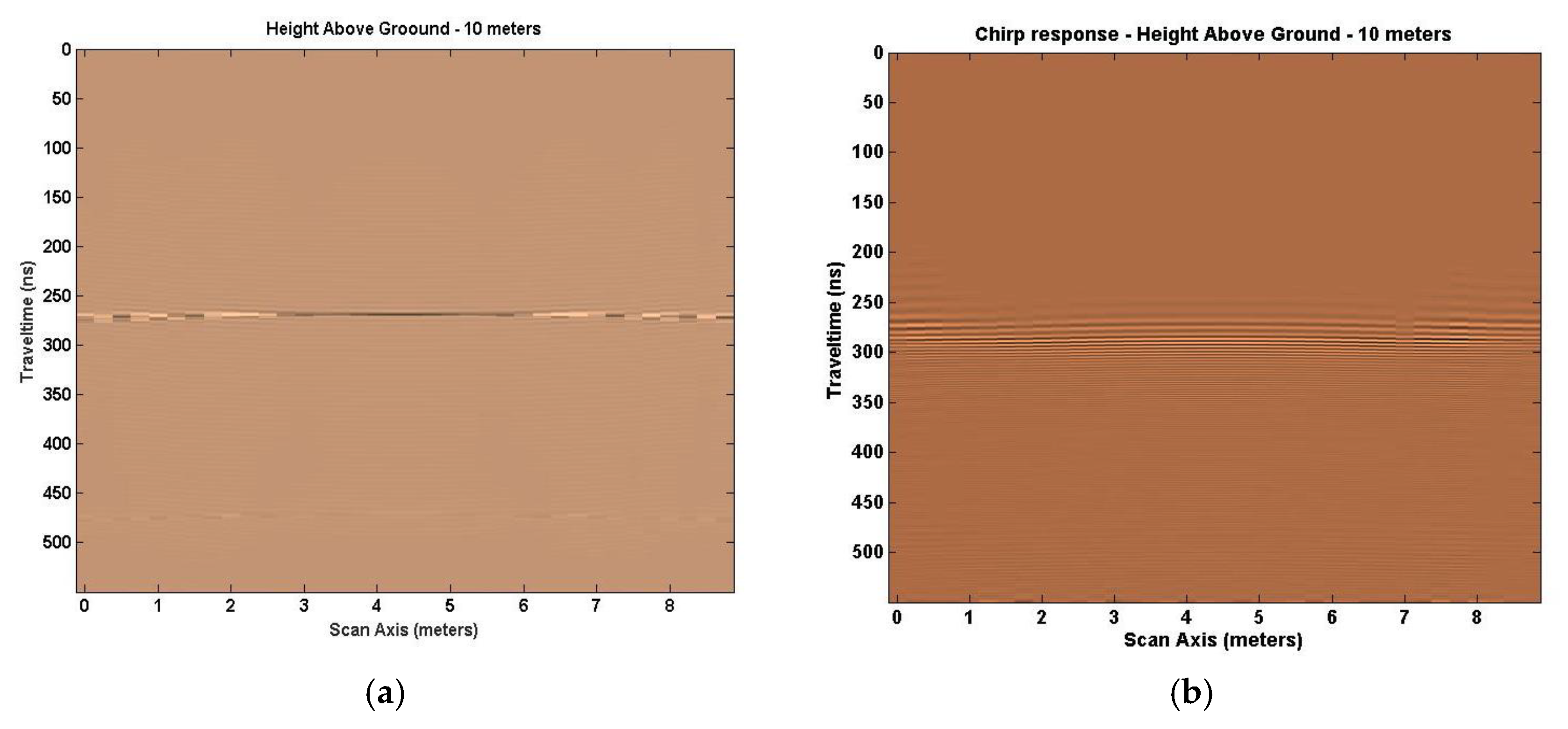
Figure 7 and
Figure 8 [
5] depict the changes to the SA1 defined space model and the GPR analysis result at 10 m in height above ground, respectively. The reflected GPR response shows the target at 20 m below the Txs and Rxs for a two-way travel time of 270 ns. The chirp response (
Figure 8b) is not as well defined in depth and the width suffers from the bore hole effect.
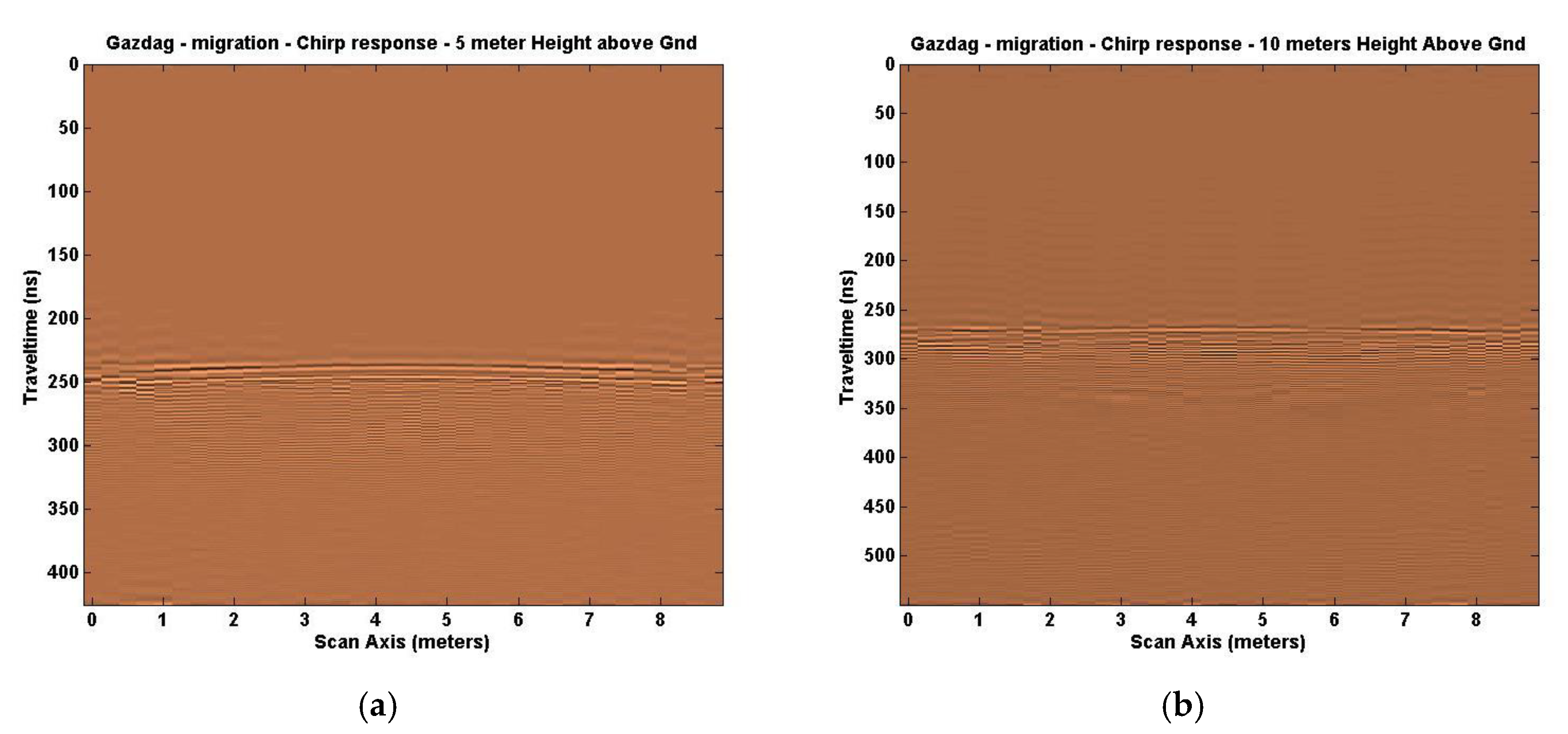
To compensate for geometric distortion of chirp waveform responses, we looked at using three methods: the phase shift migration method of Gazdag [
17], signal compression (correlation of received signal with transmitted signal), and filtering the received signal into six separate frequencies (the frequencies used in the EM GMM analysis), then using the result to calculate a EM GMM response. The Gazdag method [
17], like the Stolt [
16] and FK [
18,
19] techniques, attempt to account for phase shifts that occur when the angles the radar signals are sent from are different than the angle the signals are received. The change from the unprocessed chirp response to a Gazdag [
17] processed chirp signal is minimal but important. The signal echoes above the reflected target are reduced. Much was not expected because our transmit and receive angles do not change very much, especially for 2-D, so there is no azimuth correction to make.
Figure 9a depicts the response due to Gazdag [
17] for Tx/Rx pairs at 5 m in height above ground, and
Figure 9b depicts the response at 10 m in height above ground.
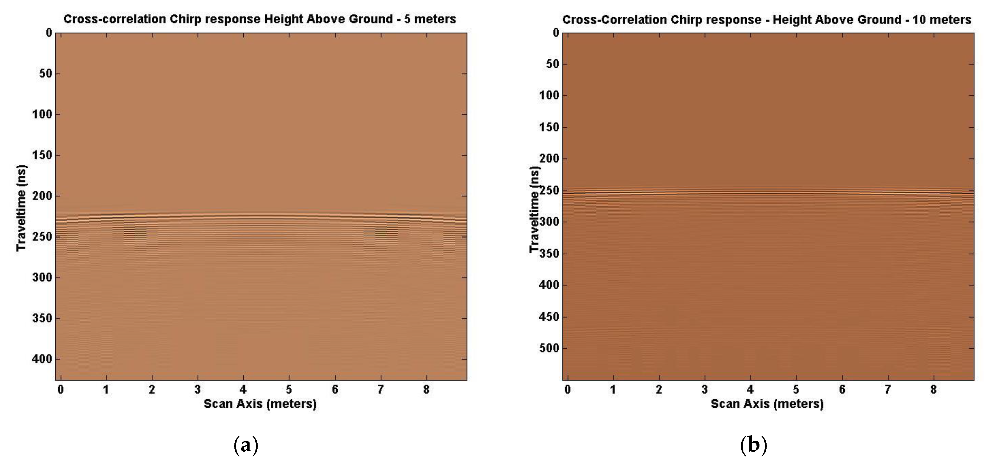
Figure 10 shows the result of correlating (cross-correlation) the transmitted signal with the received signal for Tx/Rx pairs at 5 m and 10 m above ground. Signal to noise enhancement is defined as the result. Multiple lines above the reflected target position are significantly reduced or non-existent, displaying an output closer to the EM GMM method response. Good edge detection and broadness in depth of the response is still less than desired.
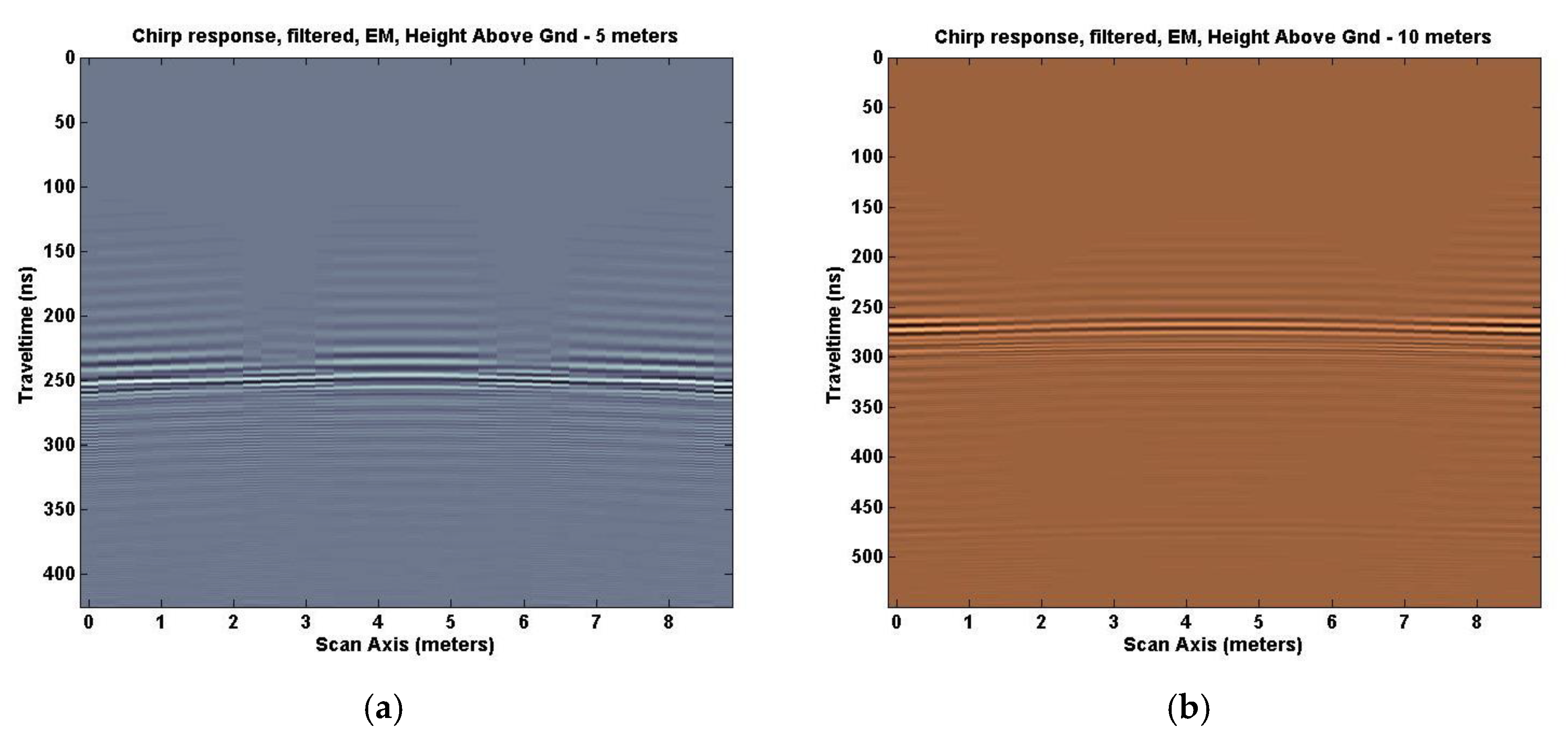
Figure 11 shows the result of filtering the original chirp excitation response with six different filters: a 20 MHz low pass filter, 30 MHz bandpass filter, 50 MHz bandpass filter, 100 MHz bandpass filter, 500 MHz bandpass filter, and a 900 MHz high pass filter to mimic the 6 frequencies used for the compositing process. Each section began with unit amplitude, then underwent the EM GMM process to determine the weights needed to combine these six frequency responses. The result was not as impressive as we would have liked. A multi-band reflection remained in the solution shown for Tx/Rx pairs at 5 m and 10 m above ground.
Further comparison results for Tx/Rx pair heights at 20 and 40 m were not included in this paper because no further conclusions were realized beyond the normal signal degradation as the target depth increased. Geometric distortion methods for this model space (SA1) were no longer considered for study, based on the above results.
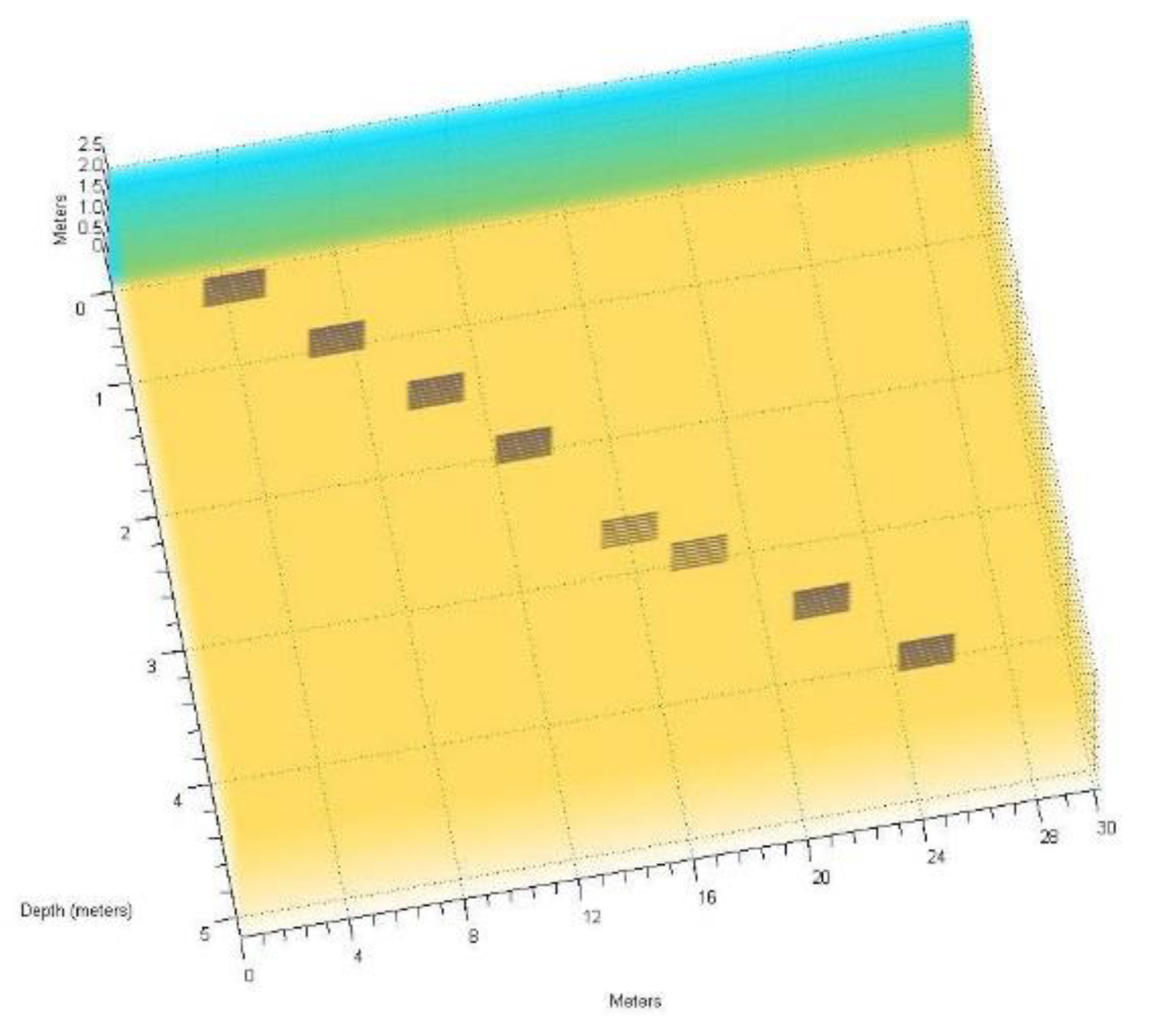
5.2. Defined Simulated Analysis Space 2
A more complicated set of targets were developed for follow-on analyses. The second defined space model developed (Simulated Analysis 2—SA2) consisted of an area 30 m in width and 25 m in depth with almost no space above ground (0.15 m) for the Tx/Rx pair. Eight targets were buried at eight different levels. These targets represent sheets of corrugated aluminum, modeled as perfect electrical conductors. Each sheet was approximately 2 m in length and 0.1 m in depth. The eight burial levels were 4.565, 6.065, 8.565, 10.065, 12.815, 14.065, 16.565, and 18.065 m. The odd metric values are due to a not well-defined start burial level of approximately 15 ft deep (4.565 m). Each additional increase in depth was computed in meters (1.5, 2.5, 1.5 m, etc.). The sheets were buried in dry sand with a relative permittivity (
) of 3.0 and electrical conductivity of 0.001 mS/m, with a velocity through the medium of 0.1732 m/ns. The Tx/Rx pairs were swept along the scan axis with the Tx starting at 0.5 m and ending at 24.85 m. The spacing between a Tx and Rx remained at 0.25 m. Each scan is 550 ns long and capable of receiving a reflected signal from roughly 48 m below each Tx/Rx pair in dry sand. The model grid space is 150 points in the x direction (scan axis: ∆
x—0.2 m) and 2500 points in the y direction (depth axis: ∆
y—0.05 m). Scanning frequencies for the EM GMM response are the same as before (
Section 5.1). The chirp excitation function and frequency step changed as calculated using the software program in
Figure 1 and Equations (17) and (18), respectively, detailed in
Section 4. The direct arrival and ground bounce signals were removed as before (
Section 5.1).
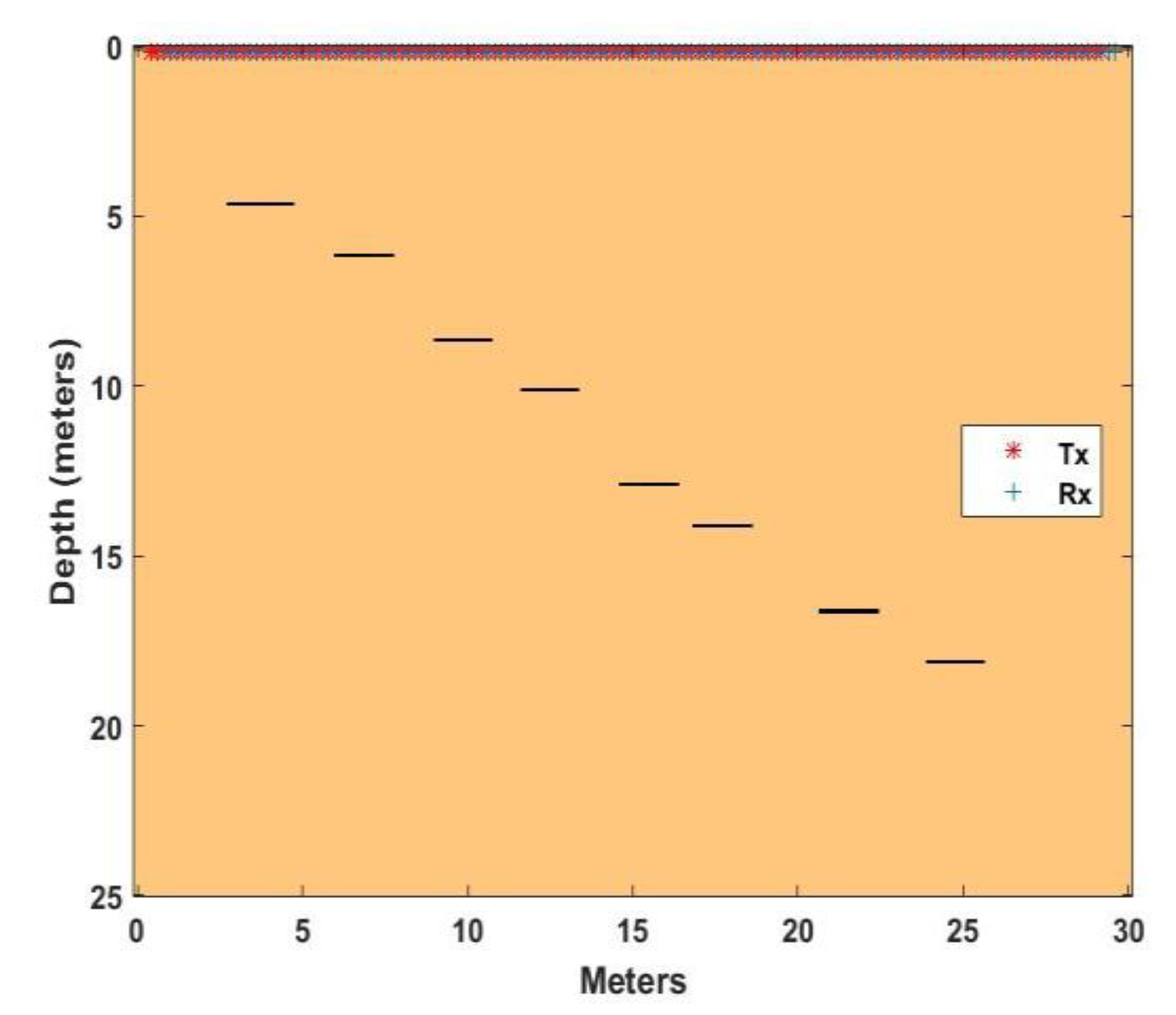
The model SA2 is shown in
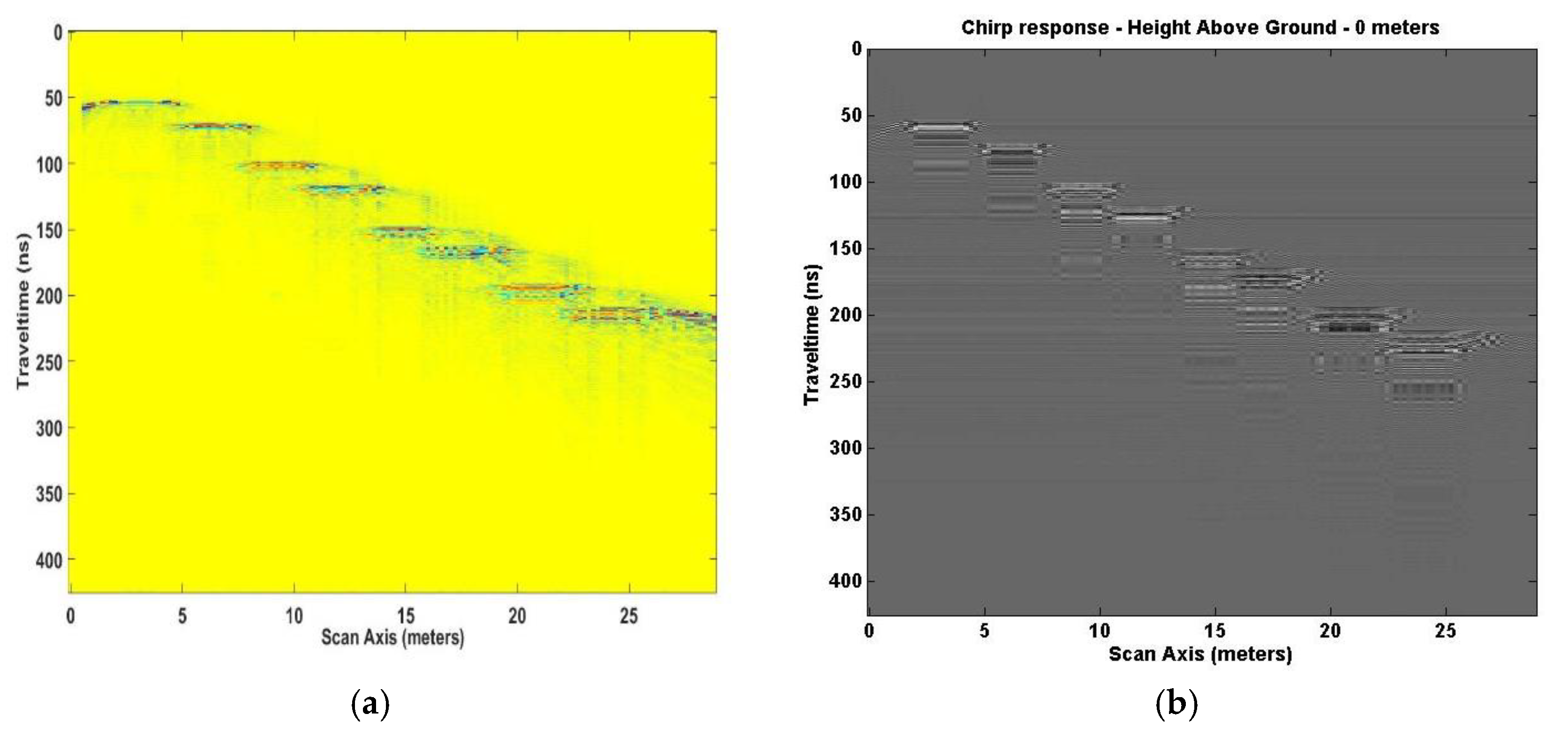
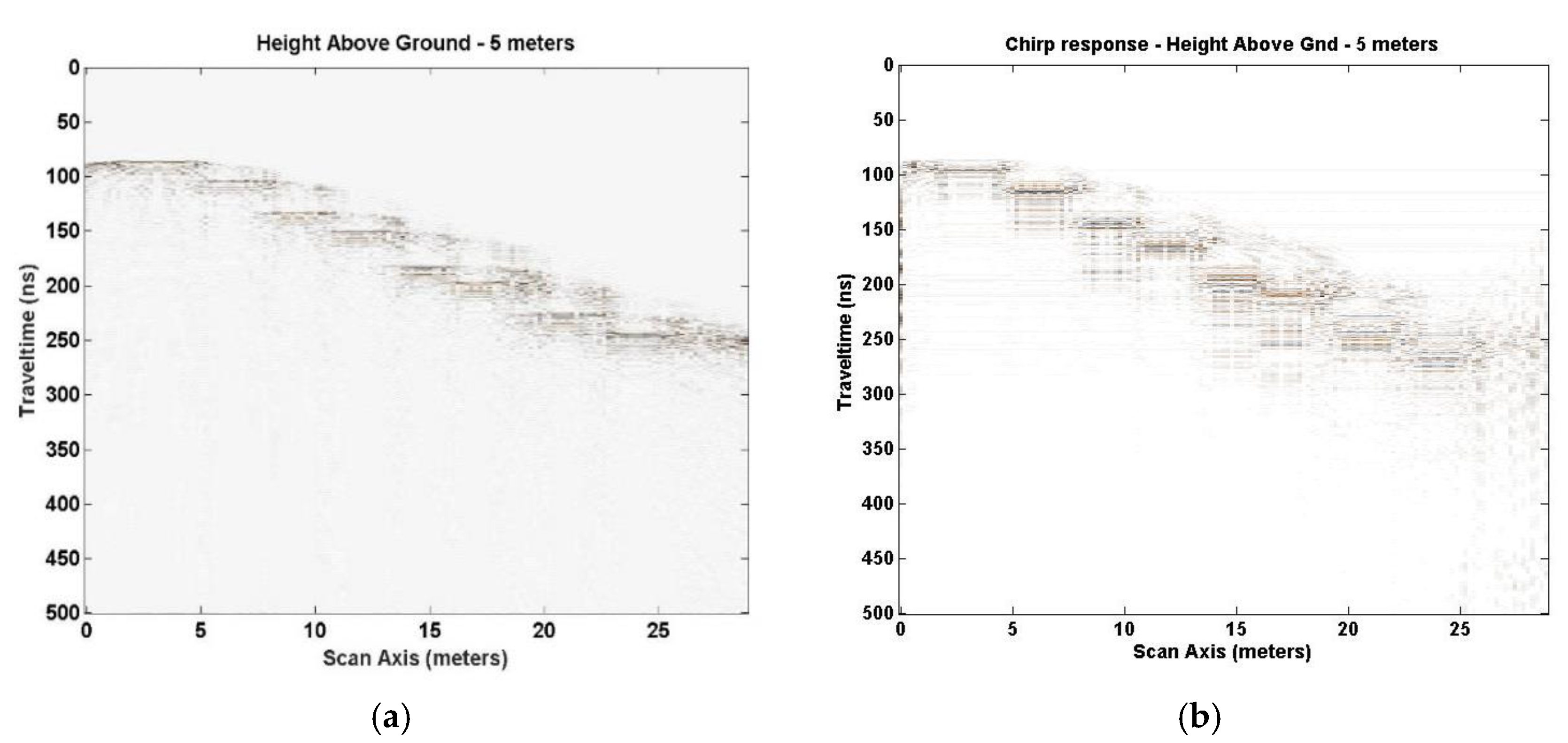
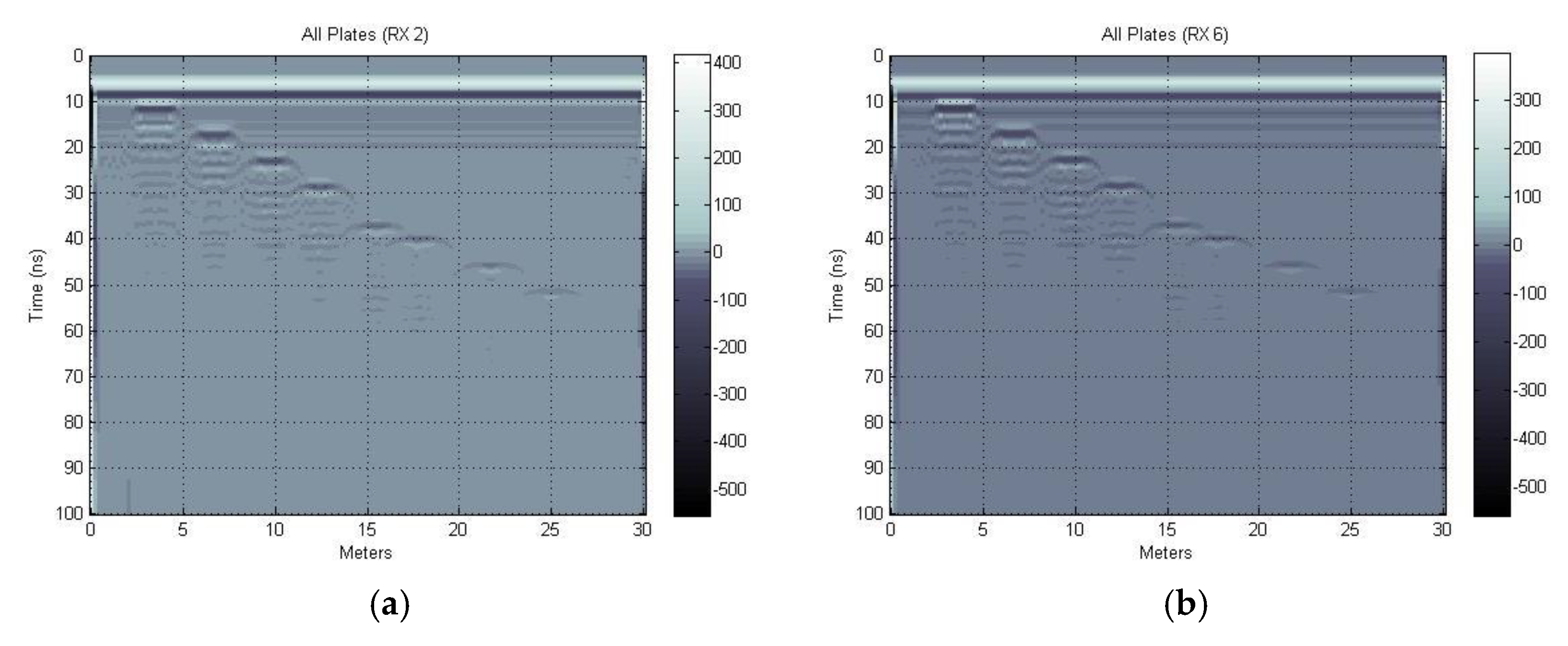
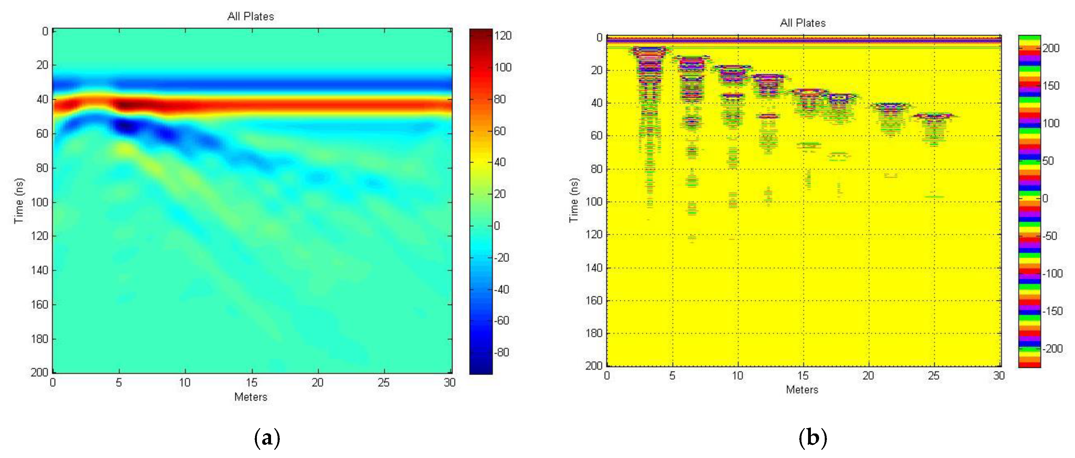
Figure 12. The result from the EM GMM method, shown in
Figure 13a, correctly depicts the depths of the sheet targets at approximately 50, 70, 100, 116, 148, 160, 190, and 208 ns for two-way travel time.
Figure 13b depicts the chirp excitation function response and shows better edge detection capability, while
Figure 13a shows better depth delineation. The same result was found previously in the model SA1 studies.
We repeated the analysis for a Tx/Rx pair at a height of 5 m above ground in free space.
Figure 14 shows the SA2 model used for the analysis.
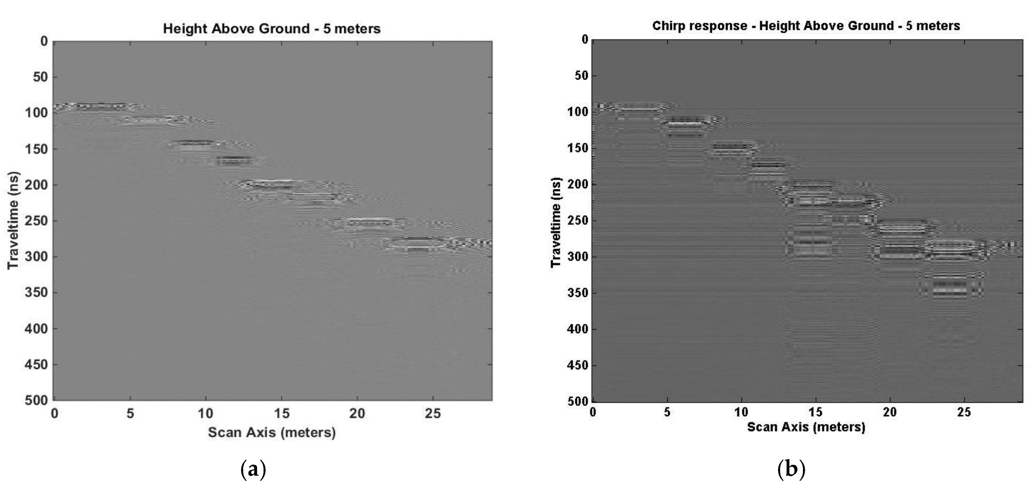
Figure 15a shows the response with the EM GMM method, and
Figure 15b shows the chirp excitation signal response. Again, the chirp signal response displays good edge detection but coarse depth detection. Each method detects eight objects but not clearly. The chirp result shows eight “ghost” reflections underneath eight objects.
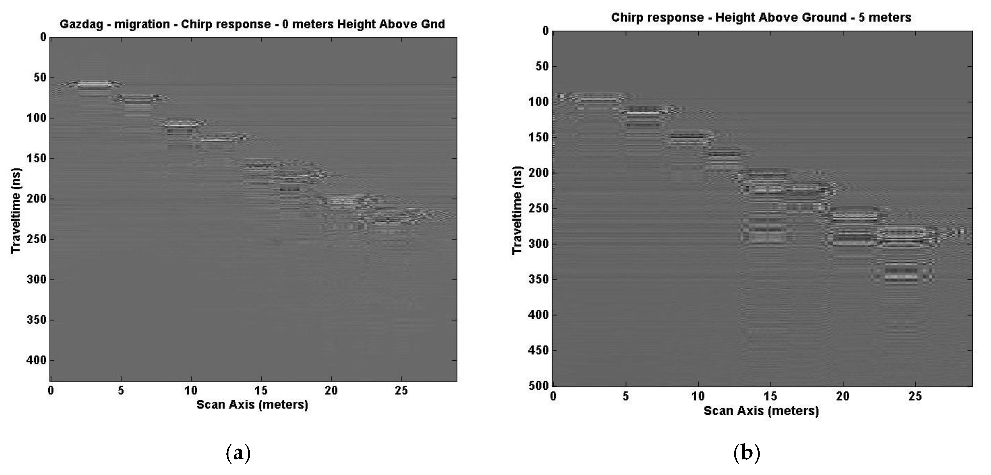
We repeated a look at compensation methods for geometric distortion of chirp waveform responses that we explored in
Section 5.1., i.e., Gazdag migration [
17], correlation, and separating the response by filtering with six separate filters then compositing the result using EM GMM.
Figure 16 shows the Gazdag [
17] result for a Tx/Rx pair at approximately 0 m (0.15) and 5 m height above ground. Except for the more noticeable “ghosting” below each recognized target, the change from
Figure 15b is barely noticeable in
Figure 16.
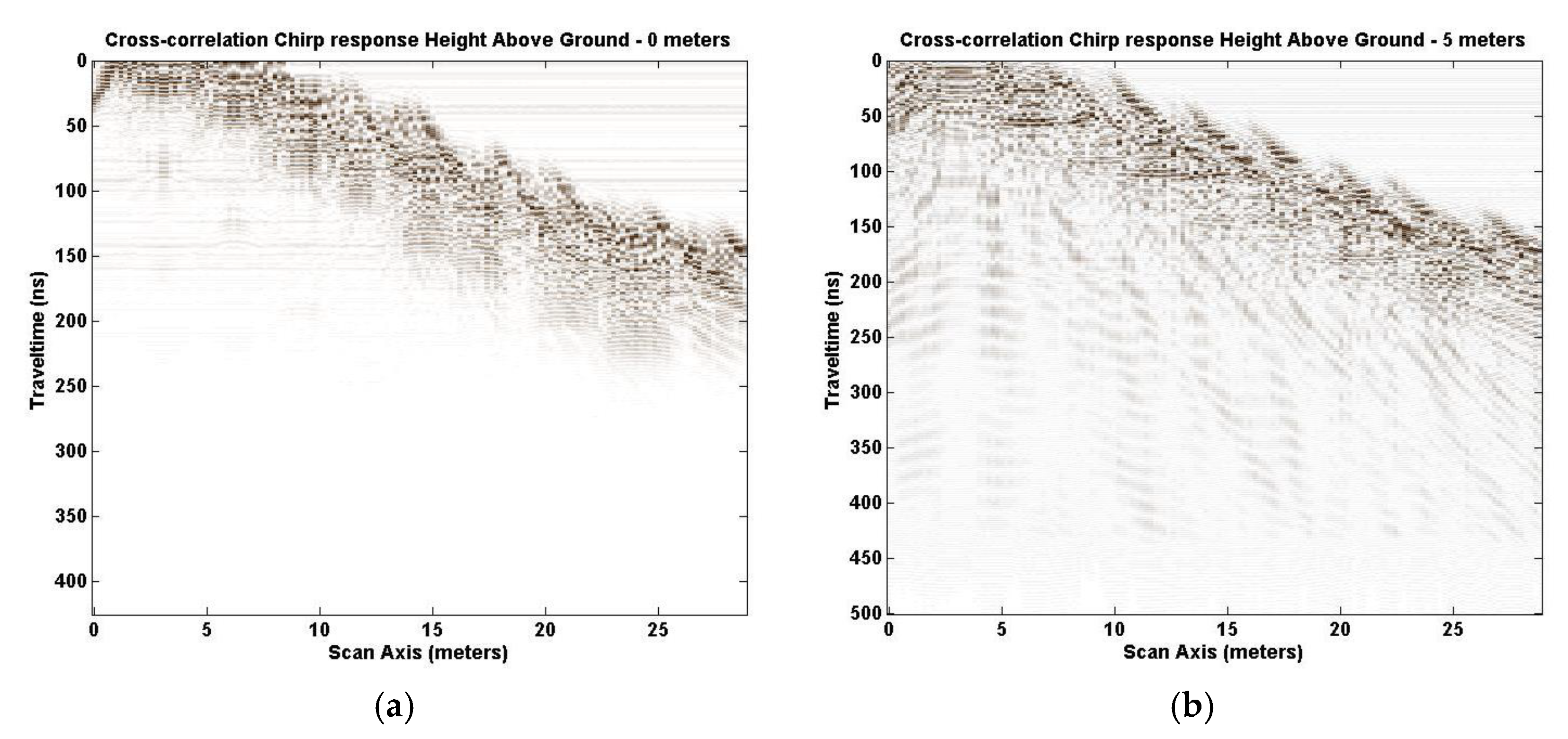
Figure 17 shows the result after correlating the transmitted signal with the received chirp signal with a Tx/Rx pair at approximately 0 m (0.15) and 5 m. With migration the output is a bit more cluttered, and with correlation much more clutter is evident. In
Figure 17, about all that can be determined is that there are objects proceeding in a downward stair-step fashion as one moves along the x axis (scan axis) with at least eight concentrated reflections underneath at least eight objects.
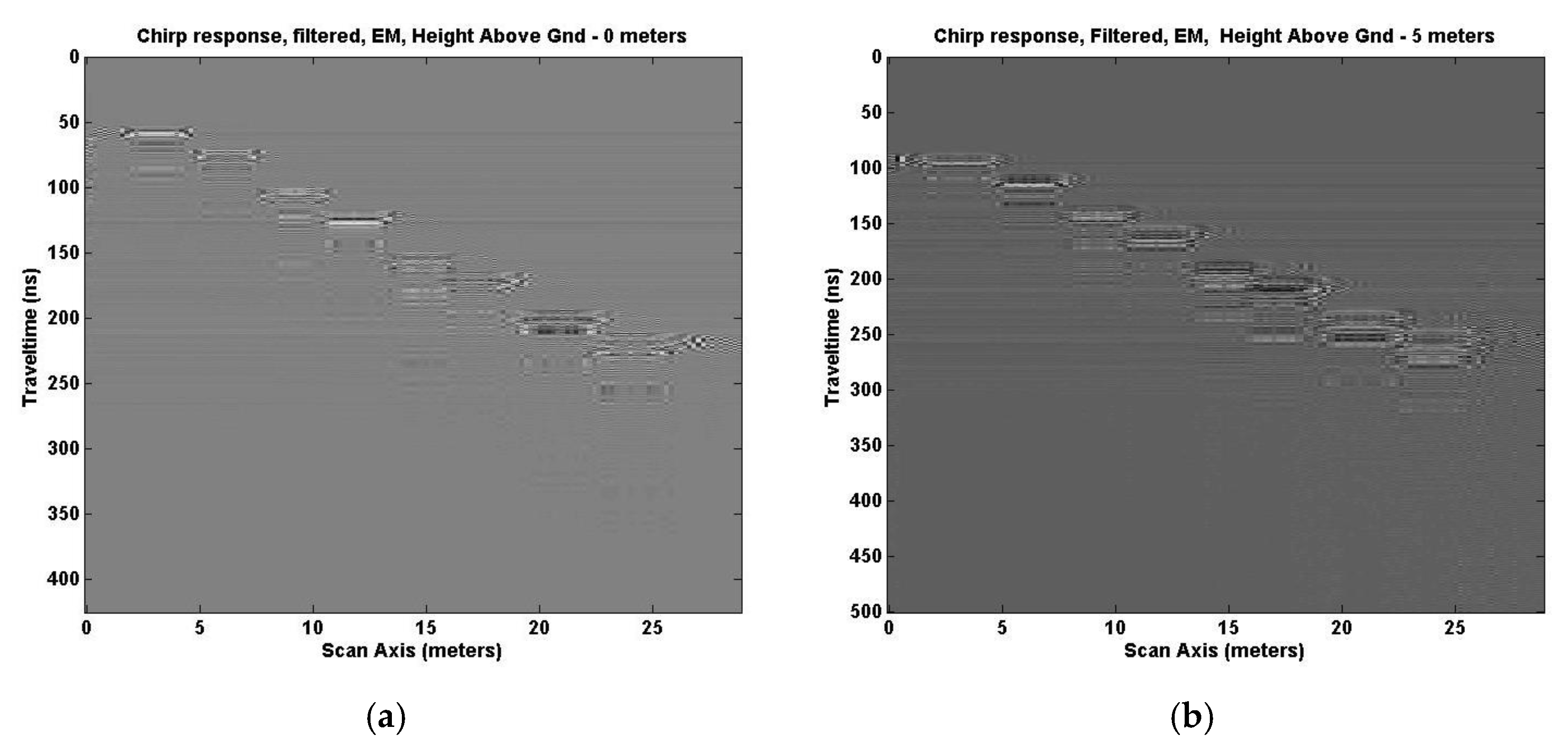
Filtering the original chirp excitation response into six separate frequencies then using the EM GMM process to combine them is shown in
Figure 18 at heights of approximately 0 m (0.15) and 5 m for a Tx/Rx pair. There is very little change in response of the chirp excitation images using this filtering technique, certainly not enough to routinely apply this feature to the data received. The multiband reflection at each target object remains and is possibly enhanced making the image a bit less clear. The results are similar to the SA1 model case of
Section 5.1. EM GMM scanning comparison results with chirp excitation responses for Tx/Rx heights of 10, 20, and 40 m do not appear in this paper because no further conclusions were realized beyond the normal signal degradation as the target depth increased.
5.3. Defined Simulated Analysis Space 3
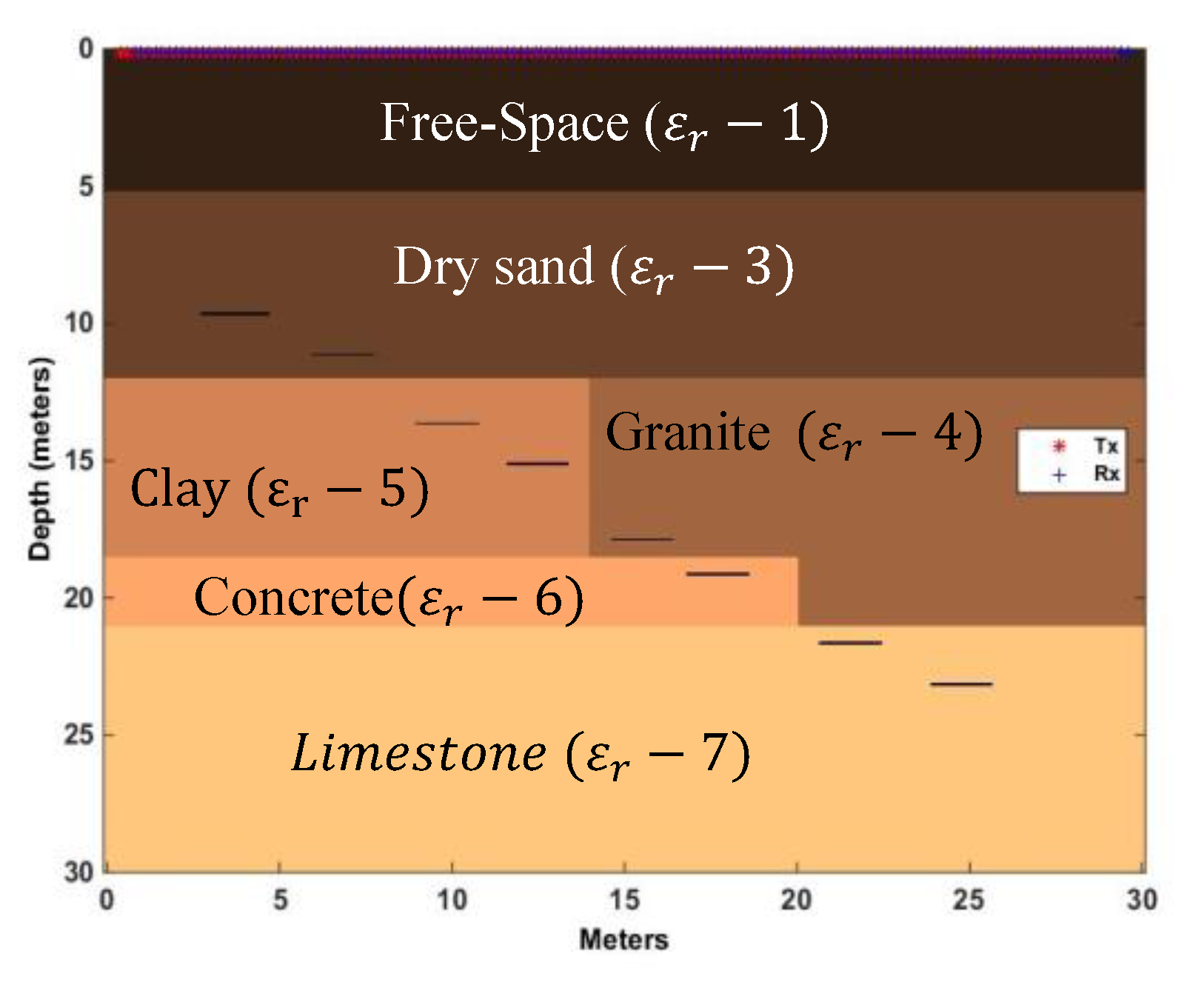
We developed a third defined space model labeled SA3 (Simulated Analysis 3) using the same area dimensions and target designations of the SA2. The SA3 model placed the target objects in non-homogenous materials instead of the homogenous materials used in SA1 (moist sand) and SA2 (dry sand). A model area was created with dry sand, clay, concrete, granite, and limestone with a relative permittivity (
) of 3.0, 5.0, 6.0, 4.0, and 7.0, respectively, noted in
Figure 19. The velocity through each medium is 0.1732 m/ns (dry-sand), 0.1342 m/ns (clay), 0.1225 m/ns (concrete), 0.1500 m/ns (granite), and 0.1134 m/ns (limestone). In
Figure 19 there are coloration differences to denote the different media used in the model. As before, the EM GMM response is observed side by side to the chirp excitation function response and the same frequencies are used in the analysis. The study was conducted for Tx/Rx heights of 5, 10, 20, and 40 m above ground, however, responses at 10, 20, and 40 m are not included or discussed in this paper; no new information is realized beyond signal degradation as target depth increases.
Figure 19 depicts the SA3 model with Tx/Rx pairs 5 m above ground.
Figure 20a shows the EM GMM response, while
Figure 20b depicts the chirp excitation function response. The results are similar to those discussed earlier among the SA2 model results.
Figure 20a continues to have the edge detection problem with minor reflections under each of the eight objects.
Figure 20b continues to show better edge detection but much larger reflections under each of the eight objects, some large enough to be considered objects in themselves and not “ghost” reflections. Again, no further conclusions are realized over the SA2 model cases except for the signal loss due to the different media of the SA3 model. Results of scans at 10, 20, and 40 m were not included in this paper because new findings have not been identified besides the normal signal degradation that occurs as the buried target depth increases.
6. Conclusions
In this paper, we explored the idea that perhaps a chirp excitation function could replace the six frequency GPR scans combined using the EM GMM method reported earlier in references [
1,
2,
3,
4,
5]. This idea was bolstered by
Section 2 (related work) discussions on chirp signals in SAR [
9,
10,
11] systems and ground-based methods, such as vibroseis [
12,
13,
14,
15], where Gazdaq migration and compression techniques enhanced chirp received signals. In reviewing EM compositing methods using maximum-likelihood techniques, we determined that the path to better detection was strengthened by the number of times an area was scanned to collect enough data for compositing of signals. We used six frequencies in our earlier studies encompassing a broad range of frequencies (20, 30, 50, 100, 500, and 900 MHz) to image a broad range of targets at different depths. The task we set out to accomplish was to create a chirp excitation signal to replace these six frequencies using the previously defined analysis spaces, media and buried targets.
To that end, we created a linearly increasing chirp excitation signal starting at 20 MHz and ending at 900 MHz. The chirp signal was designed to match each time step created by the previous EM GMM analyses corresponding to the ∆
x and ∆
y grid space for a defined model area containing buried targets. The chirp pulse was applied only ¼ of the length of time for a single scan to allow for fewer interference reflections from the area being scanned. This length of time is similar to the Ricker pulse excitation function. The Ricker function equation is such that as time increases the magnitude decreases after its maximum value is reached. Using the software program GprMax [
6], we repeated the same analyses, previously run with the six individual frequencies, with the generated chirp signal data. The EM GMM method and chirp method results were compared side by side for heights 5, 10, 20, and 40 m, for the same buried targets and media types. The chirp-based GPR response was processed in the same manner as the EM GMM signals; the direct arrival and ground bounce signals were removed before processing further. For the EM GMM case, compositing occurred then the image was plotted. For the chirp case, just the image was plotted. The end product (GPR image plot) was better than we expected for the chirp excitation method but not as good as the EM GMM method. We found that although the edge detection capability of the end product was greatly improved by the chirped response signal, the depth indication was broader. This result was repeated when we added the six frequencies without searching for the best weighted combination; something the EM GMM process does routinely. We found this time and previously that the EM GMM method performed edge protection very poorly, but depth detection very well; very little “ghosting” occurred [
1,
2,
3,
4,
5].
Taking a page from the SAR processing notebook, we decided to explore the result of correlating the chirp output response with the chirp input signal. This normally produces a better signal-to-noise ratio for the received signal, clearing up noise related problems. That outcome (noise reduction) occurred where multiple lines above the designated target position were significantly reduced but the broad depth indication remained. We implemented Gazdaq [
17] migration with the thought that we had a phase shift problem. The result was less effective than the correlation process. The indication was that our 2-D analysis did not have a phase-shift problem.
We repeated chirp, Gazdaq [
17], and correlation processes on a more complicated defined space with the same results. We further performed the chirp process on a non-homogenous media defined space, producing the same outcome with some signal degradation due to non-homogenous media interfaces. The EM GMM method remained the superior method, though it would require more passes over an object to achieve good target detection. We showed that, unless one needed the increased resolution, just a chirp excitation signal was good enough to get a coarse idea of the location of buried targets. We concluded, from actual plots, that as the target depth increased, no new information was discovered, so those records were not included in this paper (depths greater than 20 m for SA1 defined space and 10 m for SA2 and SA3 defined spaces).
Problem areas remaining to be addressed are better edge detection techniques, removal of direct wave and ground bounce signals, and how to best align GPR trace starting points across frequencies being used for compositing. We speculate that solving this alignment problem just might reduce the thickness in depth of the scan results. For removal of direct wave and ground bounce we ran each analysis with buried targets in place, then ran the same analysis without the buried targets in place, subtracting the two runs, producing the result we used for further processing.


