Change Detection in Remote Sensing Images Based on Image Mapping and a Deep Capsule Network


1
Key Laboratory of Intelligent Perception and Image Understanding of Ministry of Education, International Research Center for Intelligent Perception and Computation, Joint International Research Laboratory of Intelligent Perception and Computation, School of Artificial Intelligence, Xidian University, Xi’an 710071, China
2
School of Computer Science and Technology, Xidian University, Xi’an 710071, China
*
Author to whom correspondence should be addressed.
Remote Sens. 2019, 11(6), 626; https://doi.org/10.3390/rs11060626
Submission received: 24 January 2019
/
Revised: 25 February 2019
/
Accepted: 28 February 2019
/
Published: 14 March 2019
(This article belongs to the Special Issue Change Detection Using Multi-Source Remotely Sensed Imagery)
Abstract
:Homogeneous image change detection research has been well developed, and many methods have been proposed. However, change detection between heterogeneous images is challenging since heterogeneous images are in different domains. Therefore, direct heterogeneous image comparison in the way that we do it is difficult. In this paper, a method for heterogeneous synthetic aperture radar (SAR) image and optical image change detection is proposed, which is based on a pixel-level mapping method and a capsule network with a deep structure. The mapping method proposed transforms an image from one feature space to another feature space. Then, the images can be compared directly in a similarly transformed space. In the mapping process, some image blocks in unchanged areas are selected, and these blocks are only a small part of the image. Then, the weighted parameters are acquired by calculating the Euclidean distances between the pixel to be transformed and the pixels in these blocks. The Euclidean distance calculated according to the weighted coordinates is taken as the pixel gray value in another feature space. The other image is transformed in a similar manner. In the transformed feature space, these images are compared, and the fusion of the two different images is achieved. The two experimental images are input to a capsule network, which has a deep structure. The image fusion result is taken as the training labels. The training samples are selected according to the ratio of the center pixel label and its neighboring pixels’ labels. The capsule network can improve the detection result and suppress noise. Experiments on remote sensing datasets show the final detection results, and the proposed method obtains a satisfactory performance.
1. Introduction
With the development of satellite technology, the amount of remote sensing images can be acquired in the same region at different times easily. There are different kinds of remote sensing images obtained by different imaging sensors. Imaging sensors contain some types of remote sensing data such as very high resolution (VHR) images [1,2], multi-spectral [3] or hyperspectral images [4], synthetic aperture radar (SAR) images [5], polarimetric synthetic aperture radar images [6], etc. In this paper, we mainly focus on the change detection of SAR images and general optical images. These images are convenient to acquire and are commonly homogeneous and heterogeneous images for experiments.
Change detection is defined as the process of identifying variations of an object or a phenomenon by observing it at different times [7]. Change detection is applied in many fields [8,9,10]. According to the two acquired images [11], where the region is changed and where the region is not changed can be found through comparison. For these two images, many image preprocessing technologies including denoising and coregistration technologies are applied to deal with the data, aiming at decreasing the noise and making these images easy to compare [12]. These technologies are necessary owing to the existence of speckle noises [13]. These speckle noises may cause false alarms. Coregistration technology aims to place those pixels in a suitable position, namely a one-coordinate system [14]. Changed and unchanged regions are detected after comparing and analyzing the preprocessed images.
In general, the final resulting map contains two sorts of pixels, black and white, representing unchanged and changed regions, respectively. The change detection image result can reveal where the changed region is and whether the region is changed. We can find it by experiments instead of going to the location, which improves the efficiency greatly. There are currently two main change detection directions: one is homogeneous image change detection, and the other is heterogeneous image change detection [15,16,17].
Homogeneous image change detection is the change detection on remote sensing images in the same or a similar feature space. SAR images are traditional experimental data of homogeneous image change detection. The pixels in homogeneous images possess the same or a similar property or we can say that they are linearly related. They are easy to compare. Thus, many methods are applied in comparing these two images directly, such as the log-ratio method [18,19], the difference method [20], and the mean-ratio method, and other traditional ways have been put forward. They can generally achieve a fairly good performance. Usually, homogeneous image change detection can be performed in two ways. In short, one is to compare first and then to perform classification, while the other one is to classify them into different types and then compare. The classification often can be done by threshold segmentation methods like the Kittler and Illingworth (KI) [21] threshold method, the Otsu threshold method [22], and some other auto-threshold segmentation methods or some clustering methods such as FCM and K-means [23,24]. We can usually obtain a fairly good result, but there are many noises polluting the image. Then, a common way is to take the difference image as the training labels and input them into a neural network such as a convolutional neural network (CNN) [25,26], a generative adversarial net (GAN) [27], a deep neural network (DNN) [28], a deep belief network (DBN), a restricted Boltzmann machine (RBM) [29], etc. We can calculate the similarity level and obtain the ratio of the center pixel label and its neighboring labels to select reliable training samples [28].
However, we may meet a more complex situation in which two images are in different feature spaces. Some remote sensing images are less costly, and these images are not always taken from one kind of satellite. They are in different feature spaces or, in other words, unrelated feature spaces. Therefore, direct comparison is not feasible. The change detection based on heterogeneous images is more promising and necessary in some situations, though more challenging. There are some technologies for this that have been researched in recent years. In [1], a method was proposed for the damage assessment of buildings before and after an earthquake. It mainly calculates and predicts the parameters after an earthquake according to the parameters acquired before the earthquake. Then, the damage level can be obtained according to the predictive image and the reference image. In [30], this problem was solved by a method based on classification, which can be applied in both homogeneous and heterogeneous image change detection. Post-classification comparison (PCC) classifies each image independently [31]. After obtaining two classifications, it is easy to obtain the changed and unchanged regions. The accuracy of this method is strongly dependent on the performance of the classification algorithm. At the same time, it may cause error accumulation because of the wrong classification. In [32], a symmetric convolution coupling neural network (SCCN) was proposed to detect the image difference. SCCN has several characteristics. It has a symmetric structure [33], and both sides are made up of the convolutional layer and the coupling layer, which are used to extract feature-level information. Network parameter learning and updating are performed through the feature extractor. Then, the coupling function is minimized and calculated according to the selected pixels in the unchanged regions.
In this paper, SAR and optical images are used to implement experiments for heterogeneous images’ change detection. In general, the unchanged region is much larger than the changed region. The pixels in the unchanged region can be utilized to map the image. First, some small unchanged image blocks are picked and put into a self-organizing map (SOM) network [34]. SOM clusters those pixels into groups or, in other words, obtains some classifications. For the selected k pixels in those image blocks, their gray values are close to the pixel to be transformed. The weights can be obtained through these pixels’ Euclidean distances. Then, converted pixel coordinate positions are added together. The Euclidean distance between the pixels before and after transformation is taken as the pixel gray value. Simple mapping images and difference images can then be acquired. Due to the influence of noises [35], the difference value at that location will be too large. However, it will be less affected in another feature space. By fusing the difference images, the difference value can be reduced. Thus, the influence of noises can be reduced. The difference image after the fusion is classified to obtain a binary image, which is used as the labels for network training. The samples selected are connected together and input into a deep capsule neural network to obtain the classification results.
The subsequent sections in this paper are organized as follows: In the second section, the motivation and the related background knowledge in the experiments are introduced. The methods in this paper are described in detail in Section 3. The fourth section is the experimental part. In the final section, we summarize the method proposed in this paper and look at making some improvements to our proposed method.
2. Motivation and Related Background Knowledge
2.1. Motivation
The purpose of heterogeneous image change detection is to identify the changed areas from two images obtained at different times in the same geographical area. However, due to the different feature information of these images, direct comparison is very difficult. The pixel-level transformation method is used to deal with this problem. Some transformation methods based on object and feature level do not perform very well at preserving details. The pixel-level transformation method is used to retain more details and make full use of the pixel information in the image to obtain a more reliable change detection result. In recent years, representation learning based on neural networks has been widely applied in many fields. Some basic models, such as DBN, sparse denoising autoencoder, and CNN, have achieved good performance in image processing. In the task of change detection, a neural network is used to extract key information and suppress irrelevant changes caused by the environment or noise. The deep capsule network uses CNN to extract feature information effectively, deepened in a certain way, and it processes the feature information based on the simple classification by the capsule network to obtain better detection results.
2.2. Self-Organizing Maps
The self-organizing map (SOM) is an unsupervised learning algorithm proposed by Teuvo Kohonen for clustering [36] and visualization. The SOM network consists of two layers, the input layer and the competition layer. The nodes of the input layer are the training samples, and the number of nodes is the number of training samples. The output layer is a topological diagram consisting of a set of neurons. The SOM network clusters training samples into groups. It can find the neighbors of the pixels that need to be transformed by calculating the distance between the clustering center and the pixels. Compared with other clustering algorithms, the SOM network can update the weights of adjacent neurons while updating the current neurons and decreasing the noises.
2.3. Capsule Neural Network
The capsule network was first introduced by Hinton [37] in 2017. The capsule network is a three-layer structure. The first layer is a simple convolutional layer without a pooling layer. The low-level features are extracted by the convolutional layer, and the pixel-level local feature detection is performed on the image pixels. The capsule’s output vector [38] is used to represent an instance of a certain object. The more advanced the capsule is, the more advanced instances it can represent. If features are not extracted through a convolutional layer, then the capsule will obtain the contents of the image directly, which are not ideal low-level features. The shallow CNN is good at extracting low-level features [39], so the convolution layer is used. However, the ability of one CNN layer is not sufficient to extract enough appropriate features, so another CNN layer is added. The second layer is another capsule network, called primaryCaps, which includes several simple convolutional layers. Different convolutional kernels obtain different information. The acquired data are then joined to form a vector. The resulting vector is input into the third layer, which is called the digitCaps layer. The third layer can be taken as a fully-connected layer. Each input is a vector, and the output is also a vector. The length of the output vector, the norm [40], represents the probability of a classification. Its length characterizes the probability of a certain category, and the length-independent part characterizes some graphical properties of the object such as position, color, direction, shape, etc., and obtains more information to help with classification. This layer contains the dynamic routing algorithm [41]. Routing [42] is only between the primaryCaps layer and the digitCaps layer, and it has a certain layer-to-layer selective connection function.
The capsule network combines the advantages of CNN in image processing and feature extraction. At the same time, the capsule can obtain more information. Important feature information is encapsulated in a vector form instead of a scalar form. These vectors are processed by a dynamic routing algorithm and a newly-proposed activation function for classification. More applications and modifications of the capsule network [43] can also enhance the network’s capabilities and expand the applicable scenarios.
3. Methodology
3.1. The Whole Process Structure
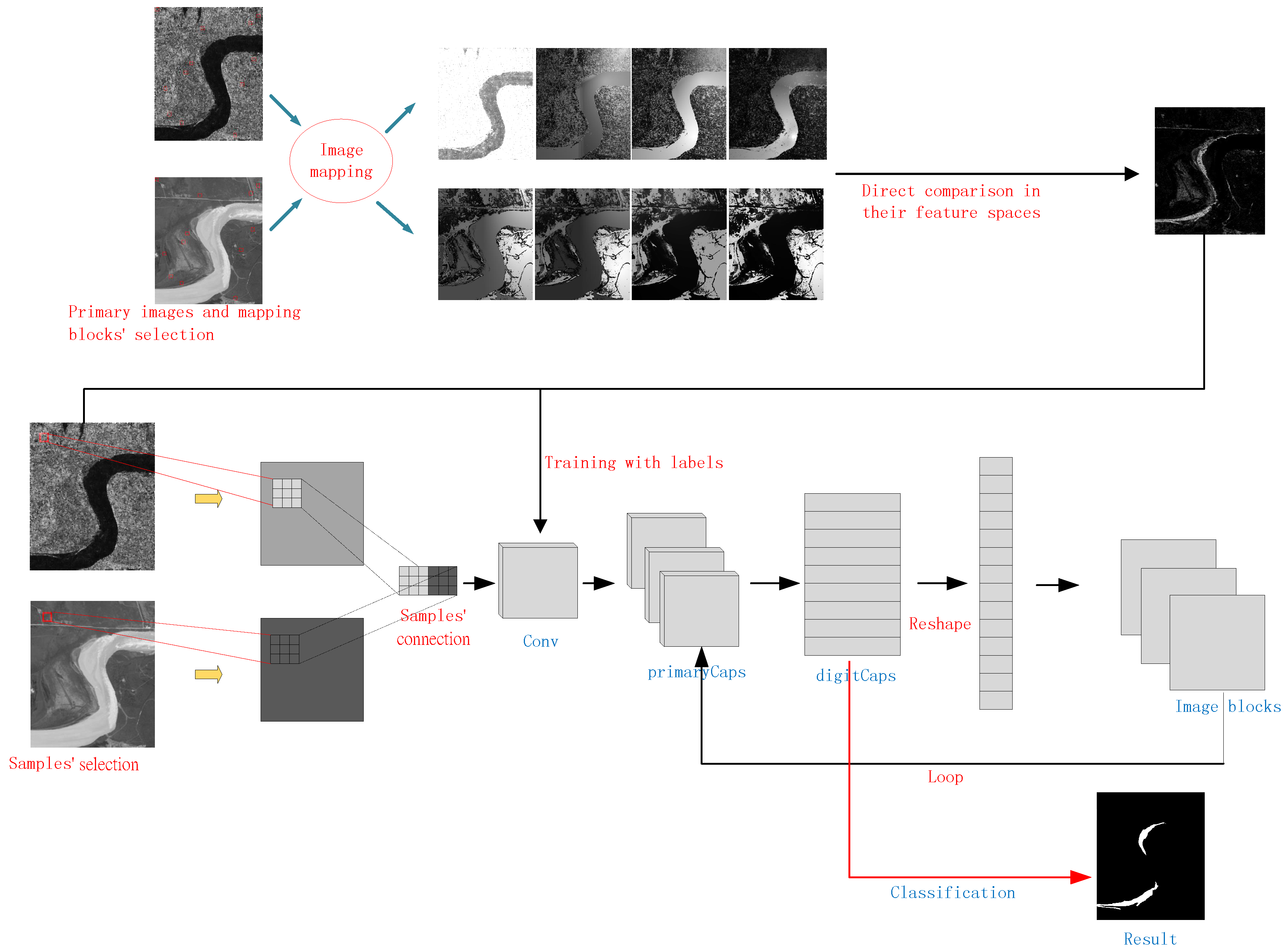
The entire flowchart of the proposed method is shown in Figure 1. After clustering by SOM, these two images are compared. Then, some rough unchanged regions are obtained. In these regions, some image blocks are selected randomly. The first step is to transform each pixel in the image according to the mapping method with these image blocks. Then, the SAR image is converted into the optical feature space pixel by pixel by the mapping method, and similarly, the optical image is converted into the SAR feature space. After that, these images are compared directly in two different feature spaces, respectively. Finally, the classification images, obtained by fusing these two difference maps, are used as the labels for training. Samples of the network are selected from the fused image, which is the black and white training labels. The selected samples are connected and input into the network. Finally a binary classification map is obtained.
3.2. SOM Clustering and Block Selection
In this paper, each pixel is considered to be the basic element in the image, and the proposed change detection method is performed at the pixel level. By clustering pixels, they can be divided into several heaps, and the pixels in the same heap have similar characteristics. SOM clustering is used mainly for selecting image blocks from the unchanged regions we detected. The input node is connected to the competing layer neurons by weights, and the neurons are connected to the adjacent neurons. The nodes of the input layer depend on the training samples, the input data. The number of nodes is equal to the number of the dimensions of the input data. The output layer is a topological structure composed of a group of neurons, the number of which is set to 100 (). SOM adjusts the weights of the network adaptively through the training samples, and the formula is as follows:
Here, i is the neuron index. The learning rate is a function of the training time t and the topological distance N, and the x is the training sample. is calculated according to the previous value . These parameters can be obtained by the method in [44]. The output layer in the trained network can not only determine the category of an input mode, but also reflect the approximate distribution of the input data. Thus, the input data can be clustered based on certain characteristics.
3.3. Image Mapping Method
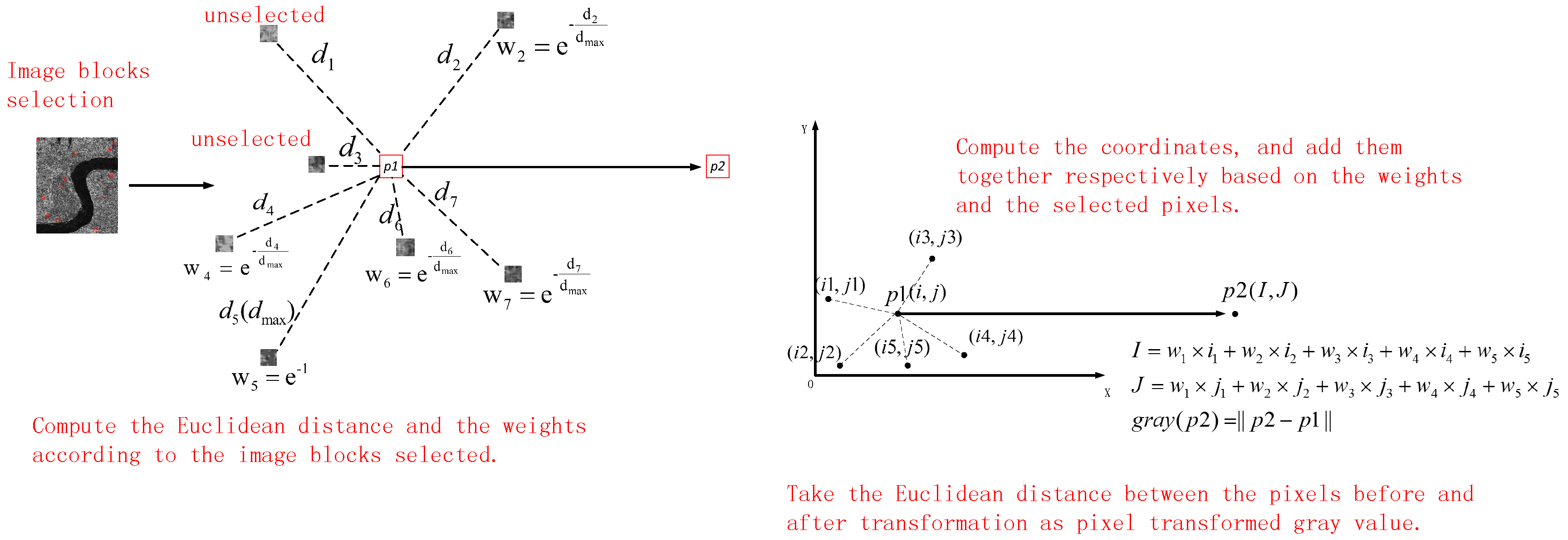
We can transform the images according to the obtained image blocks. There is a pair of heterogeneous images, the images before and after the event, representing Experimental Images 1 and 2, respectively. In heterogeneous images, some pixels have very close values in pre-event images, while their corresponding pixel gray values are more or less different in post-event images, even though they are not affected by the event. This is mainly caused by noise effects and differences in image mode. It is hard to compare them directly to detect changes. An image transformation from the original feature space to another is performed [45]. The image will be converted to a similar feature space as the post-event image for direct comparison.
The mapping method is shown in Figure 2. In this mapping method, the first step is that the k pixels are selected from the unchanged regions. These k pixels to be used for transformation are considered as potential values of the mapping pixel. The pixels that have the nearest gray value to the mapping pixel are used to estimate the missing attribute values, such as the pixel gray value in the optical feature space, according to the known attributes, such as the Euclidean distance and the pixel gray value in the SAR feature space. If a known attribute value is very close in one space, its missing portion should be close to the corresponding part of the mode also. Therefore, the nearest neighbors are found according to the known attribute, and the missing attribute will be filled by the weighted average of the k neighbor pixels. The strategy uses the weighted average of the k nearest similar pixel positions as the mapping expectation coordinates. Images 1 and 2 are represented in each other’s feature space respectively, such that their pixel gray values can be compared.
According to the Euclidean distance difference of the pixel position, k nearest pixel points [46,47] in the space are found, then the reliable neighbors are selected according to the pixel gray value difference. The pixel gray difference values are sorted for selection. The difference is obtained according to the corresponding position of Image 2. The weight value is obtained through the difference value. The following is the pixel mapping equation:
where k is the number of selected pixels used for transformation. The parameter is the k pixels’ value, and is the transformed value, which is viewed as the pixel gray value in another feature space. The weight is obtained by the equations below:
where is the ratio of two Euclidean distances. The numerator is the Euclidean distance between the pixel to be transformed and the selected pixel. The denominator is the max Euclidean distances between the k pixels and the pixel to be transformed.
The expected pixel gray value is obtained through the distance, and the Euclidean distance between them is the transformed pixel gray value.
Finally, we will integrate the difference images [48]. This is given by the equation below:
If based on one pixel only, it is likely to cause the wrong detection. However, if we make the opposite transformation, the pixels in Image 2 are associated with the feature space of Image 1. Some pixels in Image 2 that have close values may be closer to the pixels in Image 1. Thus, if the difference value is too large, the difference value will be more or less a little smaller. In this case, the sum of and will not be too large. This fusion process can utilize the information of the two feature spaces to suppress noise [49].
3.4. Sample Selection
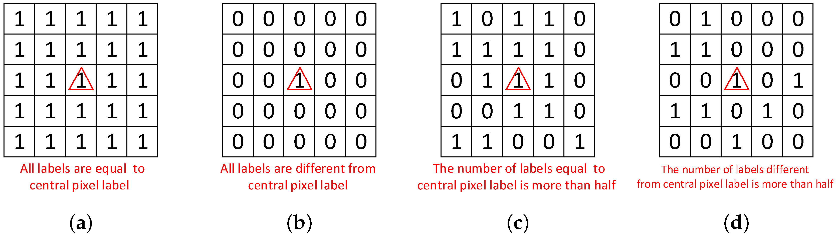
This section introduces how to select training samples to acquire reliable samples and a good trained network. The label map we obtained before contained correct labels and many false labels, namely unreliable ones. The higher the reliability of the selected training label is, the more correct the final result of the training will be. Suppose that the value of a training label in the label map is 1 and that this pixel has a neighborhood of , as shown in Figure 3.
Obviously, if the pixel gray values in this neighborhood are all 1, then the value of this label is reliable. Conversely, if other pixel gray values in this neighborhood are all 0, then the central pixel is considered a noise point. Therefore, the number of pixel labels in this neighborhood the same as central pixel can be used as a parameter for us to judge whether the sample is trustworthy or not. It can be judged according to the following formula:
where is the neighborhood and is the pixel in it. represents the pixel label. is the neighbor pixel label, and is the central pixel label. means the number of the pixel labels equal to the central pixel. n is the neighborhood size. Therefore, means the ratio of neighborhood pixels the same as the central label. Parameter should be set appropriately. If it is too large, the selected samples may be too few, which will have less diversity for training the network. However, if it is set too small, too many samples will be chosen. Many false labels will be selected, resulting in more wrong training results.
3.5. Deep Capsule Network and Parameter Settings
The deep capsule network is used to process the fused difference image obtained by the mapping method. Based on the reliable samples, we can finally obtain a well-trained network. The method of deepening the capsule network and the related parameter settings are shown in Figure 4. The deep capsule network for change detection can be accomplished by the following steps: (a) Select two samples and connect them directly into an size and use this as a network input. (b) Put the input into the Conv layer, using many convolution kernels to extract different simple feature information. The primarycaps layer further selects the extracted feature information and combines the feature information into vectors. The digitcaps layer normalizes these vectors and classifies them into a set of vectors. (c) Reshape these vectors into a one-dimensional vector, and reshape it as some image blocks of a certain size. Then, input them into the network as before. (d) Compute the norm of the vectors for classification and obtain the final classification results. Then, the parameters involved in the network are as marked in Figure 4.
The neurons in each layer are divided into groups, i.e., capsules. The output of the traditional neurons is increased and reshaped as a vector. It is rich in representing the features and the direction of the entity. The route consistency algorithm preserves the location information and other information of the entity. Network training is evaluated by using variance functions traditionally, while using the function below:
where c represents a type of classification and is a parameter. When c exists, is 1, else 0. , are the cases of missing the existing classification situations. is called the margin loss. There being a reconstruction process in the capsule network, we combine the margin loss and the reconstruction loss so as to make the training result more precise.
4. Experiment Study
The experiments mainly were performed based on two kinds of datasets. The first part in the experiments on performed on the homogeneous datasets and based on the deepened capsule network. The second part was performed on the heterogeneous datasets, and it was based on the proposed method.
4.1. Homogeneous Datasets
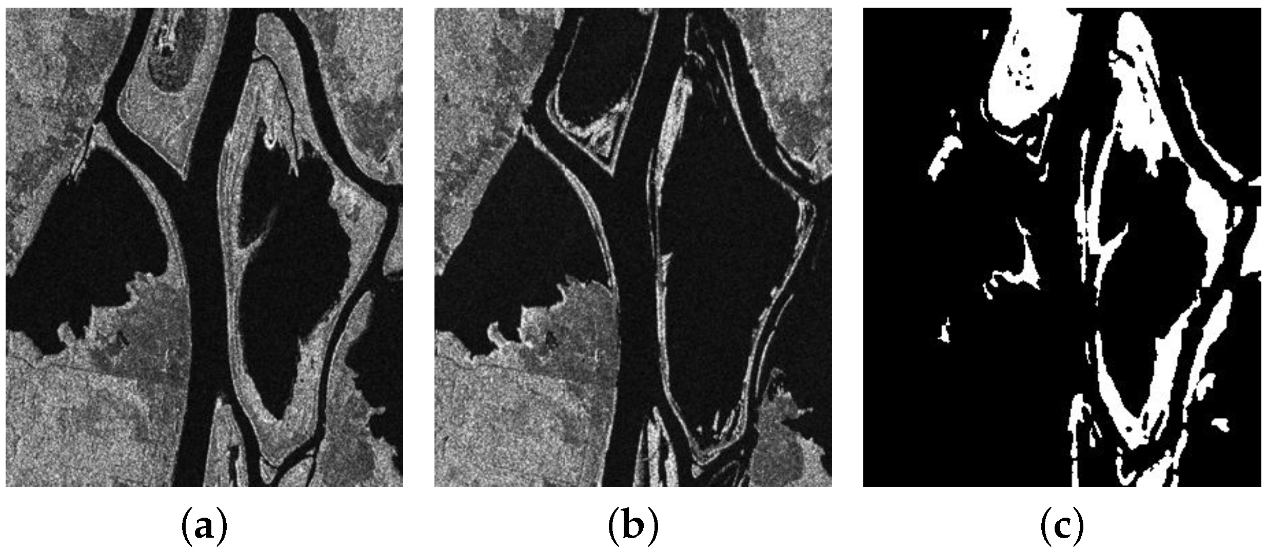
The first dataset consisted of two SAR images of the same size, , as shown in Figure 5a,b. These two images were obtained with Radarsat-2 in June 2008 and June 2009, respectively. They covered the same location of farmland along the Yellow River in Shandong Province, eastern China. The changed regions corresponded to the corrupted farmland, as shown in Figure 5c. The reference image served as the ground truth to indicate the actual changed regions. The reference image was acquired by integrating some prior information with image interpretation based on the original images and the actual situation.
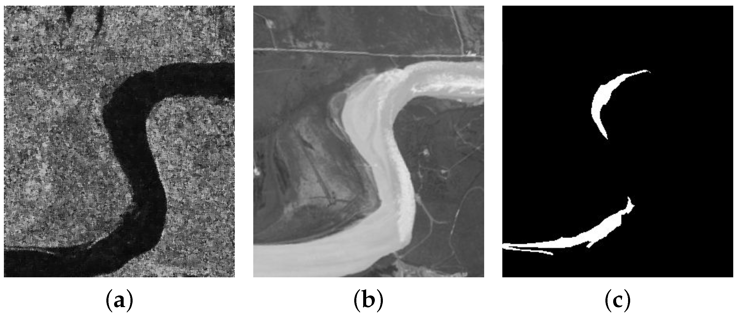
The Ottawa dataset was a group of two SAR images over the city of Ottawa acquired with Radarsat SAR sensors, and the size was pixels. The ground truth (reference image), which is shown in Figure 6c, was acquired by integrating some prior information of Figure 6a,b. The experiment on the Ottawa dataset was to evaluate water disaster. The white areas represent the changed areas, namely those areas affected.
4.2. Heterogeneous Datasets
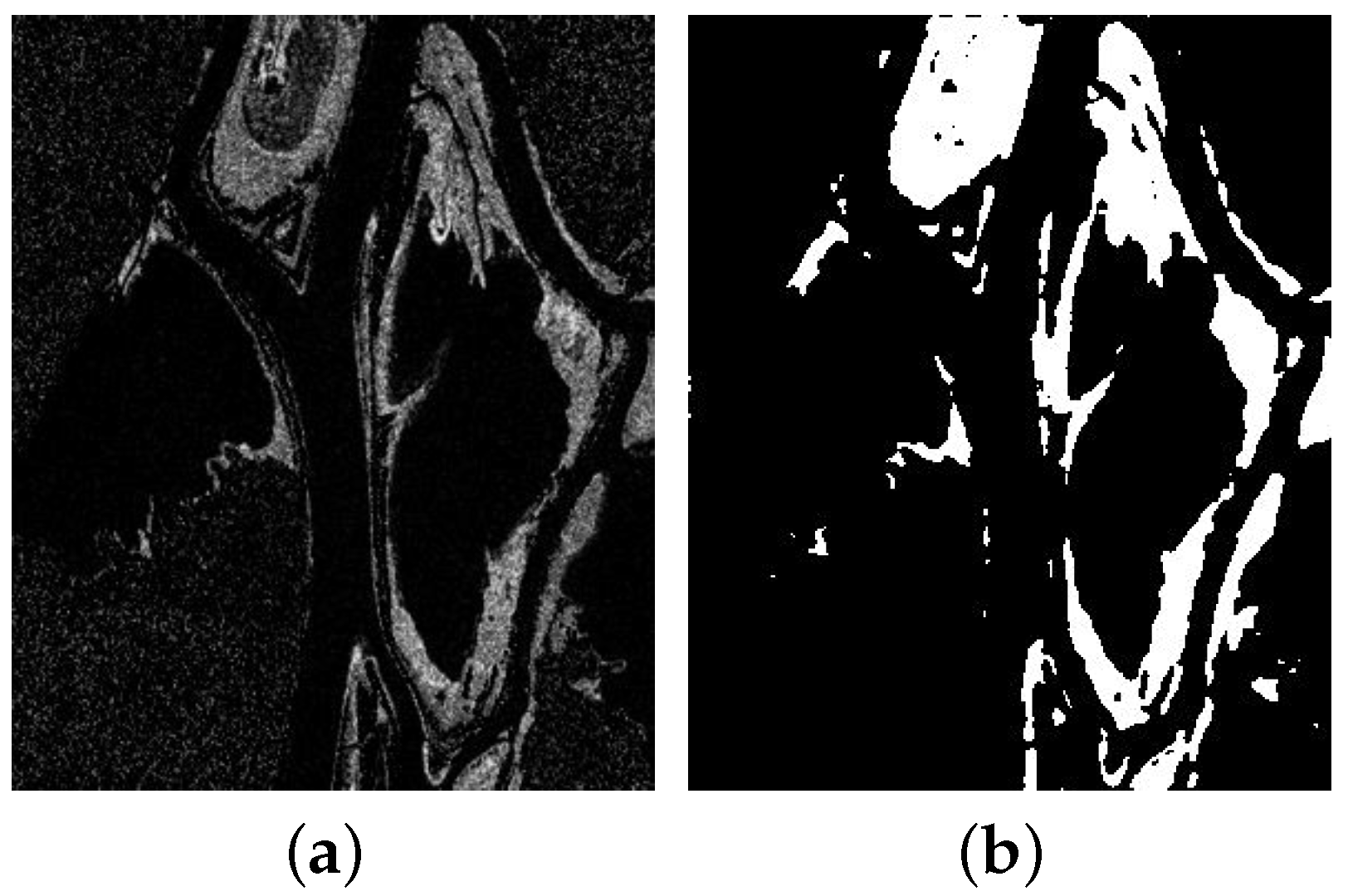
The third dataset consisted of a SAR image and an optical image with the same size of pixels, as shown in Figure 7a,b, respectively. The SAR image was also acquired with Radarsat-2 sensors from the Yellow River Estuary in June 2008. The optical image obtained in September 2010 was captured from Google Earth, covering the same region. These data provided by Google Earth integrated the imagery from both satellite and aerial photography. These satellite images were obtained from the Landsat-7 and QuickBird sensors. This dataset was used to study the change of the Yellow River affected by flood. Figure 7c is the reference image that reveals the actual changed regions.
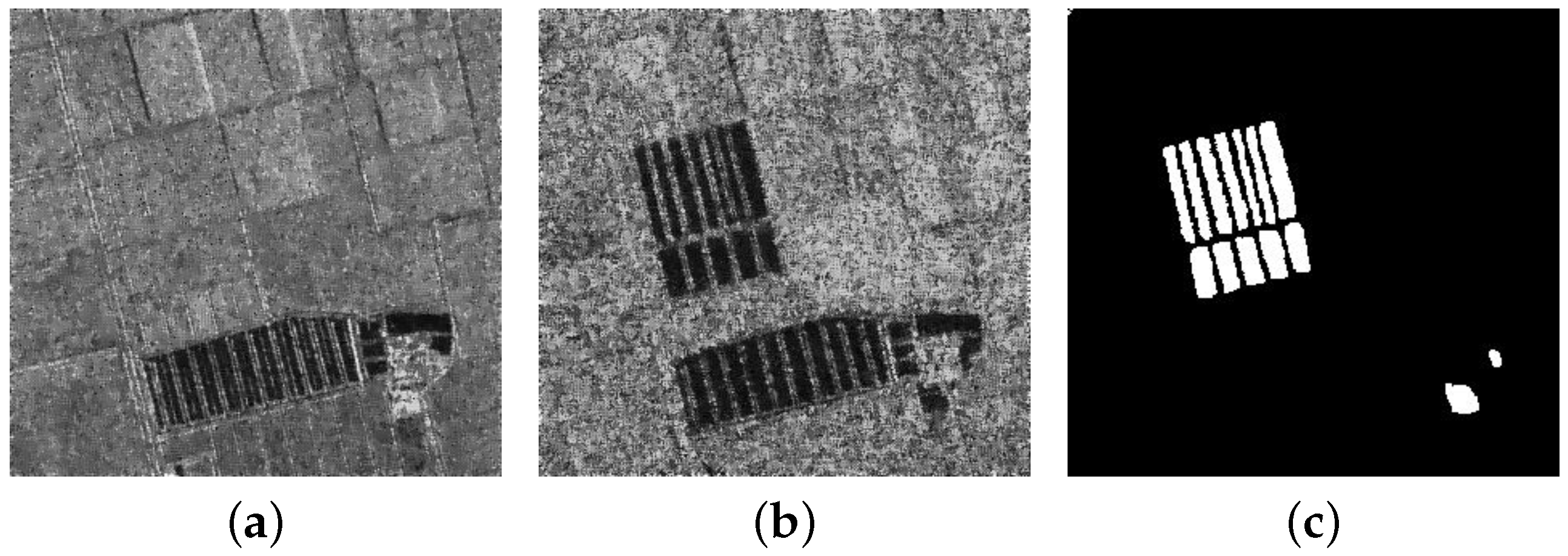
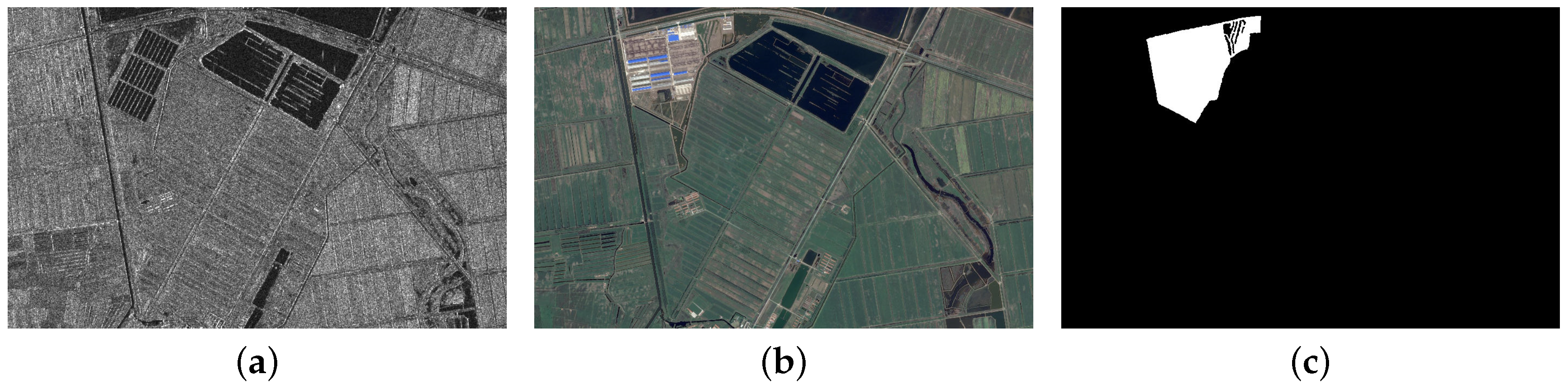
The last dataset contained a SAR image and an optical image, as shown in Figure 8a,b, respectively. This dataset covered a piece of the farmland area in Shuguang Village in Dongying City, China. The new buildings corresponding to the changed regions were built on the farmland, as shown in Figure 8c. The SAR and optical images were the same size, pixels. They were obtained in June 2008 and in September 2012, respectively.
4.3. Evaluation Criteria
The final classification results not only show the final change detection binary map, but also provide some evaluation criterion values to help with analyzing and observing the performance of the change detection results.
The parameters of the evaluation criteria are shown as follows: (1) the number of all pixels in the image N; (2) the actual number of changed pixels in the reference image and (3) the actual number of unchanged pixels in the reference image ; they both can be calculated with the reference image; (4) the number of changed pixels taken as unchanged pixels (false negative); and (5) the number of unchanged pixels taken as changed pixels (false positive). These two parameters can be calculated by comparing the reference image with the resulting image we obtained. We can calculate the overall error () as follows:
Another two parameters and , which have the opposite meaning of and , respectively, are calculated as follows:
where (true positive) means the amount of changed pixels correctly detected in both the reference image and the final experiment resulting image. (true negative) represents the number of unchanged pixels correctly detected in both the reference image and the resulting image.
For a further evaluation of the resulting image, we can calculate the percentage of correct classification () [50] as follows:
where shows the correct rate of the results. However, since the value N is usually large, the values obtained by different methods may be very similar in some situations. It is not enough to distinguish the quality of detection with only. Thus, we introduced the Kappa coefficient () [51] as another overall evaluation criterion. was used to evaluate the results. The higher the value is, the better the detection result is. The calculation method of is as follows:
where
depends on the sum of and . relies more on parameters containing more detailed classification information, so can further explain the quality of the change detection map.
4.4. Parameter Settings and Experiments on Homogeneous Datasets
4.4.1. Parameter Settings
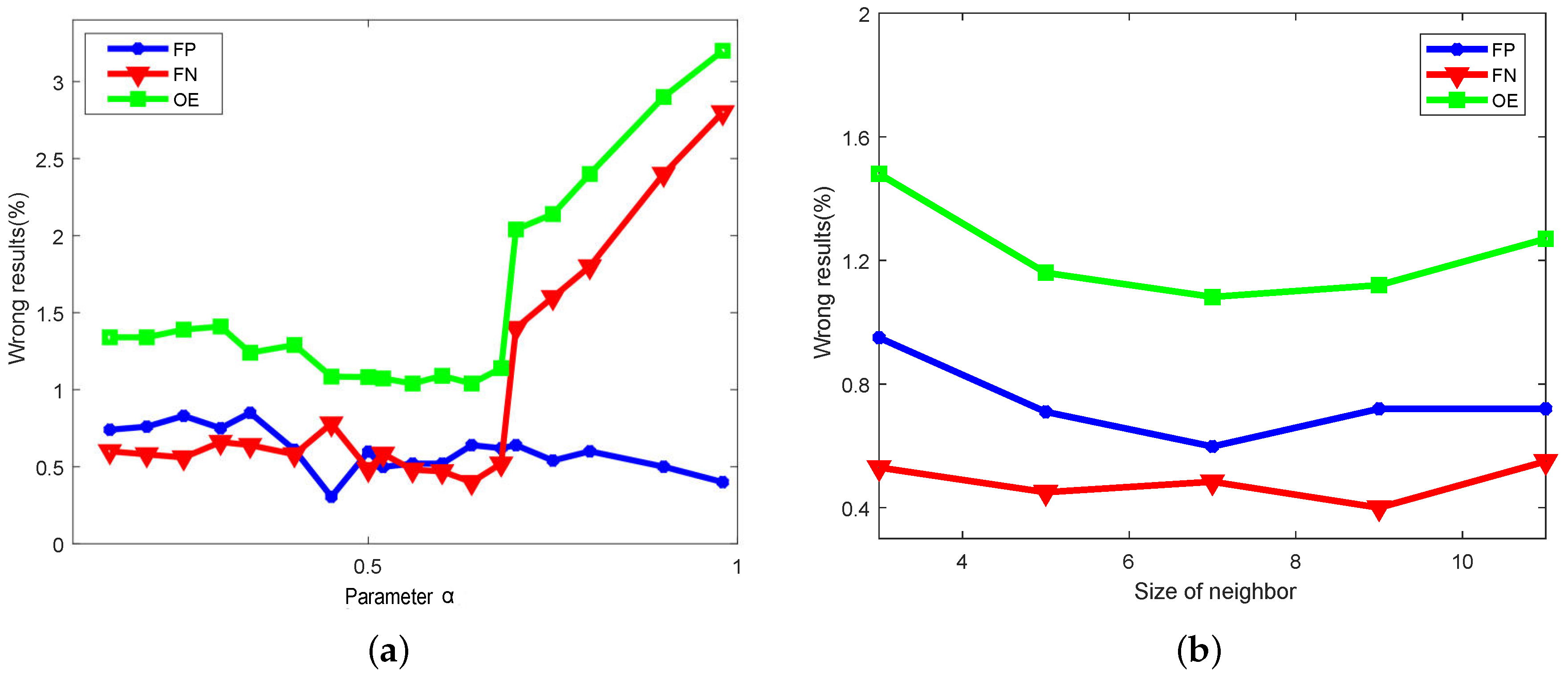
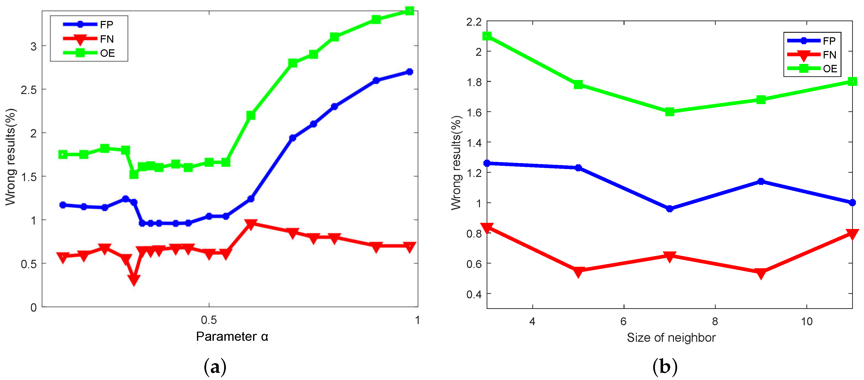
The relevant parameters should be set appropriately before evaluating the effectiveness of the proposed method. In the deep learning method, the structure of the whole network is very important. It is generally believed that more available features can be learned with more layers of the network. However, the complex structure of the network can also lead to extra calculation time. Therefore, the proper settings are very important. For change detection, the image scale is relatively small, and the structure does not need to be large. In such a process, 3 layers are sufficient for all parameter settings in the network. In fact, too few units in the hidden layer will affect the results, and too many units will bring many computational costs also. In the network, the window size n selected by the user and the sample selection parameter have important effects on the result. The value of n determines the amount of information we extract from the two original images. The value of the parameter determines the appropriate number of training samples. When n is too large, the classification of the central pixel is too affected by its neighbor pixels, and the calculation costs much more. In general, n is chosen to be in the vicinity of 5. It can be chosen from 3, 5, 7, 9, 11. Figure 9 shows the criteria of the parameters and the n size of neighbors, respectively. Lines of different colors represent different criteria on different datasets. The results show that was the best choice. When , the extracted information was not enough. On the contrary, when , the accuracy of the result was no better than . The reason may be that the local information extracts too much, so that the characteristics of the local pixels are covered. Figure 10 is the resulting map based on these parameters.
Overall, when , the performance was better than the others. In the following experiments, all datasets selected n as 7. Figure 11 depicts the effect of the parameters and n on the resulting image, respectively. Lines of different colors represent performance on different datasets. The results show that near was a good choice, so the following experiments were implemented according to . When n was too small, the sample reliability was not strong enough, and it was impossible to get good results through training. Conversely, when n was too large, the accuracy of the result was no better than . The reason is that the samples obtained contained only reliable ones, but the samples were not abundant enough and the sample size insufficient. is much better than others. In the following experiments, as was selected for all datasets. Figure 12 is the resulting map based on these parameters.
4.4.2. Experiments on Homogeneous Datasets
In the homogeneous image experiments, we compared the log-ratio (LR) method [52], the mean-ratio (MR) method [53], the SCCN method, and these methods based on the deep capsule network, D_LR, D_MR, and D_SCCN. The methods LR and MR are the most commonly-used homologous remote sensing image change detection methods and are simple and effective. The SCCN method is a heterogeneous change detection method, which is also suitable for change detection in homogeneous datasets.
In the experiment of the farmland dataset, the results obtained by the methods mentioned before are shown in Figure 13. The difference maps obtained by different methods were different. Based on the comparison between the resulting map and the reference image (ground truth), different evaluation criteria were obtained. They are listed in Table 1. It can be seen that the deep capsule network has improved results. In the experiment of the Ottawa dataset, several different difference maps and binary resulting images were obtained, which are shown in Figure 14. Comparing the resulting image with the reference map, we list the evaluation criteria of the results by the different methods in Table 2. Similarly, the deep capsule network had improved results. Both experiments showed the capacity of processing and improving the difference image.
4.5. Experiment Performance on Heterogeneous Datasets
In the next experiments, we will compare our methods (PROPOSED) with the change vector analysis (CVA) [54,55], ASDNN [56], SCCN, and PCCmethods. The CVA method is a very effective method for multi-spectrum change detection. The ASDNN method is a heterogeneous image change detection method based on the idea of SCCN. It is an improved method of SCCN and has a strong capability in heterogeneous image processing.
4.5.1. Experiment on the Yellow River Dataset
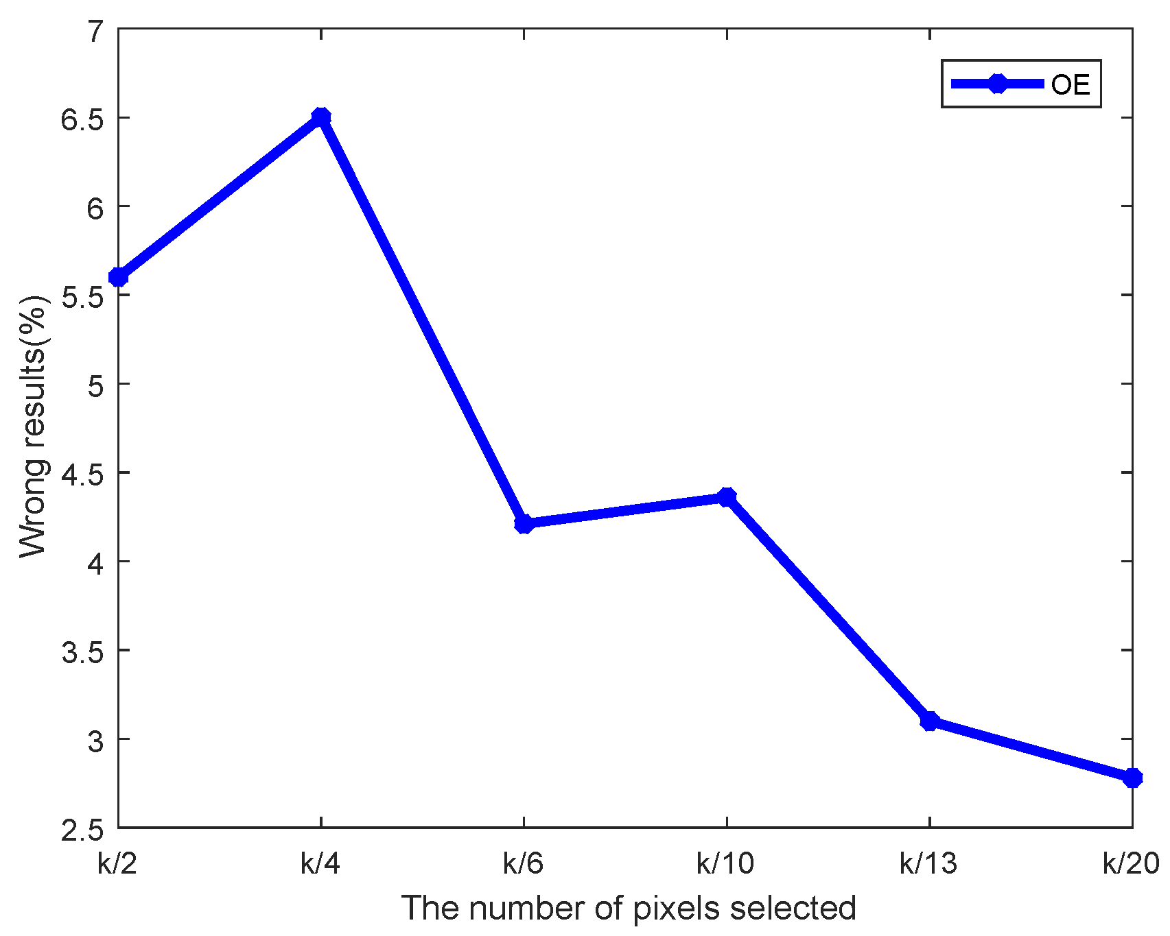
In the experiment of the Yellow River dataset, the image blocks were chosen randomly. When selected, they should be distributed as reasonably as possible. If just a certain block or part in the image is selected, the blocks cannot contain sufficient information, and it will not make the results more general, but accidental. In this experiment, k was selected as 1300, namely 13 small image blocks contained 100 pixels each. In Figure 15, six images are shown. These six images were the difference maps obtained by selecting different numbers of pixels from these image blocks. They were acquired based on these pixels. In Figure 16, in the results was obtained by the simple threshold segmentation method. It was suitable to select the number of pixels to be small in this dataset. When the number of selected pixels was , was the least. Other good results were based on this number being around 65.
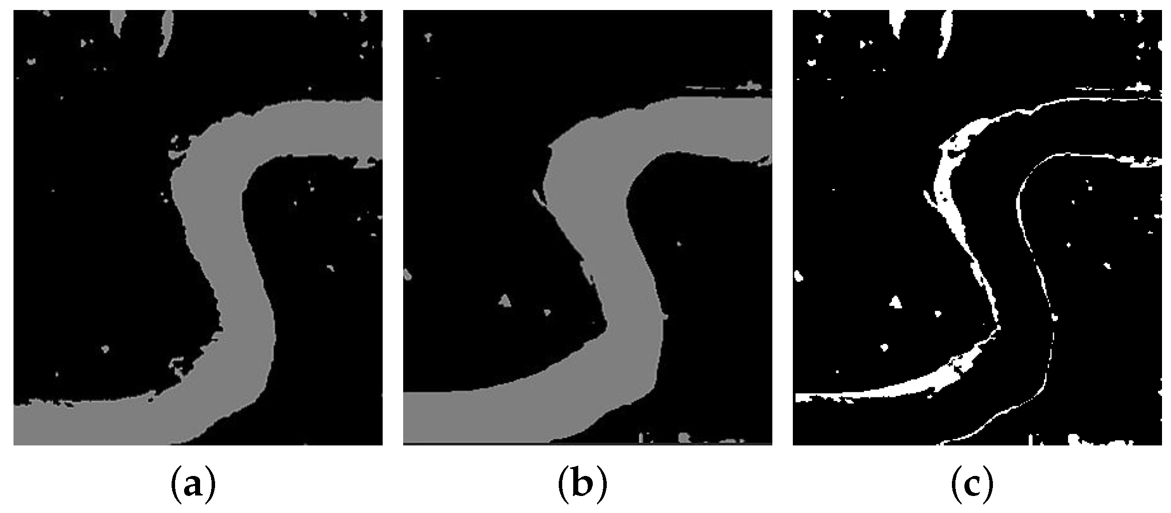
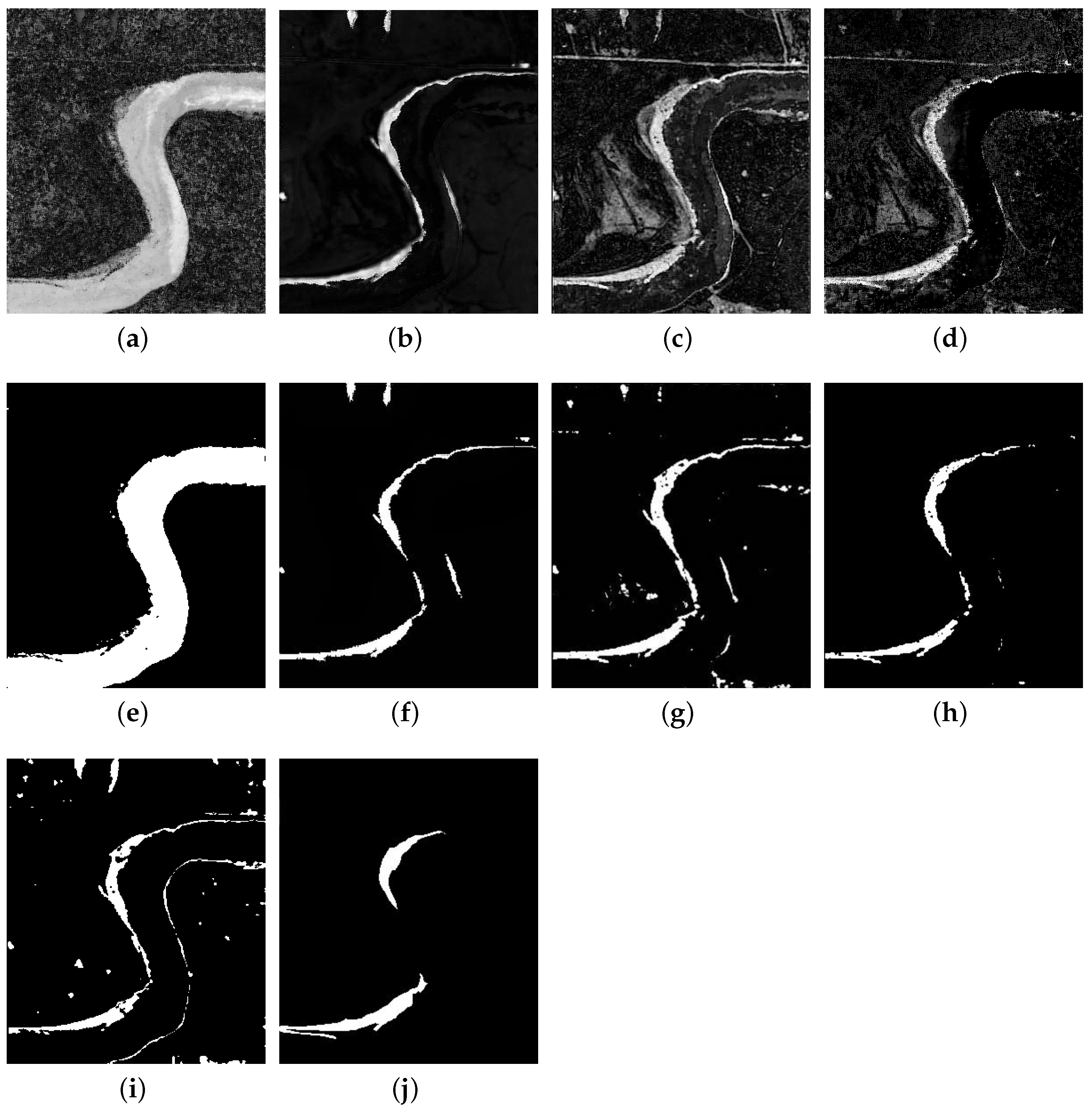
In this experiment, the PCC method was used to generate classifications, and the results are shown in Figure 17a,b. Each of these two images included two identifiable categories that represent land and rivers. The final binary resulting map can be obtained by direct comparison pixel by pixel, and it is shown in Figure 17c. Pixels with the same category of labels remained unchanged, and a different category of labels would be considered as changed. The difference images generated by the CVA, ASDNN, and SCCN methods and the corresponding resulting images are shown in Figure 18. Figure 18d,h shows the difference image and resulting map generated by our proposed method. The reference image is shown in Figure 18j.
It is shown that the quality of the difference image produced by our proposed method was significantly higher. It can be seen that the proposed method had the fewest false alarms. Table 3 shows the values of the evaluation criteria obtained by the five methods. The CVA method can utilize different spectrum information. However, it obtained the wrong change detection result because the spectra in this dataset had more gray information, but less color information. The accuracy of the proposed method achieved the best performance overall. PCC is a simple change detection approach, and its performance was affected by the classification algorithm while ignoring much detailed information. SCCN is an innovative method based on symmetric coupled deep convolutional neural networks. It exhibited a fairly high degree of accuracy in detecting changes in heterogeneous images, and its training samples were selected from regions that were unchanged. It blurred some locations belonging to the changed class. ASDNN performed better on this dataset. The performance of ASDNN was better in the main detection regions, and it can decrease many of the noises. However, our proposed method balanced these two problems. It can decrease as many of the noises as possible and detect the main regions in detail.
4.5.2. Experiment on Shuguang Village Dataset
In the Shuguang dataset experiment, image blocks were selected randomly. The same as above, they should be distributed as reasonably as possible when selected. In this experiment, k was selected as 4500, namely 15 small image blocks, each of which contained 300 pixels. There are six images shown in Figure 19. These pictures were based on different numbers of pixels selected from image blocks. Then simple difference maps were obtained. In Figure 20, the of the different results was obtained. When the number of selected pixels was , was the least. However, if the number was too small, such as 80, the result would be a little worse. A good choice for the number of pixels was about 200, as selected in this dataset. Fairly good mapping images could be obtained when the number was set around 200.
In this experiment, PCC method was used to generate classifications and resulting maps, as shown in Figure 21a,b. There were two identifiable types in the SAR image, namely farmland region and water region. In fact, there were also some buildings, but it was hard to identify these buildings using unsupervised classifiers. There were three identifiable categories in the optical image, namely farmland, water, and building regions. However, some farmland areas were not correctly classified. Therefore, such an error caused a change detection result, which was not good enough. The resulting map was obtained by direct comparison. The difference images generated by the proposed method, other methods, and the corresponding resulting images are shown in Figure 22.
According to Table 4, the proposed method obtained the best result among these methods. ASDNN and SCCN performed better than PCC. The evaluation criteria of proposed method were better than these two network methods. ASDNN was the best in the main region we wanted to detect. CVA also achieved a fairly good result. CVA can make full use of the color information in this kind of image, though it cannot detect the region of interest well. The same as the performance before, PCC detected nearly all of the regions that were to be detected, while containing too many unnecessary regions. The difference image obtained by the proposed method was better. In the SCCN method, most of the changed regions were detected, but some small detailed regions that were considered to be changed belonged to the unchanged regions in the reference map. The proposed method was superior to the other methods in terms of accuracy and detail.
5. Conclusions
In this paper, two heterogeneous images were transformed in the feature space at the pixel level and then compared in their respective feature spaces. Finally, the resulting classified images were sampled and input into the improved neural network to obtain the final classification result. The results obtained were better than those obtained by some current methods, but the drawback of the proposed method is that it was limited to SAR and certain optical images, rather than multi-spectral images, like high spectral images, natural images, etc. The future work is to explore the feasibility of this method on multi-spectral images, natural images, or other kinds of images.
Author Contributions
Investigation, W.M., Y.X., Y.W. and X.Z.; Supervision, Y.W. and L.J.; Writing—original draft, W.M. and Y.X.; Writing—review and editing, W.M. and H.Y.
Funding
The research was jointly supported by the National Natural Science Foundations of China (No. 61702392, 61671350, 61772400), and the China Postdoctoral Science Foundation (No. 2018T111022, 2017M623127).
Acknowledgments
Thanks to the help of the advices of editors, We are able to complete this paper successfully.
Conflicts of Interest
The authors declare no conflict of interest.
References
- Brunner, D.; Lemoine, G.; Bruzzone, L. Earthquake damage assessment of buildings using VHR optical and SAR imagery. IEEE Trans. Geosci. Remote Sens. 2010, 48, 2403–2420. [Google Scholar] [CrossRef]
- Lv, Z.; Liu, T.; Wan, Y.; Benediktsson, J.A.; Zhang, X. Post-Processing Approach for Refining Raw Land Cover Change Detection of Very High-Resolution Remote Sensing Images. Remote Sens. 2018, 10, 472. [Google Scholar] [CrossRef]
- Mai, D.S.; Long, T.N. Semi-Supervised Fuzzy C-Means Clustering for Change Detection from Multispectral Satellite Image. In Proceedings of the 2015 IEEE International Conference on Fuzzy Systems, Istanbul, Turkey, 2–5 August 2015. [Google Scholar]
- Nielsen, A.A. The regularized iteratively reweighted MAD method for change detection in multi-and hyperspectral data. IEEE Trans. Image Process. 2007, 16, 463–478. [Google Scholar] [CrossRef] [PubMed]
- Gong, M.; Cao, Y.; Wu, Q. A neighborhood-based ratio approach for change detection in SAR images. IEEE Geosci. Remote Sens. Lett. 2012, 9, 307–311. [Google Scholar] [CrossRef]
- Conradsen, K.; Nielsen, A.A.; Schou, J.; Skriver, H. A test statistic in the complex Wishart distribution and its application to change detection in polarimetric SAR data. IEEE Trans. Geosci. Remote Sens. 2003, 41, 4–19. [Google Scholar] [CrossRef]
- Singh, A. Review Article Digital change detection techniques using remotely-sensed data. Int. J. Remote Sens. 1989, 10, 989–1003. [Google Scholar] [CrossRef] [Green Version]
- Li, Y.; Wang, X.; Zhan, Z.; Wang, Y. A Novel Approach to Unsupervised Change Detection Based on Hybrid Spectral Difference. Remote Sens. 2018, 10, 841. [Google Scholar]
- Liu, W.; Jie, Y.; Zhao, J.; Le, Y. A Novel Method of Unsupervised Change Detection Using Multi-Temporal PolSAR Images. Remote Sens. 2017, 9, 1135. [Google Scholar] [CrossRef]
- Ma, W.; Wu, Y.; Gong, M.; Xiong, Y.; Yang, H.; Hu, T. Change detection in SAR images based on matrix factorisation and a Bayes classifier. Int. J. Remote Sens. 2018, 40, 1–26. [Google Scholar] [CrossRef]
- Kit, O.; Lüdeke, M. Automated detection of slum area change in Hyderabad, India using multitemporal satellite imagery. ISPRS J. Photogramm. Remote Sens. 2013, 83, 130–137. [Google Scholar] [CrossRef] [Green Version]
- Marchesi, S.; Bovolo, F.; Bruzzone, L. A context-sensitive technique robust to registration noise for change detection in VHR multispectral images. IEEE Trans. Image Process. 2010, 19, 1877–1889. [Google Scholar] [CrossRef] [PubMed]
- Kuruoglu, E.E.; Zerubia, J. Modeling SAR images with a generalization of the Rayleigh distribution. IEEE Trans. Image Process. 2004, 13, 527–533. [Google Scholar] [CrossRef] [PubMed]
- Dawn, S.; Saxena, V.; Sharma, B. Remote sensing image registration techniques: A survey. In Proceedings of the 2010 International Conference on Image and Signal Processing, Quebec, QC, Canada, 30 June–2 July 2010; pp. 103–112. [Google Scholar]
- Lu, D.; Mausel, P.; Brondizio, E.; Moran, E. Change detection techniques. Int. J. Remote Sens. 2004, 25, 2365–2401. [Google Scholar] [CrossRef]
- Prendes, J.; Chabert, M.; Pascal, F.; Giros, A.; Tourneret, J.Y. A new multivariate statistical model for change detection in images acquired by homogeneous and heterogeneous sensors. IEEE Trans. Image Process. 2015, 24, 799–812. [Google Scholar] [CrossRef] [PubMed]
- Meng, L.; Hong, Z.; Chao, W.; Fan, W. Change Detection of Multilook Polarimetric SAR Images Using Heterogeneous Clutter Models. IEEE Trans. Geosci. Remote Sens. 2014, 52, 7483–7494. [Google Scholar] [CrossRef]
- Hou, B.; Wei, Q.; Zheng, Y.; Wang, S. Unsupervised change detection in SAR image based on Gauss-log ratio image fusion and compressed projection. IEEE J. Sel. Top. Appl. Earth Obs. Remote Sens. 2014, 7, 3297–3317. [Google Scholar] [CrossRef]
- Bovolo, F.; Bruzzone, L. A detail-preserving scale-driven approach to change detection in multitemporal SAR images. IEEE Trans. Geosci. Remote Sens. 2005, 43, 2963–2972. [Google Scholar] [CrossRef] [Green Version]
- Zheng, Y.; Zhang, X.; Hou, B.; Liu, G. Using Combined Difference Image and k-Means Clustering for SAR Image Change Detection. IEEE Geosci. Remote Sens. Lett. 2014, 11, 691–695. [Google Scholar] [CrossRef]
- Kittler, J.; Illingworth, J. Minimum error thresholding. Pattern Recognit. 1986, 19, 41–47. [Google Scholar] [CrossRef]
- Otsu, N. A threshold selection method from gray-level histograms. IEEE Trans. Syst. Man Cybern. 1979, 9, 62–66. [Google Scholar] [CrossRef]
- Celik, T. Unsupervised change detection in satellite images using principal component analysis and k-means clustering. IEEE Geosci. Remote Sens. Lett. 2009, 6, 772–776. [Google Scholar] [CrossRef]
- Yetgin, Z. Unsupervised Change Detection of Satellite Images Using Local Gradual Descent. IEEE Trans. Geosci. Remote Sens. 2012, 50, 1919–1929. [Google Scholar] [CrossRef]
- Krizhevsky, A.; Sutskever, I.; Hinton, G.E. Imagenet classification with deep convolutional neural networks. In Advances in Neural Information Processing Systems; MIT Press: Cambridge, MA, USA, 2012; pp. 1097–1105. [Google Scholar]
- Sermanet, P.; Chintala, S.; LeCun, Y. Convolutional neural networks applied to house numbers digit classification. In Proceedings of the IEEE 2012 21st International Conference on Pattern Recognition (ICPR), Tsukuba, Japan, 11–15 November 2012; pp. 3288–3291. [Google Scholar]
- Gong, M.; Niu, X.; Zhang, P.; Li, Z. Generative Adversarial Networks for Change Detection in Multispectral Imagery. IEEE Geosci. Remote Sens. Lett. 2017, 14, 2310–2314. [Google Scholar] [CrossRef]
- Gong, M.; Zhao, J.; Liu, J.; Miao, Q.; Jiao, L. Change detection in synthetic aperture radar images based on deep neural networks. IEEE Trans. Neural Netw. Learn. Syst. 2016, 27, 125–138. [Google Scholar] [CrossRef] [PubMed]
- Le Roux, N.; Bengio, Y. Representational power of restricted Boltzmann machines and deep belief networks. Neural Comput. 2008, 20, 1631–1649. [Google Scholar] [CrossRef] [PubMed]
- Mubea, K.; Menz, G. Monitoring land-use change in Nakuru (Kenya) using multi-sensor satellite data. Adv. Remote Sens. 2012, 1, 74. [Google Scholar] [CrossRef]
- Jensen, J.; Ramsey, E.; Mackey, H., Jr.; Sharitz, R.; Christensen, E. Inland wetland change detection using aircraft MSS (multispectral scanner) data. Photogramm. Eng. Remote Sens. 1987, 53, 521–529. [Google Scholar]
- Gong, M.; Zhang, P.; Su, L.; Liu, J. Coupled dictionary learning for change detection from multisource data. IEEE Trans. Geosci. Remote Sens. 2016, 54, 7077–7091. [Google Scholar] [CrossRef]
- Gens, R.; Domingos, P.M. Deep symmetry networks. In Advances in Neural Information Processing Systems; MIT Press: Cambridge, MA, USA, 2014; pp. 2537–2545. [Google Scholar]
- Kohonen, T. Self-organized formation of topologically correct feature maps. Biol. Cybern. 1982, 43, 59–69. [Google Scholar] [CrossRef]
- Ke, W.; Qian, D.; Yi, W.; Yang, Y. Supervised Sub-Pixel Mapping for Change Detection from Remotely Sensed Images with Different Resolutions. Remote Sens. 2017, 9, 284. [Google Scholar] [Green Version]
- Vesanto, J.; Alhoniemi, E. Clustering of the self-organizing map. IEEE Trans. Neural Netw. 2000, 11, 586–600. [Google Scholar] [CrossRef] [PubMed] [Green Version]
- Sabour, S.; Frosst, N.; Hinton, G.E. Dynamic routing between capsules. In Advances in Neural Information Processing Systems; MIT Press: Cambridge, MA, USA, 2017; pp. 3856–3866. [Google Scholar]
- Cohen, T.; Welling, M. Group equivariant convolutional networks. In Proceedings of the 2016 International Conference on Machine Learning, New York, NY, USA, 19–24 June 2016; pp. 2990–2999. [Google Scholar]
- Mhaskar, H.N.; Poggio, T. Deep vs. shallow networks: An approximation theory perspective. Anal. Appl. 2016, 14, 829–848. [Google Scholar] [CrossRef] [Green Version]
- Wu, F.; Yang, X.H.; Packard, A.; Becker, G. Induced L2-norm control for LPV systems with bounded parameter variation rates. Int. J. Robust Nonlinear Control 1996, 6, 983–998. [Google Scholar] [CrossRef] [Green Version]
- Wang, D.; Liu, Q. An Optimization View on Dynamic Routing Between Capsules. In Proceedings of the 6th International Conference on Learning Representations, Vancouver, BC, Canada, 30 April–3 May 2018. [Google Scholar]
- Olshausen, B.A.; Anderson, C.H.; Van Essen, D.C. A neurobiological model of visual attention and invariant pattern recognition based on dynamic routing of information. J. Neurosci. 1993, 13, 4700–4719. [Google Scholar] [CrossRef] [PubMed]
- Jaiswal, A.; AbdAlmageed, W.; Natarajan, P. CapsuleGAN: Generative Adversarial Capsule Network. arXiv, 2018; arXiv:1802.06167. [Google Scholar]
- Santos, M.D.; Shiguemori, E.H.; Mota, R.L.; Ramos, A.C. Change detection in satellite images using self-organizing maps. In Proceedings of the IEEE 2015 12th International Conference on Information Technology-New Generations (ITNG), Las Vegas, NV, USA, 13–15 April 2015; pp. 662–667. [Google Scholar]
- Lyu, H.; Lu, H.; Mou, L. Learning a Transferable Change Rule from a Recurrent Neural Network for Land Cover Change Detection. Remote Sens. 2016, 8, 506. [Google Scholar] [CrossRef]
- Liu, Z.G.; Pan, Q.; Dezert, J.; Martin, A. Adaptive imputation of missing values for incomplete pattern classification. Pattern Recognit. 2016, 52, 85–95. [Google Scholar] [CrossRef] [Green Version]
- García-Laencina, P.J.; Sancho-Gómez, J.L.; Figueiras-Vidal, A.R. Pattern classification with missing data: A review. Neural Comput. Appl. 2010, 19, 263–282. [Google Scholar] [CrossRef]
- Gong, M.; Zhou, Z.; Ma, J. Change detection in synthetic aperture radar images based on image fusion and fuzzy clustering. IEEE Trans. Image Process. 2012, 21, 2141–2151. [Google Scholar] [CrossRef] [PubMed]
- Hussain, M.; Chen, D.; Cheng, A.; Wei, H.; Stanley, D. Change detection from remotely sensed images: From pixel-based to object-based approaches. ISPRS J. Photogramm. Remote Sens. 2013, 80, 91–106. [Google Scholar] [CrossRef]
- Rosin, P.L.; Ioannidis, E. Evaluation of global image thresholding for change detection. Pattern Recognit. Lett. 2003, 24, 2345–2356. [Google Scholar] [CrossRef] [Green Version]
- Brennan, R.L.; Prediger, D.J. Coefficient kappa: Some uses, misuses, and alternatives. Educ. Psychol. Meas. 1981, 41, 687–699. [Google Scholar] [CrossRef]
- Bujor, F.; Trouvé, E.; Valet, L.; Nicolas, J.M.; Rudant, J.P. Application of log-cumulants to the detection of spatiotemporal discontinuities in multitemporal SAR images. IEEE Trans. Geosci. Remote Sens. 2004, 42, 2073–2084. [Google Scholar] [CrossRef]
- Inglada, J.; Mercier, G. A New Statistical Similarity Measure for Change Detection in Multitemporal SAR Images and Its Extension to Multiscale Change Analysis. IEEE Trans. Geosci. Remote Sens. 2011, 45, 1432–1445. [Google Scholar] [CrossRef]
- Lambin, E.F.; Strahlers, A.H. Change-vector analysis in multitemporal space: A tool to detect and categorize land-cover change processes using high temporal-resolution satellite data. Remote Sens. Environ. 1994, 48, 231–244. [Google Scholar] [CrossRef]
- Johnson, R.D.; Kasischke, E. Change vector analysis: A technique for the multispectral monitoring of land cover and condition. Int. J. Remote Sens. 1998, 19, 411–426. [Google Scholar] [CrossRef]
- Zhao, W.; Wang, Z.; Gong, M.; Liu, J. Discriminative Feature Learning for Unsupervised Change Detection in Heterogeneous Images Based on a Coupled Neural Network. IEEE Trans. Geosci. Remote Sens. 2017, 55, 7066–7080. [Google Scholar] [CrossRef]
Figure 1.
Flowchart of the proposed method for remote sensing image change detection.

Figure 2.
The process of image mapping.

Figure 3.
Different label neighbor information and sample selection according to the threshold. (a) All the labels are the same as the central pixel label. (b) All the labels are different from the central pixel label. (c) More than half of the labels are the same as the central pixel. (d) More than half of the labels are different from the central pixel.

Figure 4.
The flowchart of the capsule network deepened in a certain way.

Figure 5.
Farmland dataset. (a) SAR image acquired in 2008. (b) Optical image acquired in 2009. (c) Reference image.
Figure 5.
Farmland dataset. (a) SAR image acquired in 2008. (b) Optical image acquired in 2009. (c) Reference image.

Figure 6.
Ottawa dataset. (a) SAR image acquired in 2008. (b) Optical image acquired in 2010. (c) Reference image.
Figure 6.
Ottawa dataset. (a) SAR image acquired in 2008. (b) Optical image acquired in 2010. (c) Reference image.

Figure 7.
Yellow River dataset. (a) SAR image acquired in May 1997. (b) Optical image acquired in August 1997. (c) Reference image.
Figure 7.
Yellow River dataset. (a) SAR image acquired in May 1997. (b) Optical image acquired in August 1997. (c) Reference image.

Figure 8.
Shuguang Village dataset. (a) SAR image acquired in 2008. (b) Optical image acquired in 2012. (c) Reference image.
Figure 8.
Shuguang Village dataset. (a) SAR image acquired in 2008. (b) Optical image acquired in 2012. (c) Reference image.

Figure 9.
(a) Relationship between the size of the neighbor and , , and on the farmland dataset. (b) Relationship between the parameter and the criteria on the farmland dataset.
Figure 9.
(a) Relationship between the size of the neighbor and , , and on the farmland dataset. (b) Relationship between the parameter and the criteria on the farmland dataset.

Figure 10.
(a) Difference map of the farmland dataset. (b) Resulting map by the deep capsule network.
Figure 10.
(a) Difference map of the farmland dataset. (b) Resulting map by the deep capsule network.

Figure 11.
(a) Relationship between the size of the neighbor and , , and on the Ottawa dataset. (b) Relationship between the parameter and the criteria on the Ottawa dataset.
Figure 11.
(a) Relationship between the size of the neighbor and , , and on the Ottawa dataset. (b) Relationship between the parameter and the criteria on the Ottawa dataset.

Figure 12.
(a) Difference map of the Ottawa dataset. (b) Resulting map by the deep capsule network.

Figure 13.
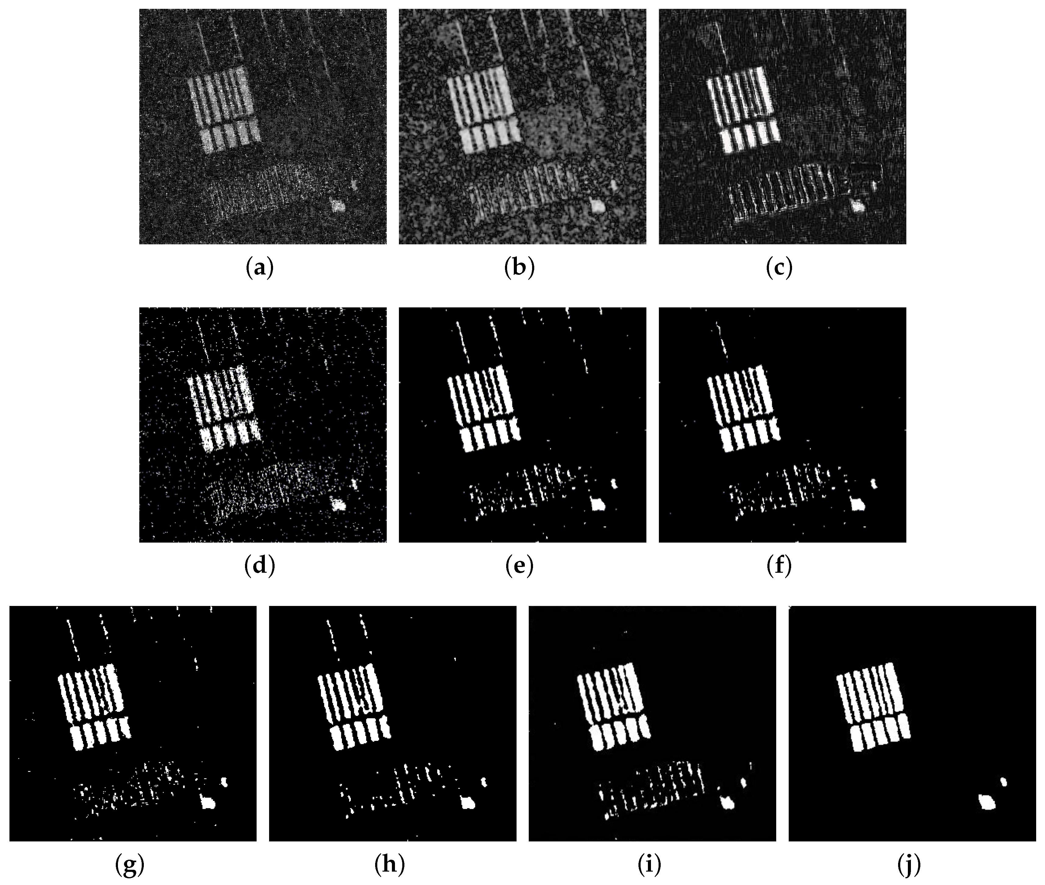
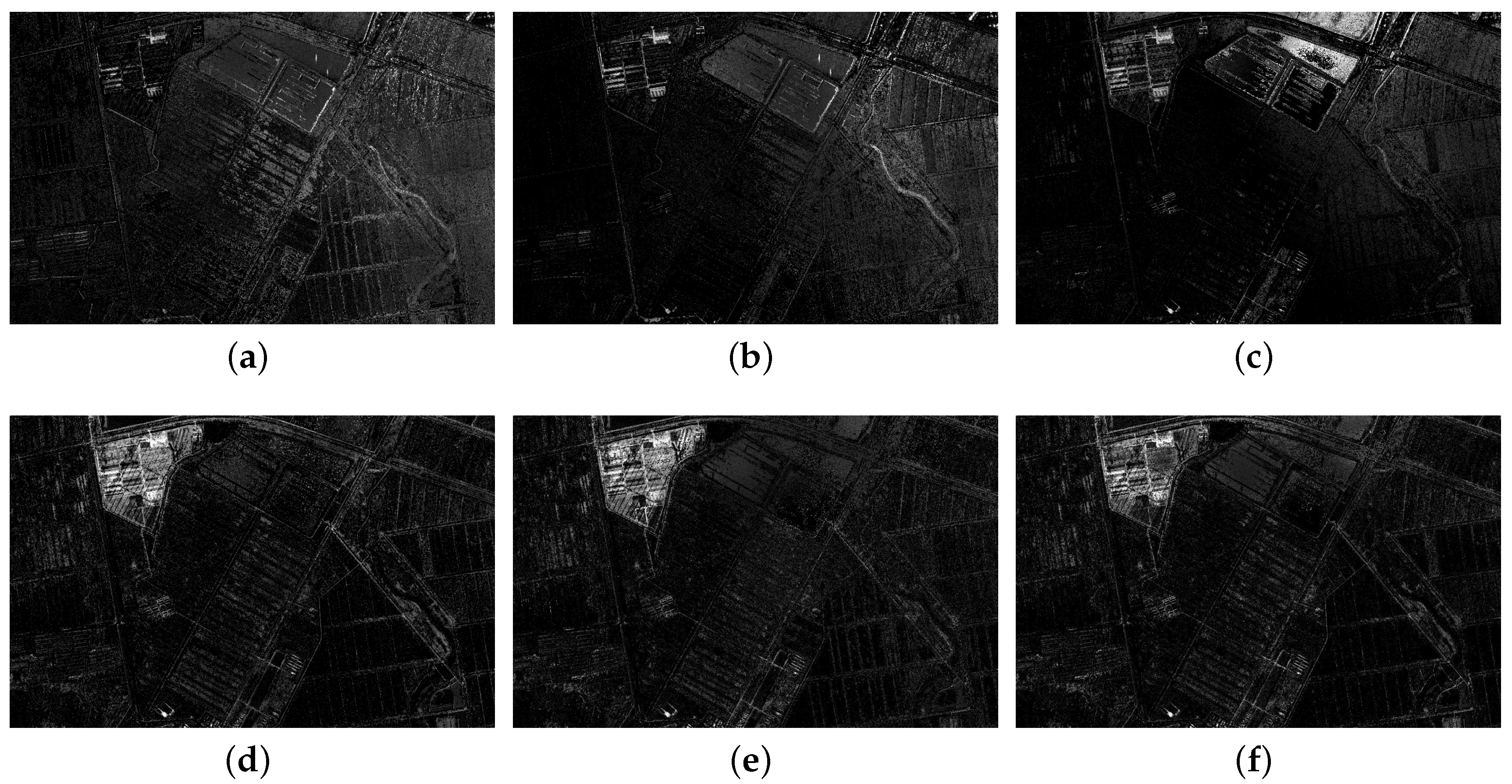
Difference maps and resulting maps of the farmland dataset obtained by different methods. (a) Difference map by the log-ratio (LR). (b) Difference map by the mean-ratio (MR). (c) Difference map by SCCN. (d) Resulting map by LR. (e) Resulting map by MR. (f) Resulting map by SCCN. (g) Resulting map by DCAPSbased on LR (D_LR). (h) Resulting map by DCAPS based on MR (D_MR). (i) Resulting map by DCAPS based on SCCN (D_SCCN) (j) Reference map.
Figure 13.
Difference maps and resulting maps of the farmland dataset obtained by different methods. (a) Difference map by the log-ratio (LR). (b) Difference map by the mean-ratio (MR). (c) Difference map by SCCN. (d) Resulting map by LR. (e) Resulting map by MR. (f) Resulting map by SCCN. (g) Resulting map by DCAPSbased on LR (D_LR). (h) Resulting map by DCAPS based on MR (D_MR). (i) Resulting map by DCAPS based on SCCN (D_SCCN) (j) Reference map.

Figure 14.
Difference maps and resulting maps of the Ottawa dataset obtained by different methods. (a) Difference map by LR. (b) Difference map by MR. (c) Difference map by SCCN. (d) Resulting map by LR. (e) Resulting map by MR. (f) Resulting map by SCCN. (g) Resulting map by DCAPS based on LR (D_LR). (h) Resulting map by DCAPS based on MR (D_MR). (i) Resulting map by DCAPS based on SCCN (D_SCCN) (j) Reference map.

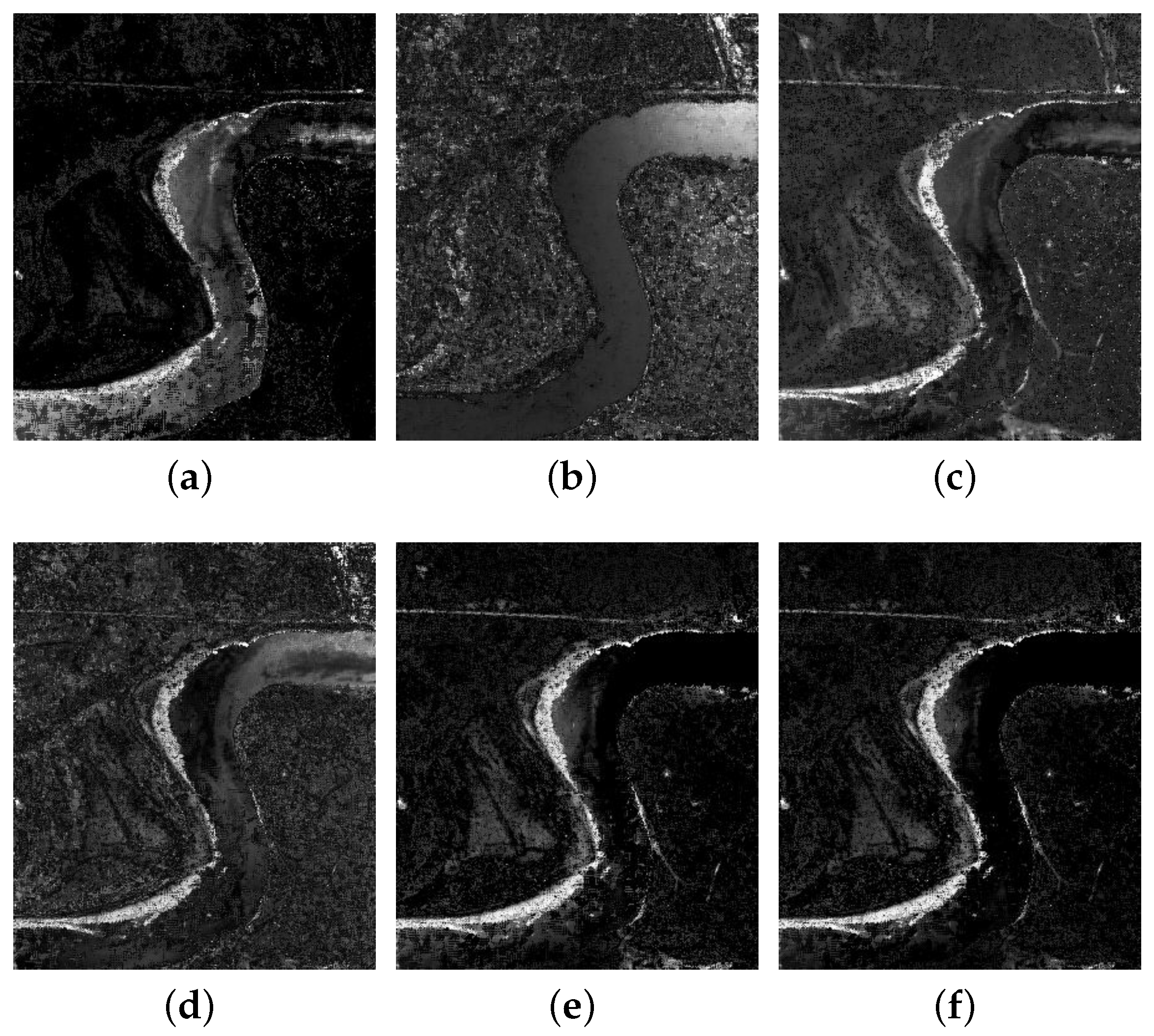
Figure 15.
The difference images for the Yellow River dataset obtained according to different numbers of selected pixels. (a) Difference image when the number is . (b) Difference image when the number is . (c) Difference image when the number is . (d) Difference image when the number is . (e) Difference image when the number is . (f) Difference image when the number is .

Figure 16.
The overall error () on the Yellow River dataset according to different numbers of pixels selected.
Figure 16.
The overall error () on the Yellow River dataset according to different numbers of pixels selected.

Figure 17.
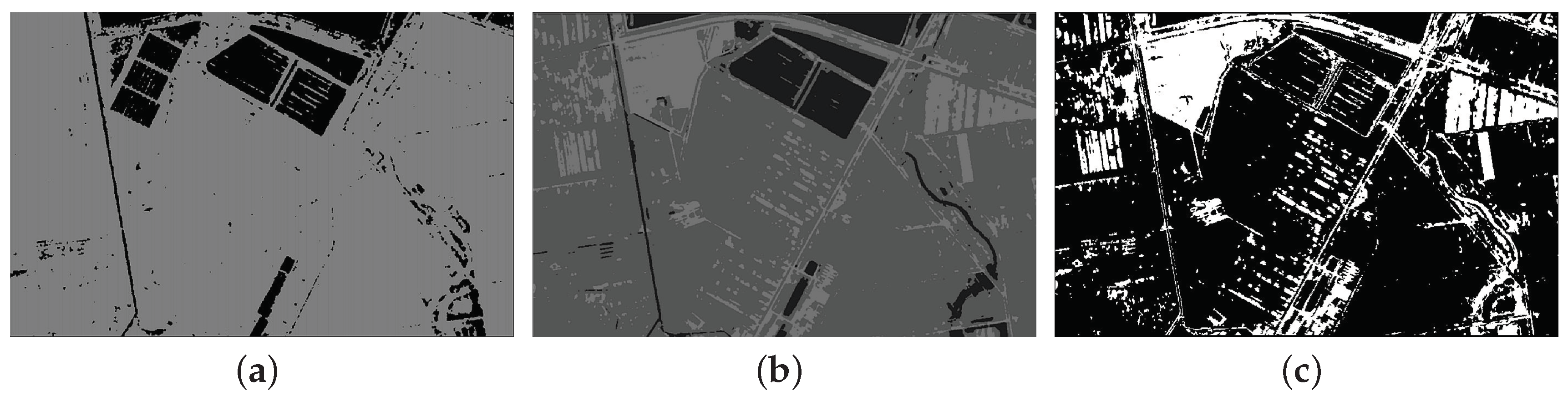
Classification and change detection maps for the Yellow River dataset by PCC. (a) Classification image for the SAR image. (b) Classification image for the optical image. (c) Resulting image.
Figure 17.
Classification and change detection maps for the Yellow River dataset by PCC. (a) Classification image for the SAR image. (b) Classification image for the optical image. (c) Resulting image.

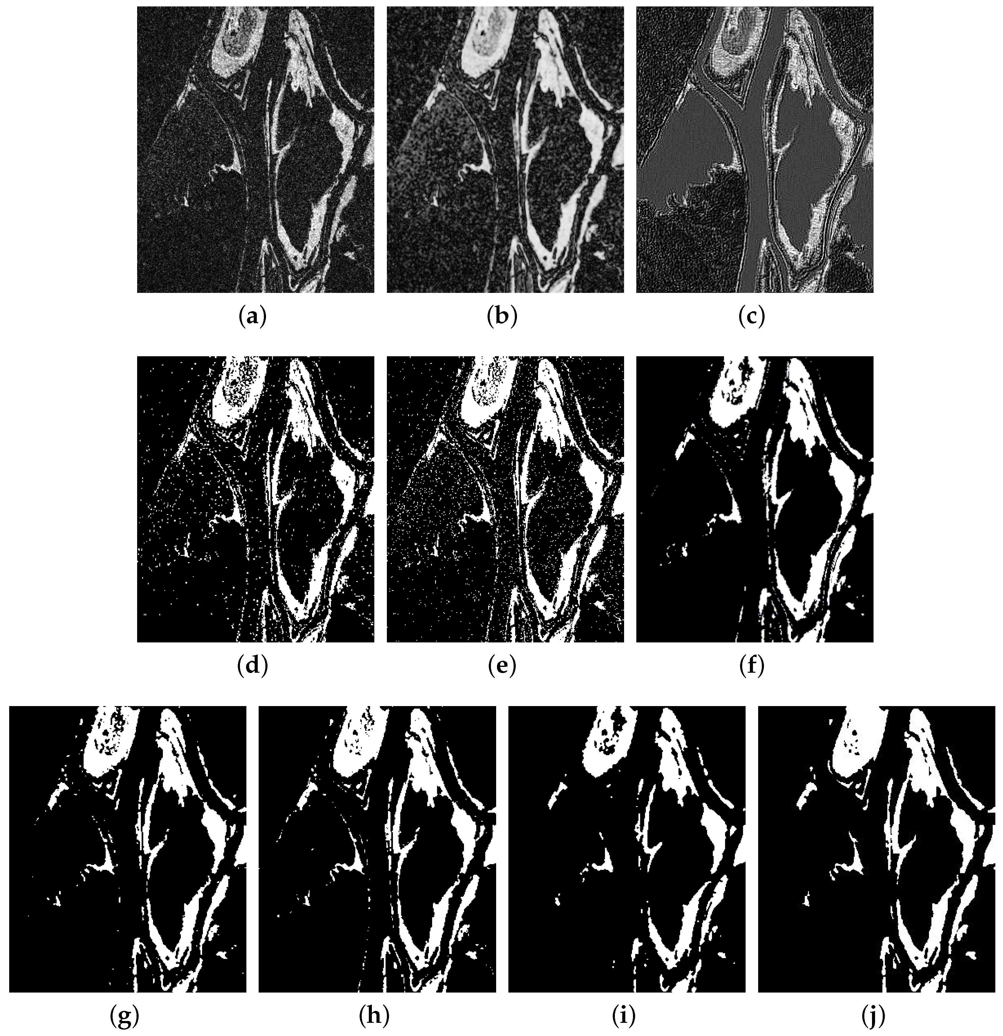
Figure 18.
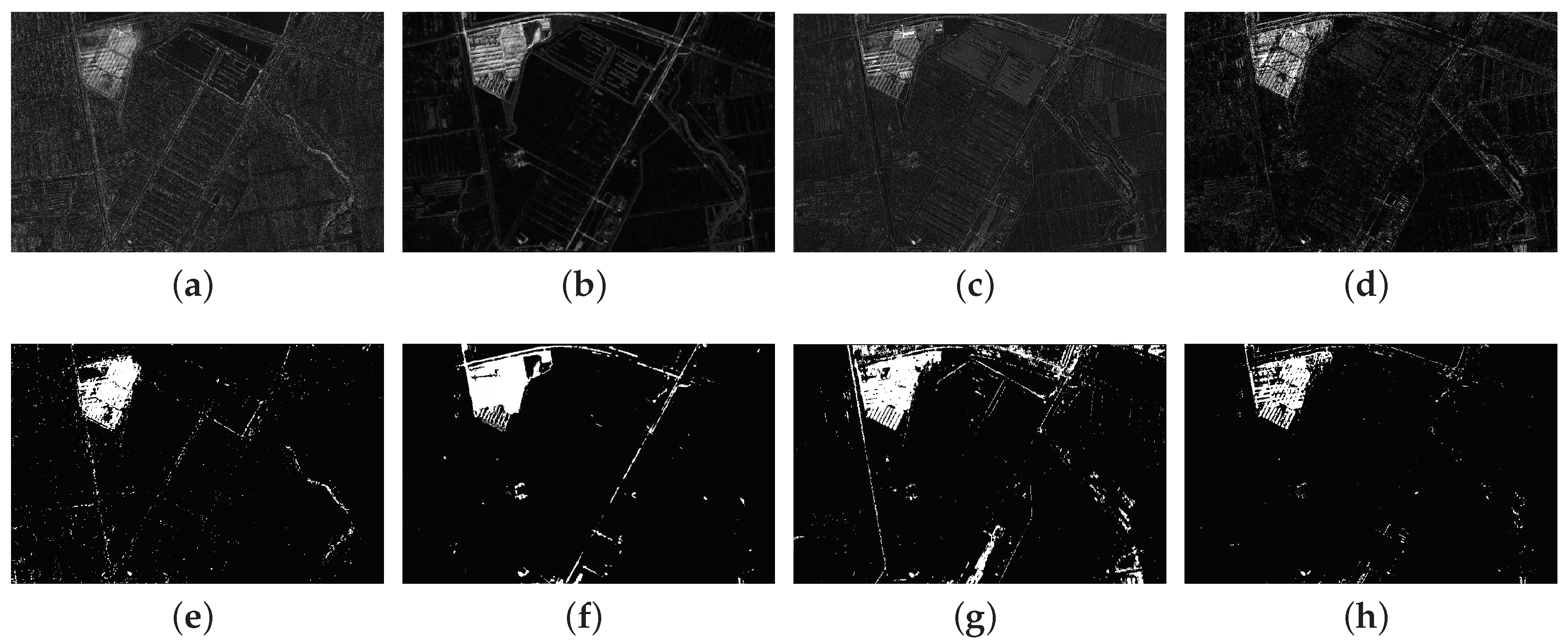
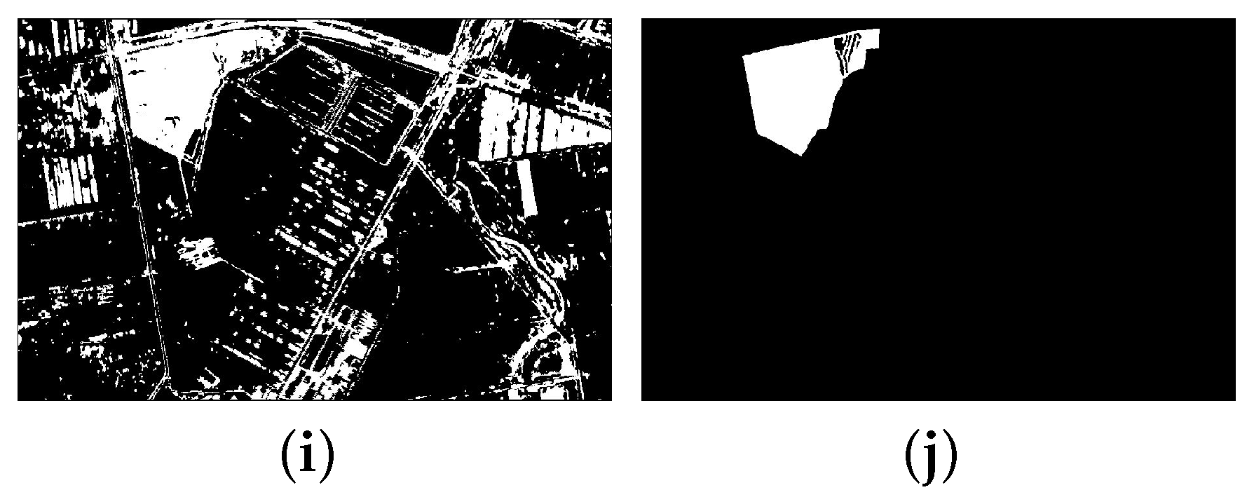
Difference images and resulting images for the Yellow River dataset obtained by different methods. (a) Difference image by change vector analysis (CVA). (b) Difference image by ASDNN. (c) Difference image by SCCN. (d) Difference image by our proposed method. (e) Resulting image by CVA. (f) Resulting image by ASDNN. (g) Resulting image by SCCN. (h) Resulting image by our proposed method. (i) Resulting image by PCC. (j) Reference image.
Figure 18.
Difference images and resulting images for the Yellow River dataset obtained by different methods. (a) Difference image by change vector analysis (CVA). (b) Difference image by ASDNN. (c) Difference image by SCCN. (d) Difference image by our proposed method. (e) Resulting image by CVA. (f) Resulting image by ASDNN. (g) Resulting image by SCCN. (h) Resulting image by our proposed method. (i) Resulting image by PCC. (j) Reference image.

Figure 19.
The difference images for the Shuguang Village dataset obtained according to different numbers of selected pixels. (a) Difference image when the number is . (b) Difference image when the number is . (c) Difference image when the number is . (d) Difference image when the number is . (e) Difference image when the number is . (f) Difference image when the number is .

Figure 20.
The overall error () on the Shuguang Village dataset according to different numbers of pixels selected.
Figure 20.
The overall error () on the Shuguang Village dataset according to different numbers of pixels selected.

Figure 21.
Classification and change detection images for the Shuguang Village dataset by PCC. (a) Classification image for the SAR image. (b) Classification image for the optical image. (c) Resulting image.
Figure 21.
Classification and change detection images for the Shuguang Village dataset by PCC. (a) Classification image for the SAR image. (b) Classification image for the optical image. (c) Resulting image.

Figure 22.
Difference images and resulting images for the Shuguang Village dataset obtained by different methods. (a) Difference image by CVA. (b) Difference image by ASDNN. (c) Difference image by SCCN. (d) Difference image by our proposed method. (e) Resulting image by CVA. (f) Resulting image by ASDNN. (g) Resulting image by SCCN. (h) Resulting image by our proposed method. (i) Resulting image by PCC. (j) Reference image.


Table 1.
Values of the evaluation criteria on the farmland dataset by different methods and these methods based on the deep capsule network.
Table 1.
Values of the evaluation criteria on the farmland dataset by different methods and these methods based on the deep capsule network.
| Method | FN | FP | OE | CA | KC |
|---|---|---|---|---|---|
| LR | 1989 | 2743 | 0.0531 | 0.9469 | 0.5528 |
| MR | 1160 | 1214 | 0.0267 | 0.9733 | 0.7559 |
| SCCN | 953 | 884 | 0.0206 | 0.9794 | 0.7936 |
| D_LR | 1207 | 1015 | 0.0250 | 0.9750 | 0.7679 |
| D_MR | 940 | 864 | 0.0202 | 0.9798 | 0.8160 |
| D_SCCN | 786 | 765 | 0.0174 | 0.9826 | 0.8436 |
Table 2.
Values of the evaluation criteria on the Ottawa dataset by different methods and these methods based on the deep capsule network.
Table 2.
Values of the evaluation criteria on the Ottawa dataset by different methods and these methods based on the deep capsule network.
| Method | FN | FP | OE | CA | KC |
|---|---|---|---|---|---|
| LR | 3309 | 1563 | 0.0480 | 0.9520 | 0.8171 |
| MR | 5055 | 9418 | 0.1426 | 0.8574 | 0.5908 |
| SCCN | 2686 | 1217 | 0.0424 | 0.9576 | 0.8369 |
| D_LR | 1790 | 688 | 0.0244 | 0.9756 | 0.8957 |
| D_MR | 654 | 2523 | 0.0313 | 0.9687 | 0.8061 |
| D_SCCN | 710 | 1634 | 0.0231 | 0.9769 | 0.9148 |
Table 3.
Values of the evaluation criteria on the Yellow River dataset by different methods.
| Method | FN | FP | OE | CA | KC |
|---|---|---|---|---|---|
| CVA | 2795 | 20545 | 0.2338 | 0.7662 | 0.0057 |
| ASDNN | 1068 | 1782 | 0.0284 | 0.9716 | 0.6086 |
| PCC | 1017 | 2863 | 0.0389 | 0.9611 | 0.5064 |
| SCCN | 620 | 2903 | 0.0353 | 0.9647 | 0.5513 |
| PROPOSED | 1029 | 1446 | 0.0248 | 0.9752 | 0.6220 |
Table 4.
Values of the evaluation criteria on the Shuguang Village dataset by different methods.
| Method | FN | FP | OE | CA | KC |
|---|---|---|---|---|---|
| CVA | 8522 | 6106 | 0.0268 | 0.9732 | 0.6405 |
| ASDNN | 1211 | 12,115 | 0.0244 | 0.9756 | 0.7469 |
| PCC | 489 | 97,258 | 0.1790 | 0.8210 | 0.2569 |
| SCCN | 15,751 | 20,300 | 0.0477 | 0.9523 | 0.5563 |
| PROPOSED | 2027 | 10,135 | 0.0218 | 0.9782 | 0.7214 |
© 2019 by the authors. Licensee MDPI, Basel, Switzerland. This article is an open access article distributed under the terms and conditions of the Creative Commons Attribution (CC BY) license (http://creativecommons.org/licenses/by/4.0/).
Share and Cite
MDPI and ACS Style
Ma, W.; Xiong, Y.; Wu, Y.; Yang, H.; Zhang, X.; Jiao, L. Change Detection in Remote Sensing Images Based on Image Mapping and a Deep Capsule Network. Remote Sens. 2019, 11, 626. https://doi.org/10.3390/rs11060626
AMA Style
Ma W, Xiong Y, Wu Y, Yang H, Zhang X, Jiao L. Change Detection in Remote Sensing Images Based on Image Mapping and a Deep Capsule Network. Remote Sensing. 2019; 11(6):626. https://doi.org/10.3390/rs11060626
Chicago/Turabian StyleMa, Wenping, Yunta Xiong, Yue Wu, Hui Yang, Xiangrong Zhang, and Licheng Jiao. 2019. "Change Detection in Remote Sensing Images Based on Image Mapping and a Deep Capsule Network" Remote Sensing 11, no. 6: 626. https://doi.org/10.3390/rs11060626
Note that from the first issue of 2016, this journal uses article numbers instead of page numbers. See further details here.