Article

Earth and Rock-Filled Dam Monitoring by High-Resolution X-Band Interferometry: Gongming Dam Case Study

1
Global Navigation Satellite System (GNSS) Research Centre, Wuhan University, Wuhan 430079, China
2
GFZ German Research Centre for Geosciences, Department of Geodesy, Section of Remote Sensing, 14473 Potsdam, Germany
3
Institute of Photogrammetry and GeoInformation, Leibniz University Hannover, 30167 Hannover, Germany
4
Shenzhen Water Science and Technology development company, Baoan Nan road, Shenzhen 518000, China
5
School of Water Resources and Hydropower, Wuhan University, Wuhan 430072, China
*
Authors to whom correspondence should be addressed.
Remote Sens. 2019, 11(3), 246; https://doi.org/10.3390/rs11030246
Submission received: 27 December 2018 / Revised: 21 January 2019 / Accepted: 22 January 2019 / Published: 26 January 2019
(This article belongs to the Section Remote Sensing Image Processing)

Abstract

:
Middle-sized earth- and rock-filled dams with clay cores continue to settle by approximately 0.5–1.5% of their height for approximately 1–3 years after their construction phase. This paper investigates the use of high-resolution spaceborne Synthetic aperture Radar (SAR) interferometry to monitor this settlement process, with the case of the Gongming dam in China. The varieties of slope foreshortening and stretching in the radar coordinates are attributed to the radar’s local incidence angle and the dam’s slope heading, which are analysed in detail. Focusing on the embankment slope settlement analysis, the equations for calculating foreshortening and the line-of-sight deformation decomposition are derived in detail for the adjustment and data fusing. The scattering characteristics of different materials on the dam surface are analysed, including the grass slope, concrete slope, top road (crest), top wall, step, and ditch. According to the analysis of the precipitation data from a local meteorological station, the coherence losses on the slopes are mainly caused by surface moisture. Both the TerraSAR-X Spotlight (TSX-SL) data and the COSMO-SkyMed Strip Mode (CSK-SM) data are analysed by the stacking method to assess the slopes’ deformations. The TSX-SL data results show the highest rate of settlement as 2 cm/yr on the top of the dam slope, consistent with the clay core shrinking process. The CSK-SM data show a similar trend in the lower part of the dam slope but underestimate the deformation in the upper part of the slope.

Graphical Abstract

1. Introduction

Currently, spaceborne interferometrical Synthetic aperture Radar (InSAR) is an established technique to assess ground surface deformation for a wide range of applications related to natural and man-made hazards [1,2,3]. With the developments in data processing techniques and the launch of high-resolution Synthetic aperture Radar (SAR) sensors, such as TerraSAR-X and COSMO-SkyMed, an alternative method for monitoring dam deformation based on SAR imagery became available for the engineering and surveying community. However, there have been relatively few studies examining the full potential of spaceborne InSAR for dam stability analysis. Examples include the big concrete gravity dams in three gorge dams in China [4]; the big concrete face rock-fill dam (CFRD) in Shuibuya, China [5,6]; the big arch dam in Pertusillon, Italy [7]; some big earth- and rock-filled dams with clay cores, such as those in Mosul [8] and Darbandikhan [9] in Iraq, Mornos in Greece [10], and Disueri [11] and Conza della Campania in Italy [12]; and the Masjed–Soleyman dam in Iran [13]. Additionally, several red mud dams in Hungary (small tailing dam) were monitored by the Multi-Temporal Interferometric (MTI) method [14,15]. The SAR data sets used in those cases include Envisat, ALOS, COSMO, TerraSAR, and Sentinel-1. The InSAR time-series methods of Persistent Scatterer (PS) [16] and Small Baseline Subset (SBAS) [17] are the main tools for all these case studies, as the PS and Distributed Scatterer (DS) [18] points on the dams are key for precise deformation analysis and comparison with traditional surveying techniques, such as GPS and levelling.
Due to the lower spatial resolution of the Envisat and Sentinel-1 satellites, it is difficult to assess the precise location of PS points on the dams [4,5,6,7]. In most of the case studies, the line-of-sight deformation obtained by InSAR measurements shows reasonable consistency with the traditional surveys [7,8,11] or the settlement model of the dam design [5,6,13]. It is important to use spaceborne SAR for monitoring the dam deformation when destabilization is possible due to man-made [8] or natural causes [4]. Moderate resolution Sentine-1 interferograms showed deformation of the Darbandikhan dam following the earthquake on 12 November 2017 [9] but failed to map the deformation that occurred during the earthquake due to the large-gradient of the displacement in the crest. Due to the volume dissolution of the core clay, such as in the Mosul dam [8] and Masjed–Soleyman dam [13], the line-of-sight deformation in this case was composed of both horizontal deformation and settlement of the slopes. The 233 m high Shuibuya dam experienced a post-construction settlement of more than 20 cm on the top in the first year after the completion of the dam [5,6]. The ALOS-1 data, which has a 23.6 cm wavelength, is able to retrieve information on such large deformations with root mean square (RMS) error within 1.5 cm/year. The latest dam collapse in Laos [19] shows that the middle-size dams need to be monitored immediately following their construction. The first historically documented settlement-induced dam break happened in 1916 which influenced the modern earth–rock-filled dam design and construction [20]. The dam deformation surveillance from the space will provide important insight for authorities involved in dam operation and security.
The InSAR analysis of the Masjed–Soleyman dam [13] showed that high resolution TerraSAR-X Spotlight (TSX-SL) X-band interferograms provide a complete, detailed picture of the occurrences on the crest and embankment, which cannot be observed by the interpolated results derived from GPS or levelling benchmarks. It also showed the limitation of the SAR foreshortening and the rapid deformation on the dam top that may cause squeezing of the fringes on the dam surface in near-range geometry. Earth- and rock-fill on the slope with no vegetation on the surface resulted in good quality interferograms and good results in the Masjed–Soleyman dam.
The scattering characteristics of objects are key parameters that affect both the radar reflection and the phase quality in interferograms. Bambler and Eineder [21] examined the complex scattering performance of the Gizeh pyramid in TSX-SL SAR images. In descending orbit, the east pyramid face is in the near-range geometry and forms a special dihedral reflection caused by the stone steps, which caused the interferometric phase to be invisible, and the west pyramid face is in the radar’s far-range geometry and forms a shadowed area. The interferometric phase is only visible on the north and south faces, which is consistent with the pyramid’s height.
Similar to the pyramid case, the geometry of earth- and rock-filled dams is known. The dam exhibits a hill or bank shape with two faces towards the radar beam. In this paper, we investigate in detail the reflection of the dam faces and the facilities on the dams, such as roads, steps, drainage ditches, and the top wall. Currently, there are more than 98,000 dams in China [22], 90% of which are middle-sized earth- and rock-filled dams [23]. More dams are in the planning phase of construction by Chinese companies in eastern and southern China, especially in those areas located on the ancient Silk Road, for water power supply and irrigation. This paper analyses the use of high-resolution InSAR technology for assessing dam deformation immediately following dam construction. Such monitoring is important, as it can provide insight into dam stability, with the dynamic assessment of foundation materials and their mechanical parameters. The analysis is performed using high-resolution TSX-SL data and CSK-SM data over Gongming dam, a bank-shaped embankment dam in Shenzhen, China. The comparing of the TSX-SL and CSK-SM data is also important for future engineering projects, which need the most reliable results possible.

2. Geometric Projection of SAR and Decomposition of the Dam Settlement

By knowing the geometry of the dam faces and the SAR payload parameters, the following equations in this section can be used to calculate the distortions caused by foreshortening and shadowing. The settlement-induced deformation on the dam slopes can be decomposed into the radar line-of-sight deformation by the local incidence angle, the dam azimuth angle, and the slope angle following Equation (7). The deformation results derived from the InSAR time series are in the radar line-of-sight direction, which should be adjusted by the slopes’ angle, local incidence angle, and azimuth direction.

2.1. Slope Geometry Distortion

The local topography and the geology of the ground basement are influential factors [23] for the construction of embankment dams. Therefore, most dams, although having a common geometrical configuration, vary in their detailed geometrical structures from one place to another. Embankment dams generally exhibit the shape of a bank or hill, with the upstream slope facing the water and the downstream slope with steps and a paved top road for routine checking. Typically, the slope angle is not designed to be constant, due to the earth and rock material characters and basement geology. Without the loss of generality, this paper takes a triangular prism with a 20 degree slope angle as an example of a middle-size earth- and rock-filled dam to derive the foreshortening [24], radar projection, and ground projection.
Figure 1 shows a transverse section of a middle sized dam. The left slope angle is α ; the right slope angle is β ; θ is the radar look angle; H is the dam height; γ I is the slope rate; and η α , η b , and η c are the local incidence angle of surfaces L a , L b , and L c , respectively. Neglecting the effect of the Earth’s radius and satellite height, the local incidence angle on the top surface η c is approximately equal to the look angle θ . Generally, the SAR satellite data provider will calculate the η c for the user for each frame of data.
In the hydraulic structural design field, γ is used to represent the dam slope ratio [23]. Taking the slope L a in Figure 1 as an example, the slope ratio γ 1 can be calculated by the following equation:
γ 1 = tan α = 1 2.5 = H S a
where H is the dam height, α is the slope angle, and S a is the length from point A g 1 to A g .
The local incidence angle, which is η a on the near-range slope and η b on the far-range slope, varies by the slope angle (Figure 1) and can be calculated by the following equations:
η a = η c α η b = η c + β
where η c is the local incidence angle derived from the radar height, local geodetic height, and radar look angle θ .
The length of three faces ( L a , L b , and L c ) on the dam are distorted when they are projected by the radar coordinates. The amount of distortion depends on the local incidence angle. The near-range slope face shows foreshortening, while the far-range slope face stretches compared to the ground range. Based on the geometry shown in Figure 1, the following equations can be derived:
R a = L a × sin ( η a ) R b = L b × sin ( η b ) R c = L c × sin ( η c )
In the above equations, R i ,   ( i = a ,   b ,   c ) is the radar range length of the dam slope surface. R a corresponds to the projection of the near-range slope L a , R b to the projection of the far-range slope L b , and R c to the top surface projection.
In reality, the orientation of the dam may not align completely with the radar range direction, and therefore, the effect of the satellite heading angle should be taken into consideration for calculating the distortion. As the dam only has two faces to the satellite, the distortion in the radar coordinate calculation is not more complex than that of the pyramid or other structures.
Figure 2 illustrates the real geometry for the radar imaging of a dam; ϕ is the angle between the dam transverse section and the radar range direction, α and β are the original slope angles, ω is the near-range slope angle projected to the radar range direction, and ψ is the far-range slope angle projected to the radar range. According to this geometry, we derive the following equations:
ω = tan 1 ( H S a 1 ) = tan 1 ( H S a × cos ϕ ) ψ = tan 1 ( H S b 1 ) = tan 1 ( H S b × cos ϕ )
where S a 1 is the ground range of L a 1 along the radar range direction and S b 1 follows the same rule. Due to the distortion along the radar range direction, the slope lengths of La, Lb, and Lc change to L a 1 , L b 1 , and L c 1 , respectively, by the following equations:
L a 1 = L a / cos ϕ L b 1 = L b / cos ϕ L c 1 = L c / cos ϕ
Accordingly, the local incidence angle will also change while the slope direction varies according to the radar range direction. As shown in Figure 2, when the angle between the dam transverse and radar range is ϕ , the near-range surface local incidence angle changes to η a 1 , and the far-range is η b 1 .
η a 1 = η c ω η b 1 = η c + ψ
Specifically, when ϕ = 90 ° , ω and ψ will be equal to 0. As a result, the local incidence angles will be equal to each other ( η a 1 = η b 1 = η c ).

2.2. The Surface Vertical Subsidence Projection on the Radar Coordinate

The dams’ post-construction movements are attributed to the consolidation settlement processing caused by the dams’ own weight, if there is no water impounding [23]. Figure 3 shows the vertical deformation of the dam’s slope surface and its projection on the radar coordinate. Here, the local incidence angle on the surface still plays an important role when satellite radar is used for deriving the displacement. Taking the vertical displacement of three dam surfaces as h , then the radar range displacement vector R a , R b , and R c can be calculated by the following equations:
R a = d a × cos η a = h × cos α × cos η a R b = d b × cos η b = h × cos β × cos η b R c = h × cos η c
where, d a and d b are the near-range and far-range surface displacement projected on the normal direction, respectively.
When the dam’s transverse section is not aligned with the radar beam and the intersection angle is ϕ (in Figure 2), the local incidence angles η a 1 and η b 1 should be adjusted by Equation (6). For the case in which ϕ = 90 ° , ω and ψ will equal to 0 and, as a result, R a = R b = R c .

3. Dam Location Area and SAR Processing Method

3.1. The Gongming Dam

The Gongming reservoir is composed of six dams with a total length of 4.34 km. The normal water level is planned to be approximately 60 m above sea level with a 1.42 × 10⁸ m3 water storage capacity. The normal water area is approximately 6 km2, and the catchment is approximately 11.7 km2. The number 4 dam is the highest of the dams, with a height of 50.7 m and length of 1121 m, and was completed at the beginning of 2016 (Figure 4b). It has a 50-metre-high clay core and concrete slabs on the upstream side.
Considering the height and the settlement of the dam, the total construction period of the No. 4 dam was approximately 4 years, i.e., from 2013 to 2017. After over 3 years of slow subsidence, the physical properties and structure of the fill materials on the bottom are expected to become stable. The dam’s lower part compaction due to self-weight is negligible: it is not the main component of the dam subsidence. Considering the No. 4 dam design (Figure 5) and construction process, we can conclude that after construction (since January 2017), the settlement of the dam surface is mainly induced by the upper layer dam’s newly filled materials and slow consolidation of clay cores.
Figure 5a–c shows the contour map, the longitudinal axis profile of the dam, and the transection at 235 m, respectively. Both the clay core and the concrete shell on the upper stream have been designed to achieve the safest structure possible. To ensure no serious seepage occurs in the dam basement area, a cement anti-seepage wall as high as 8 m and curtain grouting as deep as 30 m were constructed under the dam axis (shown in Figure 5b,c). The concrete face, which is 30 cm thick, was used for the upstream to resist erosion with a slope ratio of 1:3. Beneath the slope are strongly weathered stones (shown in Figure 5c).
The downstream slope of the dam is covered by greensward, consisting of an upper area with a slope of 1:2.5 and a bottom area with a slope of 1:2.75. The interior of the dam beneath the downstream area, which is filled with strongly weathered stones, is dry all year because of the high-level anti-seepage measures. Following the completion of the self-weight induced settlement (usually 2–3 years), the slope will be steady [23]. After that, there will be no obvious subsidence. For the stability of the downstream slope, a 6-m-high enrockment triangular prism filled with big stones has been designed. Figure 5c shows the transection at 235 m. As observed in this figure, the clay core wall with a slope of 1:0.5 is very thick and is surrounded by coarse sand filter layers as thick as 0.3 m. Considering the physical properties of the material, the subsidence of the clay wall is higher than the rock-fill body and may last for several years. Thus, the clay core contributes to the greatest subsidence after the dam construction.
Similar to the technology of traditional concrete-facing rock-fill dams, the upstream is composed by joined concrete boards to resist the water wave erosion, which are 3 × 3 m2 in size and are 30 cm thick. Each concrete board has at least 8 small holes for the water inflow. The thick clay core is the key for the water leakage. Once the impoundment process starts, the water load pressure on the dam body will cause horizontal and vertical deformation.
As traditional surveying techniques, such as levelling and total station, are costly and have low efficiency; most of the middle-sized earth–rock-filled dams do not implement surface deformation monitoring during construction [23]. Gongming dam has not experienced the surface deformation since the main part of construction has been accomplished. In 2018, the local management began to monitor the dam surface deformation by Global Navigation Satellite System (GNSS), levelling, and total station, while several benchmarks had been performed on the dam slope at that time.

3.2. SAR Data Parameters

In this paper, we analysed TSX-SL and CSK-SM SAR images covering the Gongming dam area both in ascending and descending orbit (Figure 4 shows the coverage of those data). Table 1 shows the main parameters of those SAR images.
For the TSX-SL data sets, there are 5 ascending scenes with an incidence angle of 36° and a heading angle of 350°, as well as 5 descending scenes with an incidence angle of 39° and a heading angle of 190°. The radar range resolution is 0.45 m and the azimuth resolution is 0.86 m.
For the CSK-SM data sets, there are 13 ascending images and 17 descending ones. Their incidence angle and heading angle are slightly different than the TSX-SL data. However, the radar range resolution is approximately 1.2 m and azimuth resolution is approximately 2 m, which are nearly 3 times bigger than those of the TSX-SL data.
The polarization of the CSK-SM data is HH, while that of the TSX-SL is VV. The difference in the polarization may cause the difference on the intensity of the SAR images and the coherence of the interferograms, especially for the dihedral reflection. TSX-SL and CSK-SM are two different satellite platforms with different focusing modes, so we cannot directly compare their polarization changes.

3.3. Stacking Method

This paper used the stacking method [25,26] to deal with the TSX-SL data differential interferograms time series. The processing was done using the software package RapidSAR, which was developed at the Wuhan University using MATLAB code. Before stacking the interferograms, the Goldstein filter was used to decrease the noise of each differential interferograms and the minimum cost flow (MCF) phase unwrapping method was used to derive the line-of-sight (LOS) displacement maps. Pixels with coherence values greater than 0.4 were considered as Coherence Points Candidates (CPC). Only the CPC data sets are taken into account in the interferogram matrixes. The following equation is used for the inversion of unwrapped data:
AV = obs · A = [ t 1 t 1 t 2 t N 1 ] , V = [ v 1 v 2 v N 1 ] , obs = [ 1 2 M ]
where A is the coefficient matrix containing the time interval of each interferogram t i ; t i = T i + 1 T i ; T i is the number i SAR image acquisition time i [ 1 , N 1 ] ; N is the SAR data numbers; V is the deformation rate (yearly); V i is the deformation rate between the number i and number i + 1 SAR image; obs is the interferogram phase matrix; and M is the number of interferograms.
Using the singular value decomposition (SVD) method to decompose the matrix in Equation (8), the deformation rate between every two interferograms could be solved by the matrix V . Then, the accumulated phase of the i + 1 interferogram ( ϕ i + 1 ) can be calculated by the following equation:
i + 1 = k = 1 i t k v k
The residual error ε is estimated as follows:
ϵ = obs AV

4. Monitoring Results and Discussion

4.1. Dam Geometrical Distortion

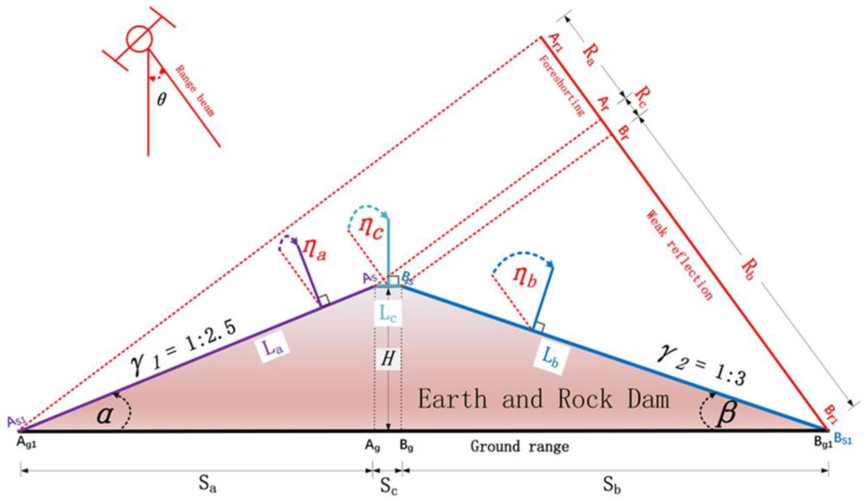
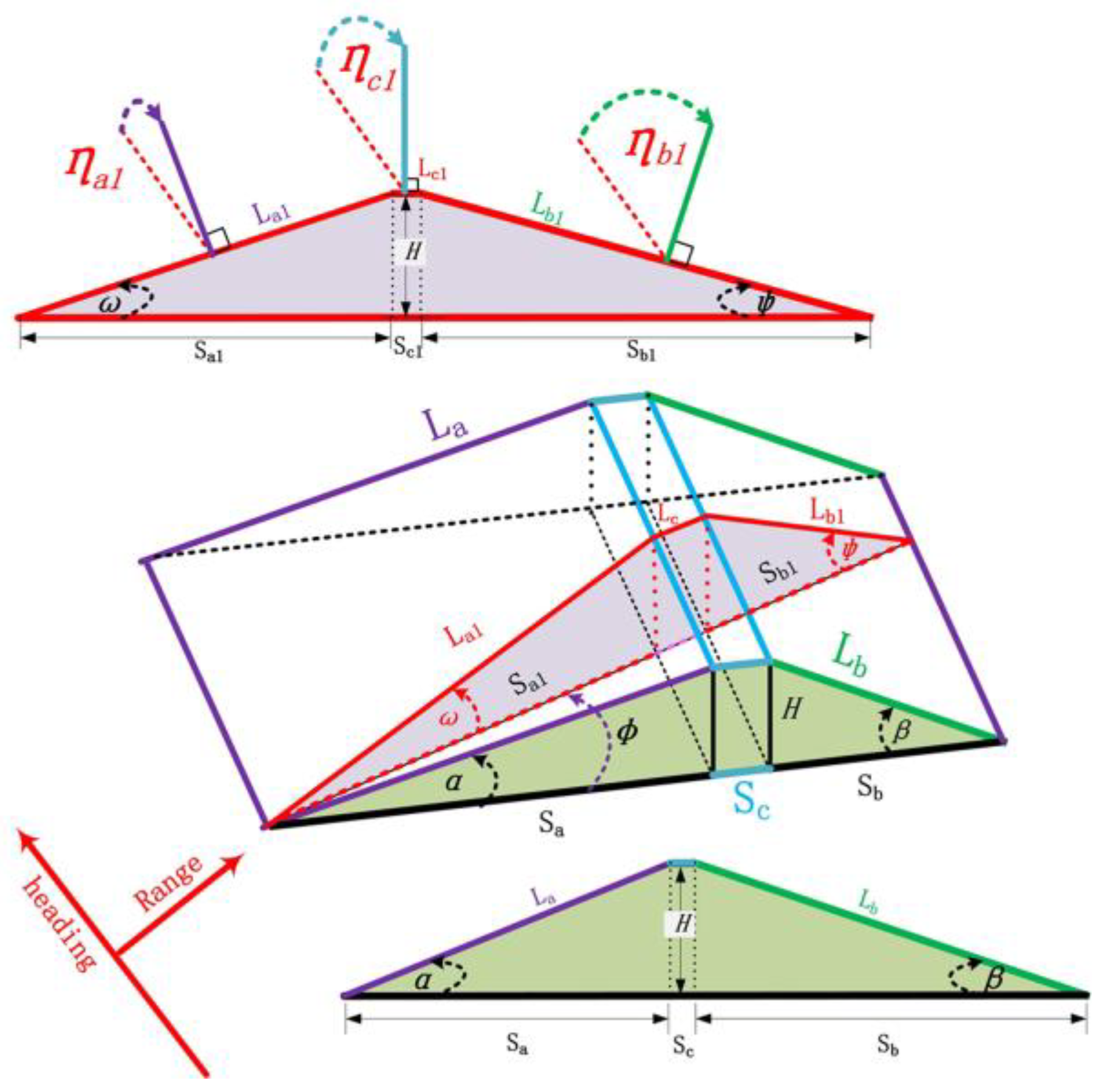
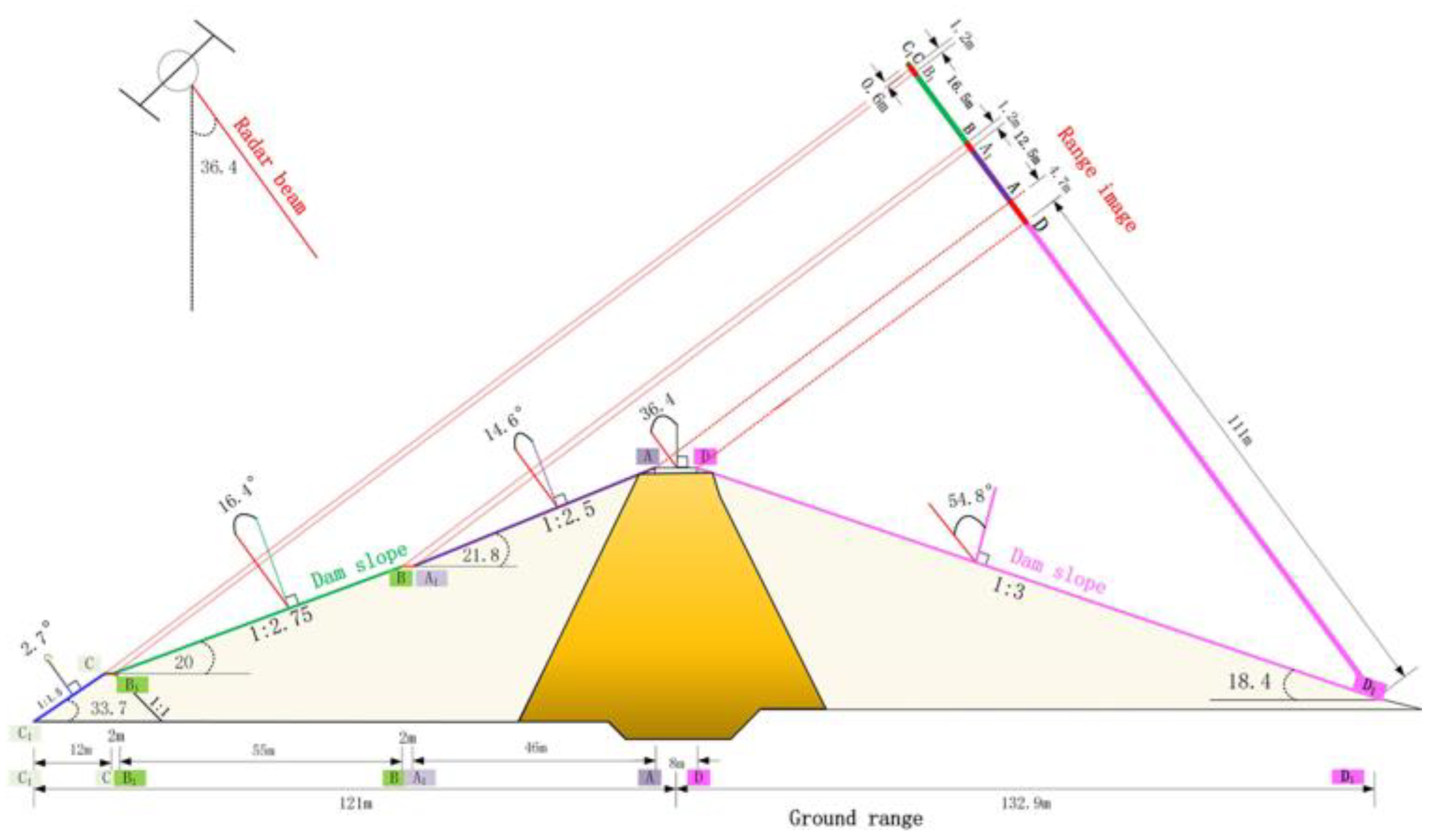
Considering the satellite parameter and the geometry of the Gongming dam 4 at the 235 m transect (Figure 6), we can calculate all the detailed parameters and variables of the slope length, slope rate, slope angle, local incidence angle, ground range, and radar range.
As shown in Table 2, the upper slope face (1:2.5) to the radar near-range with a length of 49.5 m suffers from foreshortening and decreases into 12.5 m in the radar range. Similarly, the 58.5 m lower slope face (1:2.75) is foreshortened to 16.5 m. The serious distortion occurs for the 14.4 m enrockment slope (1:1.5), which has a length of 0.6 m in the radar range, i.e., 1 pixel width. The 140.1 m long far-range slope D-D1 has been projected to 132.9 m in the ground range and to 114 m in the radar range. The 8 m width top road A-D has been projected to 4.7 m in the radar range. The 2-m-wide checking-road B-A1 between the upper slope and lower slope has been projected to 1.2 m in the radar range, nearly 2 pixels in the spotlight image.
The Gongming dam surface is composed of a variety of materials, including the upstream concrete shell slope, concrete top road, downstream grass slope, enrockment slope, plastered steps, drainage ditches, etc. In general, they all follow the Rayleigh scattering rule, such as diffuse reflection, specular reflection, and dihedral reflection. 
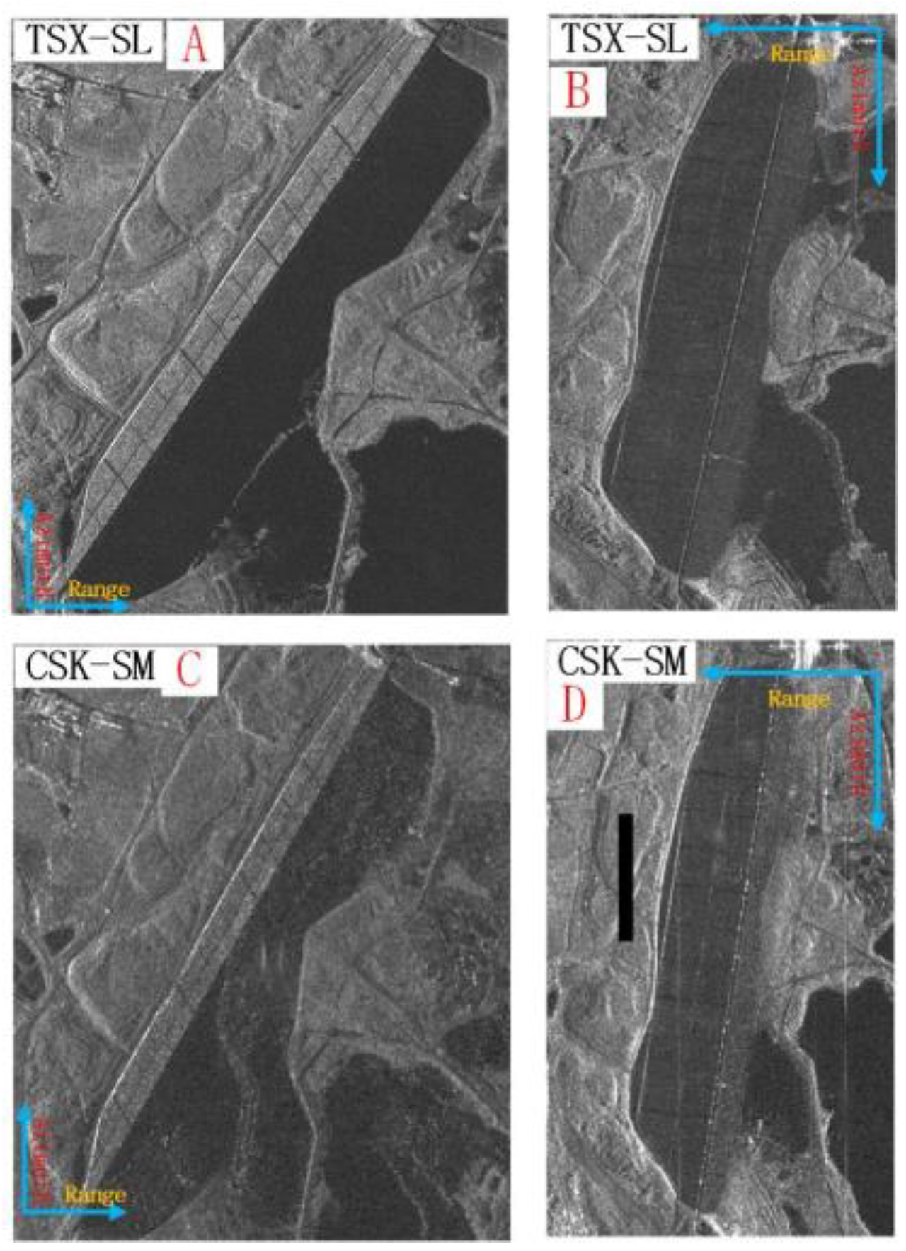
Figure 7 shows the distortion of the dam surface in real SAR images. It is clear that the downstream and upstream slopes suffer different distortions in the ascending and descending orbits, while the top road does not show much difference. For the ascending distortion, Table 2 gives the real distortion length of the slopes and roads in the 235 m transverse section, where the serious foreshortening in the radar coordinate appears on the 14.4-m-long C-C1 enrockment slope in the CSK-SM image as 0.1 pixel, while in TSX-SL image appears as 1 pixel. However, this slope still shows a very high reflection line in the ascending geometry in Figure 7. For the other slopes and the road on the dam, their radar coordinate projection pixels in the TSX-SL image is approximately 3 times shorter than the CSK-SM image.
Figure 7 shows that the TSX-SL images have better qualities and are less noisy than the CSK-SM data because of the high resolution. The averaged amplitude could also represent the phase quality of the data. The dam 4 data in TSX-SL and CSK-SM are slightly different due to the local incidence angle both in the ascending and descending orbits. In the descending orbit, the dam’s concrete slope in Figure 7B is wider than that in Figure 7D because there are 7 degrees difference in the local incidence angle (Table 1).

4.2. Dam Surface Scattering Characteristics

In the high-resolution SAR images, the dam surface materials can be discerned by their scattering features. Their geometry distortion and position could be determined through an optical image and digital elevation model (DEM). In this section, we analyse all the materials on the dams to investigate the intensity and coherence changes in the time series SAR images.
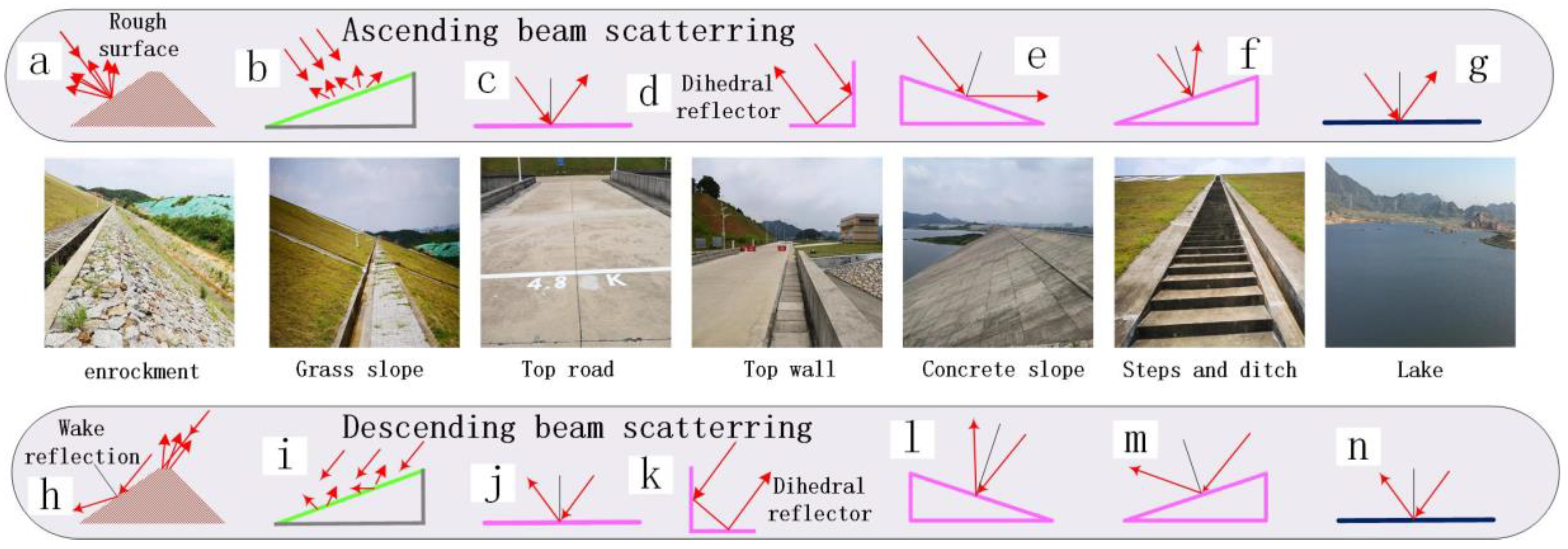
Figure 8 shows the different materials causing specific scattering for the ascending and descending data. Each small pattern shows the detailed light-in and scattering-out geometry of a type of material used on the dam. Theoretically, the concrete shell, top road, plastered steps, and drainage ditch all have smooth surfaces, which should cause specular reflection. The rough surfaces, such as the enrockment and the grass slope, will show diffuse reflection when they are facing towards the radar, that is, in near-range. The top wall of the dam could cause dihedral scattering with the right geometry along the radar side.
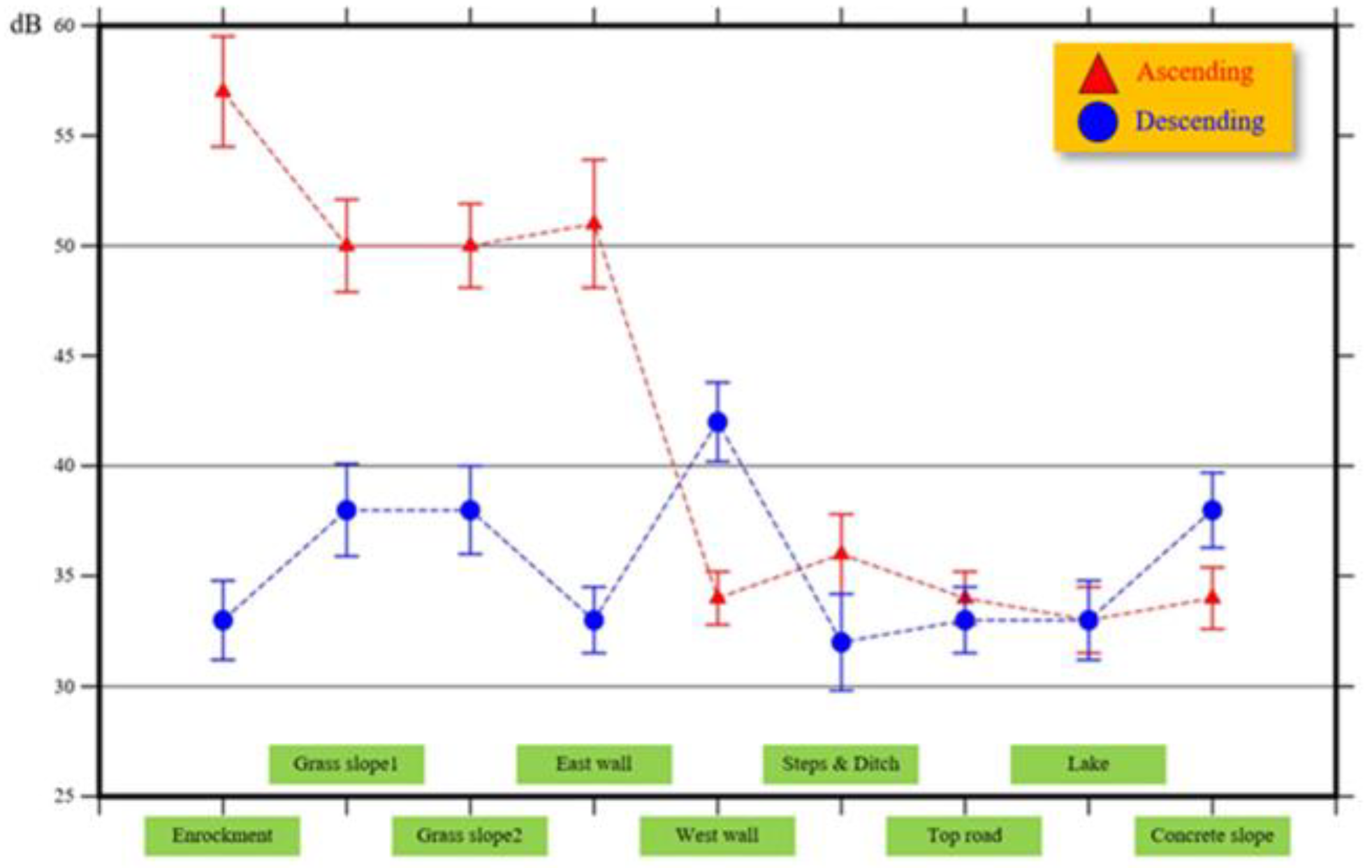
To compare the material intensity changes, Figure 9 show the TSX-SL data average intensity of all the dam surfaces in ascending and descending orbit geometry. As the CSK-SM data are too noisy, the road and steps are hard to discern: we did not count or draw them in the figure. This figure shows that the lake’s surface and the road have similar intensities at 32 dB. They can be regarded as the lowest response of the radar signal because of the specular reflection geometry. Meanwhile, the enrockment, east wall, west wall, step, and ditches may all be as dark as the lake surface in a particular geometry. The walls have dihedral reflection in the right geometry and then show higher intensity. The slope materials in our study are grass, polished rocks, and concrete slab, which the intensity of varied according to the local incidence angle and radar distortion geometry. To investigate this, we analysed the surface smoothness and the local angle of those slopes, such as the enrockment slope, grass slope, and concrete slope.
The smoothness of a surface in the radar reflection not only depends on the roughness of the material’s surface but also depends on the local incidence angle of the material surface. The approximate criteria to describe the smoothness of a surface was proposed by Rayleigh as follows [27]:
h > λ ρ × cos ( η ) ;   ρ = 8
where h is the variance of the material surface roughness (in the following, we call it maximum roughness), λ is the radar wavelength, and η is the local incidence angle of the material. For most of the materials, ρ is a constant that equals to 8; for some special materials, ρ could be 16–32.
In this paper, we assume that the grass slope and the concrete slope on the dam should follow the Equation (11) criteria. In the ascending orbit, the enrockment reflection is great, but the local incidence angle in the TSX-SL image is 2.7°, corresponding to 1 pixel in the radar range, while in CSK-SM image, the angle is 0.3° and corresponds to 0.1 pixel (Table 2). In the TSX-SL descending orbit, the local incidence angle is 73° and the enrockment slope looks very smooth. The reason is that all the rocks’ tops have been polished and are neatly embedded. The grass slope with a 15° local incidence has a strong reflection of approximately 50 dB. When the local incidence angle changes to 60° in the descending orbit, the intensity of the grass slope decreases to 38 dB. The concrete slope has the smoothest surface, and its intensity does not change between the ascending and descending orbits. The lower intensity of the concrete slope also causes the lower correlation in the time series images.

4.2.1. Slope of the Near-Range Reflection

In the ascending orbit, the enrockment slope and the grass slope are in the near-range geometry. The enrockment slope surface formed the 2.7° local incidence angle (Figure 6) and 57 dB intensity in TSX-SL, which is the brightest object on the dam surface (Figure 7A,C). However, the small local incidence angle also causes a series of foreshortening occurrences, which compresses the 14.4-m C-C1 slope into 1 pixel in the radar coordinate. The grass slope in this geometry forms a 15–16° local incidence and 50 dB intensity in TSX-SL. The slight slope angle difference (1.8°) between the upper part and lower part did not affect their intensity, however.
In the descending orbit, the upstream concrete slope is in the near-range geometry (Figure 7B,D) with a 21° local incidence angle. The concrete boards are smooth enough with a roughness of no more than 2 mm, but its intensity is 38 dB, which is 5 dB higher than the water surface. The dielectric constant should be taken into account in this case. Additionally, the 5 dB higher contrast of the intensity also maintains the phase stability of the concrete slope in the time series.

4.2.2. Slope of the Far-Range Reflection

In the ascending orbit, the upstream concrete slope is in the far-range geometry, which has a local incidence angle of approximately 55°. It appears all in black in Figure 7A,C, with the averaged intensity of 32 dB.
While in the descending orbit, the enrockment slope and the grass slope are in the far-range geometry with very low intensities. The enrockment slope’s local incidence angle is 73°, and its averaged intensity is 33 dB. The grass slope’s local incidence angle is approximately 60°, and the intensity is no more than 38 dB. It can be inferred that the slopes in the radar’s far range always have weak reflections and poor correlations because of the smooth surfaces.

4.2.3. Top Wall Dihedral Reflection

Figure 9 shows a significate intensity change of the top wall between the descending and ascending orbits, which means that the dihedral reflection only formed between the top wall and the top road in the right geometry, shown in Figure 8d,k. In the descending orbit, the west top wall has a smaller angle between the azimuth direction and then has a 52 dB average intensity. The west top wall is only 45 cm in height, which will only be projected as 1 pixel in TSX-SL image and 0.4 pixel in CSK-SM image. While in the ascending orbit, the east top walls’ average intensity is approximately 41 dB. The east top wall is 70 cm in height, which will appear as 1 pixel in TSX-SL image and 0.3 pixel in CSK-SM image in the radar coordinates. In the dihedral reflection geometry, the west top walls’ intensity is nearly 11 dB higher than that of the east top wall, but its height is 25 cm lower, which means that the orientation of the wall is the main effect for the intensity of the dihedral reflection.

4.2.4. Horizontal Smooth Surface Reflection

The roads on the dam top and in the middle have the same intensities as the water surface, which could not preserve the phase in the interferograms. The intensity of the steps and ditches on the dam have similar values as that of the roads. The road and steps show the clear borders of the grass slope. Even in the noisy CSK-SM data, the dark road and steps can be easily classified. The lower intensity also combines with the lower coherence and no phase stability on the smooth road.

4.3. TSX-SL Differential Interferograms and Decorrelation Analysis

According to the geometry and the scattering mechanism, in the ascending orbit, we can only obtain the grass slope deformation results, while in the descending orbit, only the concrete slope deformation can be retrieved.
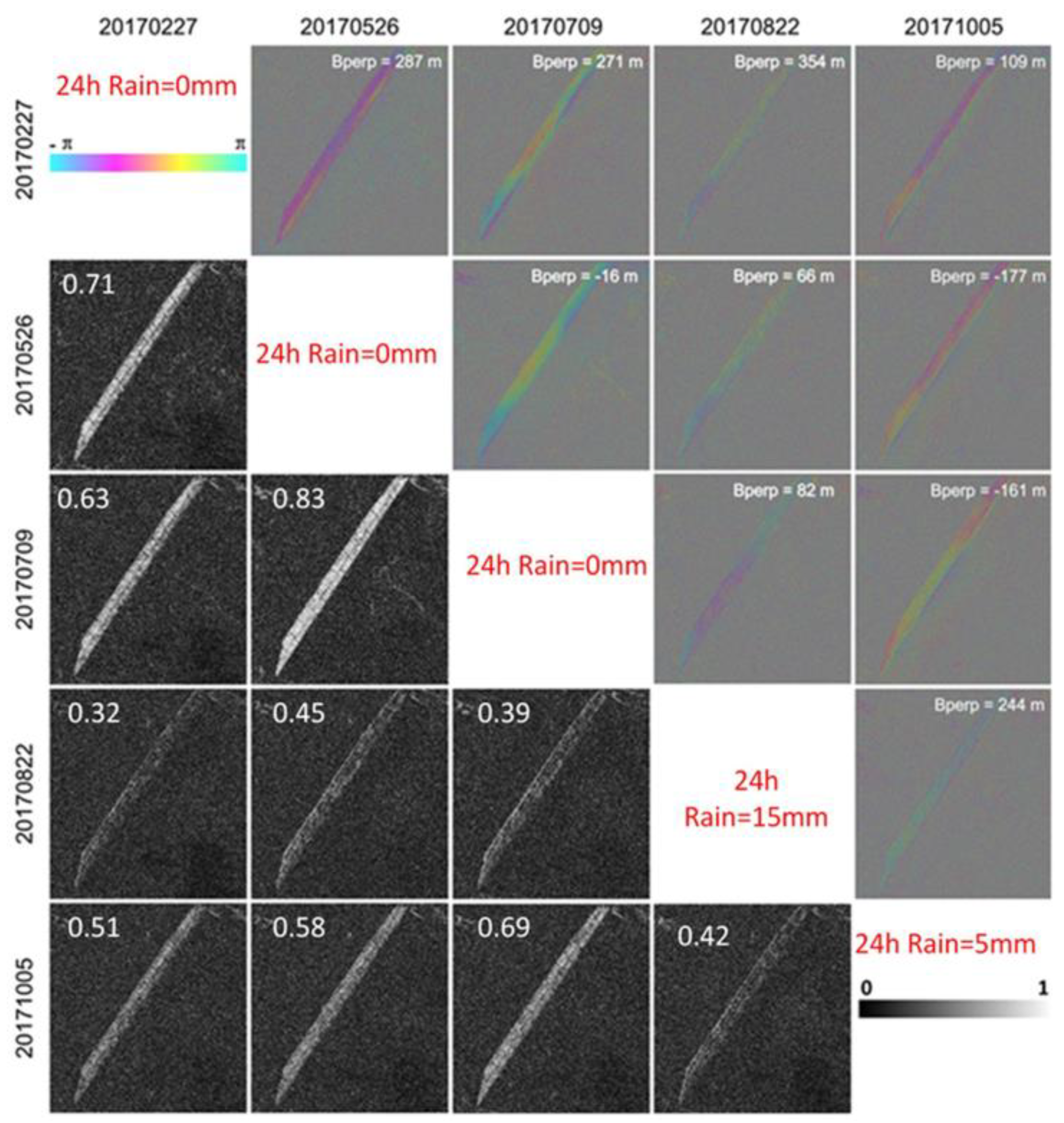
Figure 10 shows the time series of the differential interferograms in the ascending orbit in radar coordinates. The interferograms have been corrected for the effect of topography. The perpendicular baseline of those interferograms are all lower than 300 m, except for the 20170227–20170822 interferogram, which has a baseline of 354 m. That means less decorrelation may be caused by the perpendicular baseline for every interferogram. For the ascending interferograms, only the grass slope preserved the continuous phase ramp, while on the upstream concrete slope, no fringes are found. The coherence map also confirms that only the grass slope area has good correlation results higher than 0.5; all other areas are dark due to poor correlation <0.2.
The upstream concrete slope loses the coherence in all the interferograms due to the smoothness of the surface and the large local incidence angle that forms the specular reflection for the radar beam. However, as shown in Figure 10, the interferograms with 20170822 as the master image all have poor correlation to the grass slope. Inspecting the precipitation of the closest meteorology station from Shenzhen meteorology administration indicates a rainfall of 15 mm 24 h before the SAR image acquisition [28]. This suggests that the rainfall changed the grass slope surface’s moisture and the dielectric constant and accordingly decreased the correlation. The master SAR image taken in October 2017 was affected by a 5 mm rainfall. As a result, its corresponding grass slope coherence map also decreased 10% compared to other images without rain. All these observations suggest that the rain may greatly change the grass slope moisture and affect the quality of the interferometric phase.
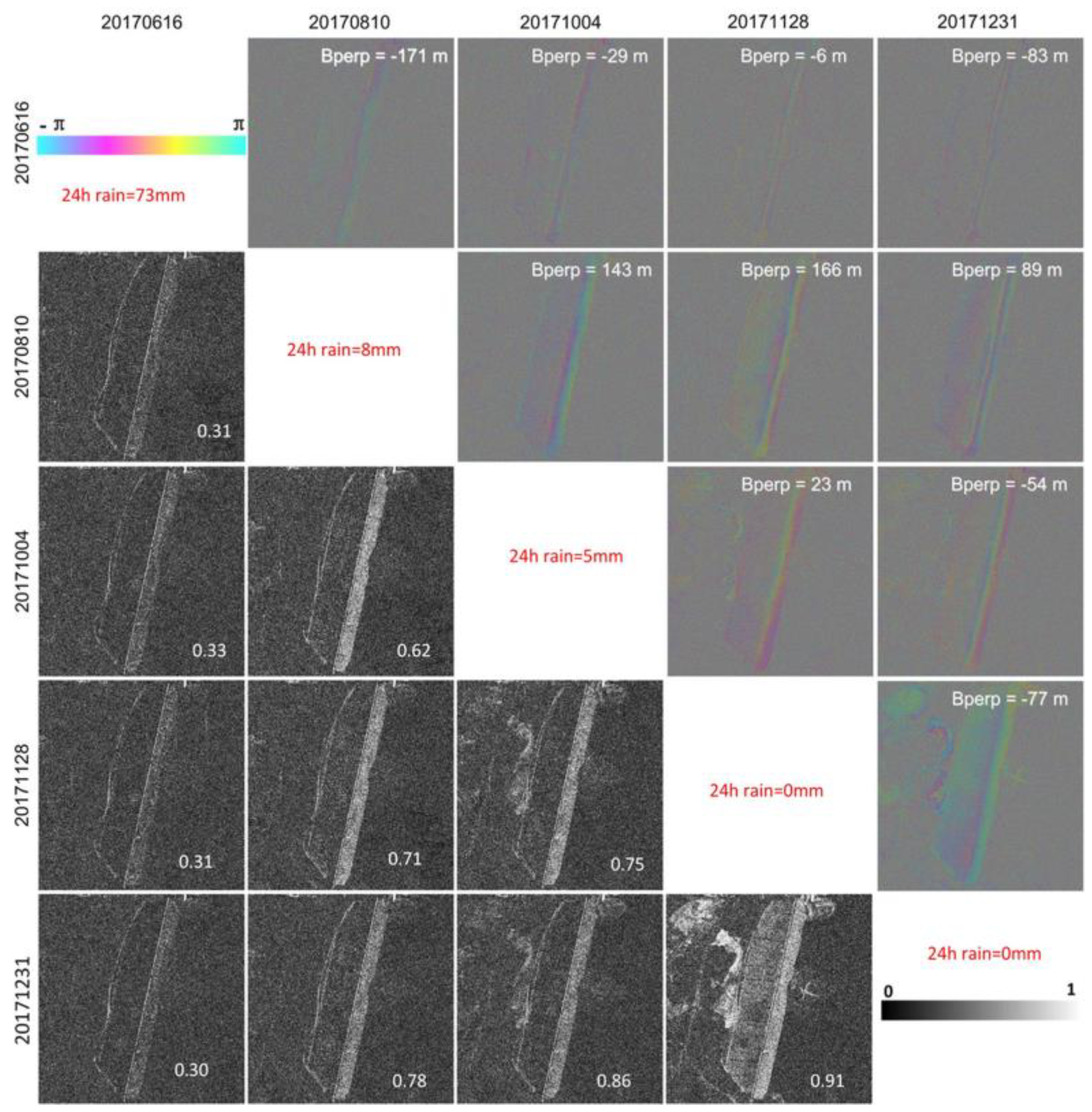
Figure 11 shows the time series of the descending differential interferograms in radar coordinates. The perpendicular baseline of those interferograms are all approximately 200 m. Theoretically, the upstream concrete slope is smooth enough for the specular reflection, while the local incidence angle is nearly 20 degrees. However, as it is in the radar near range, the 20-degree incidence angle could still reflect enough radar signal (approximately 38 dB) to maintain the stability of the phase. Meanwhile, the downstream grass slope has enough roughness with the local incidence angle of approximately 60 degrees, but the weak reflection of the radar signal (approximately 38 dB) did not create any phase in the interferograms. Three SAR images had rainfall during the acquisition, and only 2 images in the winter were not affected by rainfall. The soil moisture may have caused the loss of the correlation for all the descending interferograms series. The only exception is the coherence map 20171128–20171231, which had good coherence on the grass slope in the far-range geometry.
Although most of the descending SAR images had rainfall before the acquisition, we could still find continuous fringes on the upstream concrete slope on the interferograms. The image acquired on 16 June 2017 had the highest rainfall, with 73 mm in one day. Therefore, the pixels in the corresponding coherence map have values <0.33 (slope coherence on average).
According to the coherence maps shown in Figure 10 and Figure 11, although the heavy rainfall caused the decorrelation, it is still possible to obtain differential fringes on the SAR near-range slopes on some of the acquisitions, such as 20171005, 20170810, and 20171004. Those three SAR images have small rainfalls of no more than 8 mm, but the interferograms’ fringes and correlation maps are still good enough for the time series analysis. This means that although the dam surface’s dielectric constant may be affected by a heavy rainfall of several hours or more than one day, they may not always be low in the summer rainy season. It is still possible to have good correlation interferograms during the rainy season, which ensures the InSAR technology will be practicable for dam concrete facet monitoring in all seasons.
The differential interferogram 201701128–20171231 shows that in the winter season, which experiences less precipitation (Figure 11), the dam concrete slope shows very high coherence (0.91) and clear fringes, even in the far-range grass slope. From November to February, good quality interferograms for the far-range grass slope can be constructed. This phenomenon also shows that TSX-SL data will be more suitable in the drought period or in an arid area.
Shenzhen is located in the low latitude area, with rainy and cloudy weather conditions. The annual average rainfall is approximately 1935 mm; the maximum precipitation occurs in June, July, and August, with the monthly rainfall being higher than 300 mm. In May and September, the average rainfall is over 200 mm. The precipitation in the rest of the months does not exceed 50 mm of rainfall. The weather conditions and the dam surface material conditions are all quite different than the pyramid study in Egypt [21] and the Iran Masjed–Soleyman dam [13], where the dry wind and decayed rock maintain coherence over years. The previous study on the Shenzhen dam showed that the dam’s surface decorrelation decreased to 0.3 when the time interval was longer than 4 months in the TerraSAR strip mode interferometry [28].
The Shenzhen meteorology administration provides nearly 100 real-time meteorology stations in Shenzhen area for all the users [29]. The nearest one, Gongming meteorology station, is approximately 5 km away from the dam. In this paper, we assumed that the Gongming dam has the same rainfall as this station. Table 3 lists all the SAR image acquisition dates and the rainfall 24 h before the acquisition time.
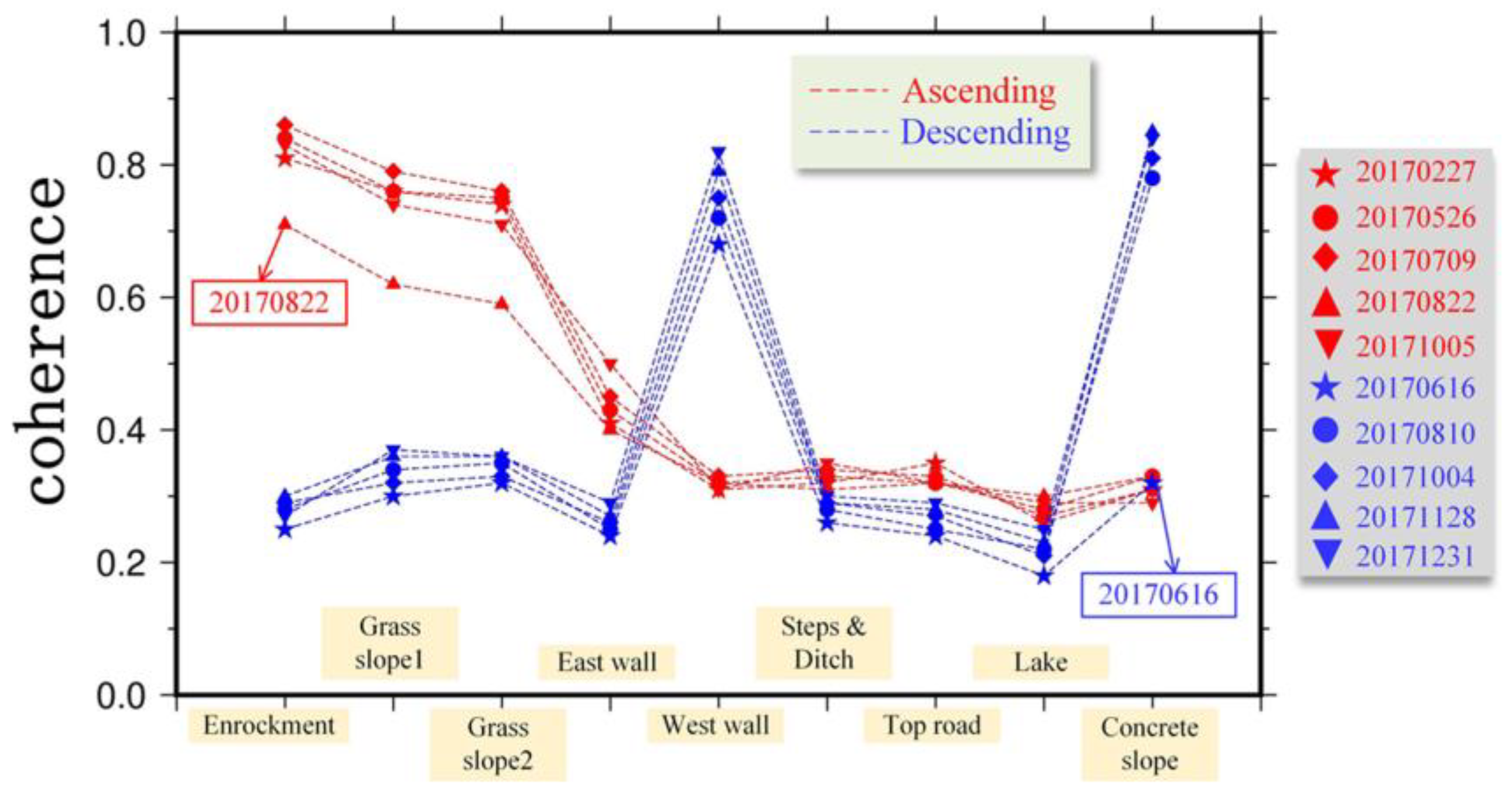
Figure 12 shows the average coherence statistics for different facets. The ascending data are shown in red, while the descending data are in blue. Then, the coherence of each facet is the average of the series coherence map. For example, taking 20170227 as the master image, we calculated the four coherence maps with 20170526, 20170709, 20170822, and 20171005. The enrockment coherence of 20170227 is then the average conference derived from these four maps.
For the ascending data, the maximum rainfall is 15 mm, which occurred on 22 August 2017. It is clear that the rainfall affects the coherence of the enrockment, grass slope 1, and slope 2. We observe around a 0.2 decrease on the correlation, which makes the interferograms noisier, as shown in Figure 12. No significant changes to the coherence are observed for the other facets on the dam, such as the top wall, steps, ditches, top road, and concrete slope, while they do not show clear fringes either.
For the descending orbit, a significant rainfall occurred on 16 June 2017 with 73 mm of rain (shown in Table 3). The rainfall greatly affects the upstream concrete slope dielectric constant, which therefore causes the decorrelation of the interferograms (Figure 12); the concrete slope’s average coherence is 0.8, which dropped to 0.3 on 20170616. However, there are no significant changes to the other material’s correlation on the dam, while they all look very low in the descending orbit.
Figure 12 shows that the top wall (east and west) does not have much decorrelation in the time series, which may be attributed to the dihedral reflection. However, more data acquisition and analysis should be done to validate the stability of the phases on the wall. The materials with lower coherence (0.3<) show that their intensity is only 1–2 dB above the water surface of the lake, which is also unable to preserve good phase stability. Neither the long baseline nor the half-year time interval decreases the correlation of the dam’s grass slope and the concrete slope. It is clear that the key contribution for coherence loss is coming from the rainfall-induced surface moisture.

4.4. TSX-SL Data Stacking Results Analysis

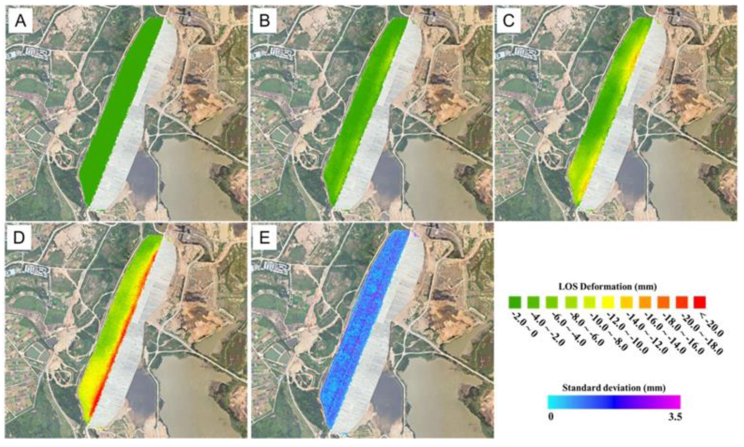
From the ascending SAR images series, over 6 months (February–October 2017), the downstream grass slope subsidence process can be derived clearly by the stacking method (Figure 13). We can see that the dam crest area shows subsidence at a rate of 3 mm/month (accumulated deformation up to −28 mm). Most of the settlement occurs in the dam crest and upper slope, suggesting that the settlement of the upper dam filling materials and clay core contributes to most of the dam deformation. The InSAR residual errors, as illustrated in Figure 13E, are approximately 1.1 mm.
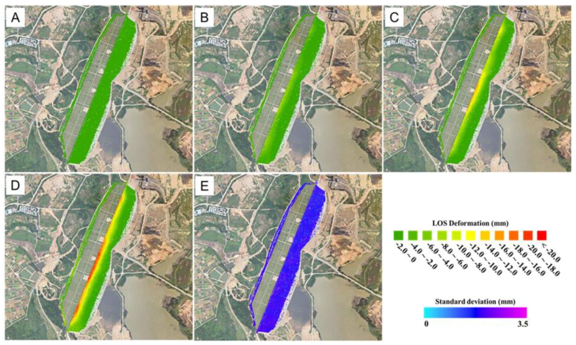
For the nearly 5 months (August–December 2017) covered by the descending TSX-SL images, the upstream concrete slope shows subsidence (Figure 14). It is clear that the main subsidence occurs in the dam crest area, deforming at a rate of 5 mm/month (accumulated deformation up to −25 mm). From the design of the dam, we know that the cement slabs are poured as 3 m × 3 m blocks, with the expansion joints filled with asphalt to avoid a thermal effect. Therefore, the interior compression of the dam could be reflected by the deformation of the cement slabs. In Figure 14E, the InSAR residuals are approximately 1.9 mm; the rainfall may affect the phase and enhance the residuals.
From the results presented, it can be concluded that the main dam settlement results from the shrinking of the clay core wall. 
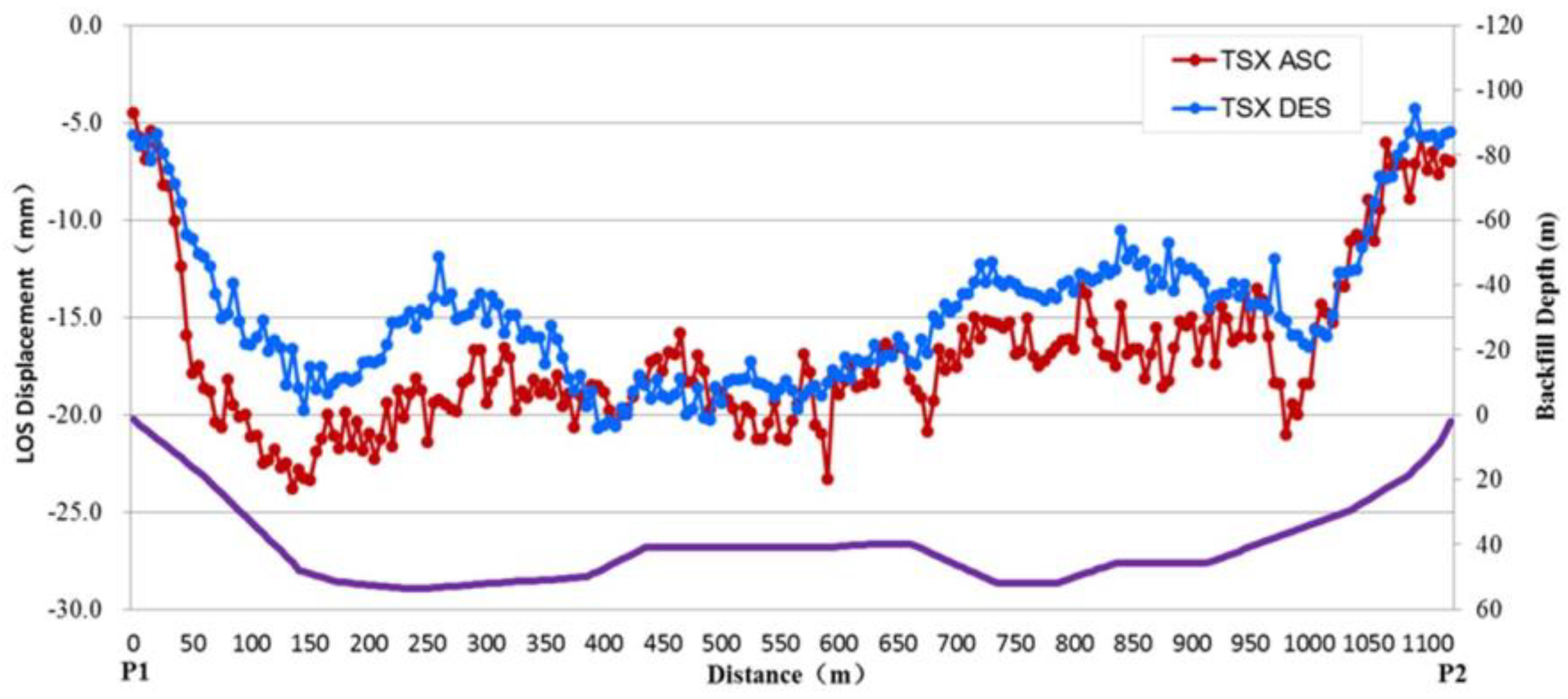
Figure 15 illustrates the changes in the total deformation trend along the axis profile of the dam (P1-P2) from the ascending and descending results with respect to the changes in the depth of the back-fill clay.
The red line in Figure 15 shows the downstream subsidence derived from the SAR data sets from 27 February to 5 October in 2017. The correlation between the centre line profile deformation and the clay core depth (magenta curve) is 0.68. This means the subsidence pattern is highly consistent with the clay depth. However, the upper part of the clay core and rock-fill area are theoretically unstable parts, which may be sinking much faster than the lower part of the dam and, therefore, contributing to the deformation in this chart. Further research needs to be performed by the numerical model of the dam material compaction.
On the other hand, the correlation between the clay core depth and the upstream subsidence is 0.62 during the 10 August and 31 December 2017 (blue line in Figure 15). The lower coefficient can be attributed to the more complicated deformation process in this facet. The tilting and the subsidence of the 3 × 3 m cement slabs may have different characteristics than the grass surface.

4.5. CSK-SM Data Stacking Results Analysis

Figure 16 shows the results of stacking obtained for ascending and descending CSK-SM images. Thirteen ascending and 17 descending images were analysed using the SBAS approach with the criteria of special baselines <300 m and temporal baseline <3 months.
The CSK-SM data sets cover a longer time interval and have more images than the TSX-SL. However, they have lower resolution, longer spatial baseline, and poor correlation. The grass slope has better coherence in CSK-SM interferograms, so the SBAS analysis provides very dense measurement points there (Figure 16a). The upstream concrete slope lost the InSAR results on the upper dam (Figure 16b) but still shows good deformation results in lower part dam.
Figure 17 shows the deformation in the grass slope on the ascending orbit, which is slightly higher than the concrete slope on the descending orbit. However, the points on the concrete slope is not at the same height of the grass slope. The grass slope on the ascending result shows a roughly linear trend. The grass slope is made by dispersing stones and soil; therefore, the deformation process follows the soil consolidation settlement process. It should be noted that according to the missing data between November 2016 and May 2017, the subsidence trend in this time interval is not very reliable.
In contrast to the grass slope, the deformation of concrete slope is not very uniform. The concrete slabs may have their own settlement processing other than the dispersing stones inside the dam. Those slabs may sustain each other and maintain the shape over some time when the inner stones have already settled.

5. Conclusions

Significant progress in monitoring infrastructures from space has been made in recent years thanks to the growing use of high-resolution radar imagery. It is important to monitor the dam deformation in its full life cycle (construction period, post-construction period, first impound period, stable period, etc.) [23], especially for the middle-sized earth- and rock-filled dams. This paper focused on the Gongming dam’s post-construction period consolidation settlement analysis by using TSX-SL and CSK-SM data.
Our results show that even with foreshortening of the embankments, it is still possible to obtain the continuous phase fringes on the dam slope both in the grass face and in concrete slab face in the dry season in the Shenzhen area. The middle-sized earth- and rock-filled dams with gentle slopes are suitable for the high-resolution D-InSAR technology while using a radar satellite with an observation angle in the range of 35–45 degrees. By analysing precipitation data, we inferred that changes in soil moisture contribute greatly to the TSX-SL data series’ coherence loss on the slopes. Fifteen mm of rainfall can seriously affect the grass slope coherence but may not have the same effect on the concrete slap. Meanwhile, 70 mm of heavy rain can completely destroy the fringe visibility and coherence on the concrete slap slope in the near-range geometry. The coherence map of each type of slope facet on the dam is helpful for detecting the poor interferograms that are affected by rainfall. This paper shows that eliminating the rainfall-affected interferograms could greatly improve the time series results. The poor quality interferograms in CSK-SM small baseline data sets are also mainly caused by the rainfall effect. Comparing the stacking results between TSX-SL and CSK-SM shows that TSX-SL data is good for monitoring the dam settlement process.
Currently, the spotlight data are only provided by missions such as TerraSAR-X and COSMO. The TSX-SL data is much better than the CSK-SM data for this small area deformation retrieval due to its high resolution and shorter baseline. In the future, the increasing availability of such high-resolution SAR data offers significant opportunities for interferometric imaging of infrastructure and understanding their movement in response to loading and triggering factors using numerical modelling [30].

Author Contributions

T.L. and M.M. conceived and designed the experiments; M.W. performed the SAR data experiments; W.Z. and L.C. analysed the data; C.G. and X.X. contributed to the dam design material analysis; J.H. contributed to the analysis of the dam deformation mechanism; J.L. contributed to the Rayleigh scattering method; T.L. wrote the original article with contribution from M.M. All authors discussed the results and commented on the manuscript.

Funding

This research was funded by the National Natural Science Foundation of China (NSFC), grant number 41674032, 41274048.

Acknowledgments

Thanks for the German Aerospace Agency (DLR) who provides the TerraSAR-X Spotlight data sets under proposal motagh_GEO1916. Thanks for Vastitude technology company who provides the COSMO-SkyMed data with the Memorandum of Understanding (MOU) between Shenzhen Water-related high technology development company. Thanks for Shenzhen Water-related high technology development company provide the dam design map and the field investigation.

Conflicts of Interest

The authors declare no conflict of interest.

References

  1. Crosetto, M.; Monserrat, O.; Cuevas, M.; Crippa, B. Spaceborne differential SAR interferometry: Data analysis tools for deformation measurement. Remot Sens. 2011, 3, 305–318. [Google Scholar] [CrossRef]
  2. Del Ventisette, C.; Ciampalini, A.; Calò, F.; Manunta, M.; Paglia, L.; Reichenbach, P.; Colombo, D.; Mora, O.; Strozzi, T.; Garcia, I.; et al. Exploitation of large archives of ERS and ENVISAT C-Band SAR data to characterize ground deformation. Remote Sens. 2013, 5, 3896–3917. [Google Scholar] [CrossRef]
  3. Antonielli, B.; Monserrat, O.; Bonini, M.; Righini, G.; Sani, F.; Luzi, G.; Feyzullayev, A.A.; Aliyev, A.S. Pre-eruptive ground deformation of Azerbaijan mud volcanoes detected through satellite radar interferometry (DInSAR). Tectonophysics 2014, 637, 163–177. [Google Scholar] [CrossRef]
  4. Wang, T.; Perissin, D.; Rocca, F.; Liao, M.S. Three Gorges Dam stability monitoring with time-series InSAR image analysis. Sci. China Earth Sci. 2011, 54, 720–732. [Google Scholar] [CrossRef]
  5. Zhou, W.; Li, S.; Zhou, Z.W.; Chang, X.L. InSAR observation and numerical modeling of the earth-dam displacement of Shuibuya Dam (China). Remote Sens. 2016, 8, 877. [Google Scholar] [CrossRef]
  6. Zhou, W.; Li, S.; Zhou, Z.W.; Chang, X.L. Remote sensing of deformation of a high concrete-faced rockfill dam using InSAR: A study of the Shuibuya Dam, China. Remote Sens. 2016, 8, 255. [Google Scholar] [CrossRef]
  7. Milillo, P.; Perissin, D.; Salzer, J.T.; Lundgren, P.; Lacava, G.; Milillo, G.; Serio, C. Monitoring dam structural health from space: Insights from novel InSAR techniques and multi-parametric modeling applied to the Pertusillo dam Basilicata, Italy. Int. J. Appl. Earth Obs. Geoinf. 2016, 52, 221–229. [Google Scholar] [CrossRef]
  8. Milillo, P.; Bürgmann, R.; Lundgren, P.; Salzer, J.; Perissin, D.; Fielding, E.; Milillo, F.B.G. Space geodetic monitoring of engineered structures: The ongoing destabilization of the Mosul dam. Iraq Sci. Rep. 2016, 6, 37408. [Google Scholar] [CrossRef]
  9. Al-Husseinawi, Y.; Li, Z.; Clarke, P.; Edwards, S. Evaluation of the Stability of the Darbandikhan Dam after the 12 November 2017 Mw 7.3 Sarpol-e Zahab (Iran–Iraq Border) Earthquake. Remote Sens. 2018, 10, 1426. [Google Scholar] [CrossRef]
  10. Spiros, N.; Panagiotis, E.; Issaak, P.; Pierre, B. Deformation estimation of an earth dam and its relation with local earthquakes, by exploiting multitemporal synthetic aperture radar interferometry: Mornos dam case (Central Greece). J. Appl. Remote Sens. 2016, 10, 10–16. [Google Scholar]
  11. Wasowski, J.; Bovenga, F.; Nutricato, R.; Nitti, D.O.; Chiaradia, M.T. High resolution satellite multi-temporal interferometry for monitoring infrastructure instability hazards. Innov. Infrastruct. Solut. 2017, 27, 1–9. [Google Scholar] [CrossRef]
  12. Di Martire, D.; Iglesias, R.; Monells, D.; Centolanza, G.; Sica, S.; Ramondini, M.; Pagano, L.; Mallorquí, J.J.; Calcaterra, D. Comparison between Differential SAR interferometry and ground measurements data in the displacement monitoring of the earth-dam of Conza della Campania (Italy). Remote Sens. Environ. 2014, 148, 58–69. [Google Scholar] [CrossRef]
  13. Emadali, L.; Motagh, M.; Haghighi, M.H. Characterizing post-construction settlement of the Masjed-Soleyman embankment dam, Southwest Iran, using TerraSAR-X SpotLight radar imagery. Eng. Struct. 2017, 143, 261–273. [Google Scholar] [CrossRef] [Green Version]
  14. Grenerczy, G.; Wegmüller, U. Persistent scatterer interferometry analysis of the embankment failure of a red mud reservoir using ENVISAT ASAR data. Nat. Hazards 2011, 59, 1047–1053. [Google Scholar] [CrossRef]
  15. Grenerczy, G.; Wegmüller, U. Deformation analysis of a burst red mud reservoir using combined descending and ascending pass ENVISAT ASAR data. Nat. Hazards 2013, 65, 2205–2214. [Google Scholar] [CrossRef]
  16. Ferretti, A.; Prati, C.; Rocca, F. Permanent scatterers in SAR interferometry. IEEE Trans. Geosci. Remote Sens. 2001, 39, 8–20. [Google Scholar] [CrossRef] [Green Version]
  17. Lanari, R.; Mora, O.; Manunta, M.; Mallorquì, J.J.; Berardino, P.; Sansosti, E. A small-baseline approach for investigating deformations on full-resolution differential SAR interferograms. IEEE Trans. Geosci. Remote Sens. 2004, 42, 1377–1386. [Google Scholar] [CrossRef]
  18. Ferretti, A.; Fumagalli, A.; Novali, F.; Prati, C.; Rocca, F.; Rucci, A. A New Algorithm for Processing Interferometric Data-Stacks: SqueeSAR. IEEE Trans. Geosci. Remote Sens. 2011, 49, 3460–3470. [Google Scholar] [CrossRef]
  19. 2018 Laos Dam Collapse. Available online: https://en.wikipedia.org/wiki/2018_Laos_dam_collapse (accessed on 10 November 2018).
  20. Raska, P.; Emmer, A. The 1916 catastrophic flood following the Bila Desna dam failure: The role of historical data sources in the reconstruction of its geomorphologic and landscape effects. Geomorphology 2014, 226, 135–147. [Google Scholar] [CrossRef]
  21. Bamler, R.; Eineder, M. The Pyramids of Gizeh Seen by TerraSAR-X—A Prime Example for Unexpected Scattering Mechanisms in SAR. IEEE Geosci. Remote Sens. Lett. 2008, 5, 468–470. [Google Scholar] [CrossRef]
  22. 2016 Statistic Bulletin on China Water Activities. Available online: http://www.mwr.gov.cn/sj/tjgb/slfztjgb/201710/t20171016_1002400.html (accessed on 25 June 2018).
  23. Hydraulic Structural Design Volume Six: Earth and Rock Filled Dam, 2nd ed.; China Water & Power Press: Beijing, China, 2014. (In Chinese)
  24. Curlander, J.C.; McDonough, R.N. Synthetic Aperture RADAR Systems and Signal Processing; Wiley: Hoboken, NJ, USA, 1991; pp. 370–410. [Google Scholar]
  25. Berardino, P.; Fornaro, G.; Lanari, R.; Sansosti, E. A new algorithm for surface deformation monitoring based on small baseline differential SAR interferograms. IEEE Trans. Geosci. Remote Sens. 2003, 40, 2375–2383. [Google Scholar] [CrossRef]
  26. Schmidt, D.A. Time-dependent land uplift and subsidence in the Santa Clara valley, California, from a large interferometric synthetic aperture radar data set. J. Geophys. Res. Solid Earth 2003, 108. [Google Scholar] [CrossRef] [Green Version]
  27. Van Zyl, J.; Kim, Y. Synthetic Aperture Radar Polarimetry; John Wiley & Sons Inc.: Hoboken, NJ, USA, 2011. [Google Scholar]
  28. Li, T.; Gong, C.; Xia, M.; Jin, Z. Analysis on coherence changes of dam surface in TerraSAR Strip mode interferograms. Proc. SPIE 2011, 8286, 8. [Google Scholar]
  29. Meteorological Bureau of Shenzhen Municipality. Available online: http://www.szmb.gov.cn/en/en_shenzhentianqi/ (accessed on 25 February 2018).
  30. Shamshiri, R.; Motagh, M.; Baes, M.; Sharifi, M.A. Deformation analysis of the Lake Urmia causeway (LUC) embankments in northwest Iran: Insights from multi-sensor interferometry synthetic aperture radar (InSAR) data and finite element modeling (FEM). J. Geod. 2014, 88, 1171–1185. [Google Scholar] [CrossRef]
Figure 1. The middle-sized earth- and rock-filled dam transverse section and radar reflection geometry.
Remotesensing 11 00246 g001
Figure 2. The dam transverse section along the radar range direction.
Remotesensing 11 00246 g002
Figure 3. The dam surface vertical deformation projecting in the radar range direction.
Remotesensing 11 00246 g003
Figure 4. Gongming dam: (A) The Google earth image as the background with TSX-SL and CSK-SM images covering the frames; the small orange box represents the number 4 dam; (B) an optical image of the number 4 dam taken by Unmanned Aerial Vehicle (UAV) in December 2016, when the main part of the dam construction was complete; P1 and P2 illustrate the dam top; (C) the topography of the number 4 dam, produced by the UAV Lidar with a 45 cm resolution in pixels and 20 cm precision in height.
Remotesensing 11 00246 g004
Figure 5. (a) A contour Map of the Gongming No. 4 dam; (b) a longitudinal axis profile map between P1 and P2; (c) a transect map at 235 m.
Remotesensing 11 00246 g005
Figure 6. The transect at (0 + 235 m) of the Gongming dam (No. 4) and its surface projection on the radar coordinate.
Remotesensing 11 00246 g006
Figure 7. The dam surface foreshortening geometry on the ascending and descending images.
Remotesensing 11 00246 g007
Figure 8. The dam surface material scattering geometry on the ascending and descending images.
Remotesensing 11 00246 g008
Figure 9. The average intensity of the dam surface in ascending and descending TSX-SL images.
Remotesensing 11 00246 g009
Figure 10. The differential interferograms and coherence map of the ascending TSX-SL images.
Remotesensing 11 00246 g010
Figure 11. The differential interferograms and coherence map of the descending TSX-SL images.
Remotesensing 11 00246 g011
Figure 12. The coherence of the dam surface changing in the TSX-SL time series.
Remotesensing 11 00246 g012
Figure 13. The deformation series results of the downstream slope in the ascending orbit TSX-SL: (A) date: 27/02/2017, (B) date: 26/05/2017, (C) date: 09/07/2017, (D) date: 05/10/2017, and (E) residual error.
Remotesensing 11 00246 g013
Figure 14. The deformation series results of the upstream slope in descending orbit TSX-SL: (A) date: 10/08/2017, (B) date: 04/10/2017, (C) date: 28/11/2017, (D) date: 31/12/2017, and (E) residual error.
Remotesensing 11 00246 g014
Figure 15. The total settlement on the dam top along the longitudinal section with clay core depth curves by TSXSL.
Remotesensing 11 00246 g015
Figure 16. The average velocity results from the CSK-SM data sets by the stacking method: (a) the downstream slope in the ascending orbit and (b) the upstream slope in the descending orbit.
Remotesensing 11 00246 g016
Figure 17. The dam top deformation series results of the CSK-SM data sets by the stacking method: (a) Points on the downstream slope in the ascending orbit and (b) Points on the upstream slope in the descending orbit.
Remotesensing 11 00246 g017
Table 1. The main parameters of the ascending and descending TSX-SL and CSK-SM data.
OrbitAscendingDescending
SensorsTSX-SLCSK-SMTSX-SLCSK-SM
Wavelength3.12 cm3.12 cm3.12 cm3.12 cm
PolarizationVVHHVVHH
Data sets517522
Period27/02/2017–
05/10/2017
2016/07/24–
2018/01/22
16/06/2017–
31/12/2017
06/06/2016–
11/05/2018
Heading349.8°349.3°190.1°190.8°
Incidence36.4°34°39.2°32.3°
Range sampling0.45 m1.18 m0.45 m1.14 m
Azimuth sampling0.86 m2.07 m0.86 m1.92 m
acquiring local time18:26 pm6:12 am + 1 day6:22 am + 1 day18:09 pm
Table 2. The parameters and variables of the slope of the Gongming dam 4 on the (0 + 235 m) transect.
Slope NameSlope RateSlope Angle (deg)Length (m)Local Incidence Angle (deg)Radar Coordinate (m)TSX-SL
Pixel
CSK
Pixel
N/F
TSX-SLCSK-SMTSX-SLCSK-SM
A-D-0836.4344.74.5104-
A-A11:2.521.849.514.612.212.510.5289N
B-B11:2.752058.516.41416.514.23712N
C-C11:1.533.714.42.70.30.60.11<0.1N
D-D11:318.4140.154.852.411411125394F
B-A1-0236.4341.21.131-
N means near-range slope; F means far-range slope; “-“ means no parameter.
Table 3. The rainfall 24 h before the TSX-SL SAR acquisition.
NumberAscendingRainfall (mm)DescendingRainfall (mm)
12017022702017061673
2201705260201708108
3201707090201710045
42017082215201711280
5201710055201712310

