Persistence of Oil Prices in Gas Import Prices and the Resilience of the Oil-Indexation Mechanism. The Case of Spanish Gas Import Prices


Escuela Técnica Superior de Ingenieros Industriales de Madrid, Universidad Politécnica de Madrid, 28006 Madrid, Spain
*
Author to whom correspondence should be addressed.
Energies 2018, 11(12), 3486; https://doi.org/10.3390/en11123486
Submission received: 21 November 2018
/
Revised: 7 December 2018
/
Accepted: 11 December 2018
/
Published: 13 December 2018
(This article belongs to the Special Issue Energy Policy and Policy Implications)
Abstract
:Regardless of the rapid development of national gas centers around the world, oil price indexation remains the prevailing pricing process in Continental Europe and the Far East. The instance of Spain is a genuine case where gas supply conditions may, to some extent, clarify the slower pace of execution of a traded gas hub in the nation. This article seeks to explain the persistence of oil-indexed pricing mechanisms, a price model that differs oddly from that of other major commodities, the price of which is normally discovered on the market. In order to do that, we examine time-varying volatility to find that since 2013 until 2016, just about 33% of gradual volatility clustering rooted within oil Brent prices is reflected in Spanish gas prices. In this sense, our research provides quantitative tools to better understand that market-based approaches such as spot and medium-term supply alternatives seem to be a key driver for success in transforming gas markets. Regular updates on the size of the effects observed should facilitate an exact appraisal of the level of progression of national gas liberalization processes and enhance gas markets transparency, these issues of extraordinary importance for both policymakers and gas market agents.
1. Introduction
With network energies traded in open markets, with many vendors and purchasers, prices are generally determined by free market activity with price itself giving signs to guarantee market balance. However, as it sometimes happens in traded markets such as electricity, limited supply of a good, coupled with high demand for that good, may result in a serious mismatch between the desired supply and demand equilibrium. Moreover, this situation would result in the exclusion of the good only to those who can afford it. In the case of gas markets and due to the nature of gas trade typically organized on the basis of regional needs, gas prices are not set everywhere under the same competitive conditions and network topology limitations may lead to very high volatility of spot prices. Furthermore, the strong push from governments for liberalization will continue to change the shape of competition and to fuel the debate about the independence of gas prices in respect of oil prices [1,2,3,4]. A good example of this is the process of gas markets deregulation in Continental Europe (in this study Continental Europe refers to the European area whose core gas supply is based on long-term contracts mainly from Russia and Norway in the Northern area and from Algeria in the Southern countries like Spain or Italy. In any case, different from UK and Northwest Europe pricing mechanisms), opening up scope for the development of mature local gas hubs as well as increasing market integration. In spite of the progress made and the rapid evolution of national markets, long-term gas contracting remains the prevailing price-setting mechanism around the world, except in the US and Northwest Europe (Belgium, Denmark, France, Germany, Ireland, Luxembourg, Netherlands and the UK).
In this context, oil-gas indexation continues to play a crucial role given the fact that it is mainly the part of demand not covered in long-term contracts for which prices are normally discovered on the market according to supply and demand interaction. Indeed, the principle behind oil-gas indexation is well-rooted in the gas market with standards for valuing and pricing gas in Europe being established in the early 1960s when gas was first introduced as a substitute fuel in the Netherlands. The fact that gas market fundamentals have significantly changed over the years may have led to inappropriate pricing structures that have restricted gas markets development, thus resulting in additional exposure to price risk for the companies.
The transition to market-oriented pricing has developed at different speeds. The International Gas Union (IGU) statistics [5] confirm that although the share of oil-indexed imports in Northwest Europe has declined significantly in the past years, i.e., to 8% in 2015 from 72% in 2005, there has been much less variation in the Mediterranean countries (Greece, Italy, Portugal, Spain and Turkey.) where oil-based gas imports only declined to around 63% over the same period. Similarly, there have been only minor changes in the Asia Pacific (Japan, Korea, Taiwan, Singapore, Thailand, Malaysia, Philippines and Australia.) and oil-indexed gas supplies have remained stable since 2005 at around 60% of the total. It has to be noted that the transition to hub-based pricing in Asia overall is even less evident with a share of oil-indexed gas imports increasing from around 35% in 2005 to 59% in 2015 in India and China.
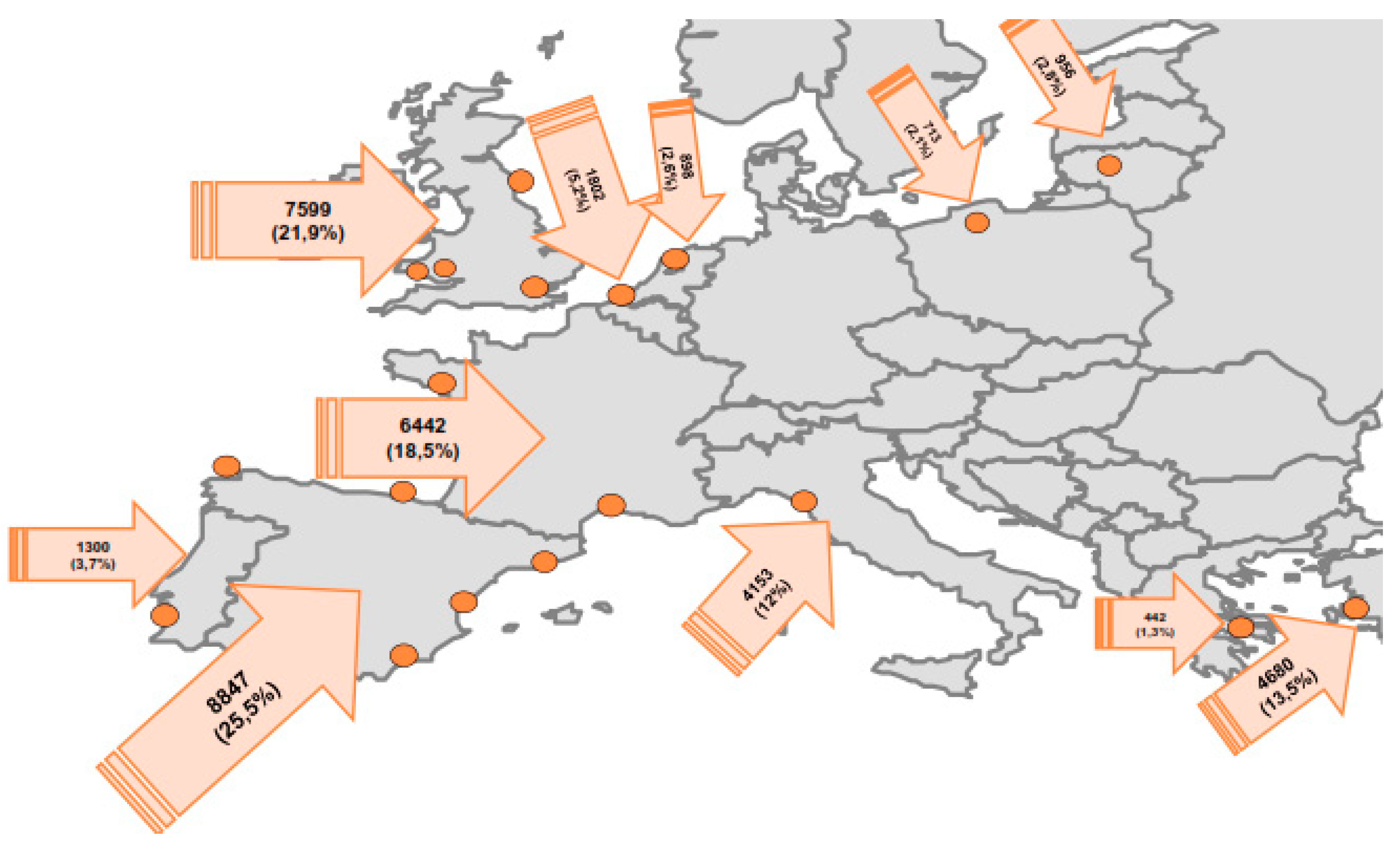
In this environment of different pricing dynamics, there are compelling reasons to rely on Spain’s gas import prices as an ideal reference to assess relationships between crude oil and long-term gas globally. Firstly, the characteristics of Spanish gas traders’ portfolio with a majority of long-term contracts indexed to oil and oil products similarly to Asia Pacific natural gas importers [1,2,5]. Secondly, since Spain imports most of the gas it consumes, a key factor that also influences gas prices in Spain is the importance of Liquefied Natural Gas (LNG) in gas procurement. In this sense, the ability to arbitrate in the global LNG market, makes the Spanish gas importer dynamically interconnected with other LNG markets, this influence resulting in higher exposure. Thirdly, the fact that Spain is the largest LNG importer in Europe (see Figure 1), reveals a similar gas trade pattern to other large LNG importers, especially in Asia. In this respect, it is important to note that the percentage of LNG over total gas imported in Asia Pacific, i.e., about 49%, is very close to that of Spain, i.e., about 42% (2015). In this regard, regulatory provisions to promote competition are more advanced than in many other countries and Spain has access to diverse, competing sources of gas. From a corporate perspective, in marked contrast to most of Continental Europe, there are credible competitors to the incumbent Gas Natural Fenosa, now Naturgy (such as Endesa, Iberdrola, BP, Shell and CEPSA), partly owing to the competitive long-term contracting practices of Spanish gas operators. It should be mentioned, however, that legacy from contract terms embedded in those long-term contracts such as take-or-pay (ToP) (a ToP obligation entails an unconditional obligation for payment, which enables the purchaser to get up to a certain threshold quantity of gas) clauses, may limit market liberalization as ToP obligations not only create problems in implementing third party access to transport infrastructures, but may introduce incentives for firms to avoid competition for end-users.
Within this context, further research into the current relationship between oil and long-term gas contract prices seems especially desirable at times when stable oil-gas relative pricing is under pressure in Asia and Europe [2,6]. As a matter of fact although both gas and oil prices should not deviate from pursuing common paths based on the oil-indexation hypothesis, the hypothesis is regularly challenged as gas markets develop into more liquid trading environments. As can be inferred, gaining more in-depth knowledge about price relationships between the two energy sources will definitely improve the transparency of natural gas markets dynamics and at the same time enhance short-term price forecasting and risk management, subjects of much interest for regulators and market players. In this sense and in spite of the large amount of work analysing volatility of crude oil prices solely [7,8,9,10,11], work related to long-term gas prices fluctuations and potential for an appropriate assessment of liberalization measures in gas markets is scarcer. This paper attempts to fill this gap by answering three key questions: First, whether long-term gas prices and crude oil volatility stylized facts behave similarly using a comprehensive GARCH framework. Secondly, supported by the fact that oil prices are the determining factor behind long-term gas prices, to quantify the degree of variability exercised by oil prices that are reflected in the gas price, using the proven methodology in the field of finance. Thirdly, to advance in an analytical manner the degree of success in transforming national gas markets following broader liberalization efforts by the EU Commission. In line with this and to the best of our knowledge, this paper is the first that addresses a systematic review of long-term gas prices volatility in a quantitative manner and seeks to make it directly applicable to energy policy.
Although a broad range of econometric methods have been used to characterize energy commodity variables and related features, those methods can be generally grouped into three areas, mainly analysis of fundamental value (we refer here by fundamental analysis of a variable to methodology intended to measure its intrinsic value, by examining mainly quantitative factors), market dynamics and the business cycle. In this sense, to achieve our goals, strong focus has been given to econometric tools in the first and second areas described. With regards to fundamental analysis we concentrate on multivariate GARCH models whereas to investigate into gas and oil market dynamics, the analysing volatility aspects seems most relevant to our aspirations (aside from volatility features, other commodity prices characteristics such as spillover effects, cross-asset linkages, common risk factors or even momentum features may be used for this purpose providing a different approach). In this sense, our approach is not limited to a single framework and therefore it benefits from qualified comparability of results.
Thus, this paper makes three main contributions: (i) it measures the extent to which crude oil volatility is displayed in long-term gas prices to provide reference information for the countries and regions where a majority of long-term gas contracts are oil-indexed. In this sense we anticipate that in spite of long-tern similarities between natural gas and oil prices evolution, medium-term interaction will be determined by volatility parametrization over the reference period 2002–2016; (ii) it unravels the nature of long-term gas supply effects facilitating a more precise assessment of the degree of liberalization of national gas pricing structures away from oil price indexation and (iii) it improves substantially clarity and understanding regarding the assessment of the level of transparency and competition, being these matters of great interest to both policymakers and gas market agents.
Overall, results from our research will provide a sound platform to improve understanding and at the same time explaining the development of traditional gas importing markets towards liberalization, questions followed by great interest by regulators and traders.
2. Results
2.1. Volatility Clustering and Nonlinear Autocorrelation
As discussed before and based on the impressive amount of information obtained over the last decade from financial markets and global commodities, researchers tend to agree on a few but extremely representative set of stylized features, also applicable to crude oil markets. Interest on such characteristics like heavy tails in asset return distributions, persistence, volatility clustering or autocorrelation of squared oil returns are not purely academic but also associated with processes leading to improve forecasting uncertainty. It is worth noting that two of these features are generally found to be more relevant than others as regards to the characterization of volatility conditions. Firstly, shocks to the variance of returns and changes in conditional volatility that generally persist rather than die down suggesting inherited persistence effects. Secondly, and in addition to persistence, the fact that large fluctuations seem to cluster together, reveals itself as one of the underlying elements which helps to begin to understand how volatility is affected by past realizations.
2.2. The Model
Empirical findings in the literature and experience in long-term gas contracting overwhelmingly support the fact that oil-driven stylized facts are also present in gas time series. Some of them appear to have more direct implications, i.e., skewness, kurtosis, and heavy-tailed distributions but others are more complex and difficult to trace like those affecting volatility of returns. In this section, we aim to characterize a sound volatility modelling tool for gas returns able to capture the above stylized facts prior to analyzing differences and similarities with other GARCH-type analysis of oil prices dynamics. It should be noted at this point that heteroskedastic models are of special relevance for volatility measuring not only because of the many applications in the econometric and financial domains but also because of the efficiency in parameter estimation. As it is described below, judgments about the appropriateness of GARCH-type models indicate a high degree of accuracy regarding the quality of forecasting. Nonetheless, the share nature of volatility that needs to be measured over a period, incorporates a certain degree of difficulty when comparing the volatility given by the models with the true volatility against which forecasting performance is measured.
There is a wide variety of studies addressing the performance of crude oil volatility but there is only a limited investigation into long-term gas contracts prices characteristics. In the literature of crude oil modelling, the Generalized Autoregressive Conditional Heteroscedastic (GARCH) and Stochastic Volatility (SV) models have been widely applied to improve understanding of the stochastic process beneath crude oil prices [8,9,10,12,13,14,15,16,17,18]. Moreover, the autoregressive VAR, TVAR, VEC, VEC-GARCH, and DCC-GARCH framework has been widely applied to investigate spillover effects [4,19,20]. In addition, other specific modelling approaches like Markov regime switching (MRS) model, support vector machine (SVM), wavelet technique and a variety of hybrid methods combining the methods mentioned before have also been used [21,22,23,24,25,26]. Possibly and in a category of its own the use of computational insight systems to examine the complexity embedded in oil prices has increased steadily in recent years [21,27,28,29,30]. These computational intelligence systems incorporate artificial neural network, genetic networks, expert systems or hybrid intelligent systems. Finally, limited research related to specific applications is also available, i.e., dynamic detection of fluctuation patterns [31] or hybrid models incorporating financial variables [32]. In summary, while crude oil markets form a complex system including non-linearities, multi-factor dimensions and are subject to the impact of structural breaks, forecasting methods are constantly emerging, and performance has been continuously improving.
The common strand in GARCH-type representations allowing a finite, time-varying second moment distribution of returns, addresses directly volatility clustering in the data and mitigates the problem of fat tails. Within this field, it is difficult, however, to identify a model that consistently dominates the other since model superiority is typically assessed with regard to both the flexibility in capturing the stylized facts in which we concentrate, but also as regards to its ability to forecast [9]. There are ample studies addressing the accuracy of crude oil volatility modeling. Reference [7] for instance finds that the GJR model fits well for heating oil and natural gas volatilities, whereas the standard GARCH model fits better for crude oil and unleaded gasoline volatilities. Narayan and Narayan [12] favor the use of the EGARCH model, whereas Kang and Yoon [8] conclude that the CGARCH and FIGARCH models are better to capture persistence in the volatility of crude oil prices. In contrast with this, Mohammadi and Su [13] compared the forecasting accuracy of four GARCH models to suggest that conditional volatility of oil returns dissipate at an exponential rate as in the GARCH models rather than at a slow hyperbolic rate implied by the FIGARCH model. Wei et al. [14] also conclude that none of the GARCH-class models, including the FIGARCH one, outperforms the others in all situations although non-linear models like EGARCH or GJR-GARCH exhibit greater forecasting accuracy. More recently, Wang et al. [21] reveal that the multivariate GARCH model has better performance than the univariate GARCH model overall.
Modelling Spanish gas (SG) returns volatility is performed in two steps. The first step involves determining the specification of the GARCH (p, q) model for conditional volatility and its diagnostic tests. Secondly, we analyze asymmetric effects through extended GARCH models. As regards the first point the evidence gathered in the empirical literature on oil price volatility modeling tends to support the view that GARCH models seem to work well in most applied situations in spite that there is potential for improvement through alternative methods [17]. However, to model volatility, and from experience in oil markets (evidence has been found for oil returns that ‘bad news’ have a greater capacity to generate high volatility than ‘good news’), it is necessary to test the leverage effect of SG returns. In line with this, three different volatility model specifications—GARCH, EGARCH, and GJR-GARCH—are considered in the research.
Following standard practice in the literature, model estimation is based on the maximum-likelihood principle once a distribution for the innovations, εt has been specified. Although we proceed from the assumption that the innovations are Gaussian, we also verify that a t-distribution does not characterize the distribution of the returns better than the Gaussian distribution regarding volatility behavior. In model selection, three indicators, i.e., the log-likelihood, the Akaike information (AIC) and the Bayesian information criteria (BIC) are used to evaluate the most appropriate models over alternative GARCH-type (p, q) models by varying p and q parameters from 0 to 3. As can be seen in Table 1, EGARCH shows superior results (largest log-likelihood and smallest AIC) to the rest. However, the GARCH (1, 1) was superior in BIC as this criterion imposes additional penalties for additional estimated parameters. This outcome is acceptable since EGARCH provides the richest range of parametrization to capture the stylized facts such as volatility clustering, leverage effect and long-memory in the volatility. We select within each class EGARCH (2, 1) as it has lower AIC, GARCH (1, 1) and GJR-GARCH (1, 1) for detailed diagnostics.
Table 2 presents the in-sample estimation results for the different volatility models discussed. The lower part of Table 2 shows some of the results of the diagnostic test on standardized residuals, i.e., a Q test on squared standardized residuals, an ARCH test, and a Jarque–Bera test. The results reported for Ljung-Box Q and the Engle’s Arch tests clearly confirm that the three models reproduce ARCH effects in an appropriate manner revealing the absence of significant autocorrelation of εt2 at the 95% confidence level.
Concluding results from the detailed comparison of the three selected models lead us to favor the EGARCH (2, 1) model that not only shows the largest log-likelihood and the lowest AIC in spite of being penalized on an additional number of parameters but also incorporates some attractive features. First, it does not impose restrictions on any model parameters. Second, it includes a provision for oscillatory behavior in the conditional variance and at the same time indicating whether shocks to the variance are persistent or not. Third, the EGARCH model allows evaluation of asymmetric volatility effects. Assuming and the selected EGARCH (2, 1) model reads as follows:
It is interesting to note that the resulting EGARCH model could slightly improve the widely used GARCH specification when modeling oil returns as evidenced by studies favoring nonlinear GARCH-class models [12,14]. More importantly and as seen in Table 2 estimates for ARCH and GARCH parameters are statistically significant especially for the EGARCH (2, 1) model what leads us to conclude that this specification is the more robust. Analysing further resulting parameters, we have the following results regarding two main features of price volatility, namely asymmetry, and persistence of shocks.
- (1)
- ARCH effects. The model shows a positive and significant ARCH parameter with a value of 0.253. This confirms the fact that larger shocks increase SG returns volatility, regardless of their signs, to a greater extent than smaller shocks. The magnitude of the effect is measured by the term determining the size of the new innovation into the series.
- (2)
- GARCH effects. These are determined by GARCH coefficients commonly named βi, i.e., those determining the influence of the past conditional volatilities on the current conditional variance. In our case since |Σ βi| ˂ 1 (|β|˂ 1 shows that the necessary stationary condition is met and establishes the conditions for covariance stationarity of the EGARCH model under particular specifications of the error distribution.) and the EGARCH model is always stationary (if εt has a Normal Distribution). Moreover, all ARCH and GARCH parameters are highly significant whereas the leverage coefficient is not. Persistence (determined by |Σ βi|) is lower than one reflecting no restrictions in the second moment although its value of 0.802 is not far from the nonstationarity boundary allowed by EGARCH models. Results of the Ljung-Box and ARCH tests on returns and residuals square respectively, using standardized innovations of the estimated model, indicate acceptance (h = 0 with highly significant p-values) of their respective null hypotheses and confirm the validity of the selected EGARCH model. Based on the above mentioned, it is reasonable to state that volatility of SG returns is genuinely persistent, with the estimated |Σ βi|) parameter controlling the decay of the autocorrelation function. Another parameter widely used to measure volatility persistence is the half-life of a volatility shock (HLS), i.e., the time it takes for the volatility to move halfway through its unconditional variance after the shock is perceived. HLS can be measured as: HLS = Ln 0.5/Ln β [33]. In our case, and to be able to compare the results with existing literature on oil price volatility persistence, we consider the β value from our EGARCH (1, 1) specification of 0.781 implying HLS of about 2.8 months or approximately 85 days. Interestingly, the evidence found for high volatility persistence in the Brent market of HLS about 87 days [14], 95 days [12] or even 128 days [13] using also EGARCH (1, 1) specifications for Brent returns reflects the high level of persistence inherited by long-term gas prices from Brent. Moreover, it can be observed that in spite of the fact that volatility persistence is inherently unobservable, it is transmitted effectively through the oil-indexation mechanism.
- (3)
- Asymmetric leverage. Reported results for the asymmetric leverage coefficients show consistent effects: the EGARCH coefficient is positive in agreement with negative coefficients found in all the GJR-GARCH models analyzed, this indicating that positive shocks would increase volatility more than negative shocks. However, none of the leverage parameters in the variance equation are significant at either 5% or 10% levels indicating that evidence of asymmetric response to good and bad news appears mixed in line with results found in literature for Brent returns [13,34,35] and in spite of asymmetry coefficient found significant in other research also using EGARCH models [14]. The potential for positive leverage effects is somehow unexpected as it is in contradiction with negative asymmetric leverage effects sometimes reported for the Brent market, i.e., downward movements (shocks) that raise oil prices are more often followed by greater volatilities than upward movements of the same magnitude that reduce the oil price [12]. In our case, the small value of the leverage coefficients and the fact that parameters are always non-significant would lead to rejecting the hypothesis of asymmetry effects on conditional volatility overall. These results would reinforce the idea of mixed effects found in the literature for asymmetric effects in oil prices.
2.3. Quantitative Evaluation of Volatility Clustering
Among all the properties analyzed before, the phenomenon of volatility clustering has intrigued many researchers and oriented in a major way the development of stochastic models in financial forecasting and derivatives pricing. Observation of this feature in financial time series has led primarily to the use of GARCH models as in essence these models are able to reflect the fact that fluctuations in the current period will impact on expected fluctuations in the future. However, quantification of volatility clustering effects using autoregressive heteroskedastic models is not generally sufficient since this property is not intrinsically linked to a GARCH specification and other methodologies such as the analysis of autocorrelation of absolute returns [36], the copula approach [37] or even factor models for log volatilities [38] have been developed. Following this line of work, not necessarily linked to ARCH-type modelling and also specific research based on rolling analysis of financial time series (in our case we use rolling analysis to assess scale of volatility clustering effects a methodology that reveals itself to be ideal for the proposed analysis within selected border zones) [39,40,41,42] we introduce an index (Rn) as a quantitative measure of volatility clustering that can be used to compare the degree of volatility clustering along SG and Brent time series. This index is calculated over a rolling window of reference to obtain valid estimates of volatility clustering stability. The process is simple: we begin by putting a window on the first month of the whole series and count the number of months over a p% threshold fluctuation within an n-month window. We then move on to the second month of the whole series and again count the number of months over the p% threshold fluctuations within this next n-month window. We repeat the same procedure until we finish scanning through the whole-time series. Finally, we calculate the ratio Rn, mathematically defined as Rn = σe/σG, where σe and σG are the standard deviation of the number of days of the largest (1 − p)% fluctuations within an n-month period for the empirical and for the simulated Gaussian datasets respectively. The larger the ratio, the larger the degree of clustering is. As a preliminary step to selecting the best size of the rolling window, a detailed analysis reveals that window size of 20 months delivers maximum visibility of clustering effects over a wider range of p% largest fluctuations. Moreover, for different time periods considered, the relationship between crude oil and gas prices established by the Rn index is a unique parameter connecting crude oil and gas price volatility clustering characteristics.
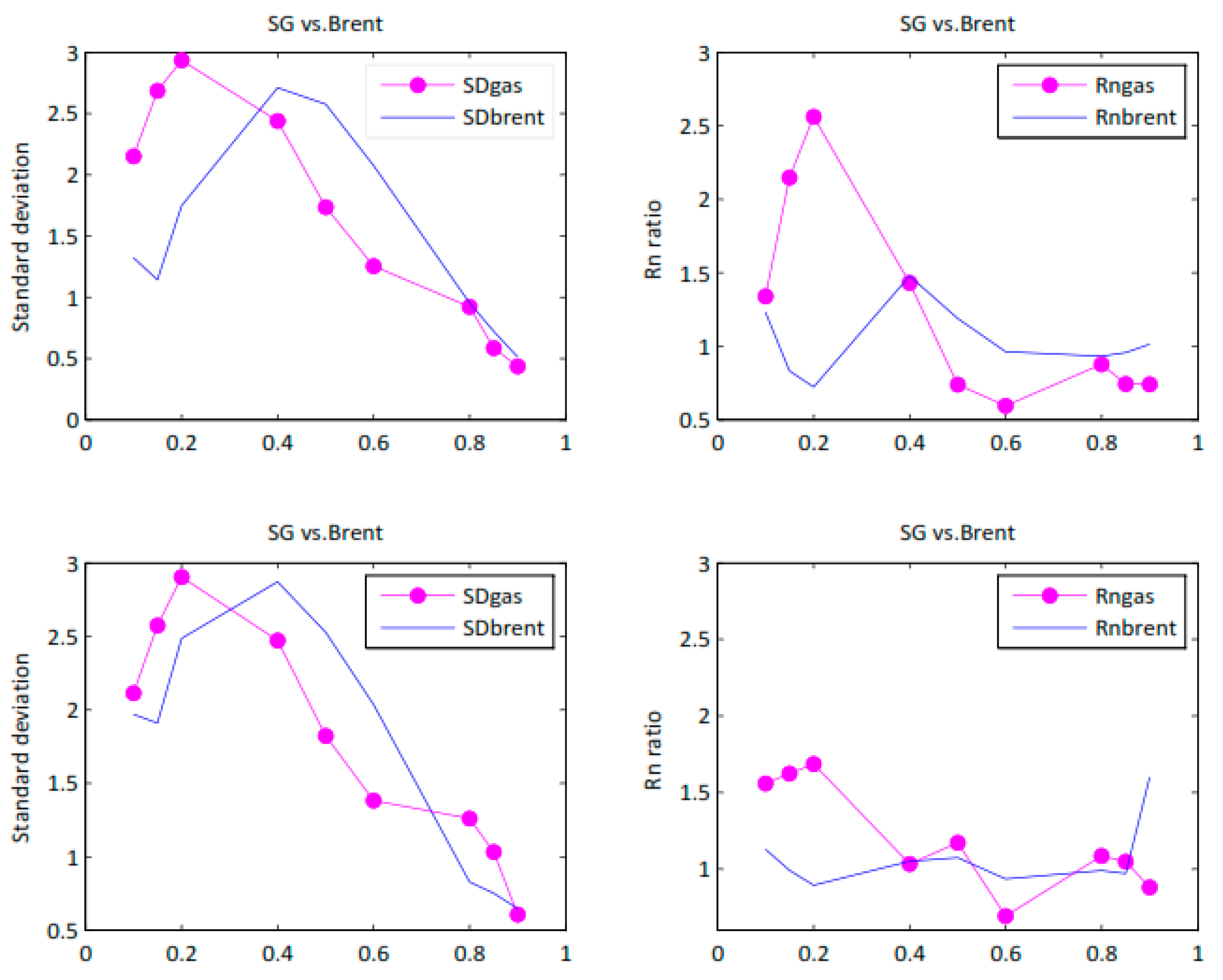
Figure 2 shows the different p% threshold options (expressed as a rate over one), how standard deviation (SD) and Rn vary from one period to another. Two different periods to be covered by our investigation are identified. The first period, i.e., 2002–2013 (top row) mainly characterized by the credit crunch in 2008 and the second period extended until 2016 (bottom row) to include the collapse of oil prices since late 2014 and the current oversupply situation.
It is apparent from Figure 2 that for SG returns p = 20% shows the highest Rn values (implying maximum clustering visibility) whereas Brent returns show maximum Rn values at about p = 40% for both periods. Certainly, most relevant to our investigation is the fact that when taking into account the 10% largest fluctuations (p = 90%), Rn values for Brent returns are consistently higher than for SG returns, indicating that SG prices do not reflect entirely Brent volatility clustering dimension, as it was to be expected from effects from other factors embedded into gas prices.
Examining the results more closely, we can evaluate how clusters of volatility evolve incrementally. A simple calculation shows that the increase in the clustering index Rn between the first and the second study periods is about 19% for gas whereas for Brent is about 58%, always considering the p = 90% threshold. Consequently, it can be said that the amount of volatility effectively reflected by SG gas is only about a 33% of the total, thus resulting in the diminished influence of oil price indexations since 2013 until 2016.
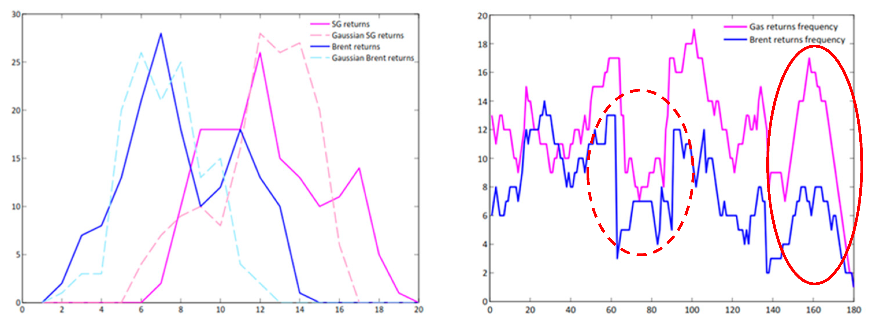
In order to expand our investigation to effectively advance patterns of behavior for clustering in both series, we simply compare results obtained for p = 20% (SG) and p = 40% (Brent), with those obtained with a similar random Gaussian series (see the left chart in Figure 3).
As it can be seen, both SG returns and Brent returns (solid) display a broader spread of occurrence over the threshold than corresponding normally distributed returns (dash) implying an Rn higher than one in each case.
Figure 3 (right) shows that when plotting Brent vs. SG returns clustering behavior, SG clustering pattern although rather similar, seems to be lagging behind crude oil within a band of 3 to 6 months (solid circle) as it would be expected from the lagging effects in the gas price formula. Interestingly, the scale of volatility clustering variation is very similar on average in spite of sporadic opposite effects (dash circle), possibly reflecting balancing of traders’ portfolios on an occasional basis.
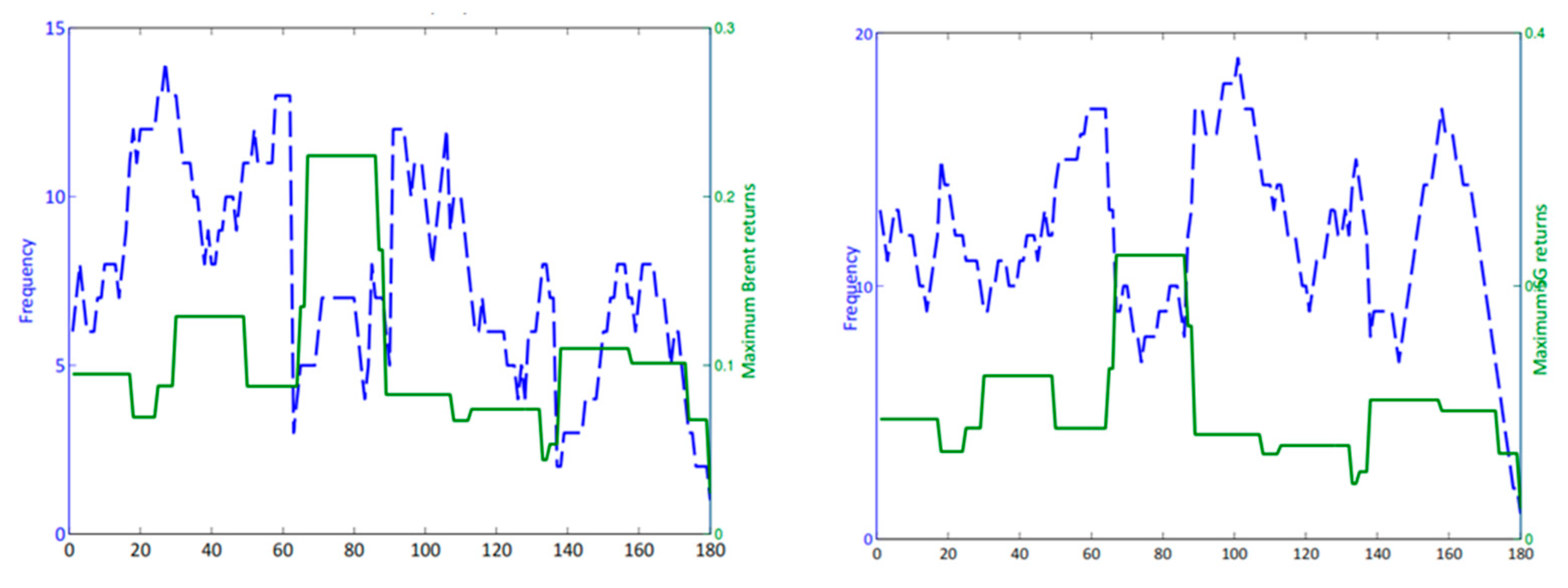
Figure 4 below represents standard absolute crude oil and SG returns series against clustering dimension, i.e., number of peaks over 40% and 20% threshold respectively.
As it can be seen, bumps shaping volatility clustering from the analysis (dash) tend to be aligned with heights and valleys in returns (solid) this being an indication that volatility clustering is intimately related with largest and smallest changes over the time series. Moreover, a manifestation of maximum volatility clustering effects coincides with a sharp decrease in returns in 2008.
2.4. Qualitative Assessment of Oil-Indexed Effects into Gas Market Dynamics
Although expectations for gas markets in Europe to replace oil indexation with liquid traded benchmarks have been high over the last decades, these expectations very much inspired by the success of United Kingdom gas market developments, replacement of the traditional long-term oil-indexed bilateral contracts by a gas hub-based model has been limited. In this regard, the existing literature on market liberalization development has been prescriptive, focusing on policy recommendations but paying less attention to the main drivers that have contributed to the inertia brought about by the existing contractual set-up in European imports. Moreover, while the oil-indexation model has been criticized since the 1990’s, the causes for their persistence are only passingly explained as the interests of companies are rather ignored [43]. Moreover, whereas analytical research to unveil gas pricing evolution is scarce, it is noticed that the UK’s gas pricing arrangements differ significantly from those of Continental Europe [44]. The legislator, the EU Commission although having successfully provided open access for third parties to monopolistic gas infrastructure in most of the EU nations, remains limited in regard to policies and directives related with gas sourcing issues, as this would interfere with legacy gas supply agreements well into the 2020s, and in some cases the 2030s. The fact that some of the key producers like Gazprom, Sonatrach or other several LNG exporting countries, prefer long-term bilateral contracting results in oil-indexation playing still a very relevant role in the future. Last but not least, in spite of the fact that upstream producers are forced to increasingly incorporate gas hub price elements in their long-term contracts price indexation formulas, they have an incentive also to actively trade on hubs in the hope of influencing price formation as this affects their bilateral long-term contracts [45]. In this market environment, exploring the resilience of crude oil prices to changes in regional gas markets in a dynamic manner is very relevant. The volatility clustering decomposition method provides an analytical basis necessary to support further evidence about the contribution of crude oil prices to regional natural gas price returns. Although we will not discuss the economic mechanisms which have been proposed to explain the origin of this volatility clustering, the assessment of the results of the previous sections sheds light on certain areas of interest: Firstly, according to the values of the Rn index, which is the component that measures the resulting fraction in the natural gas price returns explained by crude oil returns, the contribution of Brent price volatility to the SG price returns has decreased since 2013 until 2016. This could be an indication that gas supply contracting strategies of Spanish traders may have evolved towards a more spot and short-term focus as contract prices have fallen due to upcoming oversupply over the same period.
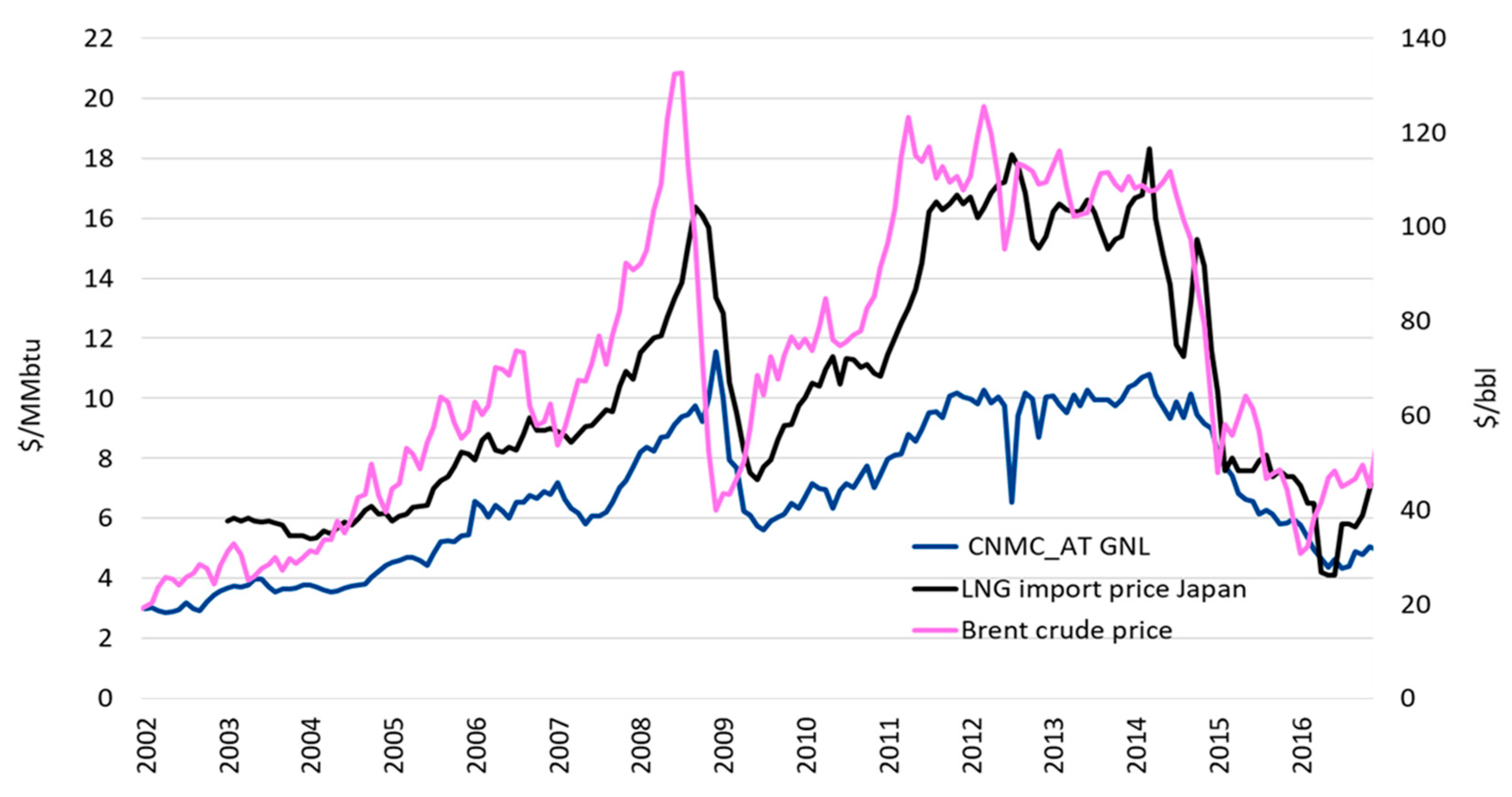
Figure 5 illustrates how since late 2012 while oil prices decrease, gas prices typically linked to oil or oil products follow suit.
Secondly, the influence of open market references such as Henry Hub into Europe continues to be very limited and the North American shale revolution has had little impact even on NBP prices [46,47]. The fact that most of the integrated gas suppliers would still be eager to retain commodity price risk and upside in line with traditional business models, is very much at the heart of this results. Furthermore, and although between 2011 and 2014, many LNG buyers have wanted to secure some Henry Hub indexation to diversify exposure to oil, new projects fostering more Henry Hub indexation feeding into Continental Europe, pricing arrangements may be constrained (pricing terms to be offered but also the uncertain timing that new volumes face are relevant in that respect). Our research contributes, to better understand, in this respect that market-based factors such as LNG spot and medium-term supply alternatives are key drivers for the diminished influence of oil-indexed structures since 2013 and until 2016. Thirdly, in regard to volatility patterns analysis, Figure 3 illustrates how oil and gas share some similar characteristics and especially how gas prices reveal very clearly the lagging effects in volatility clustering resulting from the lagging effects in the oil-indexed gas price formula. As discussed previously, this analysis of clustering patterns reveals that sporadically Spanish traders are able to balance their portfolios through traded hub supply with volatility clustering patterns being disrupted when compared with oil prices. In this regard, our methodology allows for an in-depth diagnosis of the evolution of gas portfolios in Spain showing the extent to which the use of market-based approaches has resulted in significant effects away from oil-indexation influence.
It has to be noted that results from the volatility clustering analysis shown above are difficult to compare with previous studies given the newly applied methodology in our research. However, as the comments above show, quantification of volatility clustering effects from oil prices into gas prices opens an interesting perspective to better understand timely effects of oil prices relative to other variables in the equation.
3. Discussion
In this paper, we investigate into the intrinsic relationship between oil prices and long-term gas contract prices using a novel approach to provide appropriate information and quantify the level of influence reached by oil prices into gas prices. Consequently, we provide a tool to facilitate a sound understanding of gas hub expansion and underlying gas market implications.
In the first place, we analyze stylized facts of long-term gas prices characterizing the model that best fit our reality to conclude on the EGARCH (2, 1) class as the optimum fit. As a result, we find conditional volatility of gas prices to be modestly persistent, with a volatility half-life of about 85 days against evidence found for higher volatility persistence in the Brent market up to 125 days. These results show that when comparing persistence of SG returns to that of oil returns, this extensively studied in the last decades, we note that although gas returns persistence remains at the lower end of the spectrum, it still reflects a high level of persistence overall. Moreover, the legacy of Brent oil is clearly observed in gas prices in spite of the fact that volatility persistence is inherently unobservable. Supported by modeling results, we propose a novel approach to quantify volatility clustering characteristics of crude oil prices against those of long-term gas prices. In order to measure the extent of the impact, we introduce an index, i.e., Rn, which allows to evaluate and compare volatility clustering effects incrementally over a rolling window through the sample. In the light of these results, it can be clearly seen that patterns of gas price clustering relative to crude oil prices is not necessarily identical and in fact there is diminished influence of oil price indexations since 2013 until 2016. This shows that Spanish gas prices do not reflect entirely Brent volatility clustering dimension, as it was to be expected from effects from other factors embedded into gas prices. Finally, we found that the analysis of gas volatility clustering dynamics since 2002 versus gas market conditions over the period, does also support the fact that sporadic supplies, being integrated into the portfolio of Spanish traders on an opportunistic basis, are those leading to disrupted patterns from those of oil prices.
Results from our investigation have significant implications for economic analysis and policy-making decisions. Broadly speaking, the novel analysis performed provides a quantitative benchmark to assess oil price influence on gas price structures and in turn, it reveals the degree of penetration of other price mechanisms rather than oil-indexed in an objective manner. In this sense, our research provides quantitative tools to better understand that market-based approaches such as spot and medium-term supply alternatives seem to be a key driver for success in transforming gas markets following a broader privatization and liberalization paradigm. Furthermore, and in the absence of similar research done in the past, it is expected that the new perspective that is opening up within this framework will motivate new research to expand the scope of investigation.
Given the importance of oil-indexed contract structures in understanding the degree of penetration of liquid hub pricing, regular updates on the size of the effects observed should facilitate a precise assessment of the degree of liberalization of national gas markets and improve the level of transparency, these matters of great interest to both policymakers and gas market agents. Finally, it can be suggested that the traditional well-diversified portfolio of natural gas imports in Spain needs to be maintained in order to reduce the excessive risk brought by the shock of crude oil price fluctuations.
4. Material and Methods
Many empirical studies have investigated on the long-term relationship between natural gas and oil prices, mostly in the US and the UK, by large the most liquid markets worldwide and therefore showing a less evident connection than gas markets in Continental Europe or Japan.
Special attention has been devoted in the past to the degree of integration between natural gas and oil markets with a focus on whether a separation between the two types of prices was [48,49]. In the US, research has found that oil and gas series are generally cointegrated with strong evidence for a regime-switching connection between natural gas and oil price [50]. More recently [51,52] deal very accurately with the cointegrating relationship between natural gas and crude oil to find further evidence that both prices do not permanently ‘decouple’ but rather experience a temporary shift in regimes but also that the so called shale gas revolution has affected the relationship across both variables although it is not possible to assess whether or not a new long-run relationship between oil and gas has been established.
In the UK, studies like [3] indicate that the UK energy market is highly integrated with oil prices leading gas prices and that UK gas prices tend to decouple during fall and early winter, when they increase relative to oil consistent with seasonal demand for natural gas creating gas-specific pricing. Moreover, ref [53] show that European spot markets do also follow the same determination process as in the UK. Interestingly, [4] using panel cointegration analysis conclude that oil price volatility has a negative impact on gas price. The shock impact is weak in North America, lags in Europe and is most significant in Asia. In addition, they find that the response of natural gas import prices to increases and decreases in international crude oil prices shows an asymmetrical mechanism, of which the decreasing impact is relatively stronger. The hypothesis that Brent oil prices play a leading role in European and Japanese gas price fluctuations is reiterated in research from [19] using a VEC-MGARCH approach. As a very relevant finding to this investigation, they confirm that volatility in the oil market spillovers onto natural gas but not backward, this applies to both the US and European energy markets.
It has to be noted that in recent years, the nature of the non-linear relationships between crude oil prices and regional natural gas prices has led to increased interest in multi-scale modeling approaches interconnecting several gas markets simultaneously. In this regard, empirical mode decomposition techniques (EMD) are increasingly being used to capture the different fluctuation features of the original series at different scales. Using EMD and cross-correlation method, [54] confirm once more that oil prices play the leading role in affecting Asian and European natural gas prices, having advance effects of one to three months and one to six months, respectively. Interestingly, [46] using EMD and the VAR model unveil that the effects of oil price shocks on the European gas market have become stronger since the shale gas revolution.
In view of this evidence, the first step toward understanding the cause behind crude oil effects seems most relevant to our case. Not surprisingly, and since oil is one of the most important drivers in the economy, with an intriguing connection with other factors like inflation, stocks, bonds and economic growth, the amount of research on the relationship between oil price volatility and other aspects has been fluent and especially intense over the last few years in fields like macroeconomy and exchange rates [55,56,57,58,59,60] or stock markets [61,62,63]. In a category of its own, a fewer number of studies approach crude oil price and returns in relation to other commodities also including natural gas [64,65,66,67,68,69]. Finally, and as for other traded commodities, a highly sophisticated category of research is available on both volatility modelling and forecasting evaluation [8,9,10,11,12,13,14,15,21,70,71,72,73], both perhaps the most relevant areas for our research.
It becomes especially important in the context of this study, the concept of persistence and the notion of memory properties of time series, i.e., to what extent the effect of an infinitesimally small shock in the price series will be influencing the future predictions for a long time. Although persistence on the mean has been investigated in depth for oil prices series [74] the existing literature is far from a consensus on its unit root properties in spite of the fact that generic tests are mostly unable to reject non-stationarity of the crude oil prices meaning that oil prices are consistent with there being a unit root.
Of all the factors involved in determining the term structure of crude oil prices, the effects of structural breaks is the most challenging. According to [16,75], the inclusion of information regarding structural changes reduces volatility persistence and improves the understanding of volatility transmission in crude oil markets.
Author Contributions
For research articles with several authors, a short paragraph specifying their individual contributions must be provided. The following statements should be used “Conceptualization, P.C.-B. and C.R.-M.; Methodology, P.C.-B.; Software, P.C.-B.; Validation, P.C.-B. and C.R.-M., Formal Analysis, P.C.-B.; Investigation, P.C.-B. and C.R.-M.; Resources, P.C.-B. and C.R.-M.; Data Curation, P.C.-B.; Writing-Original Draft Preparation, P.C.-B.; Writing-Review & Editing, C.R.-M.; Visualization, P.C.-B.; Supervision, C.R.-M.; Project Administration, P.C.-B.; Funding Acquisition, None.
Funding
This research received no external funding.
Conflicts of Interest
The authors declare no conflict of interest.
Appendix A
ARCH Models
ARCH models develop a theoretical framework to simulate variance clustering in the residuals of a stochastic variable implying nonlinear dependence among the squared errors of the first moment model. A generic ARCH model [76] follows a process as below:
where . Assuming ,
Equation (A2) can also be written as an AR (m) model as below:
where is a white noise process.
GARCH Models
Bollerslev [68] expands on [77] original work by allowing the conditional variance to follow an ARMA process. A GARCH (r, m) model can be written as:
where and |Σ | ˂ 1.
The latter constraint on ensures that the unconditional variance of is finite, even though its conditional variance evolves over time.
ASYMMETRIC GARCH Models
A major assumption embedded into ARCH/GARCH modeling is that positive and negative shocks have the same effect on volatility. In practice, the price of stochastic time series reacts differently to lower or higher impulses causing what is called a leverage effects. Asymmetric GARCH models are designed to capture leverage effects.
The asymmetric GARCH models discussed in the article include GJR-GARCH [78] and exponential GARCH (EGARCH) models [33].
Glosten, Jagannathan, and Runkle [78] develop an additional parameter called as a threshold to determine the leverage effect. A GJR-GARCH (1, 1) model can be generally expressed as:
where if and if
Similarly, Nelson [33] develops a GARCH (EGARCH) model that ensures that all the estimated coefficients are positive and therefore does not require non-negativity constrains.
The EGARCH (r, m) model in simplified form is:
References
- International Energy Agency. Available online: https://www.iea.org/publications/freepublications/publication/partner-country-series-developing-a-natural-gas-trading-hub-in-asia.html (accessed on 23 December 2017).
- Aguilera, R.F.; Inchauspe, J.; Ripple, R.D. The Asia Pacific natural gas market: Large enough for all? Energy Policy 2014, 65, 1–6. [Google Scholar] [CrossRef]
- Asche, F.; Oglend, A.; Osmundsen, P. Modeling UK Natural Gas Prices when Gas Prices Periodically Decouple from the Oil Price. Energy J. 2017, 38, 1. [Google Scholar] [CrossRef]
- Ji, Q.; Geng, J.B.; Fan, Y. Separated influence of crude oil prices on regional natural gas import prices. Energy Policy 2014, 70, 96–105. [Google Scholar] [CrossRef]
- IGU (International Gas Union). Wholesale Gas Price Survey; IGU: Barcelona, Spain, 2016. [Google Scholar]
- Erdos, P. Have oil and gas prices got separated? Energy Policy 2012, 49, 707–718. [Google Scholar] [CrossRef]
- Sadorsky, P. Modelling and forecasting petroleum futures volatility. Energy Econ. 2006, 28, 467–488. [Google Scholar] [CrossRef]
- Kang, S.; Yoon, S. Forecasting Volatility of Crude Oil Markets. Energy Econ. 2009, 31, 119–125. [Google Scholar] [CrossRef]
- Cheung, C. Modelling and forecasting crude oil markets using ARCH-type models. Energy Policy 2009, 37, 2346–2355. [Google Scholar] [CrossRef]
- Sevi, B. Forecasting the volatility of crude oil futures using intraday data. Eur. J. Oper. Res. 2014, 235, 643–659. [Google Scholar] [CrossRef]
- Serletis, A.; Xu, L. Volatility and a century of energy markets dynamics. Energy Econ. 2016, 55, 1–9. [Google Scholar] [CrossRef]
- Narayan, P.; Narayan, S. Modelling Oil Price Volatility. Energy Policy 2007, 35, 6549–6553. [Google Scholar] [CrossRef]
- Mohammadi, H.; Su, L. International Evidence on Crude Oil Price Dynamics: Applications of ARIMA-GARCH Models. Energy Econ. 2010, 32, 1001–1008. [Google Scholar] [CrossRef]
- Wei, Y.; Wang, Y.; Huang, D. Forecasting crude oil market volatility using GARCH models. Energy Econ. 2010, 32, 1477–1484. [Google Scholar] [CrossRef]
- Lux, T.; Segnon, M.; Gupta, R. Forecasting crude oil price volatility and value-at-risk: Evidence from historical and recent data. Energy Econ. 2016, 56, 117–133. [Google Scholar] [CrossRef] [Green Version]
- Kang, S.H.; Cheong, C.; Yoon, S.M. Structural changes and volatility transmission in crude oil. Phys. A 2011, 390, 4317–4324. [Google Scholar] [CrossRef]
- Hou, A.; Suardi, S. A non-parametric GARCH model of crude oil price return volatility. Energy Econ. 2012, 24, 618–626. [Google Scholar] [CrossRef]
- Dritsaki, C. The performance of hybrid ARIMA-GARCH modeling and forecasting oil price. Int. J. Energy Econ. Policy 2018, 8, 14–21. [Google Scholar]
- Lin, B.; Li, J. The spillover effects across natural gas and oil markets: Based on the VEC–MGARCH framework. Appl. Energy 2015, 15, 229–241. [Google Scholar] [CrossRef]
- Souza, A.; Righi, M.B.; Schlender, S.G.; Arruda, D. Investigating dynamic conditional correlation between crude oil and fuels in non-linear framework: The financial and economic role of structural breaks. Energy Econ. 2015, 49, 23–32. [Google Scholar]
- Wang, D.; Wu, C.; Yang, L. Forecasting crude oil market volatility: A Markov switching multifractal volatility approach. Int. J. For. 2016, 32, 1–9. [Google Scholar] [CrossRef]
- Fong, W.; See, K. Markov Switching Model of the Conditional Volatility of Crude Oil Futures Prices. Energy Econ. 2002, 24, 71–95. [Google Scholar] [CrossRef]
- Di Sanzo, S. A Markov switching long memory model of crude oil price return volatility. Energy Econ. 2018, 74, 351–359. [Google Scholar] [CrossRef]
- Zhang, Y.; Zhang, Y.; Zhang, L. Interpreting the crude oil price movements: Evidence from the regime switching model. Appl. Energy 2015, 143, 96–109. [Google Scholar] [CrossRef]
- Zhang, J.L.; Zhang, Y.J.; Zhang, L. A novel hybrid method for crude oil price forecasting. Energy Econ. 2015, 49, 649–659. [Google Scholar] [CrossRef]
- Zhang, Y.; Yao, T.; He, L.; Ripple, R. Volatility forecasting of crude oil market: Can the regime switching GARCH model beat the single-regime GARCH models? Int. Rev. Econ. Financ. 2019, 59, 302–317. [Google Scholar] [CrossRef]
- Chiroma, H.; Abdulkareem, S.; Herawan, T. Evolutionary neural network model for West Texas intermediate crude oil price prediction. Appl. Energy 2015, 142, 266–273. [Google Scholar] [CrossRef]
- Li, T.; Zhou, M.; Guo, C.; Luo, M.; Wu, J.; Pan, F. Forecasting crude oil price using EEMD and RVM with adaptive PSO-based kernels. Energies 2016, 9, 1014. [Google Scholar] [CrossRef]
- Yu, L.A.; Dai, W.; Tang, L. A novel decomposition ensemble model with extended extreme learning machine for crude oil price forecasting. Eng. Appl. Artif. Intell. 2016, 47, 110–121. [Google Scholar] [CrossRef]
- Chiroma, H.; Abdulkareem, S.; Noor, A.S.M.; Abubakar, A.I.; Safa, N.S.; Shuib, L. A review on artificial intelligence methodologies for the forecasting of crude oil price. Intell. Autom. Soft Comput. 2016, 22, 449–462. [Google Scholar] [CrossRef]
- Gao, X.; Fang, W.; An, F.; Wang, Y. Detecting method for crude oil price fluctuation mechanism under different periodic time series. Appl. Energy 2017, 192, 201–212. [Google Scholar] [CrossRef]
- Kristjanpoller, W.; Minutolo, M. Forecasting volatility of oil price using an artificial neural network-GARCH model. Expert Syst. Appl. 2016, 65, 233–241. [Google Scholar] [CrossRef]
- Nelson, D. Conditional heteroskedasticity in asset returns: A new approach. Econometrica 1991, 59, 347–370. [Google Scholar] [CrossRef]
- Yang, C.; Gong, X.; Zhang, H. Volatility forecasting of crude oil futures: The role of investor sentiment and leverage effect. Resour. Policy 2018. [Google Scholar] [CrossRef]
- Chen, L.; Zerilli, P.; Baum, C. Leverage effects and stochastic volatility in spot oil returns: A Bayesian approach with VaR and CVaR applications. Energy Econ. 2018. [Google Scholar] [CrossRef]
- Niu, H.; Wang, J. Volatility clustering and long memory of financial time series and financial price model. Digit. Signal Process. 2013, 23, 489–498. [Google Scholar] [CrossRef]
- Ning, C.; Xu, D.; Wirjanto, T. Is volatility clustering of asset returns asymmetric? J. Bank. Financ. 2015, 52, 62–76. [Google Scholar] [CrossRef]
- Verme, A. A Cluster Driven Log-Volatility Factor Model: A Deepening on the Source of the Volatility Clustering. Quant. Financ. 2018, 1–16. [Google Scholar] [CrossRef]
- Tseng, J.; Li, S. Quantifying volatility clustering in financial time series. Int. Rev. Financ. Anal. 2012, 23, 11–19. [Google Scholar] [CrossRef]
- Alexander, C. Market Models: A Guide to Financial Data Analysis; John Wiley & Sons: Chichester, UK, 2011. [Google Scholar]
- Dacorogna, M.; Genc, R.; Müller, U.; Olsen, R.; Pictet, O. An Introduction to High-Frequency Finance; Academic Press: San Diego, CA, USA, 2001. [Google Scholar]
- Zivot, E.; Wang, J. Modelling Financial Time Series; Springer: Berlin, Germany, 2006. [Google Scholar]
- Buhanist, P. Path Dependency in the Energy Industry: The Case of Long-term Oil-indexed Gas Import Contracts in Continental Europe. Int. J. Energy Econ. Policy 2015, 5, 934–948. [Google Scholar]
- Konoplyanik, A. Long-term investments in the gas industry: The role of oil indexation. In Proceedings of the Workshop on Contractual Issues Related to Energy Trade, Conference Organized Jointly by the Energy Charter Secretariat & Hungarian Ministry of National Development, Budapest, Hungary, 20 March 2013. [Google Scholar]
- ACER. 5th Annual Market Monitoring Report on Gas Wholesale Markets. Available online: http://www.acer.europa.eu/Events/ACER-Workshop-on-Market-Monitoring-Wholesale-Electricity-and-Gas/Documents/Gas%20Wholesale%20MMR%20presentation%20Workshop%20-%2021%20September.pdf (accessed on 21 September 2016).
- Geng, J.; Ji, Q.; Fan, Y. How regional natural gas markets have reacted to oil price shocks before and since the shale gas revolution: A multi-scale perspective. J. Nat. Gas Sci. Eng. 2016, 36, 734–746. [Google Scholar] [CrossRef]
- Geng, J.; Ji, Q.; Fan, Y. The impact of the North American shale gas revolution on regional natural gas markets: Evidence from the regime-switching model. Energy Policy 2016, 96, 167–178. [Google Scholar] [CrossRef]
- Bachmeier, L.J.; Griffin, J.M. Testing for market integration, crude oil. Coal and natural gas. Energy J. 2006, 27, 55–72. [Google Scholar] [CrossRef]
- Hartley, P.R.; Medlock, K.B., III; Rosthal, J.E. The relationship of natural gas to oil prices. Q. J. IAEE’s Energy Econ. Educ. Found. 2008, 29, 3. [Google Scholar] [CrossRef]
- Villar, J.A.; Joutz, F.L. The Relationship between Crude Oil and Natural Gas Prices; Energy Information Administration, Office of Oil and Gas: Washington, DC, USA, 2006.
- Brigida, M. The switching relationship between natural gas and oil markets. Energy Econ. 2013, 43, 48–55. [Google Scholar] [CrossRef]
- Caporin, R.; Fontini, F. The long-run oil–natural gas price relationship and the shale gas revolution. Energy Econ. 2017, 64, 511–519. [Google Scholar] [CrossRef]
- Ashe, F.; Oglend, A.; Osmundsen, P. Gas versus oil prices the impact of shale gas. Energy Policy 2012, 47, 117–124. [Google Scholar] [CrossRef]
- Geng, J.; Ji, Q.; Fan, Y. The behavior mechanism analysis of regional natural gas prices: A multi-scale perspective. Energy 2016, 101, 266–277. [Google Scholar] [CrossRef]
- Ferderer, J.P. Oil price volatility and the macroeconomy. J. Macroecon. 1996, 18, 1–26. [Google Scholar] [CrossRef]
- Huang, B.; Hwang, M.; Peng, H. The Asymmetry of the Impact of Oil Price Shocks on Economic Activities: An Application of the Multivariate Threshold Model. Energy Econ. 2005, 27, 455–476. [Google Scholar] [CrossRef]
- Mensi, W.; Hammoudeh, S.; Min Yoon, S. Structural breaks, dynamic correlations, asymmetric volatility transmission, and hedging strategies for petroleum prices and USD exchange rate. Energy Econ. 2015, 48, 46–60. [Google Scholar] [CrossRef]
- Su, X.; Zhu, H.; You, W.; Ren, Y.; Hwang, M.J.; Huang, B.N. Heterogeneous effects of oil shocks on exchange rates: Evidence from a quantile regression approach. SpringerPlus 2016, 5, 1187. [Google Scholar] [CrossRef]
- Tiwari, A.K.; Albulescu, C.T. Oil price and exchange rate in India: Fresh evidence from continuous wavelet approach and asymmetric, multi-horizon Granger-causality tests. Appl. Energy 2016, 179, 272–283. [Google Scholar] [CrossRef]
- Sun, X.; Lu, X.; Yue, G.; Li, J. Cross-correlations between the US monetary policy, US dollar index and crude oil market. Phys. A 2017, 467, 326–344. [Google Scholar] [CrossRef]
- Sadorsky, P. Correlations and volatility spillovers between oil prices and the stock prices of clean energy and technology companies. Energy Econ. 2012, 1, 248–255. [Google Scholar] [CrossRef]
- Hayette, G. Linking the gas and oil markets with the stock market: Investigating the U.S. relationship. Energy Econ. 2016, 53, 5–15. [Google Scholar]
- Huang, S.; Haizhong, A.; Gao, X.; Sun, X. Do oil price asymmetric effects on the stock market persist in multiple time horizons? Appl. Energy 2017, 185, 1799–1808. [Google Scholar] [CrossRef]
- Plourde, A.; Watkins, G. Crude oil prices between 1985 and 1994: How volatile in relation to other commodities? Resour. Energy Econ. 1998, 20, 245–262. [Google Scholar] [CrossRef]
- Zhang, C.; Shi, X.; Yu, D. The effect of global oil price shocks on China’s precious metals market: A comparative analysis of gold and platinum. J. Clean. Prod. 2018, 186, 652–661. [Google Scholar] [CrossRef]
- Pindyck, R.S. Volatility in Natural Gas and Oil Markets; Massachusetts Institute of Technology: Cambridge, MA, USA, 2004; in press. [Google Scholar]
- Regnier, E. Oil, and energy price volatility. Energy Econ. 2006, 29, 405–427. [Google Scholar] [CrossRef]
- Rafiq, S.; Bloch, H. Explaining commodity prices through asymmetric oil shocks: Evidence from nonlinear models. Resour. Policy 2016, 50, 34–48. [Google Scholar] [CrossRef]
- Meyer, D.F.; Sanusi, K.A.; Hassan, A. Analysis of the asymmetric impacts of oil prices on food prices in oil-exporting, developing countries. J. Int. Stud. 2018, 11, 82–94. [Google Scholar] [CrossRef]
- Haugom, E.; Langeland, H.; Molnár, P.; Westgaard, S. Forecasting volatility of the US oil market. J. Bank. Financ. 2014, 47, 1–14. [Google Scholar] [CrossRef]
- Baumeister, C.; Lutz, K. Forecasting the Real Price of oil in a Changing World: A Forecast Combination approach. J. Bus. Econ. Stat. 2015, 33, 338–351. [Google Scholar] [CrossRef]
- Balaban, E.; Lu, S. Forecasting the term structure of volatility of crude oil price changes. Econ. Lett. 2016, 141, 116–118. [Google Scholar] [CrossRef]
- Barunik, J.; Malinska, B. Forecasting the term structure of crude oil futures prices with neural Networks. Appl. Energy 2016, 164, 366–379. [Google Scholar] [CrossRef]
- Pindyck, R.S. The long-run evolution of energy prices. Energy J. 1999, 20, 1–27. [Google Scholar] [CrossRef]
- Ozdemir, Z.A.; Korhan, G.; Cagdas, E. Persistence in Crude oil spot and future prices. Energy 2013, 59, 29–37. [Google Scholar] [CrossRef]
- Engle, R. Autoregressive Conditional Heteroscedasticity with Estimates of the Variance of United Kingdom Inflation. Econometrica 1982, 55, 987–1007. [Google Scholar] [CrossRef]
- Bollerslev, T. Generalized Autoregressive Conditional Heteroscedasticity. J. Econom. 1986, 31, 307–327. [Google Scholar] [CrossRef]
- Glosten, L.; Jagannathan, R.; Runkle, D. On the Relation between the Expected Value and the Volatility of the Nominal Excess Return on Stocks. J. Financ. 1993, 48, 1779–1801. [Google Scholar] [CrossRef] [Green Version]
Figure 1.
LNG imports in Europe in 2016 (thousand tones/percentage over total).

Figure 2.
The scope of Rn ratio over 2002–2013 (top) and 2002–2016 (below).

Figure 3.
Clustering distribution (left) and SG vs. Brent frequency (right).

Figure 4.
Brent (left) and SG (right) returns vs. clustering frequency.

Figure 5.
Brent vs. Spanish and Japanese import prices.


Table 1.
Model selection criteria.
| Model | Number of Parameters | L | AIC | BIC |
|---|---|---|---|---|
| G11 | 4 | 301.647 | −595.294 | −583.415 |
| EG11 | 5 | 300.629 | −591.258 | −576.409 |
| GJR11 | 5 | 301.652 | −593.305 | −578.456 |
| G21 | 5 | 301.647 | −593.294 | −578.445 |
| EG21 | 6 | 304.176 | −596.353 | −578.534 |
| GJR21 | 6 | 301.652 | −591.305 | −573.486 |
| G33 | 8 | 303.121 | −590.242 | −566.483 |
| EG33 | 11 | 304.790 | −587.581 | −554.913 |
| GJR33 | 11 | 303.291 | −584.583 | −551.915 |
| G23 | 7 | 303.036 | −592.072 | −571.284 |
| EG23 | 10 | 304.669 | −589.337 | −559.639 |
| GJR23 | 10 | 303.420 | −586.840 | −557.142 |
| G31 | 6 | 301.647 | −591.294 | −573.475 |
| EG31 | 7 | 304.177 | −594.354 | −573.565 |
| GJR31 | 7 | 301.652 | −589.305 | −568.516 |
| G32 | 7 | 303.073 | −592.146 | −571.357 |
| EG32 | 9 | 304.604 | −591.209 | −564.480 |
| GJR32 | 9 | 303.282 | −588.564 | −561.836 |
Table 2.
Estimation results for different volatility models
| SG Returns | |||||||||
|---|---|---|---|---|---|---|---|---|---|
| GARCH (1,1) | EGARCH (2,1) | GJR-GARCH (1,1) | |||||||
| Coefficients | Error | Statistic | Coefficients | Error | Statistic | Coefficients | Error | Statistic | |
| C | 0.007 | 0.003 | 1.954 | 0.006 | 0.003 | 2.110 | 0.007 | 0.003 | 1.958 |
| K | 0.001 | 0.000 | 1.630 | −1.229 | 0.372 | −3.305 | 0.001 | 0.000 | 1.526 |
| GARCH(1) | 0.531 | 0.186 | 2.853 | 1.507 | 0.138 | 10.952 | 0.536 | 0.196 | 2.737 |
| GARCH(2) | −0.705 | 0.160 | −4.395 | ||||||
| ARCH (1) | 0.248 | 0.092 | 2.688 | 0.253 | 0.089 | 2.848 | 0.259 | 0.125 | 2.080 |
| Leverage 1 | 0.020 | 0.049 | 0.398 | −0.019 | 0.159 | −0.118 | |||
| Log(L) | 301.647 | 304.176 | 301.652 | ||||||
| Ljung-Box Q-test | p-value | Qstat | Critical | p-value | Qstat | Critical | p-value | Qstat | Critical |
| p-value[2]/Q[2]/Critical | 0.315 | 2.312 | 5.992 | 0.738 | 0.609 | 5.992 | 0.311 | 2.336 | 5.992 |
| p-value[5]/Q[5]/Critical | 0.357 | 5.513 | 11.071 | 0.664 | 3.234 | 11.071 | 0.336 | 5.706 | 11.071 |
| p-value[10]/Q[10]/Critical | 0.116 | 15.453 | 18.307 | 0.309 | 11.652 | 18.307 | 0.105 | 15.827 | 18.307 |
| p-value[15]/Q[15]/Critical | 0.197 | 19.377 | 24.996 | 0.405 | 15.665 | 24.996 | 0.183 | 19.713 | 24.996 |
| p-value[20]/Q[20]/Critical | 0.341 | 22.000 | 31.410 | 0.597 | 17.860 | 31.410 | 0.320 | 22.393 | 31.410 |
| h Engle´s Arch test | 0 | 0 | 0 | ||||||
| p-value/stat/critical Engle´s Arch | 0.528 | 0.398 | 3.842 | 0.659 | 0.195 | 3.842 | 0.511 | 0.570 | 3.842 |
| Jarque-Bera Test/p-value/stat | 0 | 0.221 | 2.553 | 0 | 0.500 | 0.532 | 0 | 0.208 | 2.652 |
© 2018 by the authors. Licensee MDPI, Basel, Switzerland. This article is an open access article distributed under the terms and conditions of the Creative Commons Attribution (CC BY) license (http://creativecommons.org/licenses/by/4.0/).
Share and Cite
MDPI and ACS Style
Cansado-Bravo, P.; Rodríguez-Monroy, C. Persistence of Oil Prices in Gas Import Prices and the Resilience of the Oil-Indexation Mechanism. The Case of Spanish Gas Import Prices. Energies 2018, 11, 3486. https://doi.org/10.3390/en11123486
AMA Style
Cansado-Bravo P, Rodríguez-Monroy C. Persistence of Oil Prices in Gas Import Prices and the Resilience of the Oil-Indexation Mechanism. The Case of Spanish Gas Import Prices. Energies. 2018; 11(12):3486. https://doi.org/10.3390/en11123486
Chicago/Turabian StyleCansado-Bravo, Pablo, and Carlos Rodríguez-Monroy. 2018. "Persistence of Oil Prices in Gas Import Prices and the Resilience of the Oil-Indexation Mechanism. The Case of Spanish Gas Import Prices" Energies 11, no. 12: 3486. https://doi.org/10.3390/en11123486
Note that from the first issue of 2016, this journal uses article numbers instead of page numbers. See further details here.