Improvements for the Eastern North Pacific ADCIRC Tidal Database (ENPAC15)

1
School of Civil Engineering and Environmental Science, University of Oklahoma, 202 W. Boyd Room 334, Norman, OK 73019, USA
2
US Army Corps of Engineers, Eng. Research & Development Center, Coastal & Hydraulics Lab, 3909 Halls Ferry Road, Vicksburg, MS 39180, USA
*
Author to whom correspondence should be addressed.
J. Mar. Sci. Eng. 2018, 6(4), 131; https://doi.org/10.3390/jmse6040131
Submission received: 3 October 2018
/
Revised: 30 October 2018
/
Accepted: 2 November 2018
/
Published: 7 November 2018
(This article belongs to the Special Issue Selected Papers from the 15th Estuarine and Coastal Modeling Conference)
Abstract
:This research details the development and validation of the updated Eastern North Pacific (ENPAC) constituent tidal database, referred to as ENPAC15. The database was last updated in 2003 and was developed using the two-dimensional, depth integrated form of the ADvanced CIRCulation coastal hydrodynamic model, ADCIRC. Regional databases, such as ENPAC15, are capable of providing higher resolution near the coast, allowing users to more accurately define tidal forcing for smaller sub-regions. This study follows the same methodology as the EC2015 updates for the eastern coast of the United States and six main areas of improvement in the modeling configurations are examined: (1) placement of the open ocean boundary; (2) higher coastal resolution; (3) updated global bathymetry; (4) updated boundary forcing using two global tidal databases; (5) updated bottom friction formulations; and (6) improved model physics by incorporating the advective terms in ADCIRC. The skill of the improved database is compared to that of its predecessor and is calculated using harmonic data from three sources. Overall, the ENPAC15 database significantly (52% globally) reduces errors in the ENPAC03 database and improves the quality of tidal constituents available for sub-regional models in the ENPAC region.
1. Introduction
Accurate predictions of the ocean’s tides are necessary for many coastal engineering applications. The propagation of tides into localized coastal areas is highly dependent upon the shape and bathymetric profile of the estuary itself and its inlets, as well as proper assignment of tidal boundary conditions outside the estuary. Thus, even with a highly resolved and accurate model domain, localized simulation results are only as good as the boundary conditions that are applied.
Coastal ocean models often utilize tidal databases in order to specify the tidal boundary conditions in small-scale regional studies, such as those undertaken for storm surge inundation [1,2,3]; sediment transport [4,5,6]; sea level rise [7,8,9,10]; real-time surge forecast systems [11,12,13,14]; passive transport of oil spills [15]; passive fish and larval transport, as well as coupled ecological behavior [16,17,18]; coupled hydrodynamic-marsh interactions with biological feedback [19] and combined hydrologic and hydrodynamic processes [13,20]. For reliable modeling of these complex physical processes, it is necessary to have accurate representation of the tidal boundary forcing. When no other source is available, this forcing must be taken from global databases, which are highly accurate in the deep ocean but often lack the resolution to resolve the more complex interactions over the shelf and in shallower coastal regions [21]. More recently, the Oregon State University Tidal Inversion Software (OTIS) has added smaller regional scale products for many coastal regions; however, these are still provided on relatively coarse grids (1/30° to 1/60°) and until recently only included the primary diurnal and semi-diurnal constituents [22]. Therefore, it is necessary to create regional tidal databases with higher resolution that can better represent the near-shore environment. Often, these high-resolution products are created for specific marine environments, for example: east Florida [23], Western North Atlantic Ocean [24,25,26], Eastern North Pacific Ocean [27] and Western Europe [28].
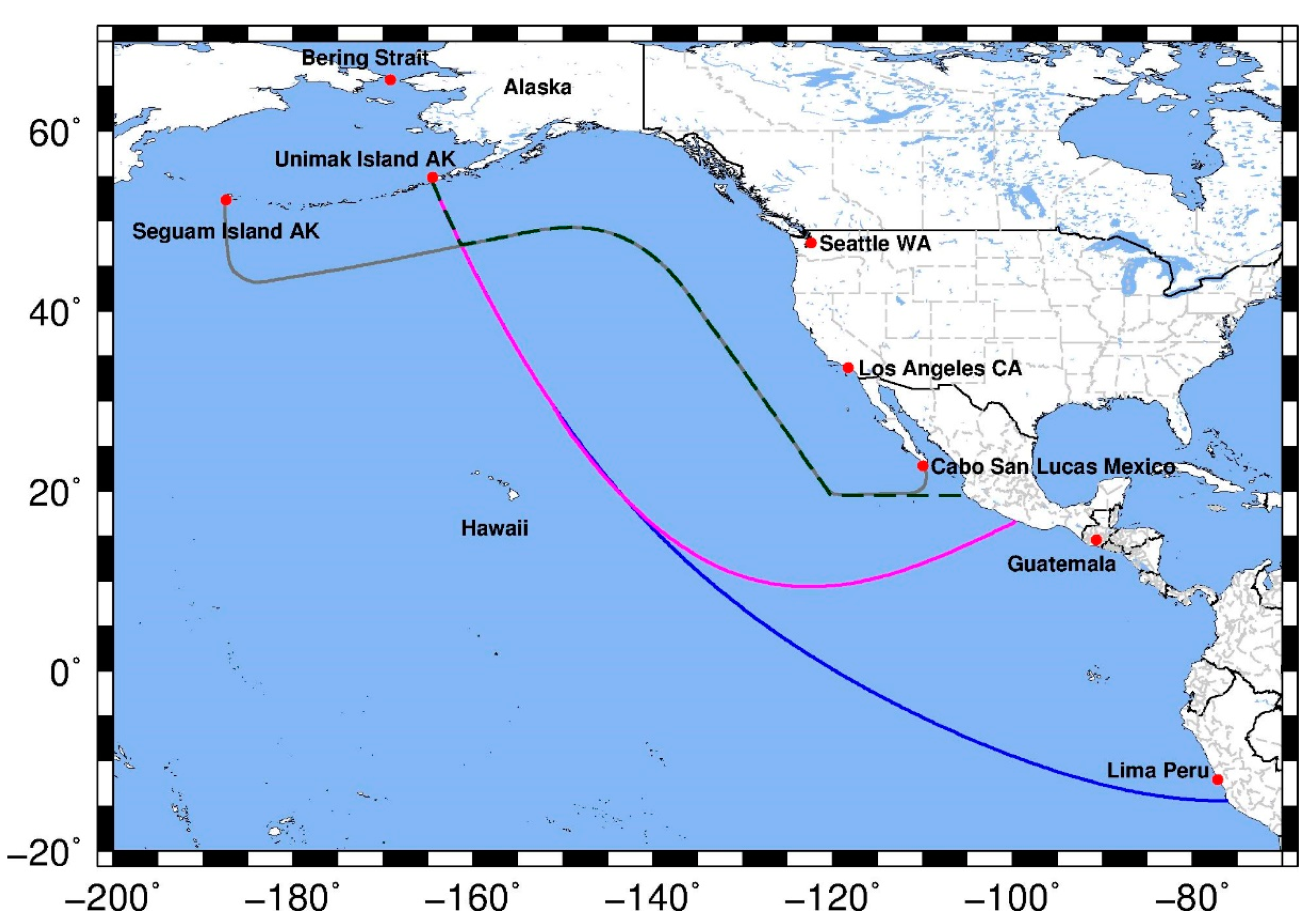
This study is concerned with the tidal response for the Pacific Ocean along the western coast of North America. This region falls within what has been called either the Northeast Pacific Region or the Eastern North Pacific (ENPAC) region, which encompasses all marine and coastal waters from the Bering Strait to the north along the west coast of North America to the Baja Peninsula and along the west coast of Mexico to the border with Guatemala [29]. Historically, three tidal databases utilizing the ADvanced CIRCulation (ADCIRC) hydrodynamic model have been developed for this region [27]; each of these databases developed the tidal profile within the domain by forcing the open ocean with global tidal data. Figure 1 presents these historical database domains, as well as the current database, (only open ocean boundaries shown) within the geographical ENPAC region. Note that, although these databases do not encompass the entire geographic region, it is convenient to use the ENPAC abbreviation.
The tidal database for the Eastern North PACific region was originally developed in 1994 (called ENPAC1994); it utilized an unstructured grid and resolution varied from about 15 km along the coast to 60 km in the open ocean. Bathymetric information was obtained from the 1988 version of the Earth Topography 5-arc-minute grid (ETOPO-5) [30]. However, the results from this tidal database did not provide good agreement with the field data, and, in some areas, did not provide any improvement over the global ocean tidal models [27].
The first update was not undertaken for nearly ten years; ENPAC02 included increased grid resolution, a reduction of the overall domain and updated bathymetric profiles. Bathymetry was defined from the available National Ocean Service (NOS) soundings database and the 1998 version of the ETOPO-2 product [31] where soundings were not available. The domain extent was reduced to avoid the cluster of tidal amphidromes off the South American coast. The final ENPAC02 model had grid resolutions ranging from about 8 km along the coast to 60 km in the deep ocean. The combination of improved bathymetry, increased coastal resolution and reduction in the domain extent improved the results with the ENPAC02 database; however, major problems persisted with the amplitude and phase of the semi-diurnal constituents [27].
In 2003, further changes were made to the domain extent, primarily moving the boundary closer to shore; the area eliminated was a portion of the deep ocean waters where the amphidromes associated with the semi-diurnal constituents resided. Additionally, the entire coastline was resolved, even further resulting in an average coastal resolution of 1 km. These modifications to the model domain led to increased accuracy in the tidal results, particularly the semi-diurnal constituents, and the database was released as ENPAC03; it provided elevation harmonics for the eight major tidal constituents and three nonlinear constituents (K1, O1, P1, Q1, M2, S2, N2, K2, M4, M6, steady) at any location within the domain [27].
The latest version presented herein, ENPAC15, has significantly enhanced coastal resolution with a minimum element size of 20 m along small channels and man-made barriers and an average element size of 65 km at the open boundary. Typical resolution along the mainland United States coastline is 200–400 m; at this time, the Alaskan coastline has not been updated and resolutions in that area range from 2 to 5 km. The ENPAC15 database provides the amplitude and phase for the 37 standard NOS tidal constituents [32] for both elevation and velocity. The model domain features of the various ENPAC tidal databases are provided in Table 1.
With each successive update, the ENPAC databases have gained accuracy in the internal tidal signals. However, the previous database (ENPAC03) still has significant errors (13% amplitude and 13° phase globally), particularly in the region near Vancouver Island where the interior passages have not been resolved (average errors of 22% amplitude and 25° phase). Furthermore, data availability and technological advancements in the past 10 years provide even greater levels of model sophistication and domain complexity. The overarching objective of this study is to reduce the global and regional errors of the ADCIRC tidal database in the ENPAC region. We realize this objective by incorporating six improvements into the latest generation tidal database: new open ocean boundary location, updated coastal resolution, updated bathymetry, boundary forcing using the latest global tidal databases, comparison of the bottom friction parameterization and inclusion of the advective terms within ADCIRC.
In the following sections, these improvements and the resulting error reductions are presented. The development of the ENPAC15 tidal constituent database and validation methods are summarized in Section 2; skill assessment for global, regional and site-specific locations are provided in Section 3 and a discussion of the results and limitations of the database are provided in Section 4. In the interest of brevity, the skill assessment only covers the eight primary constituents: M2, S2, N2, K2, O1, K1, P1 and Q1.
2. Materials and Methods
The methodology of this study closely follows that used for the development of the EC2015 tidal database for the eastern coast of the United States [26]; therefore, the entire outline and much of the text provided in Section 2.1, Section 2.2, and Section 2.3 is similar to that of our previous study (in order that this paper is complete enough to stand alone for those readers who are not familiar with that study). While the methodology is similar, it is not the same, due to peculiarities of local regions, so readers are cautioned not to skip these sections entirely. In particular, the subsections within Section 2.2 are region specific to ENPAC and are important for thorough understanding of this current study, as are the discussion of the validation data and methods in Section 2.3.
2.1. ADCIRC Computational Model
2.1.1. General Model Details
The enhancements to this database employ the ADCIRC regional hydrodynamic model. ADCIRC utilizes the full nonlinear shallow water equations, using the traditional hydrostatic pressure and Boussinesq approximations. The depth-averaged generalized wave continuity equation (GWCE) is used to solve for the free surface elevations, while the non-conservative form of the momentum equation is used for the velocity components. There have been many papers written about the development and usage of the ADCIRC computational model, but basic details for the equations of ADCIRC can be found in [33,34,35].
One of the advances within ADCIRC since the West Coast database was last updated in 2003 is the addition of Manning’s n to represent bottom friction. Users can now specify specific quadratic friction coefficients, Chezy friction coefficients or Manning’s n values throughout the domain. For the Manning’s implementation, the n values are converted to an equivalent quadratic friction coefficient within ADCIRC (for each node and at every time step) before the bottom stress is calculated [36]. Note that the computed quadratic friction coefficient can also be limited on the lower end by specifying the minimum CF value; otherwise, the values can become quite small as the depth becomes large.
2.1.2. Model Input Parameters
Unless otherwise noted in the appropriate methods and results’ subsections, all the ADCIRC model runs used the parameters in the following descriptions. To capture the long-period nonlinear tides, the ENPAC15 tidal database was developed from a 410-day simulation. The model was run from a cold state (zero elevation potential and velocity) and a ramp was applied to both the boundary forcing and the tidal potential forcing functions for the first 25 days. Then, the model was run for another 20 days before the internal ADCIRC harmonic analysis was started for the final 365 days of the simulation (a one-minute interval is used for the internal harmonic decomposition). Tidal potential forcing was applied to the interior of the domain for the eight primary constituents (O1, K1, Q1, P1, M2, N2, S2 and K2). In addition to these, the open ocean boundary was also forced with two long-period constituents (Mm and Mf). Tidal boundary forcing was extracted from the OTIS TPXO8-atlas global tidal database [37].
A time-step of 1.0 sec and the default time weighting factors (0.35, 0.30 and 0.35) were used. The lateral eddy viscosity coefficient was set equal to 5.0 m2/sec. With the exception of the various bottom-friction comparison runs, a nonlinear quadratic bottom-friction scheme with a constant value of 0.0025 was used. Specific friction settings for the Manning’s n formulation and the variable CF runs are detailed in Section 2.2.5 below. The traditional spatially variable but temporally constant GWCE weighting parameter was used (τ0 = −1). Finally, variable Coriolis forces were enabled and the nonlinear finite amplitude option was utilized with wetting and drying enabled.
2.2. Improvements for the ADCIRC Tidal Database
Since the development of the ENPAC03 tidal database, many advances have occurred in global tidal databases, available coastal data, options within ADCIRC itself and general computing capability, thus allowing for the inclusion of additional coastal inland areas. For this current ENPAC tidal database, six areas of improvement were examined:
- Assess the location of the open ocean boundary.
- Improve the coastal resolution using the National Oceanic and Atmospheric Administration (NOAA) Vertical Datum Transformation (VDatum) product grids.
- Update the deep-water bathymetry.
- Use the latest global tidal database products for forcing on the open ocean boundary.
- Compare three bottom friction schemes for improved accuracy.
- Improve the model physics by enabling the advective terms within ADCIRC.
In the following subsections, the methods used for each of these areas are detailed. Actual improvements realized in the harmonic constituent accuracy will be presented in the results section.
2.2.1. Open Ocean Boundary Placement
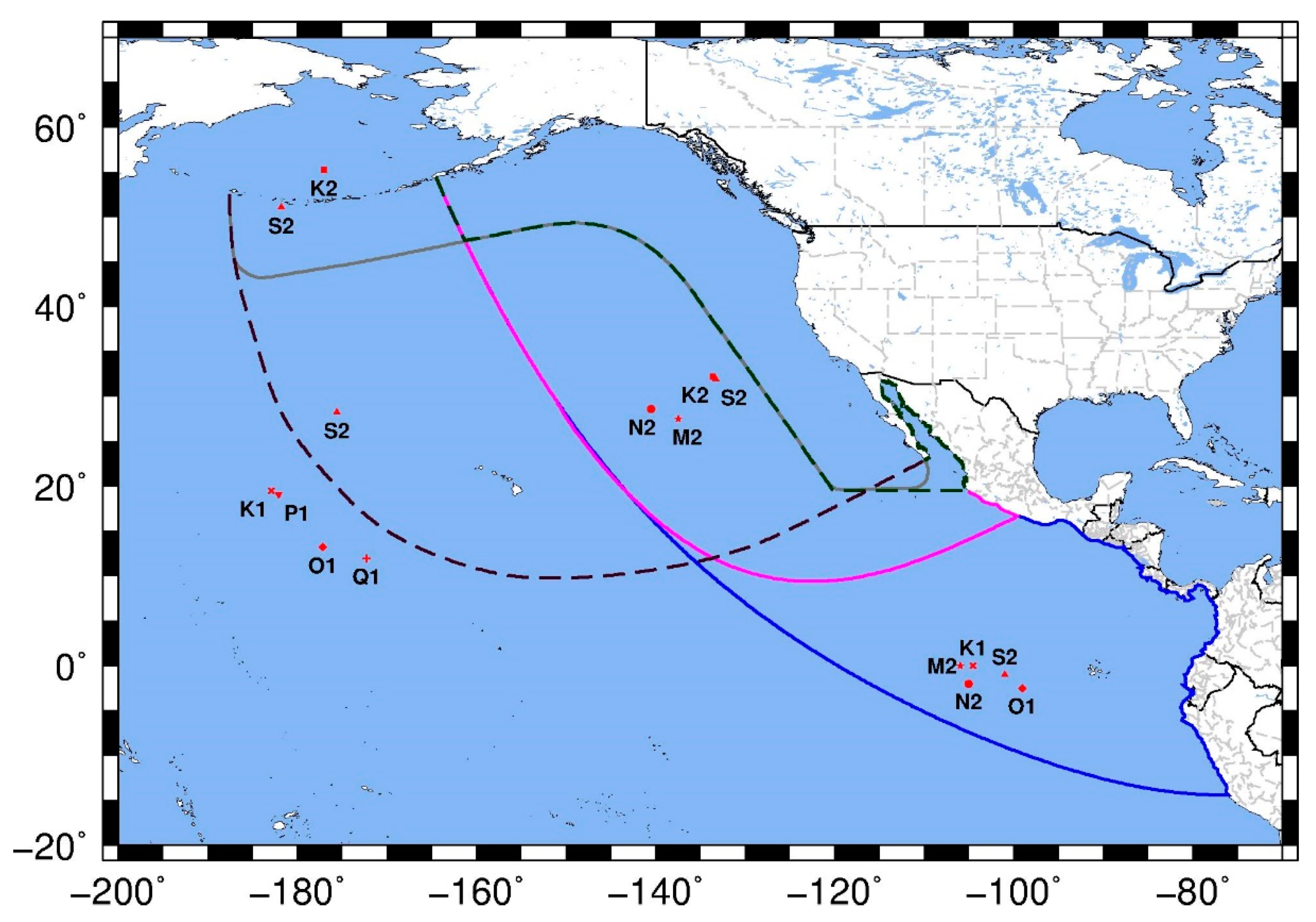
While the removal of the amphidromic points from within the model domain significantly improved the results of the ENPAC03 database relative to the original 1994 database, the original intent of the ENPAC15 model was to include the Hawaiian Islands in the model domain. The operational mesh used by the Extratropical Surge and Tide Operational Forecast System for the Pacific Ocean (ESTOFS-Pacific), which was put into operation in June of 2014, was a good candidate for such an attempt [38]. Figure 2 shows the ESTOFS-Pacific model domain, along with the location of nearby amphidromic points and the various ENPAC domains.
During the development of the ESTOFS-Pacific model, it was determined that the semi-diurnal constituents were underestimated along the coast, particularly along Alaska. In order to mitigate that this in the operational framework, a 20% increase of the semi-diurnal amplitudes along the open-ocean boundary had to be implemented [38]. While this fix was workable in the operational system (where the extended domain is necessary) and the amplitude errors at the Hawaiian Island stations were within acceptable bounds, it was determined that the over estimation at these island stations would not be acceptable in a tidal database. Furthermore, past experience with ENPAC1994 and ENPAC03 clearly indicate that the presence of the amphidromic points for the semidiurnal constituents within the domain degrades the harmonic results for the same constituents. Therefore, the coast-hugging paradigm of the earlier databases, which avoids these amphidromes, was continued for this version of the database, with the understanding that the Hawaiian Islands can be modeled with boundary conditions extracted from global tidal databases.
Further tests on the ENPAC03 model domain revealed that the presence of the shelf break across the open ocean boundary to the west prevented stable runs when ADCIRC’s advective terms were enabled for use (this was confirmed upon examination of the ENPAC03 report as well [27]). Experience gained while updating the Western North Atlantic ADCIRC tidal constituent database revealed that the advective terms played an important role in reducing errors in the shallow near-shore regions [26]. In order to avoid the S2 amphidrome off the Aleutian Islands, an attempt was made to extend the ENPAC03 domain just west of the shelf near longitude −180°. Unfortunately, this was unsuccessful and the model was still unstable at the north-west extents of the open ocean boundary when the advective terms were utilized. Therefore, it was decided to extend the north-west boundary all the way out to the ESTOFS-Pacific extents, as that domain was stable when the advective terms were implemented. Although this incorporates one amphidrome within the domain, accuracy within that region of the model domain is already compromised by the treatment of the Aleutian Island chain as a closed mainland boundary—thus neglecting the interaction with the Bering Sea. Therefore, further inaccuracy in that immediate area was tolerable, with the caveat that the tidal database should not be used to extract boundary conditions for any points west of longitude −164.5° (Unimak Island, AK) where the previous ENPAC03 model domain ended.
Furthermore, the Baja Peninsula was also trimmed from the ENPAC03 model to remove any shelf issues on the south-east extents of the open boundary. The final open ocean boundary was chosen to curve smoothly from about Cabo San Lucas, Baja California Sur, Mexico to Seguam Island, Aleutians West, Alaska and hug the coast in a similar manner to the ENPAC03 model. Figure 2 above also shows the extents of the various ENPAC tidal database domains in relation to the ESTOFS-Pacific domain, as well as the approximate locations of nearby amphidromic points. Note that the ESTOFS-Pacific mesh was trimmed to the ENPAC15 ocean boundary for initial testing of the boundary location before the coastal resolution was increased; this mesh is referred to as ESTOFS-trim.
2.2.2. Increased Coastal Resolution
With each update to the ENPAC tidal database, as data and computational resources were more readily available, more resolution has been added to the coastline. As shown above in Table 1, the latest version has about twice the number of nodes when compared to the ENPAC03 mesh.
Over the past 20 years, NOAA has undertaken an ambitious study of the United States coastline to create a tool for transformation between different vertical datums. The VDatum (Vertical Datum Transformation) tool provides a single source for accurately and easily transforming geospatial data among different tidal, orthometric and ellipsoidal vertical datums along the Unites States coast. It allows the user to combine data from different horizontal and vertical reference systems into a common system in order to create integrated digital elevation models. The interested reader is referred to the VDatum website for more general information about the VDatum tool and for regional publications [39].
In order to create accurate tidal datum fields for the coastal regions, a series of highly resolved coastal grids were developed (or are being developed) for all United States waters. At the time of this study, the two most recent VDatum models available in the ENPAC15 model domain were the Pacific Northwest and Southern California domains, which together encompass the U.S. west coast from Southern California to Washington. The domain for southeast Alaska was being developed concurrently with the ENPAC15 database and was not yet available to update the SE Alaskan coast. Individual reports [40,41] for each of the VDatum domains are available on the VDatum website.
It is important to note that the high-resolution meshes created for the VDatum project are in a Model Zero (MZ) vertical datum. The interested reader is referred to the VDatum Standard Operating Procedure manual [42], but the basic idea is that small corrections are added/subtracted from the original charted bathymetry in an iterative manner until the simulation converges to a solution. The converged solution is verified against harmonic constituent data available within the region. This was necessary because the original bathymetric sources were all in different tidal datums and no tool existed to transform them into a unified vertical datum. The resulting vertical datum of the high resolution coastline is MZ. Although, model zero is not necessarily the same as mean sea level (MSL) due to nonlinear dynamic effects, for our purposes, we have to assume that the VDatum coastline is approximately relative to MSL.
Additionally, it was desired to include the passages and channels north of Vancouver Island to better capture the hydrodynamics of the Salish Sea up through Johnstone Strait and Queen Charlotte Strait into Queen Charlotte Sound. This area has been extensively studied by the Institute of Ocean Sciences, Fisheries and Oceans Canada (IOS-FOC), who provided us with several unstructured mesh models, of which we decided to incorporate two: the Vancouver Island and Discovery Passage regions [43,44]. These meshes were used to guide our model development for that area, which could not be as detailed. Additionally, the unstructured meshes that had been modeled within a finite volume framework by IOS-FOC would not remain stable in the ADCIRC finite element framework.
As a first step, the Vancouver Island model was used as input to generate a localized truncation error analysis with complex derivatives (LTEA + CD) representation of the greater Vancouver Island region [45,46]. Then, bathymetric detail was updated where possible with the finer scale Discovery Passage model. Finally, extremely shallow regions were either removed by hand or artificially deepened. In general, the representation of that region was cut to the 3 m depth contour, unless that would eliminate important channels. If smaller channels that were important for hydraulic connectivity would be removed in this process, their minimum depth was set to 3.0 m and they were allowed to remain. As such, it is not expected that the results in the Canadian waters would be as accurate as those in the U.S. waters. However, as will be seen in the discussion of the ENPAC15 model results, the incorporation of these channels is important for accuracy in the Puget Sound region. The bathymetric profiles from the IOS-FOC models were in MSL.
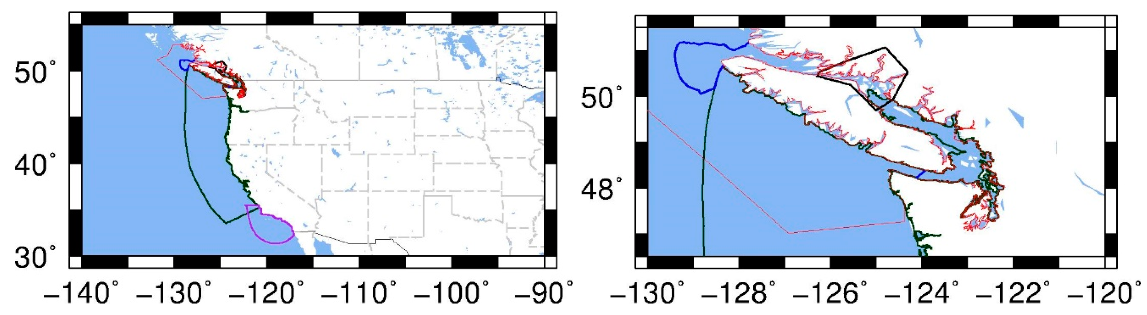
Figure 3 shows the extents of the two VDatum and IOS-FOC nearshore domains superimposed on the ENPAC15 model domain, shown to clearly illustrate the regions where coastal resolution was updated. Note that the Discovery Passage region is only a very small part of the larger Vancouver Island domain so the details are not visible at this scale. Instead, a black box is shown around the region of the Vancouver Island model where the bathymetry was replaced with the highly resolved Discovery Passage model. Also note that, in the Kitimat region, the smaller inland channels, visible in the red boundary of Figure 3 near −127.5° longitude 52.5° latitude, were not included in the final ENPAC15 domain, as we are not interested in producing tidal data in that region of the Canadian waters and we had to minimize computational requirements.
Notice that there are several areas of overlap between these regional subdomains. For the overlap in the Pacific Northwest and Southern California VDatum domains, the individual grids were carefully pieced together in such a way as to preserve the source grid with the highest coastal resolution. For the offshore regions within these overlaps, a transitional mesh was created at an appropriate distance from the shoreline that smoothly blended the triangulations of the two VDatum meshes. Finally, the bathymetry from the highest resolution source was reapplied onto the new triangulation.
A slightly different approach was taken within the Salish Sea. A transect was chosen across the Strait of Juan de Fuca at about longitude −124.0°. This location was chosen because the resolution of the Pacific Northwest VDatum mesh and the LTEA + CD representation of the Vancouver Island model from IOS-FOC was nearly the same at this location, providing a smooth transition from one model to the other. Additionally, a gentle curve just outside Queen Charlotte Strait to the southern coast of Vancouver Island was chosen as the extent at the other end of the northern Vancouver Island passages. This curve was chosen to encompass the shallow shelf off the northwestern tip of the island that was better represented within the IOS model and to ensure a smooth transition into the boundary of the Pacific NW model. Within the curved region and through the Salish Sea up to the transect across the Strait of Juan de Fuca, shown in Figure 3 by the thick blue lines, the model was taken from IOS-FOC sources. Everything outside of this region, including the triangulation for the southern coast of Vancouver Island, was taken from the Pacific Northwest VDatum mesh. However, the bathymetric representation for the southern coast of Vancouver Island was smoother in the IOS-FOC model, so the bathymetry for this immediate region was interpolated from the IOS-FOC model instead. The Puget Sound region was carefully compared to the VDatum model and it was determined that the resolution and bathymetry were essentially equivalent, with the exception of the occasional outliers in bathymetry that can sometimes occur during the model zero iterations of the VDatum process. Therefore, for ease of transition, the Puget Sound region was taken from the IOS-FOC model. Due to the ready availability of NOS data on the internet, the bathymetry sources was more than likely the same for both grids. The boundary was then smoothly transitioned into the Pacific Northwest VDatum model, in a similar manner to the process described earlier for the VDatum overlap region.
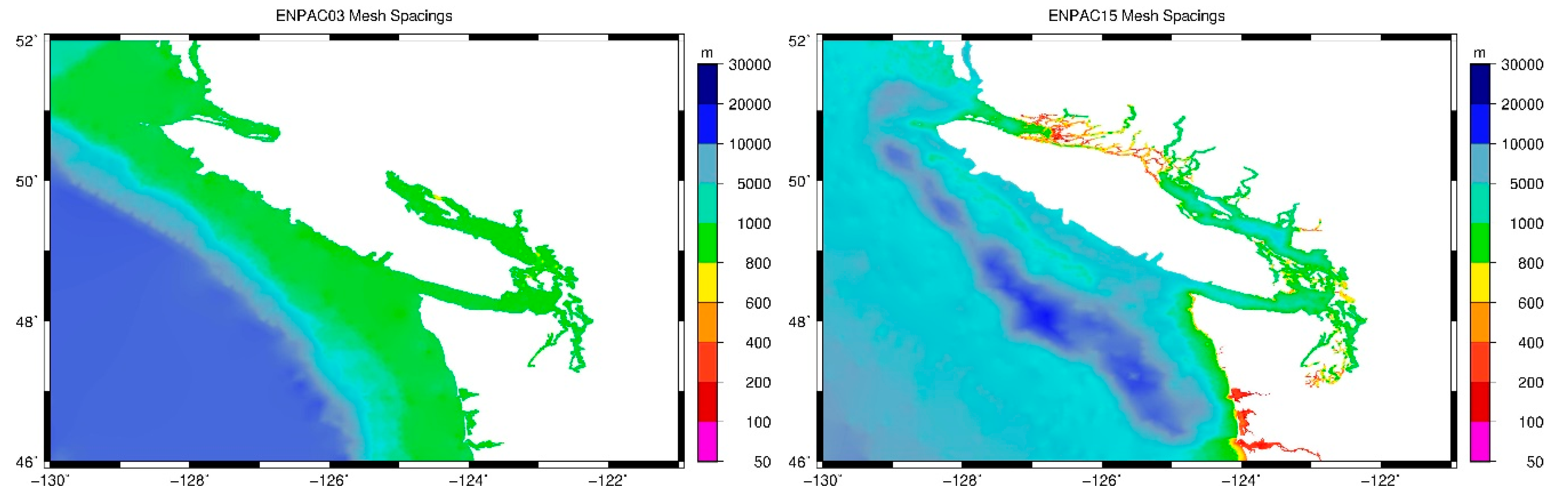
A comparison of the Vancouver Island and Washington coast region in the ENPAC15 model and the previous ENPAC03 model is shown in Figure 4. Notice in particular that the passages north of the island have been added and in general that the newest model includes more inland channels, rivers and islands, as well as a more detailed shoreline in general. Also note that the region of larger elements south of Vancouver Island is a manifestation of the LTEA + CD process, which minimizes the number of elements in deeper regions.
2.2.3. Updated Global Bathymetry
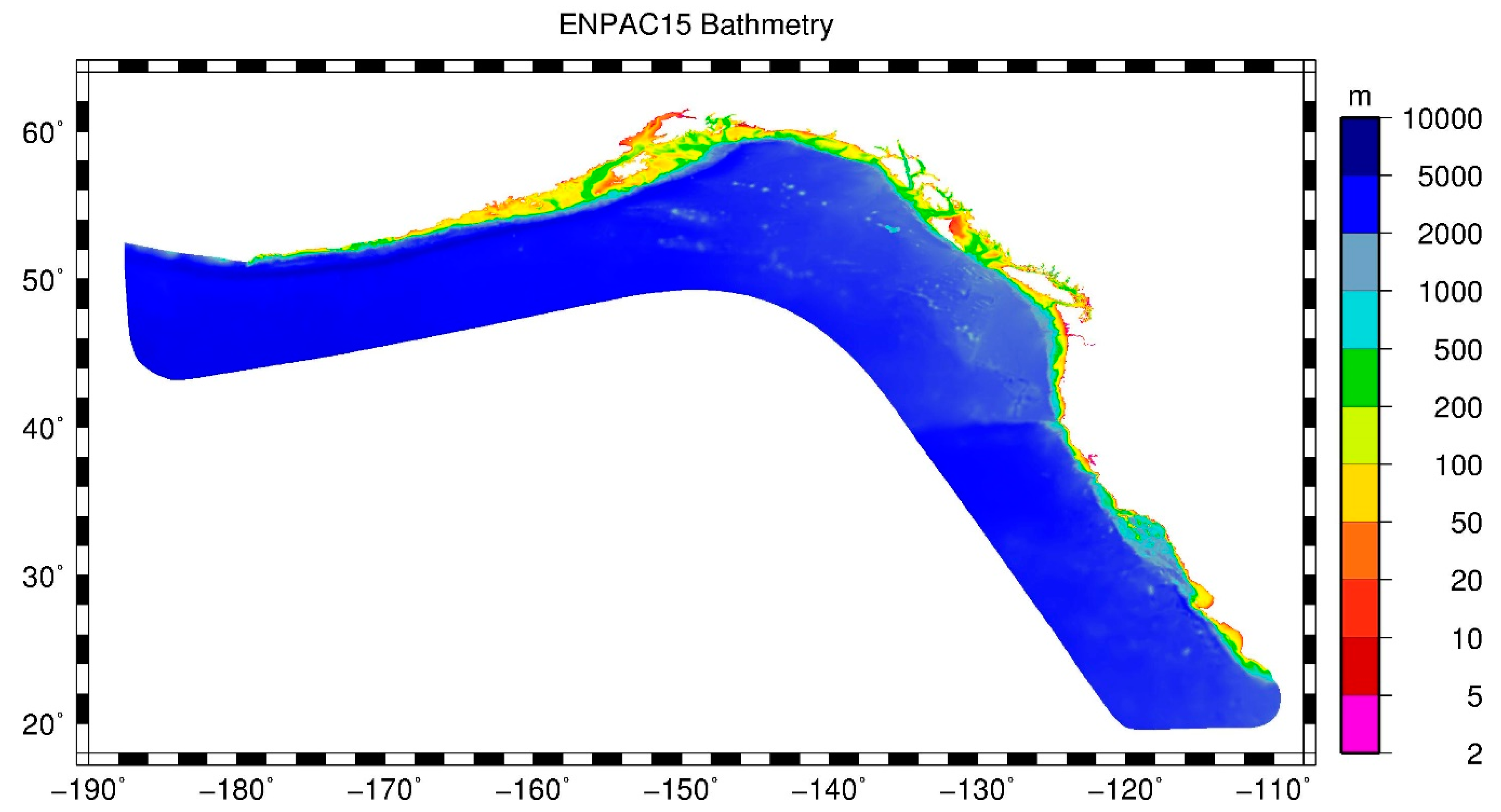
The final step of mesh development was to blend the highly resolved coastline into the global ocean described in Section 2.2.1 and update the deep-water bathymetry of the ENPAC03 model. The ESTOFS-Pacific model includes the most recent bathymetric profiles available from the National Ocean Service NOS/OCS hydrographic database maintained at the National Geophysical Data Center [47]. Additionally, the ESTOFS-Pacific model utilized the University of California-San Diego/Scripps’ global 1-minute bathy/topo dataset [48] outside of the NOS survey areas. Therefore, it was decided that the most straightforward way to update the bathymetry in regions that were not included in VDatum grids or IOS-FOC grids was to trim the ESTOFS-Pacific mesh down to the ocean boundary selected for ENPAC15. This intermediate mesh was also used for some quick comparison tests because it was not as finely resolved along the coast; it will be referred to as ESTOFS-trim. Finally, the improved coastline from VDatum and IOS-FOC sources was merged into the ESTOFS-trim domain by removing all deep water from the merged coastal regions and creating a smooth mesh out to the boundary nodes; then, the ESTOFS-trim bathymetry was interpolated back onto the regions of the mesh that did not come from the high-resolution coastal domains. The resulting ENPAC15 model bathymetry, shown in Figure 5, is referenced to MSL.
2.2.4. Updated Open Ocean Forcing
Once an updated physical model had been developed for the entire ENPAC region, it was necessary to extract tidal forcing information from available global tidal models at the open-ocean boundary. Since the last version of the West Coast ADCIRC tidal database in 2003, significant improvements have been made in the global tidal modeling community as well. Herein, we compare two global models: the Oregon State University Tidal Inversion Prediction (sometimes called the OTIS or OSU TPXO system) and the French Tidal Group Finite Element Solution database (often simply called FES). Both of these use data assimilation methods for satellite altimeter data, such as Topex/Poseidon, in the development of their global database.
The FES model utilizes a global unstructured grid to model the tidal barotropic equations in a spectral configuration and then employs data assimilation from long-term satellite altimetry data to correct the tidal signals [49]. FES products are provided on a 1/16 degree resolution for 32 tidal constituents over the global ocean. The most recent version is FES2012, which is distributed by Aviso (Ramonville St. Agne, France) [50].
The OSU TPXO system follows the same general solution techniques with a least square best fit of the Laplace tidal equations and along track averaged data from Topex/Poseidon and Jason satellite altimetry [37,51,52]. The latest TPXO8-Atlas product provides 13 tidal constituents and utilizes a global structured grid with a resolution of 1/6 degree to model the global ocean with local patches of high resolution that use local refinement of 1/30 degree around many of the global coasts.
After extracting boundary information from the FES 2012 and TPXO8-Atlas databases, a visual comparison was made of the amplitude and phase information that would be used as input into the ADCIRC model; ten constituents are used to force the model (diurnal—O1 K1 P1 Q1; semi-diurnal—M2 S2 N2 K2; and long term—Mf Mm). In general, there were very few observable differences between these two models but those that did exist were typically concentrated near the coast, which may be due to the difference in near-shore resolution between the two global models. For the semi-diurnal constituents, the amplitude differences were focused near the southern boundary at Cabo San Lucas, Mexico (refer to Figure 1 or Figure 2 for geographic locations within the ENPAC domain); while the K2 constituent also showed variation in phase along the northern boundary near Seguam Island, Alaska. Similarly, the P1 and Q1 constituents showed minor amplitude differences near both coastal boundaries and the other diurnal constituents were in good agreement for amplitude; while, for phase, the O1 constituent was consistently 11–17 degrees higher along the entire ocean boundary for the TPXO8 database but was similar for the other three diurnal constituents. Finally, for the long-term constituents, both showed minor differences in amplitude and phase all along the boundary but were in fairly good agreement considering the small amplitudes (on the order of 10−3 to 10−2 m). A more quantitative comparison was made by calculating the maximum absolute difference in amplitude and phase over all 211 open ocean boundary nodes; these results are given in Table 2. Note that there was a single outlier in the S2 constituent phase for the forcing values extracted from the FES12 database; this outlier was removed before calculating the maximum absolute differences. These observations alone were not enough information to determine if one global model was better; actual ADCIRC harmonic differences due to the boundary forcing are examined in the results section.
2.2.5. Bottom Friction Assignment
In this study, three variations of the quadratic friction formulation were compared for the ENPAC15 database: a constant CF version and two variable friction formulations. For the first variable formulation, a combination of the CF values that had been developed for each of the VDatum regions was used, while the second scheme utilized the USGS Woods Hole Coastal and Marine Science Center’s usSEABED [53] database of core samples to assign appropriate regional Manning’s n friction values.
Of the two VDatum grids that fall within the ENPAC15 model domain, only the Pacific Northwest grid had a variable quadratic bottom friction scheme. Additionally, no bottom friction information was provided for the IOS-FOC domains in Canadian waters. Therefore, the values from the one available region were simply mapped onto the corresponding region of the ENPAC15 domain. Then, the default value from that domain (CF = 0.00375) was applied as the default for the entire ENPAC15 domain as well.
The usSEABED database contains three files for each region: “EXT—numeric data extracted from lab-based investigations, PRS—numeric data parsed from word-based data and CLC—numeric data calculated from the application of models or empirical relationship files” [53]. Each of these datasets describes the data in different ways and has its own limitations; however, they can be combined to create a more extensive coverage of the seafloor characteristics. The database only covers the United States mainland coast and data was available only from about 117.00 W 32.24 N (north of the border with Mexico) to 122.57 W 48.78 N (near the SE end of the Strait of Georgia). Within this region, a multi-step process was utilized: (1) the three datasets were compared to make sure that they were in general agreement; (2) outliers from the comparison stage were removed; (3) duplicate points were preferentially taken from the EXT dataset; (4) the edited files were then combined into a single data source; (5) the combined file was then assessed and filtered one more time to remove large outliers that affected a wide region due to the sparsity of the data; and (6) finally any points that fell outside of the 1000 m bathymetry contour were removed. This final dataset was then interpolated onto the ENPAC15 model domain within the applicable region only.
The remainder of the domain was assigned shelf-wide values based on anecdotal evidence since no data was available and a depth-interpolation method similar to that used for the EC2015 database was used [26]. Namely, each larger coastal area was assigned a descriptive designation with an associated range of Manning’s n values based upon typical values from literature. After a region was classified by bed type, depth-dependent interpolation was used to assign Manning’s n values over each section of the coastal shelf. For water depths between 0 m and 5 m, the maximum value was assigned; for depths between 5 m and 200 m, values were linearly interpolated from the maximum at 5 m depth to the minimum value at 200 m depth; for depths between 200 m and 1000 m, the minimum manning value was assigned; finally, for depths greater than 1000 m the post-Ike “deep ocean” value of 0.012 was assigned. Table 3 provides the rough geographical regions that were used in this process, as well as the assigned min/max Manning’s n values.
2.2.6. Inclusion of ADCIRC Nonlinear Advective Terms
The final effort to improve the physics was to include the nonlinear advective terms in the ADCIRC modeling setup; the interested reader is referred to [54] for details about the development of these terms and equations. In practice, these terms enter in by activating two flags in the ADCIRC input control file. In all previous versions of the ENPAC tidal database, the westernmost edge of the open ocean boundary over the shelf break near Unimak Island, Alaska caused instabilities when the advective terms were activated. Therefore, it was not possible to include advection and compare how the tidal response varied due to these terms. With the new extended open ocean boundary, it is possible for the model to remain stable with these terms activated.
2.2.7. Summary of Tidal Database Improvements
Six different areas of improvement have been presented for the ENPAC15 tidal database. When possible, each model improvement was isolated to determine the accuracy improvement due solely to that component of the project. However, the updated global bathymetry and open-ocean boundary location were combined in the intermediate ESTOFS-trim modeling domain and were not studied individually (recall that the ESTOFS-trim model is a reduction of the ESTOFS-Pacific operational model trimmed down to the ENPAC15 ocean boundary). A summary of the simulations that were completed for this study, including the run designation, description, model domain, advection terms, bottom friction scheme and open ocean boundary forcing are provided in Table 4. For the boundary forcing, the textual label before the dash indicates which global tidal database was used while the number after the dash indicates how many constituents were used. In all subsequent sections, the results will be referred to by the run designation given in this table.
To confirm that we could expect a fair comparison between all results, the ENPAC03 tidal database was rerun with the same version of ADCIRC (v51.06) used in this study. Error analysis verified that the new version of ADCIRC was recreating the harmonic constituents. In subsequent sections, all reference to ENPAC03 results indicate that constituents were directly extracted from the previous version of the database at the same locations as the recent improvements. Meanwhile, the ENPAC03 model domain was also rerun with the same input parameters as the ESTOFS-trim model, including tidal forcing extracted from the global TPXO8 database at the ENPAC03 boundary. Results from this run are denoted by ENPAC03R and are used to test the effects due solely to the boundary location. Note that these were two separate reruns: one with the same input as the original ENPAC03 tidal database to verify that nothing substantial has changed in the ADCIRC model itself (results are not shown herein), and another to mimic one of the ESTOFS-trim model results for boundary comparison (ENPAC03R).
A series of simulations using the ESTOFS-trim model were conducted to test the overall effect of the various database improvements in a faster computing environment. While many such runs were conducted, only three of these tests are discussed herein for comparison of the individual effects of boundary forcing, advective terms and coastal resolution. Recall that the ESTOFS-trim model includes more coastal features than the ENPAC03 model but is not as highly resolved as ENPAC15. Finally, three bottom friction schemes were explored using the full ENPAC15 model; these are denoted by ENPAC15-CF for constant friction, ENPAC15-Vdat for VDatum friction and ENPAC15-Mann for Manning’s n friction.
2.3. Validation of the Improved ADCIRC Tidal Database
Three sources of harmonic constituent data were used to validate the new ENPAC15 tidal database; these sources are discussed in Section 2.3.1. Additionally, the various analysis techniques used to compute model errors are discussed in Section 2.3.2.
2.3.1. Validation Data
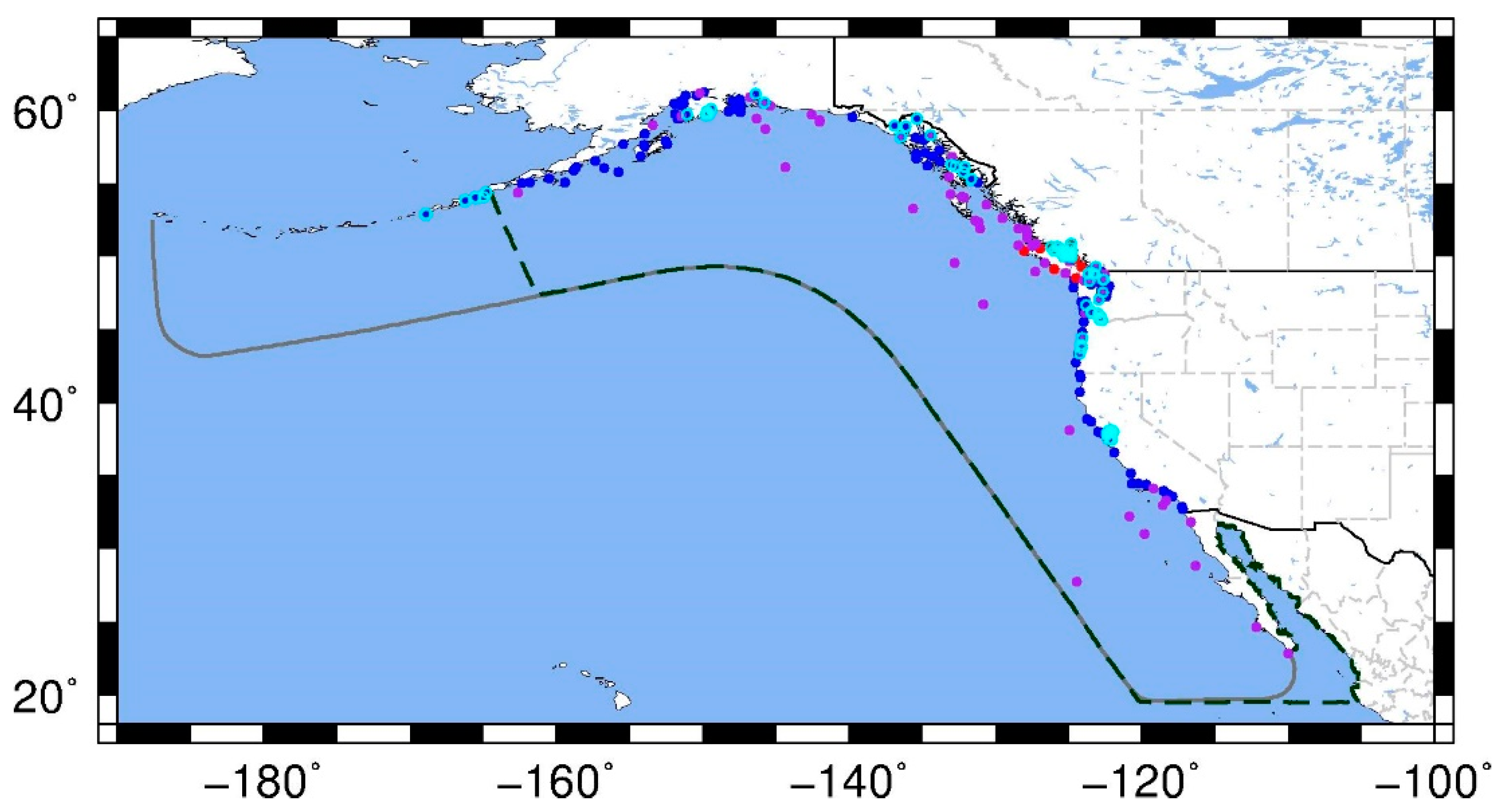
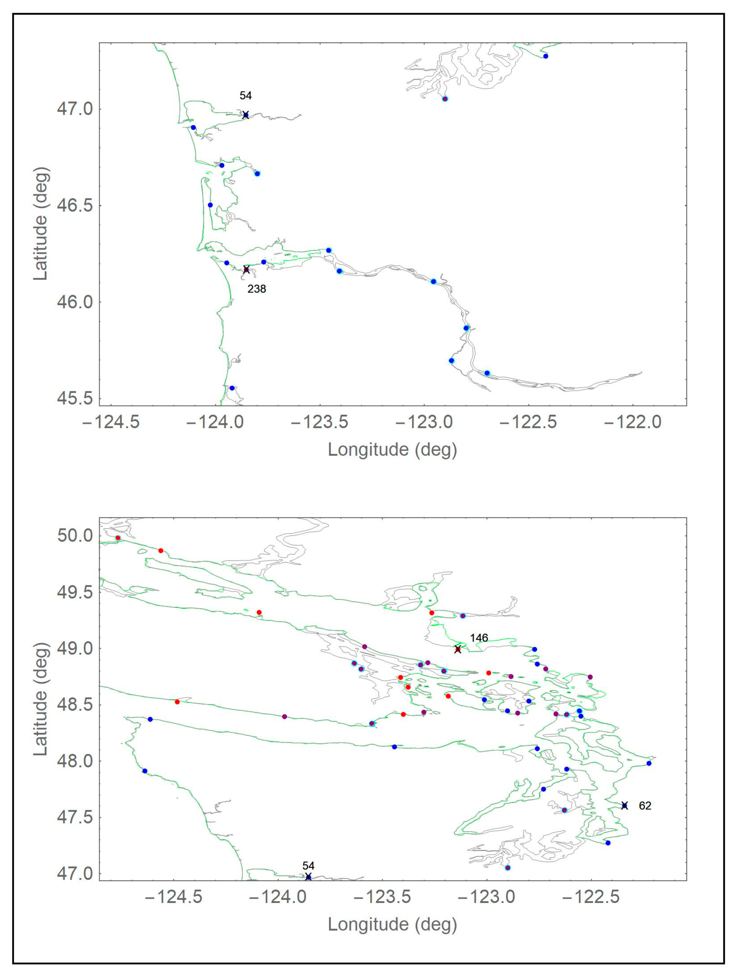
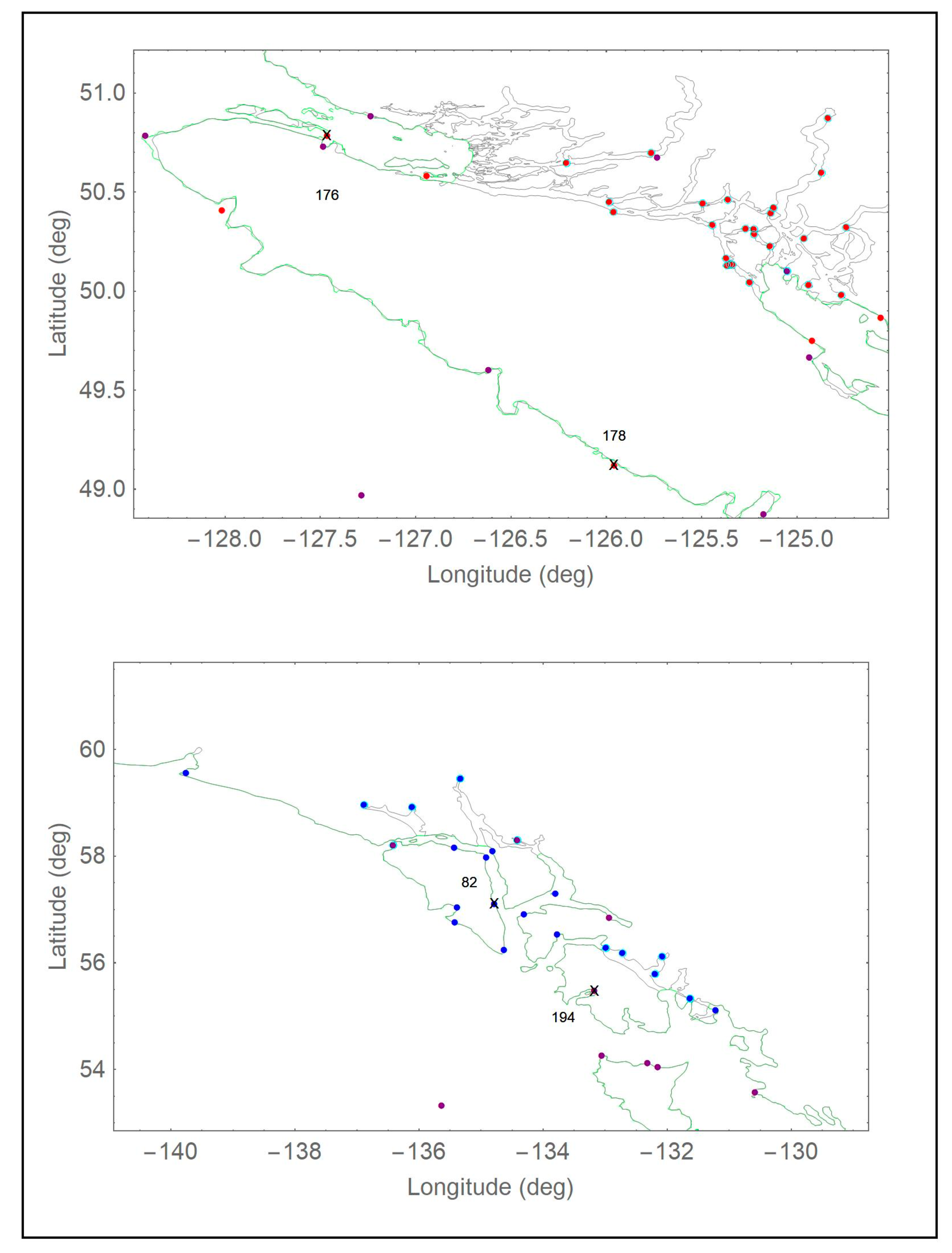
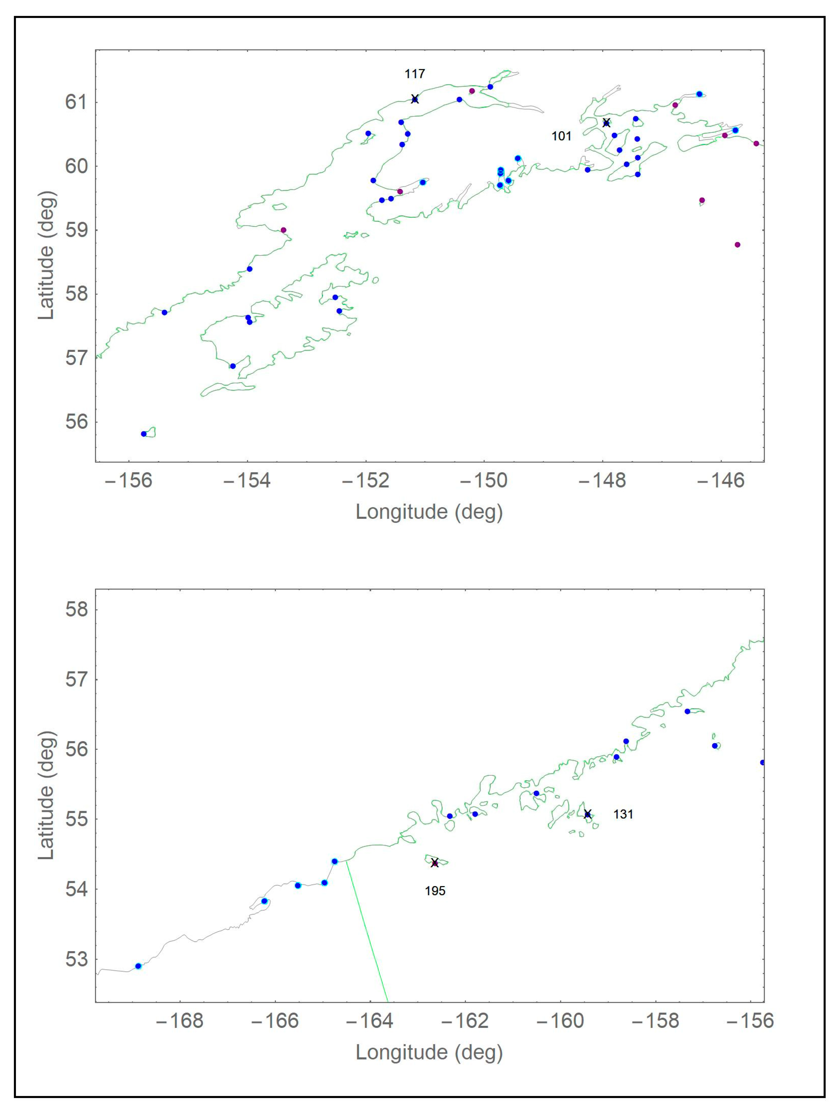
The National Oceanic and Atmospheric Administration’s Center for Operational Oceanographic Products and Services (CO-OPS) keeps a record of tidal harmonic constituent data at stations throughout the coastal United States [55]. Tidal harmonic data was available at 139 such stations in the ENPAC domain. Further data was obtained for 39 stations within Canadian waters from the Institute of Ocean Sciences, Fisheries and Oceans Canada (IOS-FOC) [56]. Finally, historical data from the International Hydrographic Organization (IHO) was used to provide wider coverage, specifically in the deeper regions [57]. There is a certain degree of uncertainty in the IHO data, as information about the source of the constituents (e.g., length of analysis and data records) is not always available; furthermore, the longitude and latitude coordinates used to locate the stations are only specified to three-decimal digits precision, which is sometimes insufficient to determine the physical location of the data collection. Of the about 4190 IHO stations available worldwide, 141 can be accurately located within the ENPAC15 domain; however, only 80 of those are unique locations not already provided in the other data sources (the 61 duplicates are used to assess the accuracy of the data itself). For skill assessment purposes, a total of 258 stations (139 from CO-OPS, 39 from IOS-FOC and 80 from IHO) were classified into three regional locations: California/Mexico, Oregon/Washington and British Columbia (Pacific Northwest) and Alaska. The global locations of the 258 available data stations are shown in Figure 6; while zoomed views with station numbers are provided in Appendix A.
Of these 258 stations, only 179 were considered “wet” in the ENPAC03 model—96 are truly within the bounds of the ENPAC03 model and the other 83 are close enough to the boundary to warrant including them (by using nearest element approximations). Stations that were far inland or within small channels that were not physically represented in the older database are not extracted from the ENPAC03 database. For Figure 6 and all the figures in Appendix A, data locations shown with a cyan circle around them are not wet in the ENPAC03 domain and are excluded from any error comparisons that specifically say that only wet stations were used. Appendix B provides a list of the station number, physical location (used for extraction from the ADCIRC databases), station name, assigned region, and the data source for all available stations.
2.3.2. Validation Methods
The same error measures as were used in the EC2015 study are used herein to determine which model best captured the tidal harmonics at the available data stations. For each station, scatter plots of measured and computed amplitude and phase were examined for the eight primary tidal constituents (M2, S2, N2, K2, O1, K1, P1 and Q1). Ideally, these plots would have a one-to-one correspondence. Scatter plots including all stations were also made for each of these eight constituents independently and a least-squares linear regression was computed. Additionally, scatter plots comparing the ENPAC03 and ENPAC15 databases for each of these eight constituents were created using 165 of the wet stations in the ENPAC03 database (fourteen of the wet British Columbia stations were neglected because they were located too close to the passages north of Vancouver Island, which were not resolved in the ENPAC03 model).
In addition to the above qualitative measures, three quantitative error measures were calculated to compare the skill of each model. For both the phase and amplitude, the mean absolute error (MAE) was computed as
where the absolute errors are summed over both the number of constituents (k) and the number of data points for a region (e). To calculate the mean errors for an individual constituent, the second sum would only be computed for k = 1 and the 8 is removed from the denominator. In all of the error plots that follow, the first eight points on the left side are for the individual constituents summed for all data stations and the regional error means are shown on the right, separated by a vertical line.
Due to some constituents having very small amplitudes, the mean relative error (MRE) was computed for amplitudes only as
where the same summation rules apply. Note that if the errors are on the same order of magnitude as the data, the relative errors will be close to 100%. Additionally, a composite error, combining the errors in phase and amplitude for each constituent into a single error metric, was computed for each station as
where Am is the modeled amplitude in meters, Ao is the observed amplitude in meters, hm is the modeled phase (degrees GMT) and ho is the observed phase (degrees GMT). As before, the mean root-mean-square error (RMSE) was computed by summing over the number of data points for any region as well as the number of constituents,
To compare the skill of the new ENPAC15 database versus the previous ENPAC03 database, harmonic constituents were extracted from the 2003 database at the stations that were within (or close enough to) the bounds of the ENPAC03 model, the wet 2003 stations. Additionally, when comparing the two database versions, only the data stations that were not located within or too close to the inside passages north of Vancouver Island were used for global statistics, even if they were designated as wet (this is due to the fact that, without the passages in the domain, the results for ENPAC03 database at these stations are not valid). Of the 179 stations that were considered wet within the ENPAC03 model, only 165 were used for global statistics; mean errors were then computed for both databases at those 165 locations. However, mean errors were also calculated at all 258 stations for the new ENPAC15 database, as it was not limited by the missing passages. Table 5 provides the total number of stations in each region that were used for statistics for each model. For reference, parenthetical numbers include only the stations that were physically within the lower resolution domains, not the nearest neighbors. Note that station details are also provided for the ESTOFS-trim model; however, in order to be consistent when comparing errors, only the 165 wet (non-passage) ENPAC03 stations are used for computing errors on this model domain.
3. Results
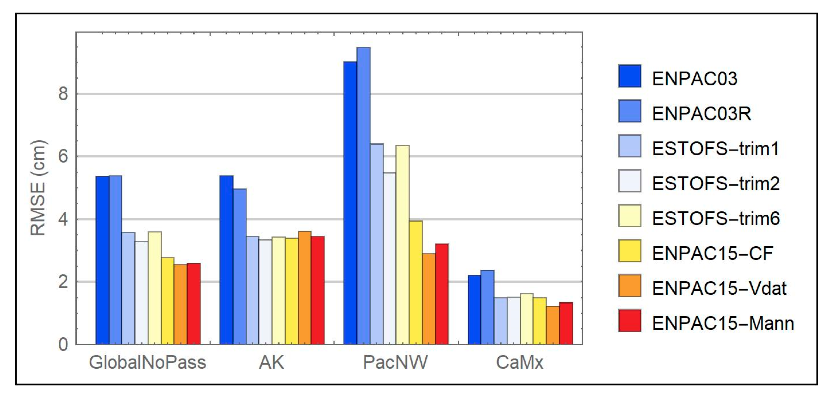
3.1. Results for the Various Improvements
In this section, some of the model improvements are examined independently to determine how each improvement affects the RMS error. Full error analysis, as described in Section 2.3.2, will be provided in Section 3.2, where the ENPAC03 model is compared to the final release ENPAC15 model. Figure 7 presents the regional mean RMS errors for all eight simulations that were previously presented in Table 4. These mean errors were computed using the 165 wet stations that are common to all model domains (recall that global statistics do not include the 14 stations that are inside the passages around Vancouver Island). Recall also that the ENPAC03R results are from a substantially different simulation than the original extraction from the ENPAC03 database. Differences include: (1) length of simulation (410-day versus 60-day); (2) nodal factors (specific factors for analysis annum 2005 versus default nodal factors); and (3) application of boundary conditions (extracted from the newer TPXO8-Atlas database for 10 constituents versus only the eight primary constituents from the TPXO6 database), such that we would not expect the resulting composite errors to be the same.
While not shown herein, it is of note that the stations located in deeper water and along the Mexican coast do not realize any significant improvements for any of the various models since the modeling domain itself is largely unchanged in this area and the most significant change is related only to the global tidal boundary forcing. Four regions are used for regional error summation: Global (without the passages), Alaska, Pacific Northwest (includes British Columbia, Washington and Oregon) and California/Mexico.
3.1.1. Comparison of Boundary Placement
As described in Section 2.2.1, the open ocean boundary has been moved further west of the shelf near the Aleutian island chain and continues to hug the coastline to avoid amphidromic points. In order to test how much of an affect the new boundary placement has on the extracted harmonic constituents, the old ENPAC03 model was run with an identical input file as was used for the ESTOFS-trim model: all input parameters are as described in Section 2.1.2.
Concentrating only on the ENPAC03R and ESTOFS-trim1 bars in Figure 7, we note that significant gains in accuracy are realized for all regions, with percent reductions ranging from 30% in Alaska to 37% in California. Unfortunately, it is difficult to determine if this is related solely to the new open boundary location or the change in resolution along the boundary itself for the ESTOFS-trim model domain. Additionally, the deep-water bathymetry was also updated in the ESTOFS-trim model, making it difficult to separate the individual effects of boundary placement, boundary coarseness and deep water bathymetry.
3.1.2. Comparison of Open Ocean Boundary Forcing
As described in Section 2.2.4, two different global tidal databases have been examined as input to the ENPAC15 model: FES12 and TPXO8-Atlas. Looking at the ESTOFS-trim1 and ESTOFS-trim6 bars in Figure 7, we note that the composite errors are similar for all regions; however, the errors from the FES12 boundary conditions are slightly higher, more noticeably in the southern region. These differences are not significant, however, and given the historical application of TPXO products for boundary forcing in the ADCIRC tidal databases and its slightly better performance in this application, it was decided to use the TPXO8-Atlas global products for this latest database update. Meanwhile, examining the ENPAC03 and EPAC03R bars, the inclusion of the two long-term forcing terms (Mm and Mf) and the updated global forcing from TPXO6 to TPXO8 does not appear to significantly affect the results; there are minor changes in the regional mean RMS errors but not globally.
3.1.3. Comparison of Advection
As described in Section 2.2.6, it was desired to include the advective terms within ADCIRC for the latest update. When examining the ESTOFS-trim1 and ESTOFS-trim2 bars, we note that while there is no noticeable difference in the California and Alaska stations, there is a significant improvement (mean RMS error reduction of 0.9 cm or 14%) in the Pacific Northwest stations when the advective terms are utilized, which also improves the global performance. Examination of individual stations in this region indicates typical mean RMS error reductions of 1.5 to 2.0 cm in the inside passages north of Vancouver Island and a maximum reduction of 3.43 cm. This is to be expected since the region north of Vancouver Island has been documented to dissipate a great deal of turbulent and internal tidal energy [43,58], which are not explicitly accounted for in the ADCIRC model. The utilization of the advective terms would allow the model to account for some of this nonlinear dissipation. However, when we turned these terms on with the fully resolved ENPAC15 model domain, instabilities developed in the shallow and narrow passageways north of Vancouver Island. Efforts are ongoing to stabilize this region (through further grid and bathymetry refinement) and allow for incorporation of the advective terms in an updated release, but for now the ENPAC15 tidal database does not include these terms.
3.1.4. Comparison of Increased Coastal Resolution
As described in Section 2.2.3, several refinements were made to the coastal geometry and bathymetry along the North American west coast. Since the operational ESTOFS-Pacific mesh (from which the ESTOFS-trim mesh was cut away) has an even coarser resolution along the coastline than the ENPAC03 model domain, we can compare the ESTOFS-trim1 and ENPAC15-CF bars in Figure 7 to get an idea of what affect this additional resolution has. Recall that we would not expect any improvement in the Alaska region because the coastal resolution was not updated in that area. Similarly, no improvement is noticed in the mean RMS errors in the California region. However, more significant improvements (38%) are realized in the Pacific Northwest stations, which reduces the global error by 22%. Much of this improvement is likely due to the inclusion of the passages north of Vancouver Island, which were previously absent from all of the ADCIRC tidal databases for the ENPAC region.
3.1.5. Comparison of Bottom Friction Schemes
In this study, three different bottom friction schemes are compared: constant CF = 0.0025, VDatum quadratic friction coefficients and Manning’s n formulation with n values estimated using the USGS usSEABEDS data. Looking at the mean RMS errors for all of the ENPAC15 bars in Figure 7, we note that both of the variable friction options (VDatum and Manning’s n) provide lower errors than the constant CF version. Furthermore, there is a slight improvement of the VDatum versus Manning’s n friction schemes. When we recall that the VDatum scheme is essentially constant everywhere except the Columbia River, then it would appear that the slightly higher default value (CF = 0.00375) is responsible for this error reduction rather than the variability of the friction itself. Additionally, we note that the friction schemes tested in this study do not appear to affect the Alaska region much at all, which might be expected since the coastal bathymetry and resolution has not been updated and most of the water is deep enough to make the friction irrelevant.
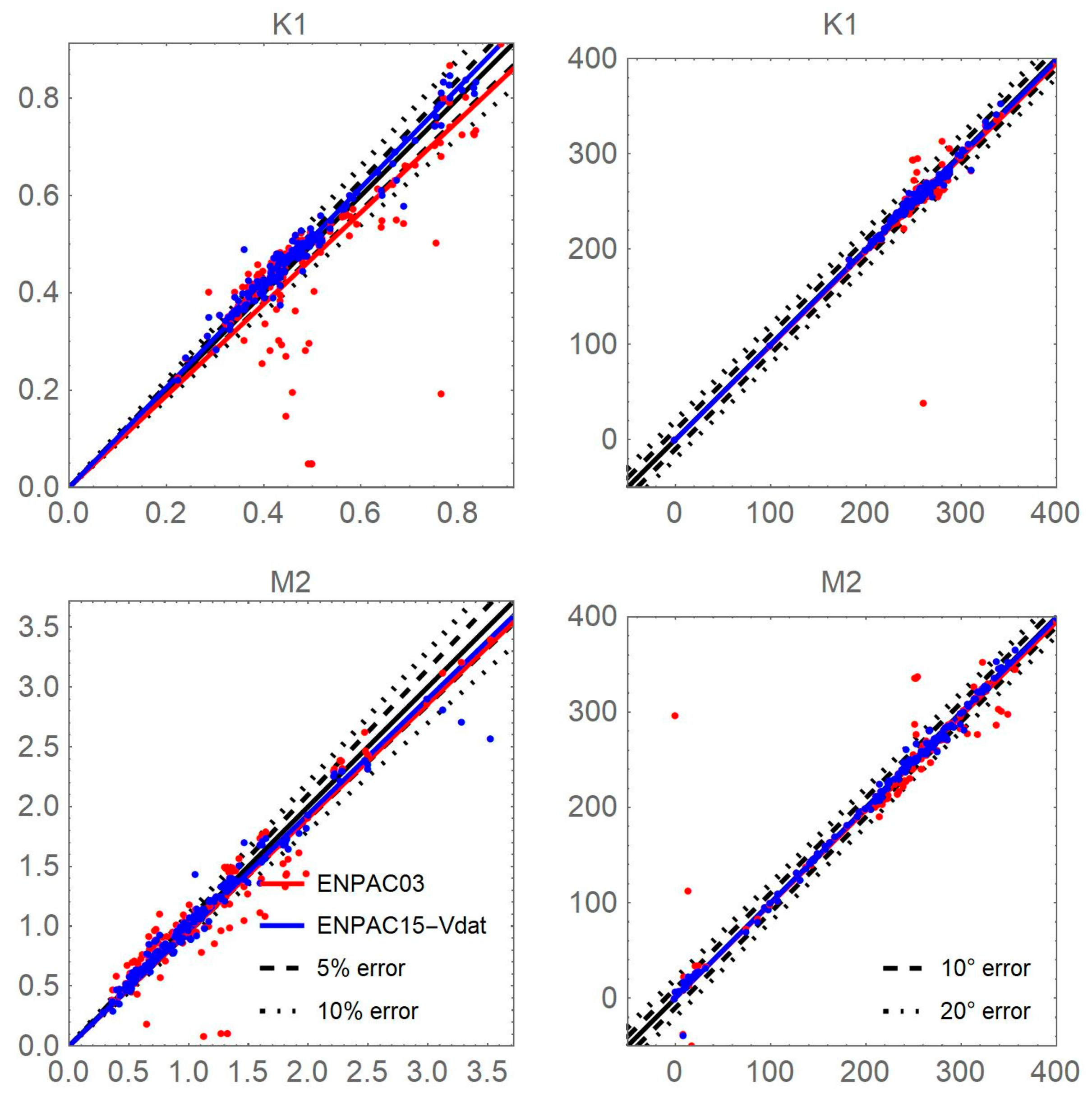
3.2. Comparison of ENPAC15 and ENPAC03
For this latest ENPAC15 tidal database release, the VDatum friction formulation was used; all other model input parameters are as described in Section 2.1.2. For results and discussion, when we refer to ENPAC03, we have extracted tidal harmonics directly from the previously released database. Scatter plots of computed versus measured amplitudes and phases (and their linear best-fit) for the ENPAC03 and ENPAC15 databases are shown in Figure 8 for the dominant diurnal and semi-diurnal tidal signals: K1 and M2. Additionally, Table 6 provides the best fit statistics for all eight primary constituents at the 165 validation stations that are common to both databases (neglecting the inside passage stations). For a perfect fit of the validation data, both the slope and R2 values would have a value of unity. Notice that the slope is improved for nearly all of the eight constituents, with the exception being O1 amplitude, Q1 amplitude and phase, and K2 amplitude; meanwhile, the R2 value is closer to unity for all amplitudes and phases, indicating a tighter distribution.
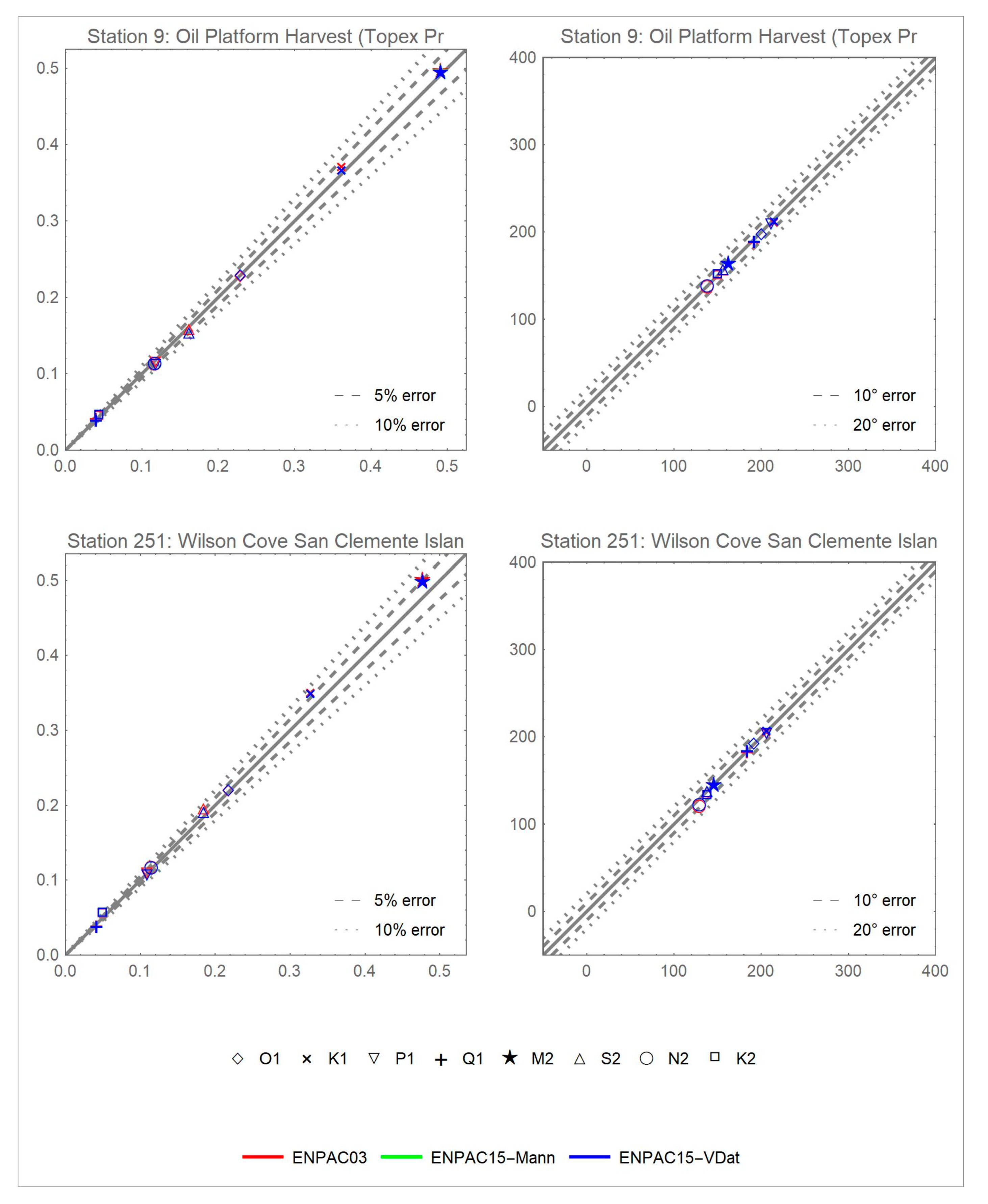
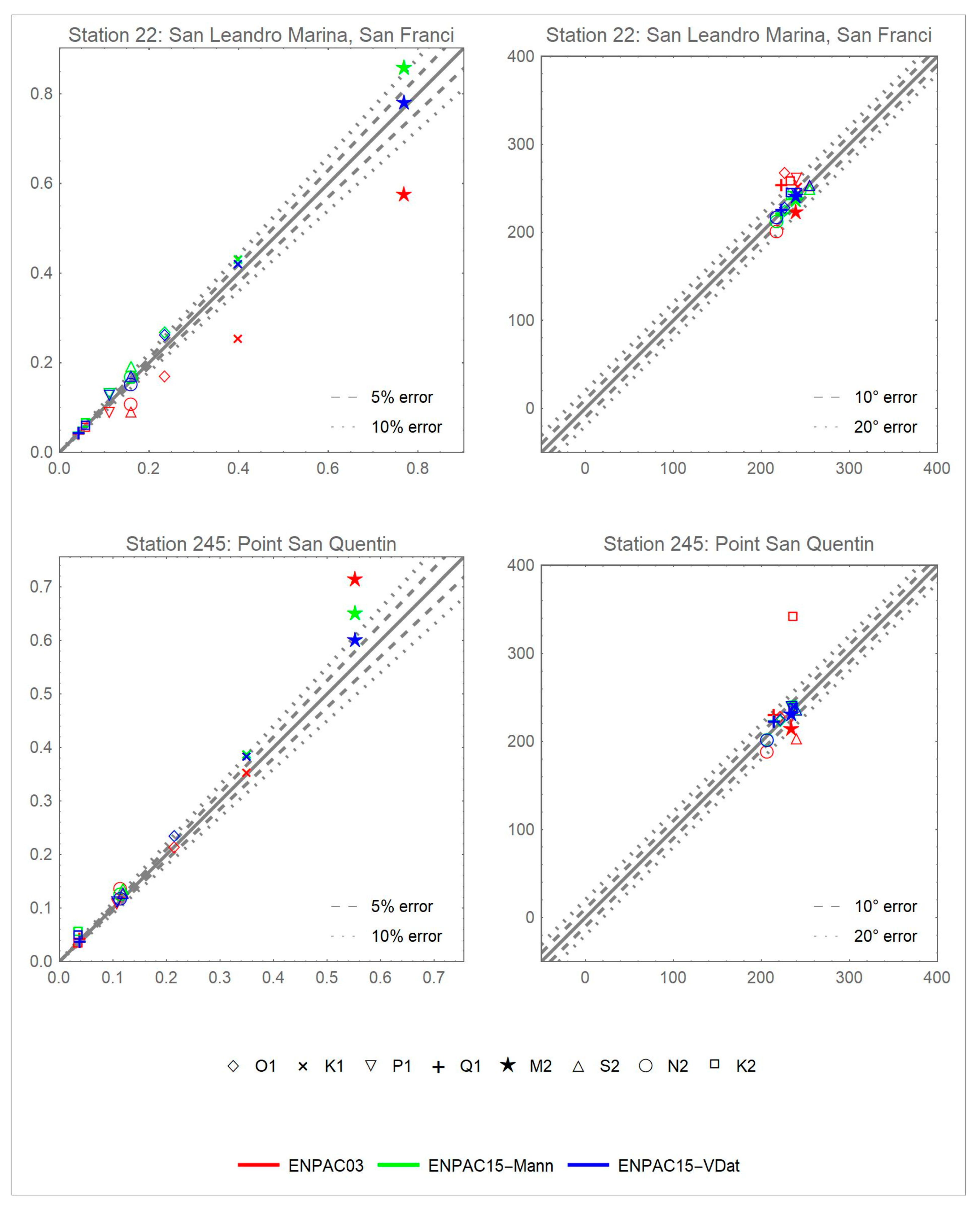
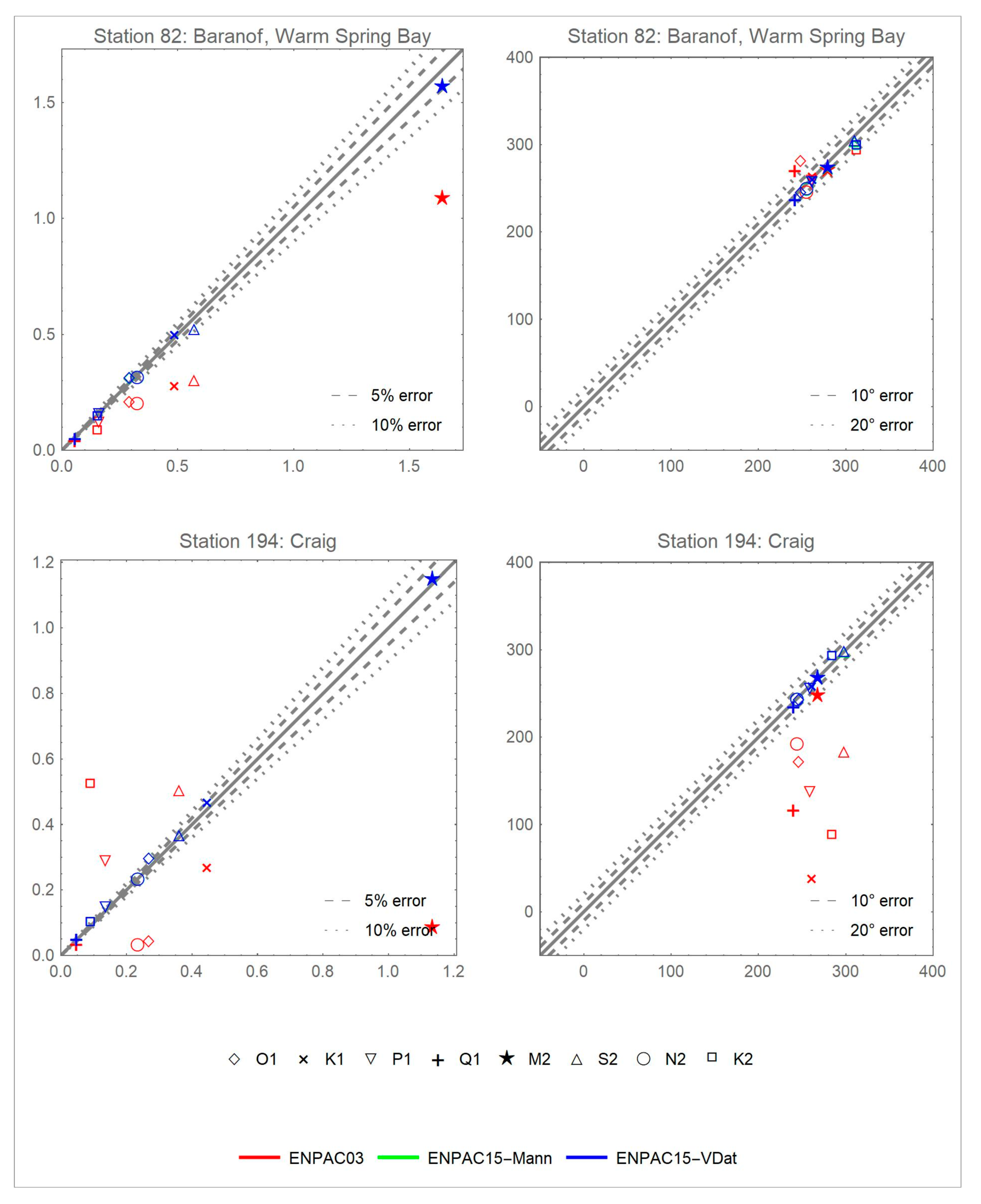
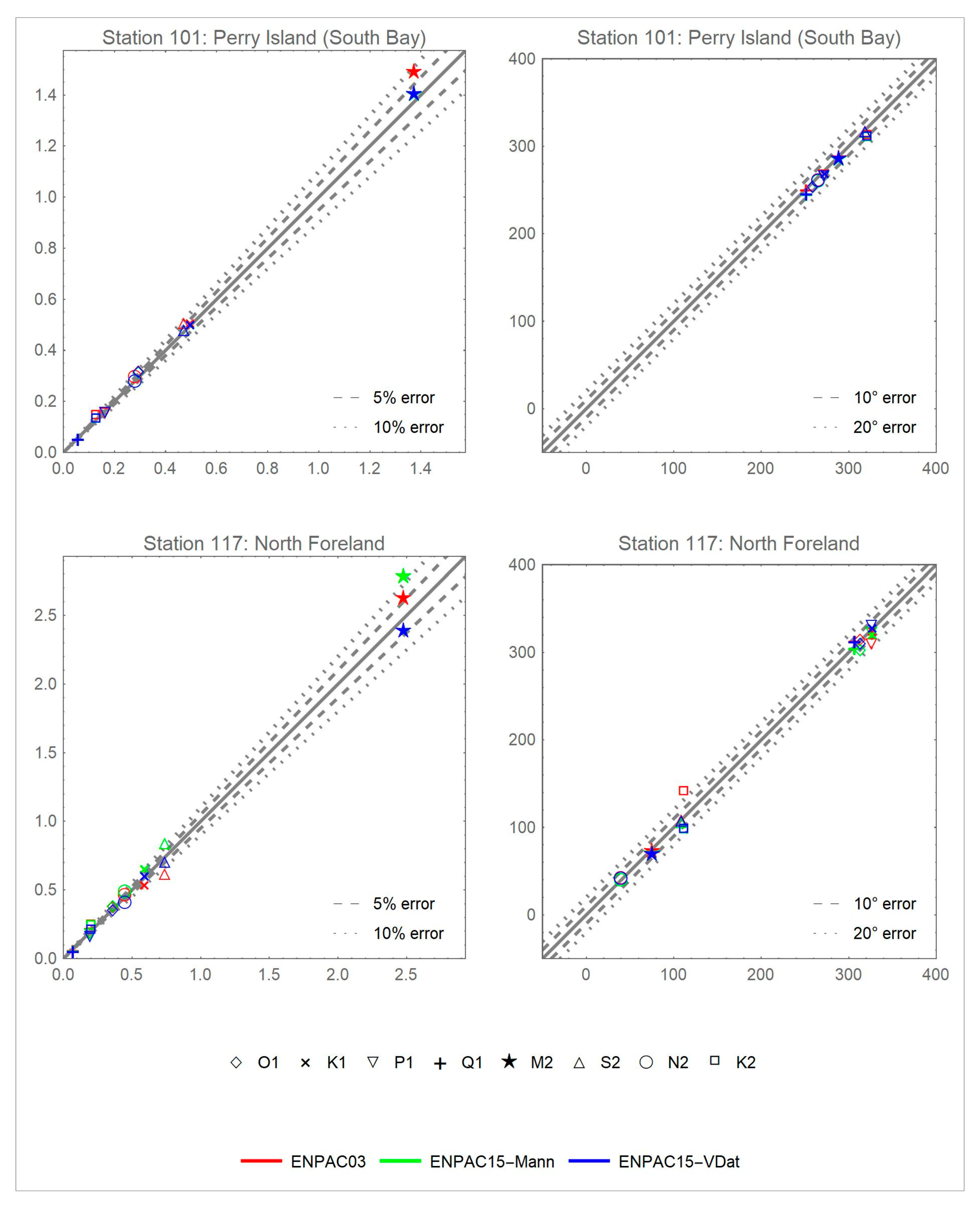
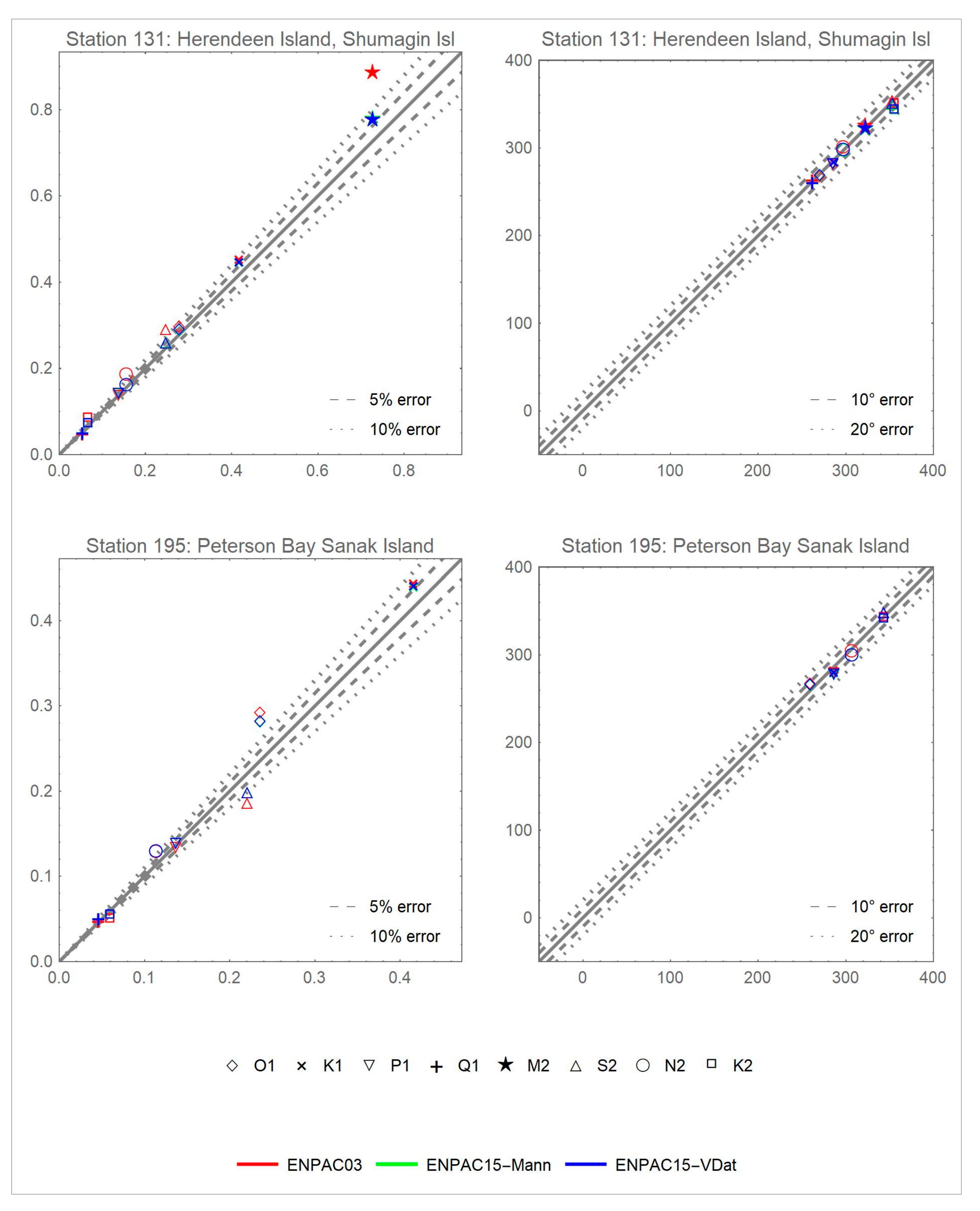
Similarly, if we look at scatter plots of individual stations, we can compare how each of the databases performs for that point. Since there are 258 validation stations, only a few representative stations are provided herein. Figure A6, Figure A7, Figure A8, Figure A9, Figure A10, Figure A11, Figure A12, Figure A13 and Figure A14 in Appendix C provide plots for the eighteen stations that were shown by a black X in Figure A1, Figure A2, Figure A3, Figure A4 and Figure A5 in Appendix A; plots are grouped together by sub region: Southern California, San Francisco Bay, Northern California, Washington/Oregon, Puget Sound, British Columbia, Southeast Alaska and Southern Alaska. In order to illustrate the station differences due to the friction formulation, results for both the VDatum and Manning’s n friction formulations are shown in these plots, along with the extracted ENPAC03 results. Other than the bottom friction itself, all other ADCIRC parameters are the same for the two newer data sets.
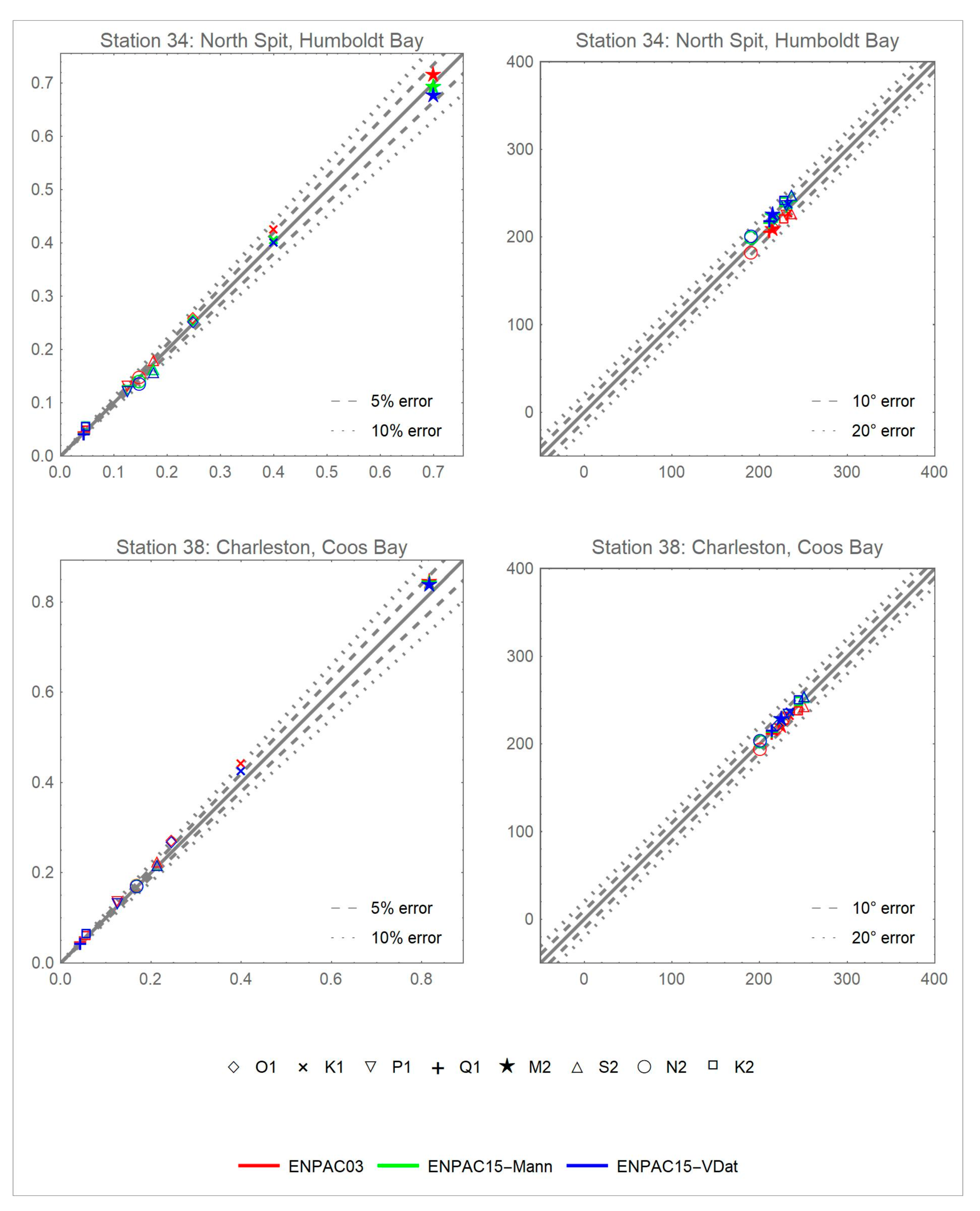
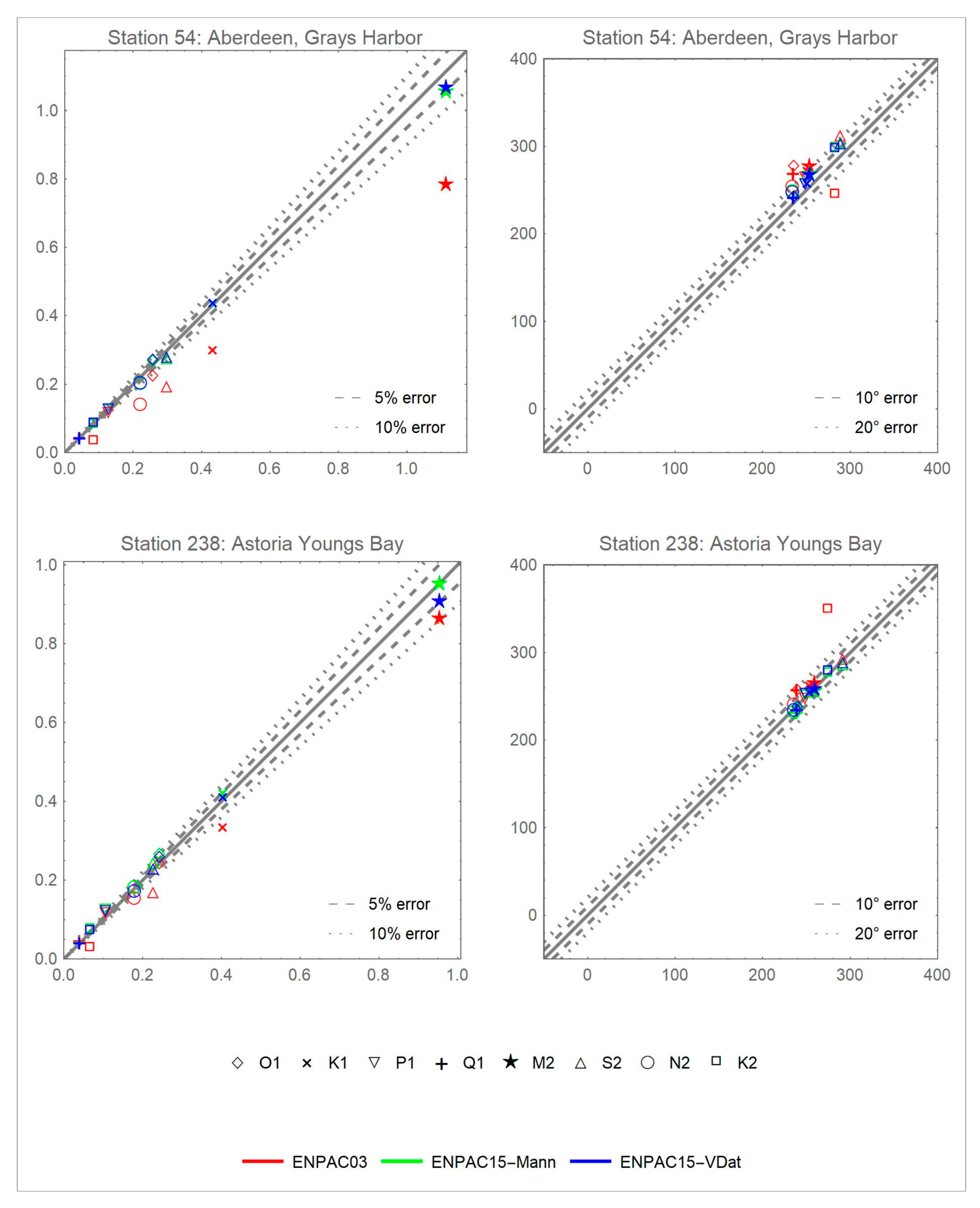
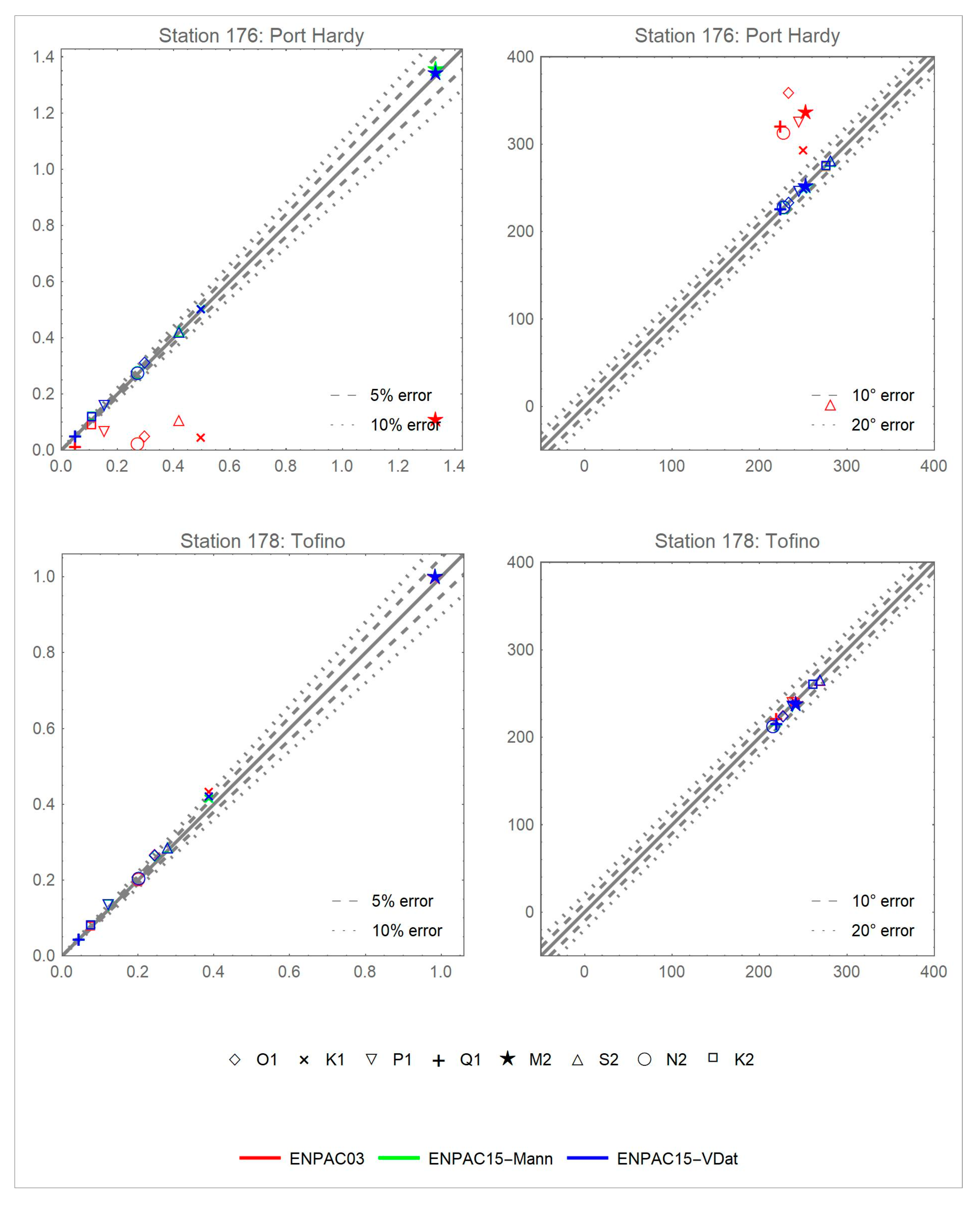
We note that very little improvement is seen in the Southern or Northern California stations (Figure A6 and Figure A7), which is expected since the coastline and bathymetry did not change drastically. However, the San Francisco Bay region is more resolved in the newer database, resulting in better amplitude and phase correspondence; note also that the friction formulation makes a significant difference in this shallower water body. Similarly, along the Washington and Oregon coasts, there is marked improvement in the new database due to the inclusion of more coastal features and upper bay water bodies. In the Puget Sound region (Figure A10), we note that the friction formulation plays a more significant role at these shallower stations; and that the phase has been improved but there is still room for improvement in the dominant amplitudes. Notice that the inclusion of the passages north of Vancouver Island has significantly improved the amplitude and phase responses at the stations on either end of the passage (stations 146 and 176), despite them being far removed from the interior passages. Results are not shown within the passages themselves, since the region was not resolved in the ENPAC03 database and no comparison can be made; however, the new database has fairly good agreement throughout this region, although the dominant constituents are overestimated. Additionally, no real improvement is noticed on the southern extents of Vancouver Island since no additional coastal refinement was added. Despite the fact that very little coastal refinement was added in the Southeast Alaska region, there are significant error reductions at these stations (Figure A12). Meanwhile, the Southern Alaska coast, which had few improvements in coastal resolution but several bathymetry corrections in this latest database, has minor amplitude improvement. Note that the results along the Alaskan coast are largely independent of the friction scheme, except for the shallower areas (station 117 in Figure A13).
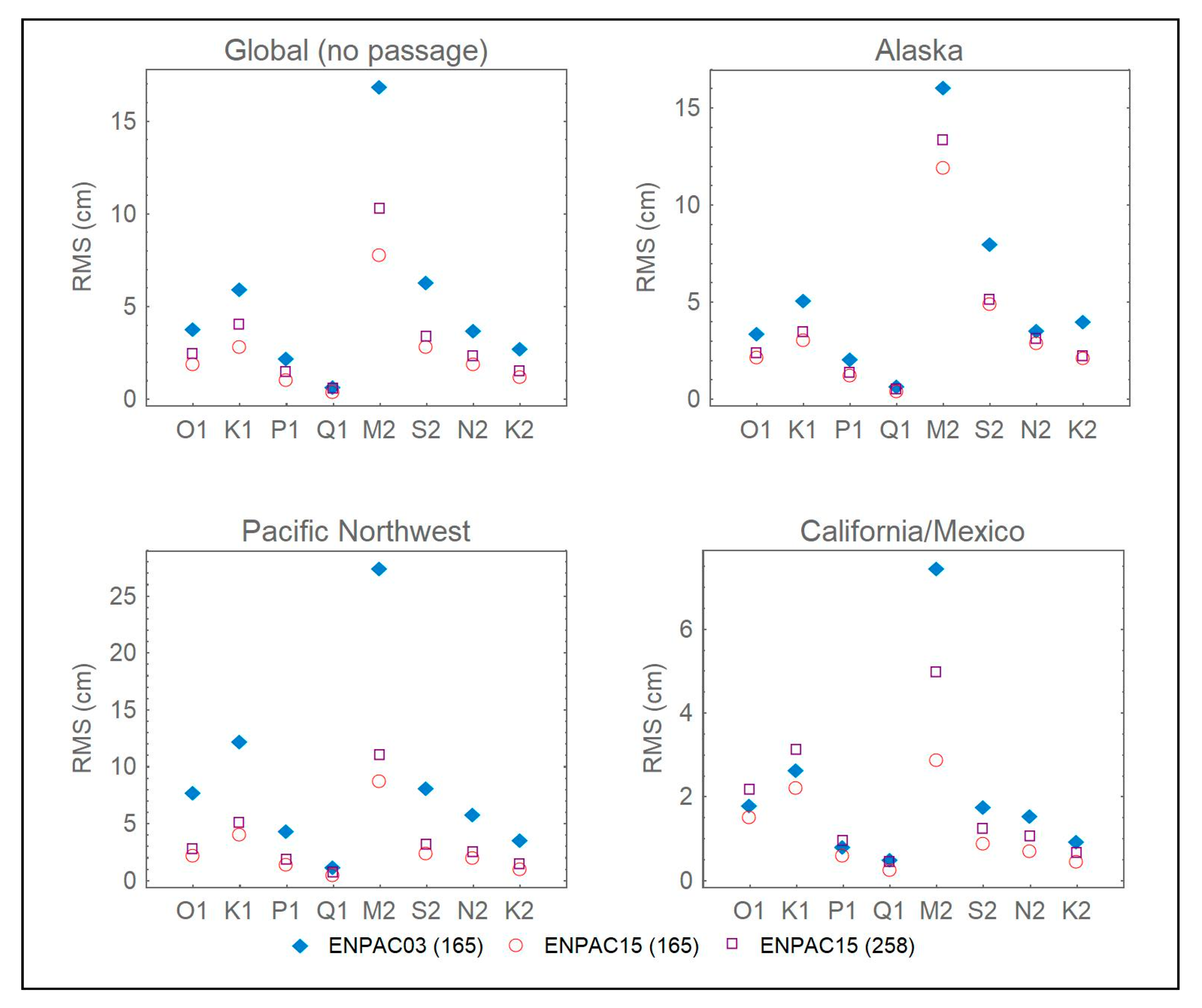
A comparison of constituent RMS errors by region are shown in Figure 9, while mean absolute phase errors and mean relative amplitude errors are provided in Table 7. Looking primarily at the 165 validation stations that are common to both databases (blue diamonds for ENPAC03 and red circles for ENPAC15), we can draw several general conclusions.
- Globally, the greatest improvement in the RMS error is realized for the M2 constituent (9 cm reduction) and the average reduction is 2.8 cm. Reductions in absolute phase errors range from 4° for the K1 constituent to 13° for the S2 constituent, with an average reduction of 8° over all of the constituents. Meanwhile, reductions in mean relative amplitude errors range from 3% for the O1 constituent to 17% for the K2 constituent, with an average reduction of 7%. For all error measures, the largest reductions were realized for the semi-diurnal constituents.
- For the Alaskan region, the reductions in RMS errors range from 0.2 cm for the Q1 constituent to 3.7 cm for M2, with an average reduction of 1.6 cm. Reduction in absolute phase errors ranged from 1.2° for the M2 constituent to 6.7° for the K2 constituent, with an average of 3.5° for all constituents, while the relative amplitude error reductions ranged from about 2% for Q1 to 20% for K2, with an average of 6%. In general, the largest amplitude reductions were realized for the semi-diurnal constituents, but the phase errors improved most for the diurnal constituents.
- The greatest improvement was realized in the Pacific Northwest region. Mean RMS error reductions ranged from 0.6 cm for Q1 to 18.7 cm for M2, with an average improvement of 6 cm. Meanwhile, the range of mean absolute phase error improvements varies from 8° for K1 to 37° for K2, with an average improvement of 21°; and the relative amplitude improvements range from 7% for P1 to 29% for K2, with an average of 13% overall improvement. The semi-diurnal constituents realize the greatest overall improvement in amplitude and phase.
- In the California and Mexico region, moderate improvements are realized; the mean RMS errors improve by 0.2 cm for Q1 to 4.6 cm for M2, with an average of 1 cm. Similarly, improvements in the mean absolute phase errors range from 0° for K1 to 6.2° for K2, with an average improvement of 2.6°, while improvements in the relative amplitude errors range from 0.6% for O1 to about 8% for Q1, with an average improvement of 4% overall. Again, the semi-diurnal constituents realize the greatest overall improvement in amplitude and phase.
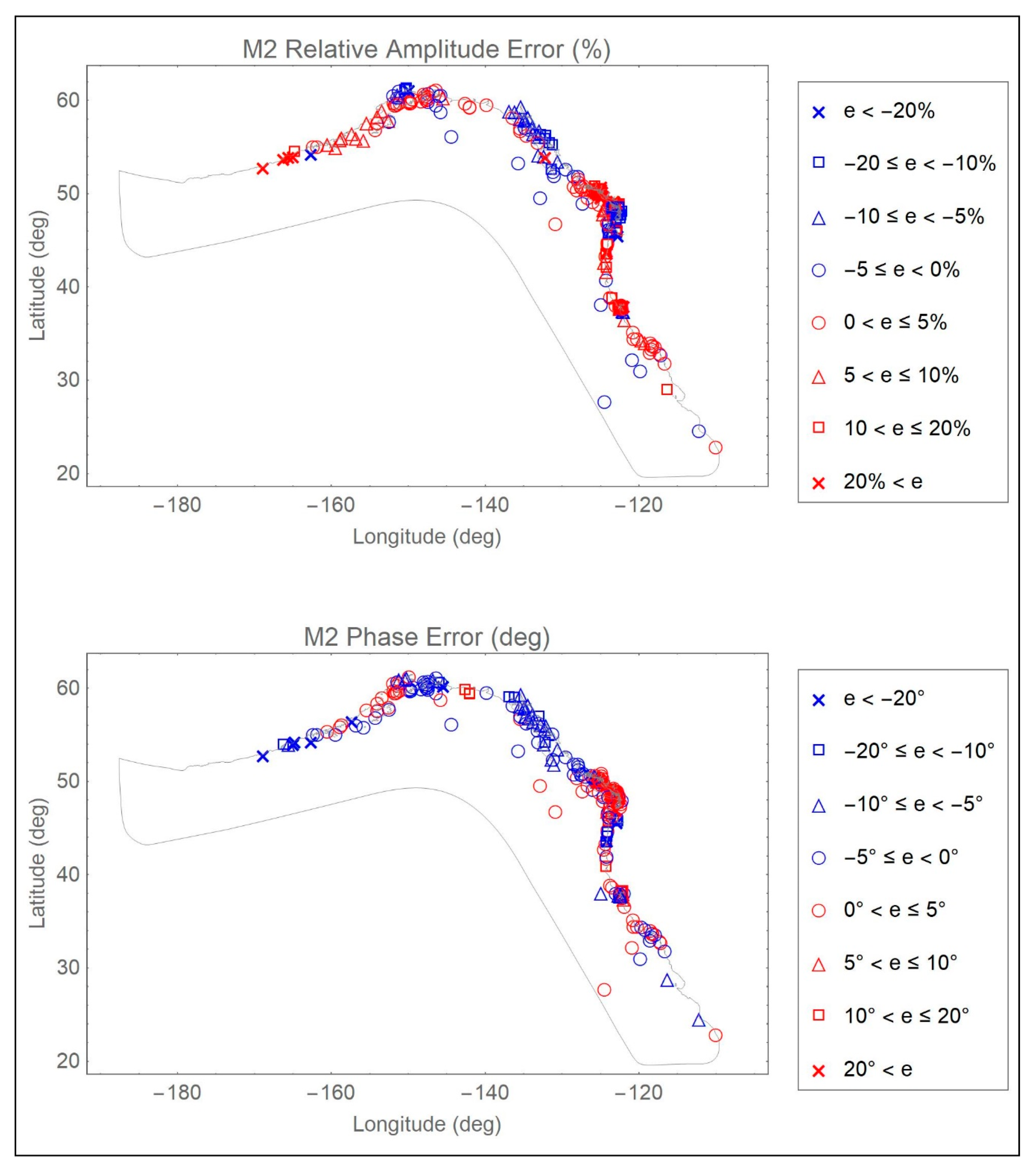
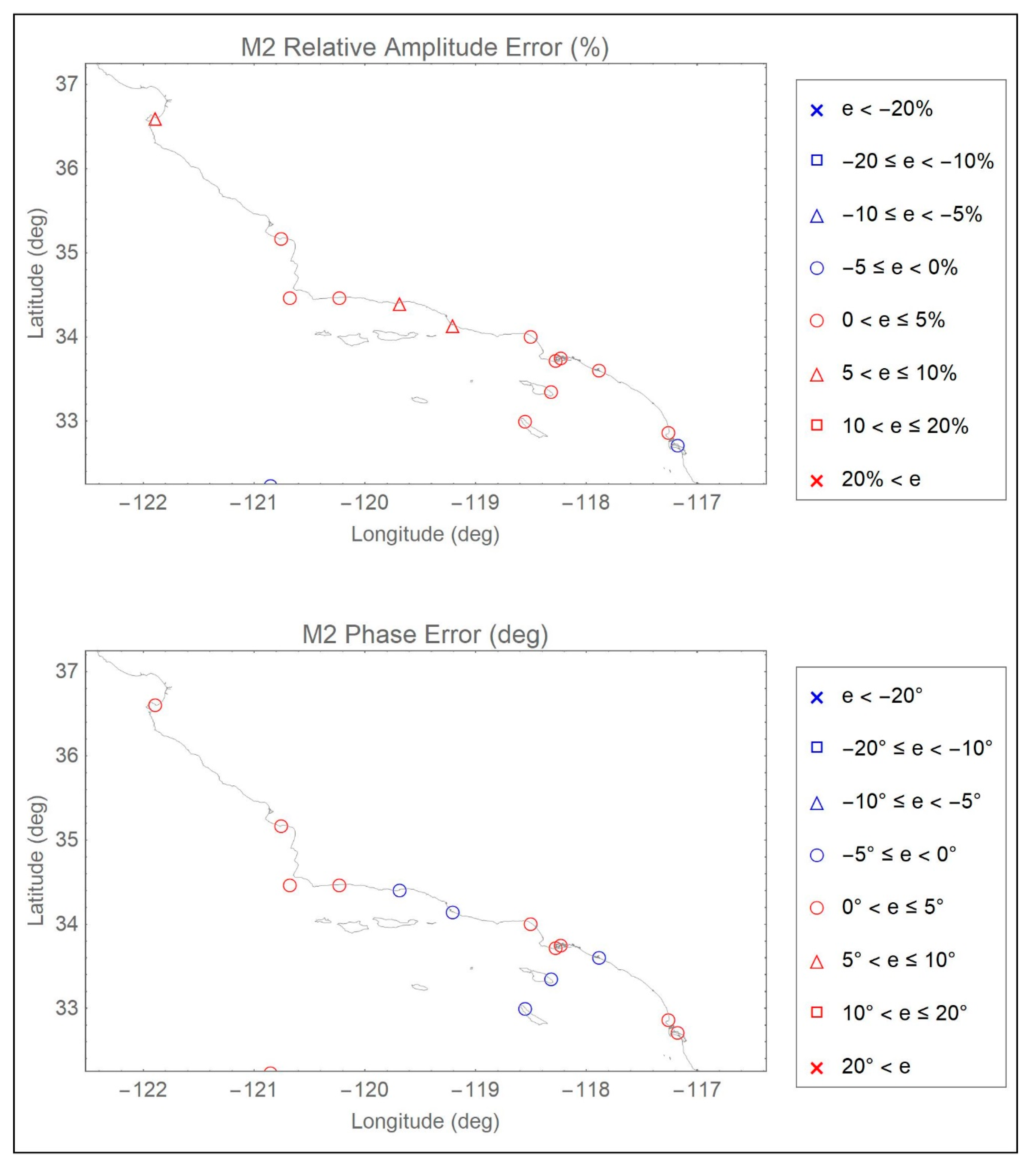
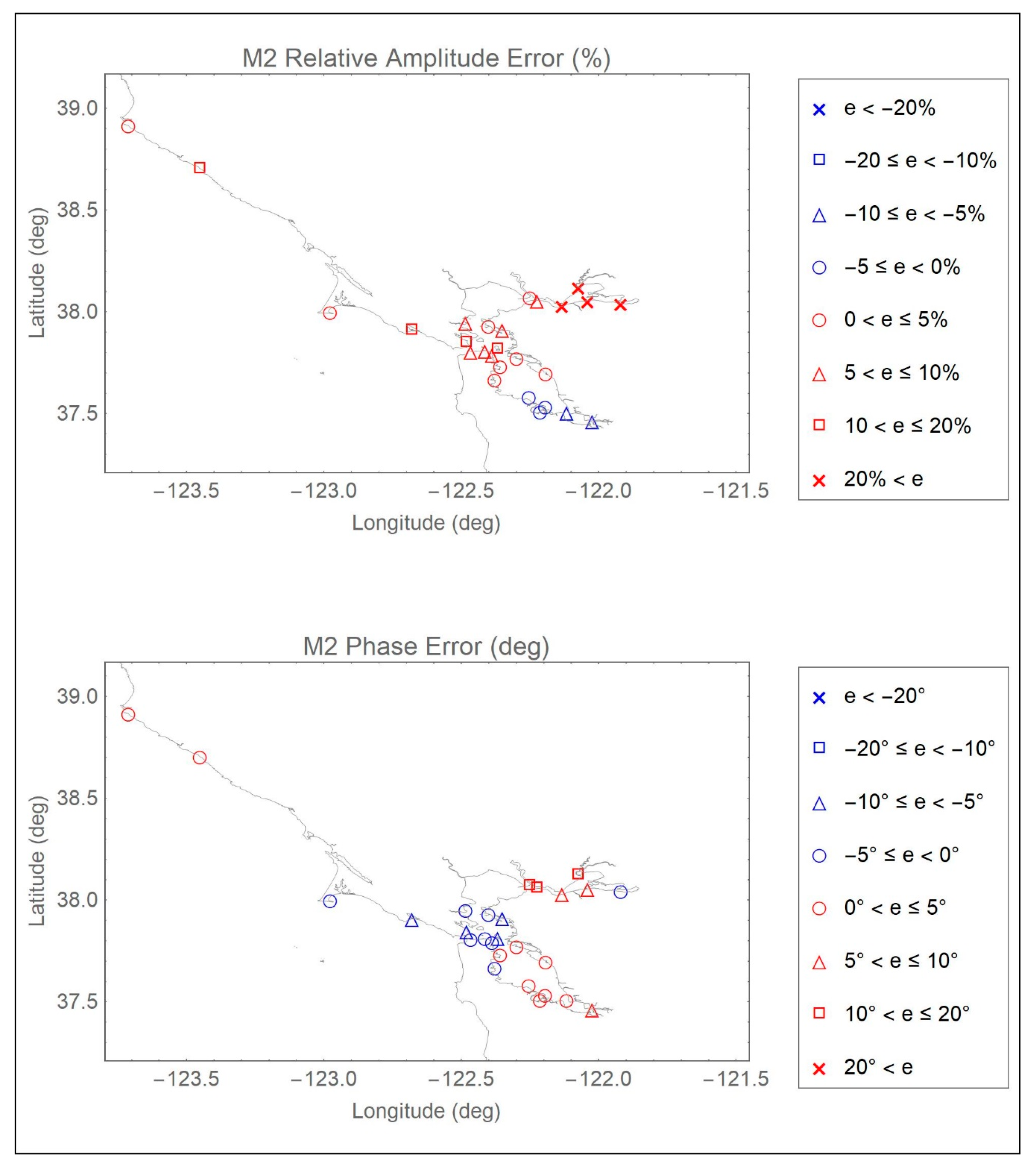
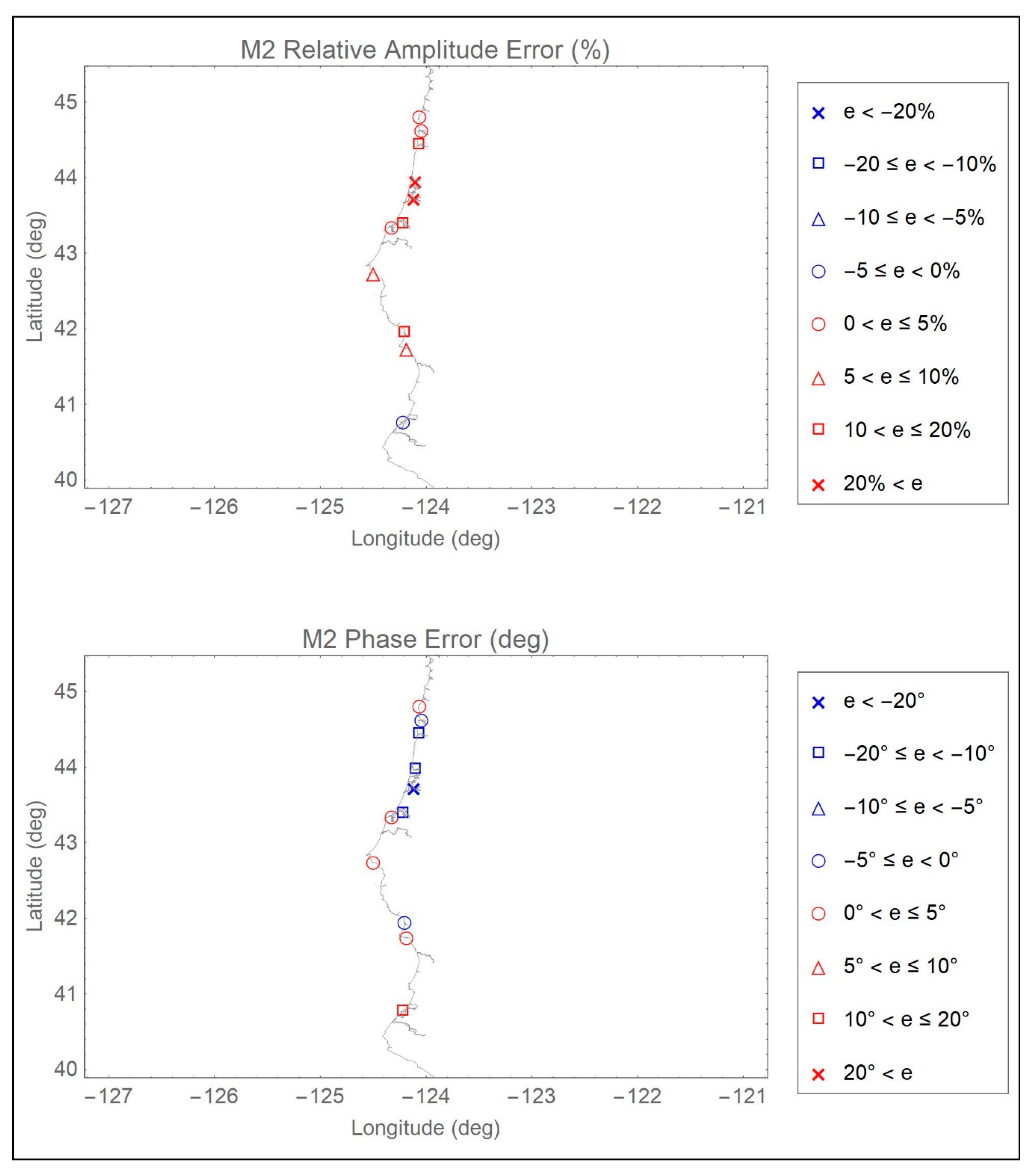
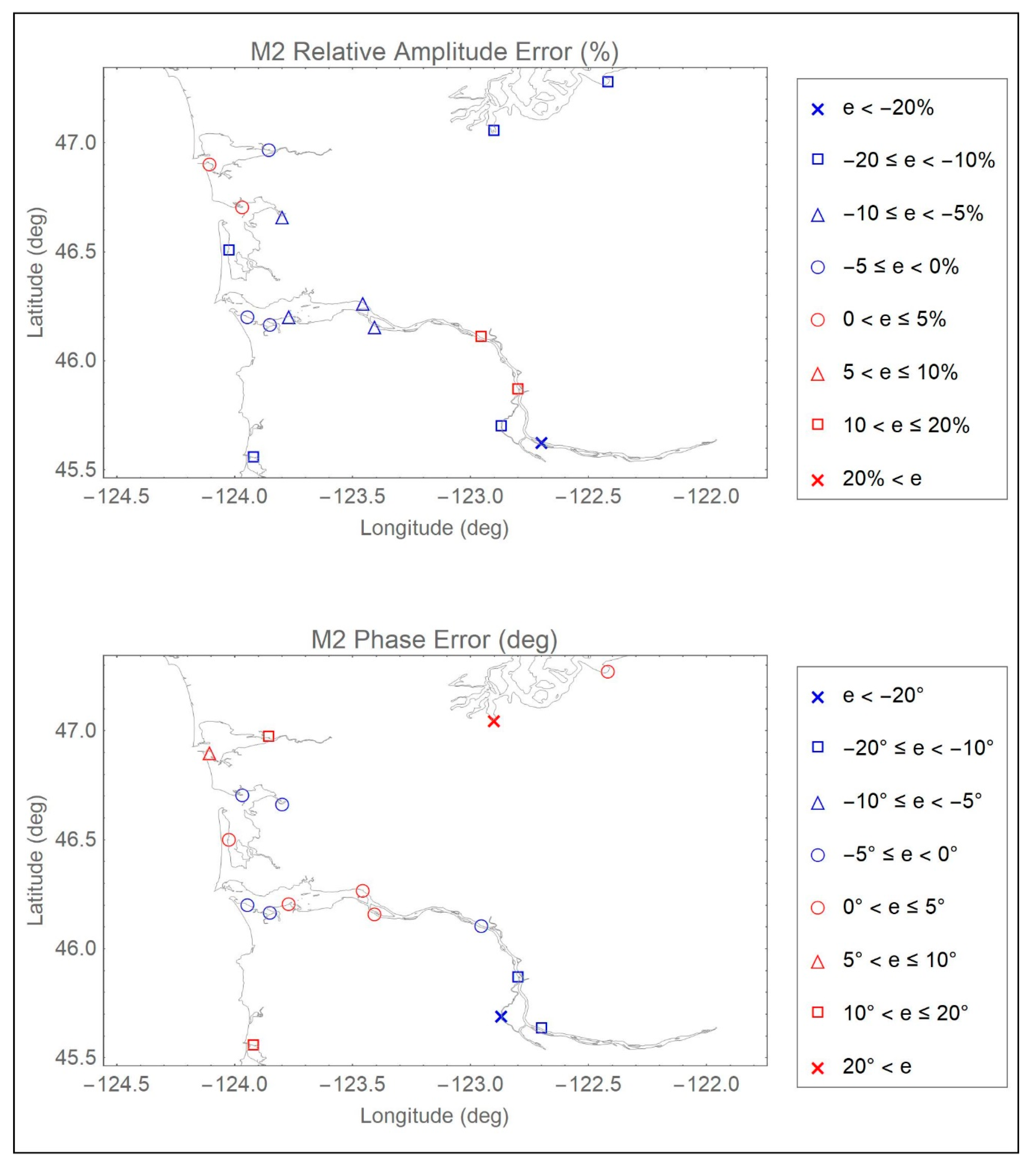
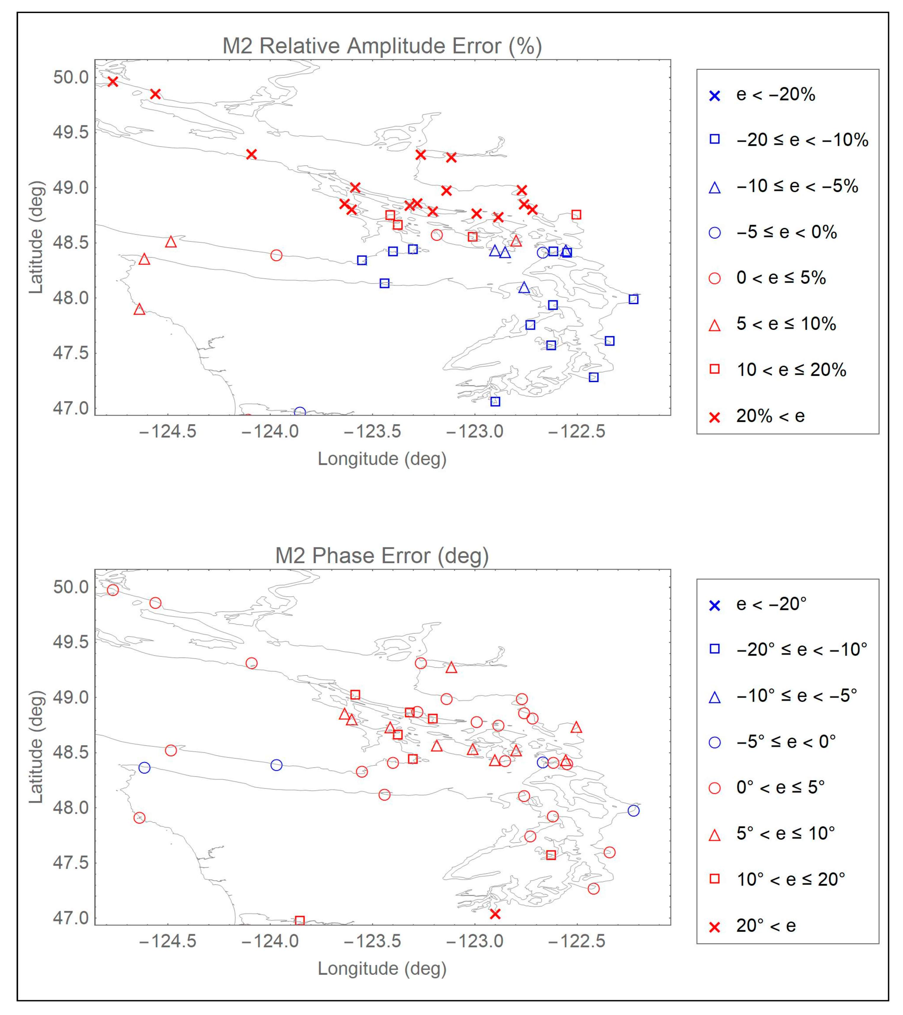
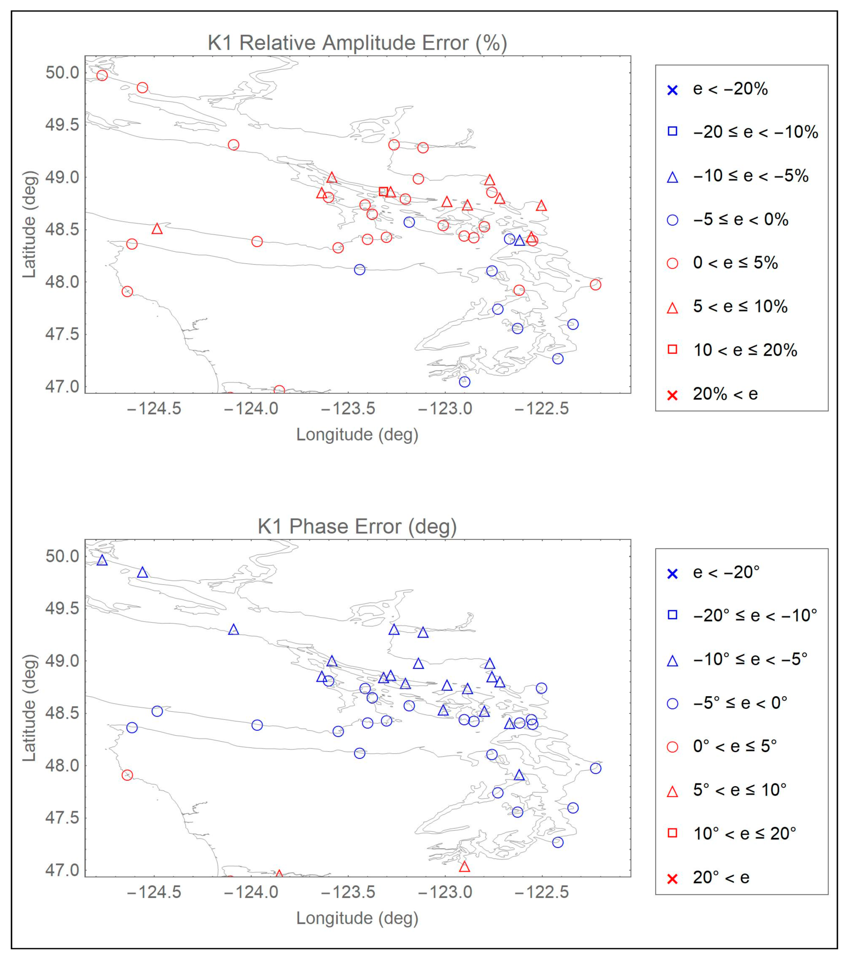
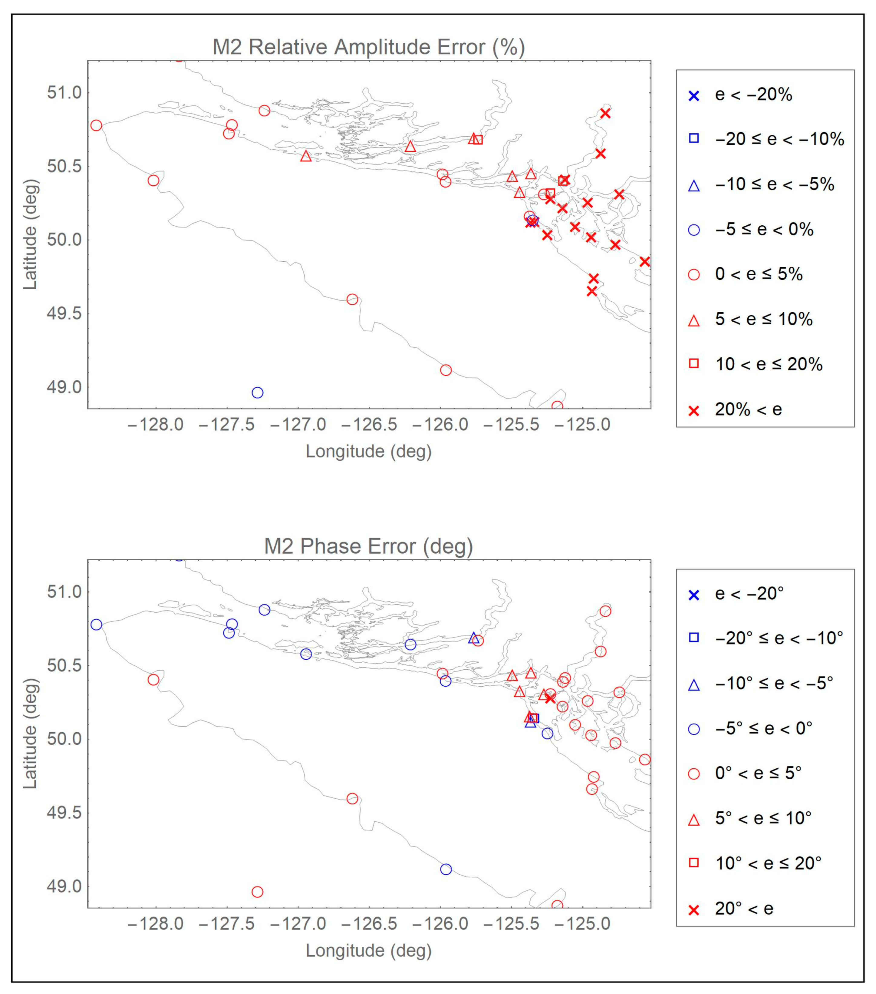
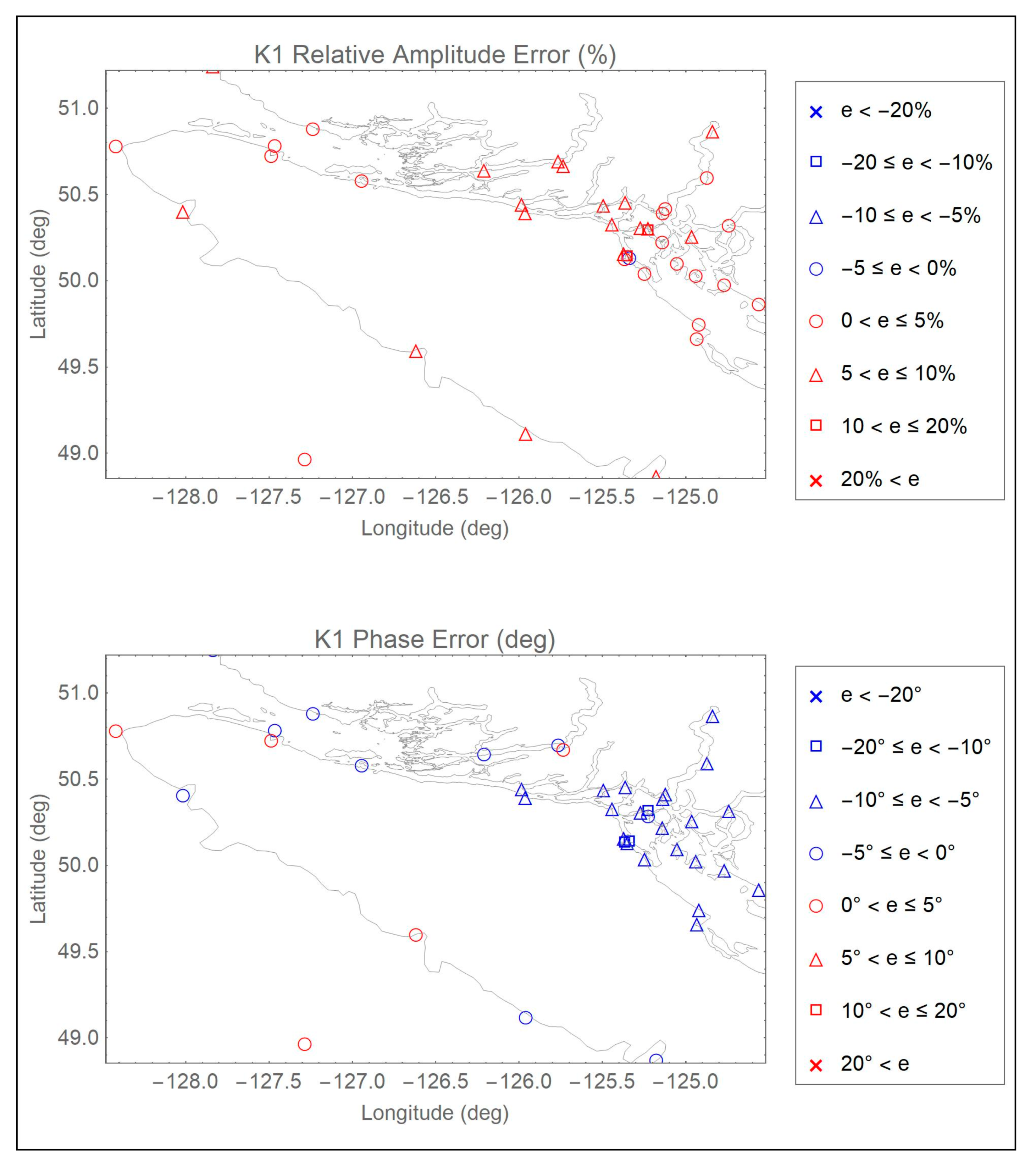
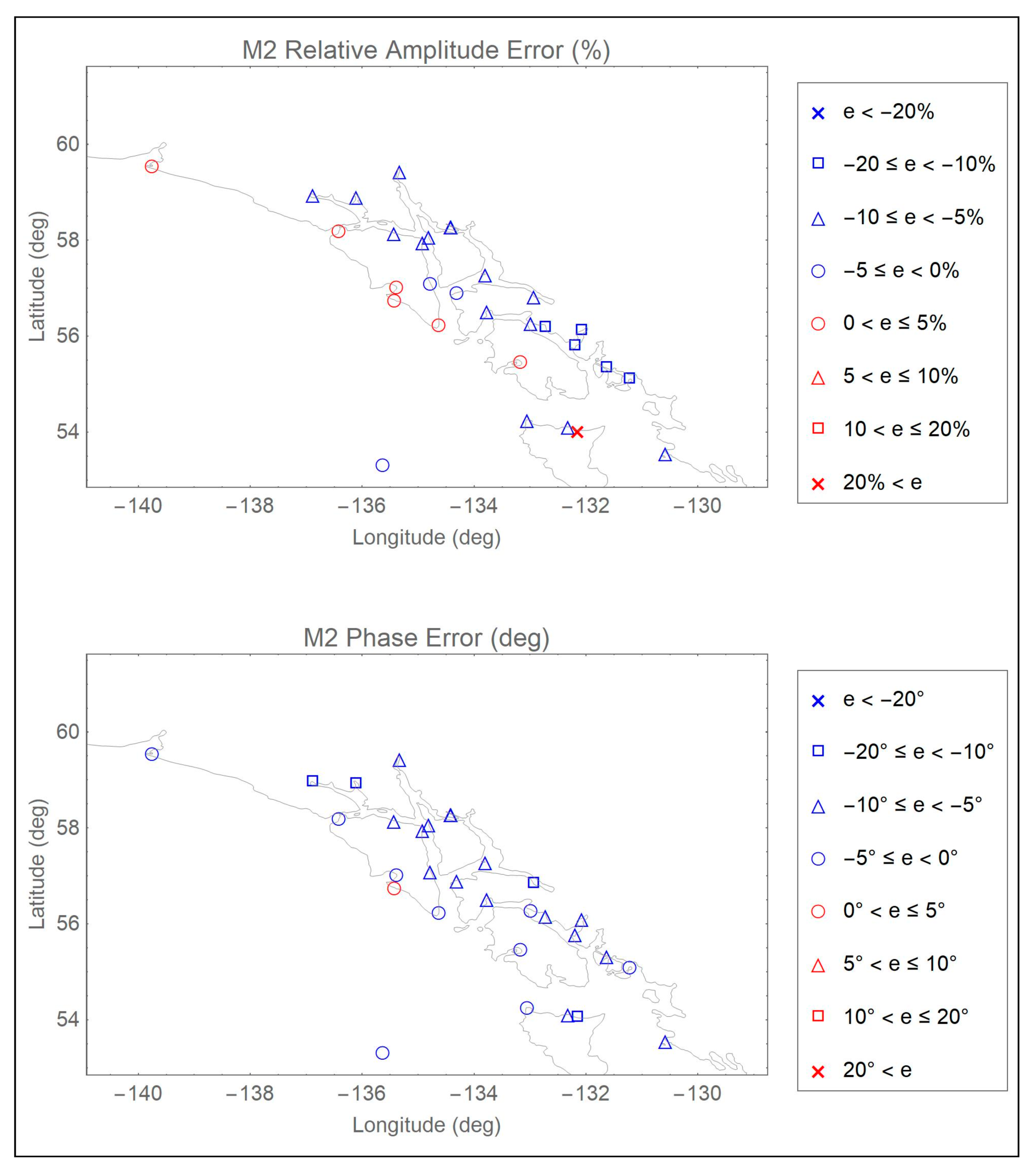
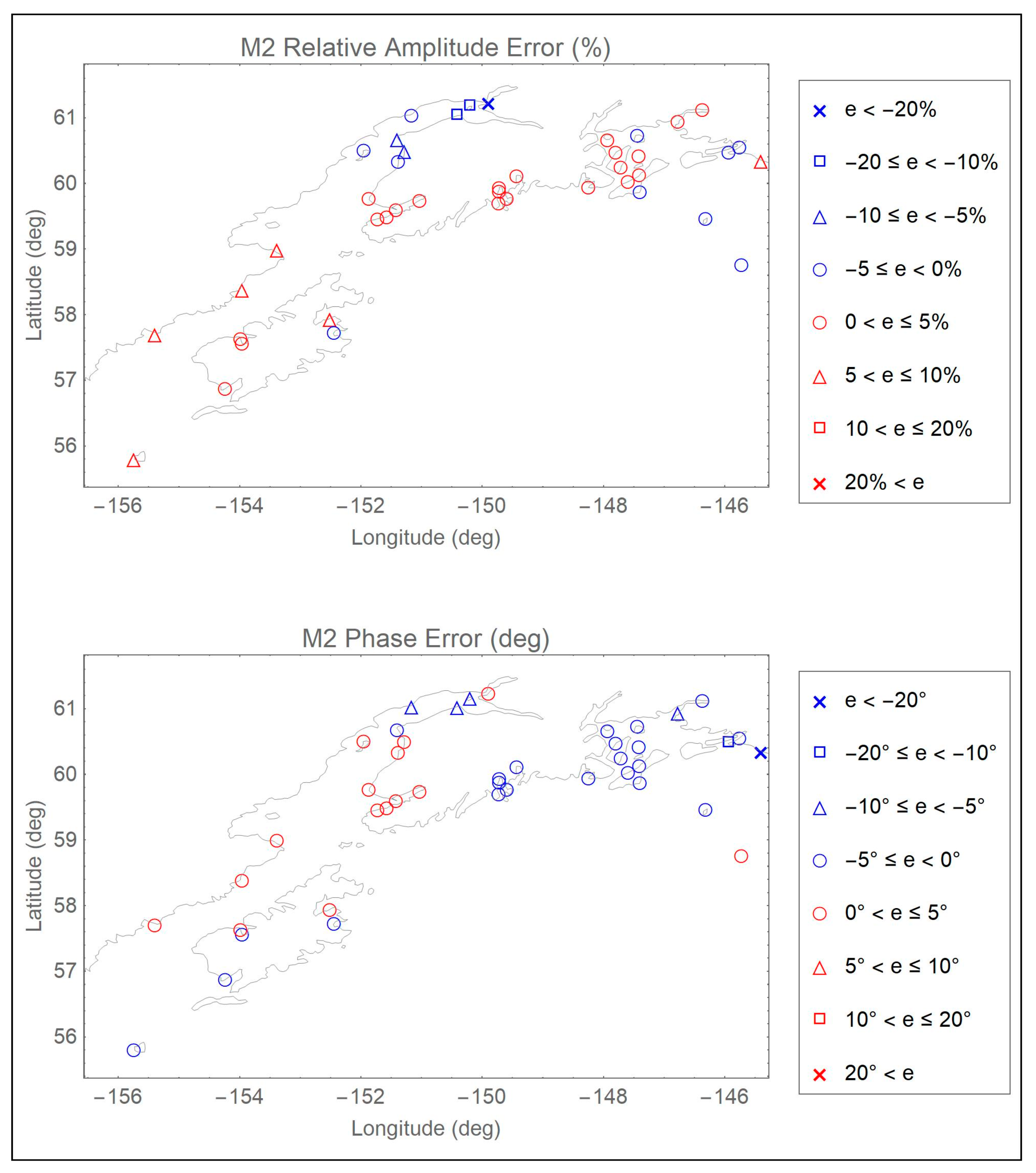
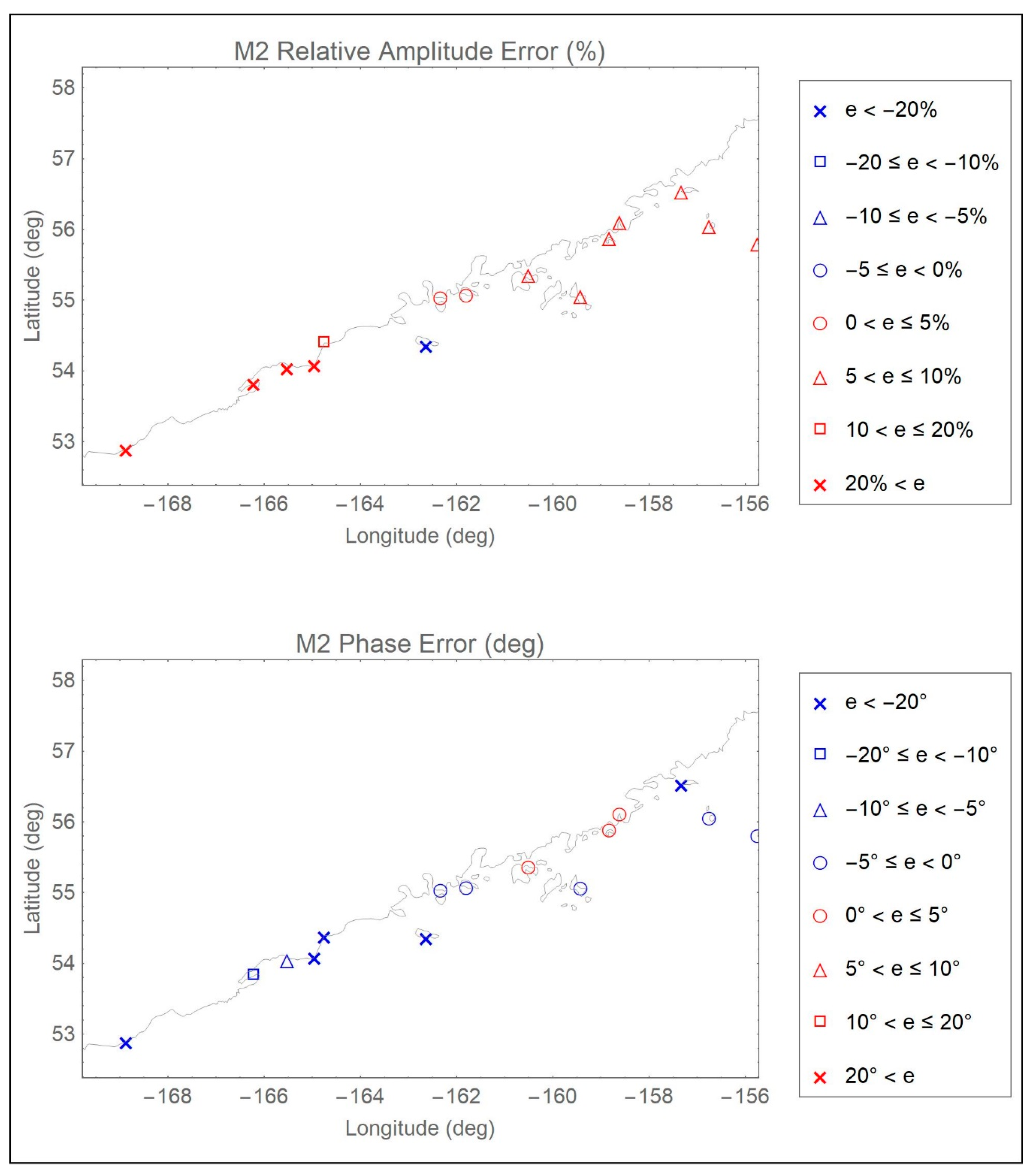
Finally, it is also instructive to see if there are sub-regional patterns in the errors (at the individual water body scale), which can help to guide future efforts at improving the tidal database. Plots of relative amplitude and absolute phase errors for the dominant M2 constituent at each of the 258 stations are provided for the global domain for the ENPAC15 model in Figure 10 in the text, while zoomed views of the smaller sub-regions are provided in Figure A15, Figure A16, Figure A17, Figure A18, Figure A19, Figure A20, Figure A21, Figure A22, Figure A23, Figure A24 and Figure A25 in Appendix D (the same zoom views given in Appendix A). For this study area, the M2 constituent is dominant for all regions except the inside passages north of Vancouver Island and Puget Sound, where the K1 constituent is of similar magnitude in some areas. Therefore, error plots for the K1 constituent are also provided for the Puget Sound sub region (Figure A20) and the Vancouver Island sub region (Figure A22). Points shown in blue are underestimating the amplitudes (or exhibit a phase lag), while points shown in red are overestimating (exhibit a phase lead). The symbol shapes indicate to what degree the model is over/under estimating; we would like to see amplitude errors less than 10% and phase errors less than 20°. Unless specifically noted, all subsequent comments refer to the M2 constituent. Several general trends can be gleaned from these plots.
- For Southern California, the ENPAC15 database is slightly overestimating the amplitude (generally within 5%) and phases are within ±5° from the data. Meanwhile, in San Francisco Bay, the database is more significantly overestimating the amplitudes, with the exception of the lower bay are where the data is underestimated; and the phases are generally within ±5° to 10°. This indicates the need to verify the bathymetry in this area and try a variable friction representation. Finally, along the Northern California coast, the amplitudes are overestimated by a more significant amount (over 20% for some stations), but the phases are generally within ±5°.
- Along the Oregon and Washington coast, generally, the amplitudes are underestimated and the phases are within ±5°. However, the further upriver stations in the Columbia River have higher errors, which may be indicative of the boundary being placed within the tidally influenced zone that is not being captured with the boundary condition at the end of the river, as well as the lack of freshwater inflow at the boundary.
- In the Puget Sound region, it is interesting that the M2 amplitudes are significantly overestimated (greater than 20%) in the channels heading east above Vancouver Island but are underestimated by 5–10% in the lower Puget Sound region; meanwhile, the phases exhibit a lead throughout much of this region (ranging from 5–20°). While the K1 amplitudes exhibit the same over/under regional trend, they are generally within 5% of the data; however, the phases exhibit a more conservative lag (5–10°) instead of a lead as compared to M2 constituent. Similarly in the Canadian waters above Vancouver Island, the M2 constituent is significantly overestimated (greater than 20%) in the interior passages but is more conservatively overestimated (0–10%) as you enter Queen Charlotte Strait to the east, while the interior passages exhibit slight phase leads and the easternmost parts of the channels slight phase lags (±5°). Meanwhile, the K1 constituent exhibits moderate amplitude overestimation of 0–10% and phase lags of 0–10°. For the region above Vancouver Island, it is important to note that the freshwater riverine flow can be significant in many of these channels, but it is neglected in our model. This neglegance has an impact on the accuracy of the tidal signal as you progress further up the channels.
- Along the southeast coast of Alaska, the amplitudes are underestimated by 5–20% in the interior passages and slightly overestimated (less than 5%) on the exterior coast, while the phases exhibit lags from 5 to 20°. Meanwhile, along the southern Alaskan coast, there is generally very good agreement for both amplitudes and phases (within ±5% or 5°), with the exception of the upper reaches of Cook Inlet, where amplitudes are underestimated up to 20%. Recall that the entire Alaskan coast received only minor bathymetric and coastline alignment updates, so we would not expect significant improvements. As you progress further west along the coast (past about 153° W), the amplitudes are more severely overestimated starting at 5% and going above 20% as you approach the boundary of the model, but the phase remains in good agreement until you pass 162° W. Recall that the coastline past Unimak Island is defined by a mainland boundary condition and does not include the interaction with the Bering Sea through the Aleutian Islands; therefore, we would not expect good agreement past 165° W.
4. Discussion
Table 8 provides a summary of the global RMS errors for the eight primary constituents, as well as the mean regional errors summed over these constituents (graphically presented in Figure 7), for each of the eight model simulations done as part of this study (statistics computed using only the 165 common validation data points). Returning to the six improvements (presented in Section 2.2) that were implemented to meet the objective of reducing the errors realized in the ENPAC03 database, we note the following:
- The placement of the open ocean boundary itself results in significant improvements for all regions (ENPAC03R vs. ESTOFS-trim1): global improvement of 33%. As was seen in previous databases for the ENPAC region, the location of the open ocean boundary can have significant impact on the accuracy of the interior model. However, as the ESTOFS-trim model incorporates newer bathymetry and has different resolution throughout, it is impossible to separate the effects of boundary placement, coarser mesh resolution at the boundary and updated deep water bathymetry when determining the source of these noted improvements.
- The improvements in coastal resolution (ESTOFS-trim1 vs. ENPAC15-CF) result in significant reductions in error for the Pacific Northwest region (38%), but no measurable change in the Alaska and California regions: global reduction of 22%. Recall that the coast of Alaska was not updated, as the VDatum project for that region is still ongoing. Furthermore, examination of individual station scatterplots for the California region indicate that some significant improvements are realized in the San Francisco Bay area but not in the open ocean coastal stations. The Pacific Northwest improvements are most likely attributable to the inclusion of the passages north of Vancouver Island.
- Meanwhile, the updated boundary forcing (ENPAC03 vs. ENPAC03R) slightly increases the mean RMS errors for some constituents (K1, M2) while decreasing others (S2 and K2). Comparison of the along boundary forcing values applied from the TPXO6 and TPXO8 products indicate only minor changes in amplitudes and no changes in applied phases near the westernmost ocean boundary (near Alaska) and no changes elsewhere. Therefore, the changes between the resulting harmonics are more than likely due to the addition of the long-term constituents in the forcing suite; recall that the ENPAC database was only forced with the diurnal and semi-diurnal constituents. However, there is very little change noted when results are compared for the TPXO8 (ESTOFS-trim1) and FES12 (ESTOFS-trim6) forcing.
- In general, the use of a variable bottom friction scheme (ENPAC15-Mann) results in lower error metrics than when a constant value is used (ENPAC15-CF), for all constituents and regions. However, the same effect can also be attained by using a slightly higher constant value (ENPAC15-Vdat). Therefore, more work needs to be done in determining appropriate variable values and comparing scatterplots by station instead of just regionally, in order to decide which scheme is best. Ideally, each sub region would be carefully calibrated taking into consideration actual bed formations and sea bed materials.
- The inclusion of the advective terms in the governing equations (ESTOFS-trim1 vs. ESTOFS-trim2), most notably, results in improvements in the Pacific Northwest region (14%) and particularly the M2 and K1 constituents. This is to be expected as the passages north of Vancouver Island are known to dissipate a great deal of internal energy. Further work must be done to stabilize these passages so that the advective terms can be utilized in the next tidal database release.
- The overall error reductions due to the combined effects of all five improvements (no advection) that were used in the latest database (ENPAC15-VDat vs. ENPAC03) are as follows: the global errors are reduced by 52%; while the regional errors are reduced by 33% in Alaska, 68% in the Pacific Northwest and 45% in California. Users of ENPAC15 can expect greater accuracy in any localized region where they apply boundary conditions, but particularly in the Pacific Northwest.
These results indicate that most of the reduction in harmonic constituent errors are due to the increased coastal resolution and updated bathymetry, as well as the actual placement of the boundary itself. Furthermore, the addition of the advective terms would improve the results in the Pacific Northwest region, if the model was to remain stable. On average, very little overall improvement was realized solely from the bottom friction representation; however, the friction contributes to localized effects on the harmonic accuracy and it is important to have an accurate representation of the bottom friction in the shallower regions. Finally, the updated ocean boundary forcing does not have a large effect on the overall accuracy.
To put these errors in context, the mean RMS error (summed over all eight primary constituents) between the three data sets (CO-OPS, IOS-FOC and IHO) was computed at the 61 stations that were duplicated in any two data sets. The mean error for all 61 stations was 1.1 cm, while the minimum and maximum error over all stations were 0.01 cm and 7.6 cm, respectively. Therefore, on average, one could expect the data itself to be in error by about 1 cm at a given station, which accounts for about 20% of the global RMS errors reported for the ENPAC03 model in Table 8, about 30% of the ESTOFS-trim models and 40% of the error for the ENPAC15 models. The error measures reported throughout the paper include these errors in the data; thus, a significant portion of the reported errors may stem from the uncertainty in the data itself.
Future improvements to the ENPAC tidal database should include updated resolution and bathymetry for the Alaskan coastal waters and could include better bottom friction representations in individual water bodies that have not been optimized (e.g., San Francisco Bay, Puget Sound, the inside passages north of Vancouver Island and in southeast Alaska and Cook Inlet). Additionally, for the database to be valid west of the old ENPAC03 model domain, a more accurate representation of the Aleutian Island chain and the connection to the Bering Sea would be necessary. It could also be informative to use a mesh with coarser coastal resolution, such as ESTOFS-trim, to further explore the effects of boundary location on the accuracy of the tidal harmonics.
It is important to note that the simulation used to compute the ENPAC15 database does not include all physical processes which can affect the model response including (but not limited to) density driven flows, riverine discharge, sediment transport and resulting bed morphological changes, large-scale oceanic currents or wind and atmospheric pressure driven flows. To minimize the effects of these limitations, it is recommended that users of the ENPAC15 tidal database follow three basic guidelines: (1) choose your regional open ocean boundary location to be well outside of estuaries and bays; (2) make sure that your regional model bathymetry matches the database bathymetry at your boundary and (3) do not extract any data west of the old ENPAC03 model domain (near 160° W) as the Aleutian Island chain is treated as a mainland boundary and results are not accurate past this point. Additionally, while harmonic information is available for 37 constituents, use caution when applying larger suites as only eight have been validated. For the interested reader, further guidelines and limitations are provided in Appendix E. The ENPAC15 tidal database is available on the ADCIRC website [59].
Author Contributions
Conceptualization, R.K. and T.C.M.; Data Curation, C.S.; Formal Analysis, C.S.; Funding Acquisition, T.C.M.; Investigation, C.S.; Methodology, C.S.; Project Administration, R.K.; Resources, R.K. and T.C.M.; Software, C.S. and K.D.; Supervision, K.D. and T.C.M.; Validation, C.S.; Visualization, C.S.; Writing—Original Draft, C.S.; Writing—Review and Editing, C.S., K.D., R.K. and T.C.M.
Funding
This research was funded by the Institute of Water Resources and the Engineer Research and Development Center|U.S. Army Corps of Engineers BAA 12-5008 under contract W912HZ-13-P-0046. Additional resources were provided by the University of Oklahoma. Any opinions, conclusions, or findings are those of the authors and are not necessarily endorsed by the funding agencies.
Acknowledgments
The computing for this project was performed at the OU Supercomputing Center for Education and Research (OSCER) at the University of Oklahoma (OU). The authors would also like to acknowledge Mike Foreman at IOS-FOC for providing model domains and validation data for the areas covering British Columbia, as well as Pete Bacopoulos for creating the LTEA mesh for the Vancouver Island region. Finally, the authors acknowledge the assistance of Jiangtao Xu, Edward Myers and Jesse Feyen (among others) at NOAA for providing a summary of harmonic validation data for all stations currently covered by CO-OPS, VDatum models and input files for the US West Coast, the ESTOFS-Pacific operational mesh for the West Coast of the United States, and for assisting in extracting input data from the FES12 global database. Figure 1, Figure 2, Figure 3, Figure 4, Figure 5, and Figure 6 were generated using a modified version of FigureGen [14]. The authors also thank the reviewers for providing constructive comments to improve the presentation of the paper.
Conflicts of Interest
The authors declare no conflict of interest. T.M. as a representative of the funding sponsor was involved in designing the study and reviewing the final product. The funders had no role in the collection, analyses, or interpretation of data; in the writing of the manuscript; or in the decision to publish the results.
Appendix A
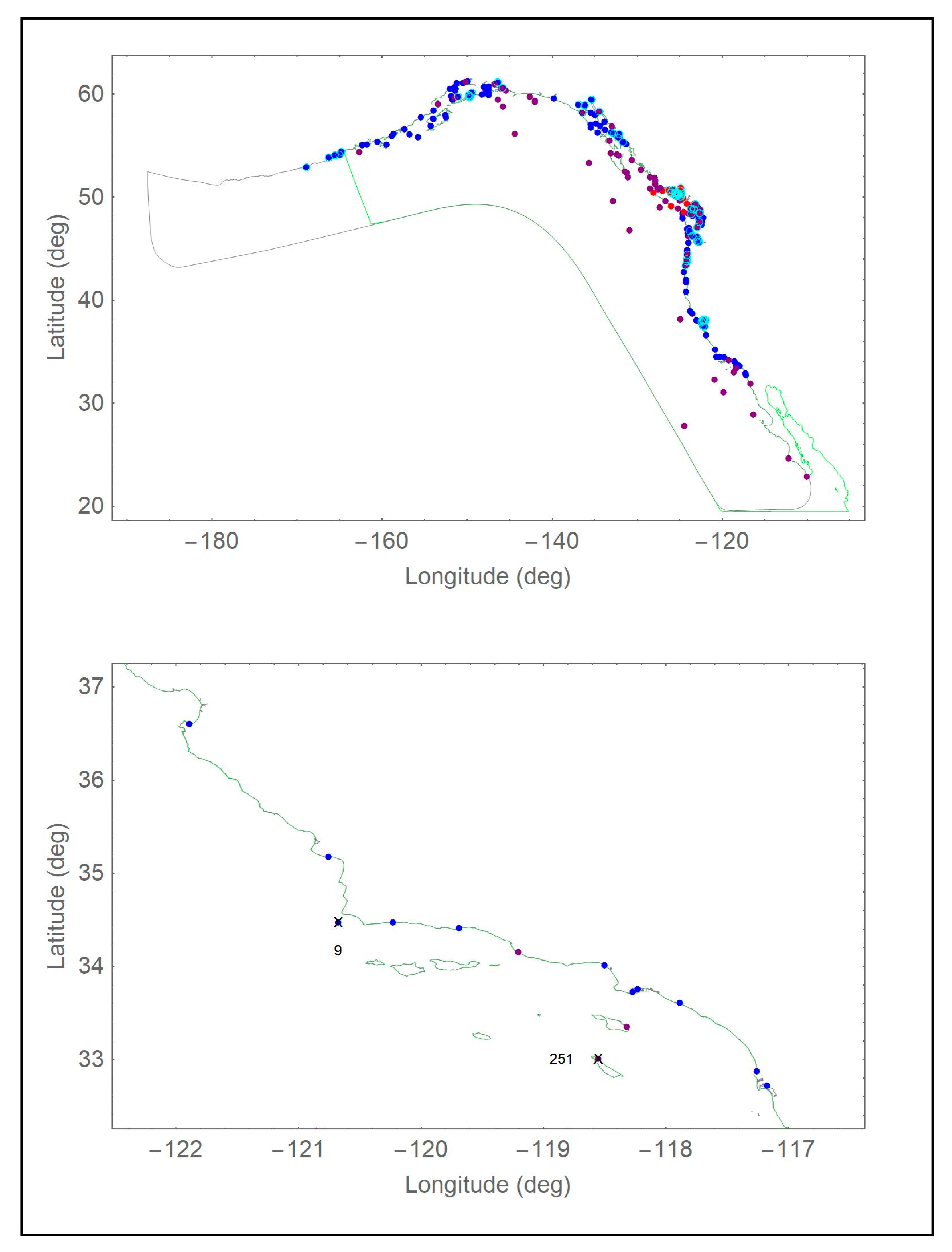
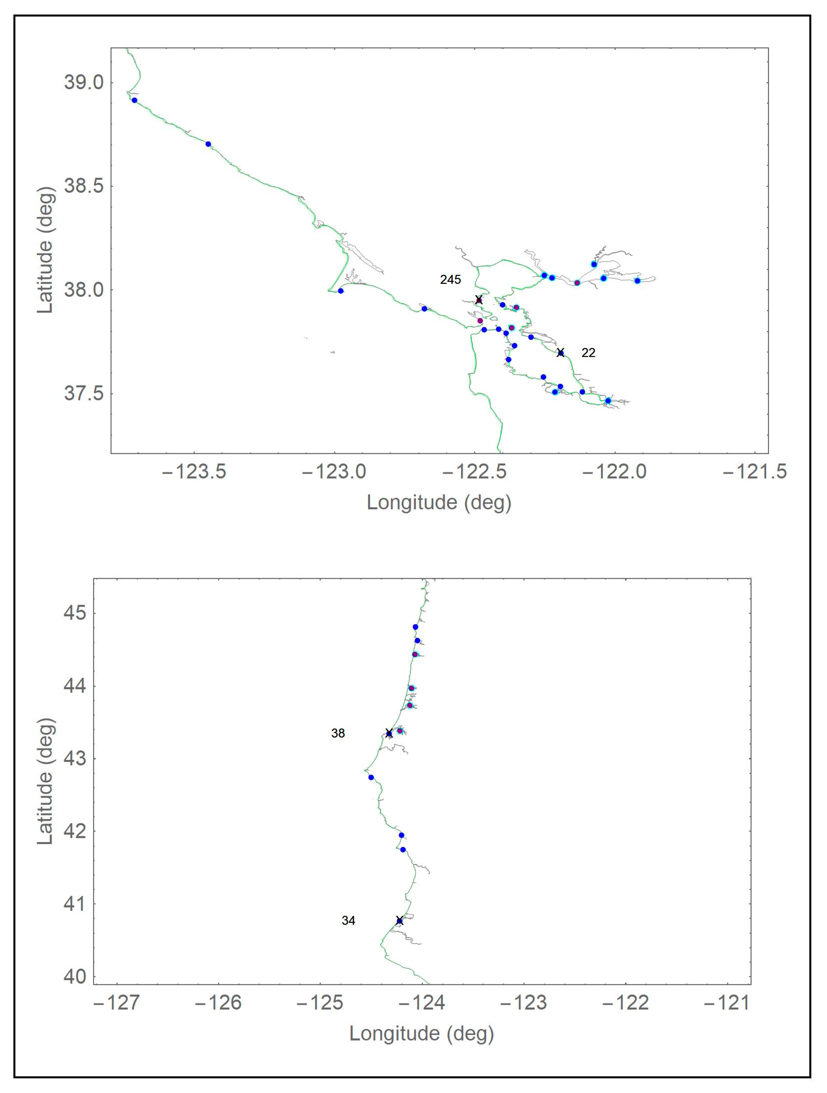
The locations of the 258 validation stations are plotted with the model domain boundaries shown for the ENPAC03 (green) and ENPAC15 (gray) databases. Each figure in this Appendix zooms into a specific sub-region of the ENPAC domain in order to show the details of the coastline near the stations. Stations indicated with a black X designate those which scatter plots are provided for in Appendix C and the numbers correspond to the list of stations provided in Appendix B. The three data sources are indicated by color as follows: CO-OPS in blue, IOS-FOC in red and IHO in magenta. Furthermore, those stations that are dry in the ENPAC03 database, and will not be used for comparison with other models, are indicated with a cyan circle around the station point.
Figure A1.
Location of validation stations: global and Southern California.

Figure A2.
Location of validation stations: San Francisco Bay and Northern California.

Figure A3.
Location of validation stations: Columbia River and Puget Sound.

Figure A4.
Location of validation stations: British Columbia and Southeast Alaska.

Figure A5.
Location of validation stations: South Alaska.

Appendix B
The locations, names and regional classification of all 258 validation stations are given herein. For the first 139 stations, the official CO-OPS station number is provided in the source designation column, while IOS-FOC is used to designate those stations from the Institute of Ocean Sciences—Fisheries and Oceans Canada and IHO to designate the historical stations from the International Hydrographic Organization. Stations marked with a single asterisk are considered wet in the ENPAC03 model even though they are approximated by their nearest neighbor (actual longitude and latitude coordinates were not shifted when extracting from the ENPAC03 database, as the nearest element is most likely where the station would have been manually shifted anyway). Meanwhile, those marked with a double asterisk are not included in scatter plots or statistical error metrics for the ENPAC03 database since they are well outside the domain of the boundary or are in channels and other features that are not represented in the ENPAC03 model domain. Abbreviations for the region designations are as follows: Alaska—AK, British Columbia—BC, Washington—WA, Oregon—OR, California—CA, Mexico—MX, and deep water—D. Note that for statistics, the British Columbia, Washington and Oregon stations were grouped into a single Pacific Northwest category; however, they are listed separately for interested readers. Similarly, the California and Mexico stations were grouped into a single category for statistical analysis.

Table A1.
Location and source information for validation data. For the first 139 stations, the number in the Source column is the CO-OPS station identifier.
Table A1.
Location and source information for validation data. For the first 139 stations, the number in the Source column is the CO-OPS station identifier.
| Station | Longitude | Latitude | Station Name | Region | Source |
|---|---|---|---|---|---|
| 1 * | −117.17360 | 32.71400 | San Diego, San Diego Bay | CA | 9410170 |
| 2 | −117.25800 | 32.86670 | La Jolla, Pacific Ocean | CA | 9410230 |
| 3 * | −117.88300 | 33.60330 | Newport Beach, Newport Bay Ent | CA | 9410580 |
| 4 * | −118.27200 | 33.72000 | Los Angeles, Outer Harbor | CA | 9410660 |
| 5 * | −118.22700 | 33.75170 | Long Beach, Terminal Island | CA | 9410680 |
| 6 * | −118.50000 | 34.00830 | Santa Monica, Pacific Ocean | CA | 9410840 |
| 7 | −119.68501 | 34.40830 | Santa Barbara, Pacific Ocean | CA | 9411340 |
| 8 * | −120.22831 | 34.46939 | Gaviota State Park, Pacific Ocean | CA | 9411399 |
| 9 | −120.67300 | 34.46830 | Oil Platform Harvest (Topex) | CA | 9411406 |
| 10 * | −120.76000 | 35.17670 | Port San Luis, San Luis Obispo | CA | 9412110 |
| 11 * | −121.88800 | 36.60500 | Monterey, Monterey Harbor | CA | 9413450 |
| 12 * | −122.46500 | 37.80669 | San Francisco, San Francisco Bay | CA | 9414290 |
| 13 * | −122.41300 | 37.81000 | North Point [Pier 41] S.F.Bay | CA | 9414305 |
| 14 * | −122.38698 | 37.79002 | Pier 22 1/2, San Francisco Bay | CA | 9414317 |
| 15 | −122.35700 | 37.73000 | Hunters Point, S.F. Bay | CA | 9414358 |
| 16 | −122.37700 | 37.66500 | Oyster Point Marina, S.F. Bay | CA | 9414392 |
| 17 | −122.25300 | 37.58000 | San Mateo Bridge, West Side | CA | 9414458 |
| 18 | −122.19300 | 37.53330 | Redwood Creek, C.M. No. 8,S.F.B | CA | 9414501 |
| 19 | −122.11500 | 37.50670 | Dumbarton Bridge, S. F. Bay | CA | 9414509 |
| 20 ** | −122.21200 | 37.50670 | Redwood City, Wharf 5, S.F. Bay | CA | 9414523 |
| 21 ** | −122.02300 | 37.46500 | Coyote Creek, Alviso Slough | CA | 9414575 |
| 22 * | −122.19200 | 37.69500 | San Leandro Marina, S.F.Bay | CA | 9414688 |
| 23 | −122.29833 | 37.77167 | Alameda, San Francisco Bay | CA | 9414750 |
| 24 | −122.40000 | 37.92830 | Richmond, Chevron Oil Pier | CA | 9414863 |
| 25 ** | −121.91800 | 38.04330 | Mallard Island, Suisun Bay | CA | 9415112 |
| 26 ** | −122.22300 | 38.05830 | Crockett, Carquinez Strait | CA | 9415143 |
| 27 ** | −122.03950 | 38.05600 | Port Chicago, Suisun Bay | CA | 9415144 |
| 28 ** | −122.25000 | 38.07000 | Mare Is.Naval Shipyard, Carquin | CA | 9415218 |
| 29 ** | −122.07300 | 38.12323 | Suisun Slough Entrance | CA | 9415265 |
| 30 * | −122.67854 | 37.90871 | Bolinas, Bolinas Lagoon | CA | 9414958 |
| 31 * | −122.97670 | 37.99610 | Point Reyes, Drakes Bay | CA | 9415020 |
| 32 | −123.44940 | 38.70329 | Green Cove, Pacific Ocean | CA | 9416409 |
| 33 * | −123.71061 | 38.91330 | Arena Cove, Pacific Ocean | CA | 9416841 |
| 34 * | −124.21700 | 40.76670 | North Spit, Humboldt Bay | CA | 9418767 |
| 35 | −124.18300 | 41.74500 | Crescent City, Pacific Ocean | CA | 9419750 |
| 36 * | −124.20092 | 41.94525 | Pyramid Point, Smith River | CA | 9419945 |
| 37 | −124.49828 | 42.73897 | Port Orford, Pacific Ocean | OR | 9431647 |
| 38 * | −124.32200 | 43.34500 | Charleston, Coos Bay | OR | 9432780 |
| 39 * | −124.04300 | 44.62500 | South Beach, Yaquina River | OR | 9435380 |
| 40 * | −124.06300 | 44.81000 | Depoe Bay | OR | 9435827 |
| 41 * | −123.91894 | 45.55453 | Garibaldi, Tillamook Bay | OR | 9437540 |
| 42 * | −123.94500 | 46.20170 | Hammond, Columbia River | OR | 9439011 |
| 43 * | −123.76831 | 46.20731 | Astoria, Tongue Point, Columbia | OR | 9439040 |
| 44 ** | −123.40500 | 46.16000 | Wauna, Columbia River | OR | 9439099 |
| 45 ** | −122.86800 | 45.69670 | Rocky Point, Multnomah Channel | OR | 9439189 |
| 46 ** | −122.79700 | 45.86500 | St. Helens, Columbia River | OR | 9439201 |
| 47 ** | −122.69704 | 45.63158 | Vancouver, Columbia River | WA | 9440083 |
| 48 ** | −122.95420 | 46.10559 | Longview, Columbia River | WA | 9440422 |
| 49 ** | −123.45602 | 46.26707 | Skamokawa, Columbia River | WA | 9440569 |
| 50 | −124.02300 | 46.50170 | Nahcotta, Willapa Bay | WA | 9440747 |
| 51 ** | −123.79800 | 46.66404 | South Bend | WA | 9440875 |
| 52 * | −123.96692 | 46.70746 | Toke Point, Willapa Bay | WA | 9440910 |
| 53 * | −124.10508 | 46.90431 | Westport, Grays Harbor | WA | 9441102 |
| 54 * | −123.85300 | 46.96830 | Aberdeen, Grays Harbor | WA | 9441187 |
| 55 * | −124.63700 | 47.91330 | La Push, Quillayute River | WA | 9442396 |
| 56 | −124.61170 | 48.37081 | Neah Bay, Strait of Juan De Fuca | WA | 9443090 |
| 57 * | −123.44000 | 48.12500 | Port Angeles, Juan De Fuca | WA | 9444090 |
| 58 | −122.75800 | 48.11170 | Port Townsend, Admiralty Inlet | WA | 9444900 |
| 59 | −122.61700 | 47.92670 | Foulweather Bluff, Twin Spits | WA | 9445016 |
| 60 * | −122.72700 | 47.74830 | Bangor | WA | 9445133 |
| 61 * | −122.41670 | 47.27120 | Tacoma, Commencement Bay | WA | 9446484 |
| 62 * | −122.33931 | 47.60264 | Seattle, Puget Sound | WA | 9447130 |
| 63 * | −122.22300 | 47.98000 | Everett | WA | 9447659 |
| 64 | −122.54800 | 48.40000 | Sneeoosh Point, Skagit Bay | WA | 9448576 |
| 65 ** | −122.55500 | 48.44500 | Turner Bay, Similk Bay | WA | 9448657 |
| 66 | −122.75800 | 48.86330 | Cherry Point, Strait of Georgia | WA | 9449424 |
| 67 * | −122.76900 | 48.99227 | Blaine, Drayton Harbor | WA | 9449679 |
| 68 * | −123.00980 | 48.54580 | Friday Harbor, San Juan Channel | WA | 9449880 |
| 69 * | −122.79700 | 48.53500 | Armitage Island | WA | 9449932 |
| 70 * | −122.90000 | 48.44670 | Richardson, Lopez Island | WA | 9449982 |
| 71 * | −131.21900 | 55.10280 | Custom House Cove, Mary Island | AK | 9450296 |
| 72 ** | −131.62619 | 55.33183 | Ketchikan, Tongass Narrows | AK | 9450460 |
| 73 ** | −132.19088 | 55.78828 | Magnetic Point, Union Bay | AK | 9450753 |
| 74 ** | −132.07650 | 56.11512 | Thoms Point, Zimovia Strait | AK | 9450970 |
| 75 ** | −132.71750 | 56.17830 | Point Harrington, Clarence Strait | AK | 9451005 |
| 76 ** | −132.98500 | 56.27670 | Bushy Island, Snow Passage | AK | 9451074 |
| 77 | −133.76610 | 56.52760 | Monte Carlo Island | AK | 9451247 |
| 78 | −134.62713 | 56.23934 | Port Alexander, Baranof Island | AK | 9451054 |
| 79 | −135.41829 | 56.75322 | Golf Island, Necker Islands | AK | 9451421 |
| 80 | −134.30400 | 56.90856 | Saginaw Bay, Kuiu Island | AK | 9451497 |
| 81 | −135.38450 | 57.03000 | Sitka, Baronof Island, Sitka Sound | AK | 9451600 |
| 82 | −134.77960 | 57.09860 | Baranof, Warm Spring Bay | AK | 9451625 |
| 83 * | −133.79700 | 57.29500 | The Brothers, Stephens Passage | AK | 9451785 |
| 84 ** | −134.41200 | 58.29818 | Juneau, Gastineau Channel | AK | 9452210 |
| 85 * | −134.80600 | 58.08410 | Hawk Inlet Entrance | AK | 9452294 |
| 86 | −134.91580 | 57.96780 | False Bay, Chatham Strait | AK | 9452328 |
| 87 ** | −135.32880 | 59.44960 | Skagway, Taiya Inlet | AK | 9452400 |
| 88 | −135.43190 | 58.15240 | Hoonah | AK | 9452438 |
| 89 ** | −136.10800 | 58.91330 | Muir Inlet, Glacier Bay | AK | 9452584 |
| 90 ** | −136.88110 | 58.95960 | Tarr Inlet | AK | 9452749 |
| 91 * | −139.74890 | 59.54850 | Yakutat, Yakutat Bay | AK | 9453220 |
| 92 ** | −145.75300 | 60.55830 | Cordova, Orca Inlet, Pr William Sd | AK | 9454050 |
| 93 ** | −146.36200 | 61.12360 | Valdez, Prince William Sound | AK | 9454240 |
| 94 | −147.40050 | 60.13250 | Perch Point, Montague Island | AK | 9454561 |
| 95 * | −147.39840 | 59.87220 | Wooded Island | AK | 9454562 |
| 96 | −147.41000 | 60.42500 | Seal Island | AK | 9454564 |
| 97 * | −147.43700 | 60.73670 | Storey Island North Side | AK | 9454571 |
| 98 | −147.59300 | 60.02800 | Montague Island, Ne Bazel Pt | AK | 9454616 |
| 99 * | −147.70950 | 60.24760 | Snug Harbor, Knight Island | AK | 9454662 |
| 100 * | −147.79270 | 60.47560 | Herring Point, Knight Island, | AK | 9454691 |
| 101 * | −147.93200 | 60.66910 | Perry Island (South Bay) | AK | 9454721 |
| 102 * | −148.24540 | 59.94370 | Point Erlington, Erlington Island | AK | 9454814 |
| 103 ** | −149.42667 | 60.12000 | Seward, Resurrection Bay | AK | 9455090 |
| 104 ** | −149.58630 | 59.77430 | Agnes Cove | AK | 9455120 |
| 105 ** | −149.71340 | 59.94060 | Aialik Bay, North End | AK | 9455145 |
| 106 ** | −149.71800 | 59.88500 | Aialik Sill, Aialik Bay | AK | 9455146 |
| 107 ** | −149.72500 | 59.70240 | Camp Cove, Harris Penninsula | AK | 9455151 |
| 108 * | −151.71990 | 59.46400 | Seldovia, Cook Inlet | AK | 9455500 |
| 109 | −151.56500 | 59.49150 | Kasitsna Bay, Kachemak Bay | AK | 9455517 |
| 110 ** | −151.03000 | 59.74400 | Bear Cove, Kachemak Bay | AK | 9455595 |
| 111 | −151.86703 | 59.77197 | Anchor Point | AK | 9455606 |
| 112 * | −151.38240 | 60.33670 | Cape Kasilof, Cook Inlet | AK | 9455711 |
| 113 * | −151.95200 | 60.51170 | Kaligan Island, Cook Inlet | AK | 9455732 |
| 114 | −151.28470 | 60.50330 | Chinulna Point, Cook Inlet | AK | 9455735 |
| 115 * | −151.39800 | 60.68330 | Nikiski, Cook Inlet | AK | 9455760 |
| 116 | −150.41300 | 61.03670 | Point Possession (T-39, Opr-469) | AK | 9455866 |
| 117 | −151.16300 | 61.04331 | North Foreland | AK | 9455869 |
| 118 | −149.89180 | 61.24010 | Anchorage, Knik Arm, Cook Inlet | AK | 9455920 |
| 119 * | −153.95800 | 58.39170 | Nukshak Island, Shelikof Strait | AK | 9456717 |
| 120 * | −152.51090 | 57.94530 | Ouzinkie | AK | 9457287 |
| 121 * | −152.43930 | 57.73170 | Kodiak Island, Womens Bay | AK | 9457292 |
| 122 | −153.95800 | 57.56340 | Larsen Bay, Kodiak Island | AK | 9457724 |
| 123 * | −153.98280 | 57.63500 | Uyak (Cannery Dock), Uyak Bay | AK | 9457728 |
| 124 * | −154.23530 | 56.87600 | Alitak, Lazy Bay | AK | 9457804 |
| 125 | −155.39300 | 57.70670 | Puale Bay | AK | 9458209 |
| 126 | −155.74000 | 55.80830 | Chirikof Island, Sw Anchorage | AK | 9458293 |
| 127 * | −156.74550 | 56.05170 | Chowiet Island, Semidi Island | AK | 9458519 |
| 128 | −157.32760 | 56.54120 | West End, Sutwik Island | AK | 9458665 |
| 129 | −158.61160 | 56.11330 | Hump Island, Kuiukta Bay | AK | 9458964 |
| 130 * | −158.82000 | 55.89030 | Mitrofania Island | AK | 9459016 |
| 131 * | −159.41870 | 55.06730 | Herendeen Island, Shumagin | AK | 9459163 |
| 132 | −160.50200 | 55.36600 | Sand Point, Popof Island | AK | 9459450 |
| 133 | −161.79200 | 55.07320 | Dolgoi Harbor, Dolgoi Island | AK | 9459758 |
| 134 | −162.32700 | 55.03890 | King Cove, Deer Passage, Pacific | AK | 9459881 |
| 135 ** | −164.74572 | 54.39364 | Scotch Cap, Unimak Island | AK | 9462808 |
| 136 ** | −164.95370 | 54.09160 | Tigalda Bay, Tigalda Island | AK | 9462782 |
| 137 ** | −165.51417 | 54.05222 | Rootok Island, Rootok Strait | AK | 9462723 |
| 138 ** | −166.21625 | 53.82892 | Biorka Village, Beaver Inlet | AK | 9462645 |
| 139 ** | −168.87130 | 52.90130 | Nikolski | AK | 9462450 |
| 140 | −124.48200 | 48.52500 | Port Renfrew | BC | IOS-FOC |
| 141 | −123.39900 | 48.41300 | Victoria Harbour | BC | IOS-FOC |
| 142 | −123.18300 | 48.57700 | Hanbury Point | BC | IOS-FOC |
| 143 | −123.37400 | 48.65600 | Sidney | BC | IOS-FOC |
| 144 | −123.41100 | 48.74400 | Fulford Harbour | BC | IOS-FOC |
| 145 | −122.98900 | 48.78200 | Patos Island | BC | IOS-FOC |
| 146 | −123.13700 | 48.99100 | Tsawwassen | BC | IOS-FOC |
| 147 | −123.26300 | 49.31700 | Point Atkinson | BC | IOS-FOC |
| 148 | −124.08900 | 49.31900 | Winchelsea Islands | BC | IOS-FOC |
| 149 | −124.55960 | 49.86450 | Powell River | BC | IOS-FOC |
| 150 | −124.91820 | 49.74880 | Little River | BC | IOS-FOC |
| 151 ** | −124.76550 | 49.97900 | Lund | BC | IOS-FOC |
| 152 ** | −124.93720 | 50.02990 | Twin Islands | BC | IOS-FOC |
| 153 ** | −124.73990 | 50.32120 | Channel Islands | BC | IOS-FOC |
| 154 ** | −124.96110 | 50.26480 | Redonda Bay | BC | IOS-FOC |
| 155 ** | −125.24650 | 50.04300 | Campbell River | BC | IOS-FOC |
| 156 ** | −125.33670 | 50.13330 | Maude Island East | BC | IOS-FOC |
| 157 ** | −125.36330 | 50.12830 | Nymphe Cove | BC | IOS-FOC |
| 158 ** | −125.34790 | 50.13540 | Seymour Narrows | BC | IOS-FOC |
| 159 ** | −125.36870 | 50.16460 | Brown Bay | BC | IOS-FOC |
| 160 ** | −125.13930 | 50.22560 | Welsford Island | BC | IOS-FOC |
| 161 ** | −125.22280 | 50.28750 | Bodega Anchorage | BC | IOS-FOC |
| 162 ** | −125.22410 | 50.31140 | Owen Bay | BC | IOS-FOC |
| 163 ** | −125.26810 | 50.31480 | Okis Islands | BC | IOS-FOC |
| 164 ** | −125.13620 | 50.39250 | Big Bay | BC | IOS-FOC |
| 165 ** | −125.12120 | 50.42020 | Turnback Point | BC | IOS-FOC |
| 166 ** | −124.86940 | 50.59790 | Orford Bay | BC | IOS-FOC |
| 167 ** | −124.83560 | 50.87270 | Waddington Harbour | BC | IOS-FOC |
| 168 ** | −125.44160 | 50.33280 | Chatham Point | BC | IOS-FOC |
| 169 ** | −125.36110 | 50.46090 | Shoal Bay | BC | IOS-FOC |
| 170 ** | −125.49190 | 50.44240 | Cordero Islands | BC | IOS-FOC |
| 171 ** | −125.96010 | 50.39870 | Kelsey Bay | BC | IOS-FOC |
| 172 ** | −125.98330 | 50.45000 | Yorke Island | BC | IOS-FOC |
| 173 ** | −125.76300 | 50.69800 | Siwash Bay | BC | IOS-FOC |
| 174 ** | −126.20700 | 50.64700 | Montagu Point | BC | IOS-FOC |
| 175 | −126.94100 | 50.58100 | Alert Bay | BC | IOS-FOC |
| 176 | −127.46300 | 50.78400 | Port Hardy | BC | IOS-FOC |
| 177 | −128.01400 | 50.40700 | Winter Harbour | BC | IOS-FOC |
| 178 | −125.95700 | 49.11900 | Tofino | BC | IOS-FOC |
| 179 | −150.20000 | 61.17500 | Fire Island Cook Inlet | AK | IHO |
| 180 | −146.76666 | 60.95000 | Rocky Point | AK | IHO |
| 181 | −145.93000 | 60.47600 | Cape Whitshed | AK | IHO |
| 182 | −145.39999 | 60.35300 | Pete Dahl Slough | AK | IHO |
| 183 | −142.56667 | 59.71667 | Iapso #30_2.1.5 | AK | IHO |
| 184 | −151.41667 | 59.60000 | Homer | AK | IHO |
| 185 | −146.31667 | 59.46667 | Middleton Island | AK | IHO |
| 186 | −141.98334 | 59.33333 | Iapso #30_2.1.6 | AK | IHO |
| 187 | −141.98334 | 59.25000 | Iapso #30_2.1.4 | AK | IHO |
| 188 | −153.38333 | 59.00000 | Shaw Island Cook Inlet | AK | IHO |
| 189 | −145.71666 | 58.76667 | Iapso #30_2.1.3 | D | IHO |
| 190 | −134.41667 | 58.29900 | Juneau | AK | IHO |
| 191 | −136.41450 | 58.20000 | Granite Cove | AK | IHO |
| 192 | −132.93330 | 56.83470 | Petersburg | AK | IHO |
| 193 | −144.36667 | 56.13334 | Surveyor Seamount | D | IHO |
| 194 | −133.16700 | 55.47020 | Craig | AK | IHO |
| 195 | −162.63333 | 54.37030 | Peterson Bay Sanak Island | AK | IHO |
| 196 | −133.05000 | 54.25450 | Langara Island | BC | IHO |
| 197 | −132.31667 | 54.11666 | Wiah Point | BC | IHO |
| 198 | −132.14999 | 54.04210 | Masset Harbour | BC | IHO |
| 199 | −130.57550 | 53.57020 | Griffith Harbour | BC | IHO |
| 200 | −135.63333 | 53.31667 | Bowie Seamount | D | IHO |
| 201 | −129.48334 | 52.65000 | Mc Kenny Island | BC | IHO |
| 202 | −131.35330 | 52.46650 | Section Cove | BC | IHO |
| 203 | −131.16667 | 52.35000 | Copper Island | BC | IHO |
| 204 | −131.01666 | 51.93333 | Cape St James | BC | IHO |
| 205 | −128.43333 | 51.90000 | Gosling Island | BC | IHO |
| 206 | −127.89020 | 51.86666 | Namu | BC | IHO |
| 207 | −127.82160 | 51.58850 | Addenbroke Island | BC | IHO |
| 208 | −127.83334 | 51.25000 | Egg Island | BC | IHO |
| 209 | −127.23334 | 50.88334 | Raynor Group | BC | IHO |
| 210 | −128.41667 | 50.78333 | Cape Scott | BC | IHO |
| 211 | −127.48334 | 50.72710 | Port Hardy | BC | IHO |
| 212 | −125.73172 | 50.67270 | Glendale Cove | BC | IHO |
| 213 | −125.05000 | 50.10000 | Whaletown Bay | BC | IHO |
| 214 | −124.93266 | 49.66520 | Comox | BC | IHO |
| 215 | −126.61667 | 49.60100 | Nootka | BC | IHO |
| 216 | −132.78334 | 49.58333 | Union Seamount | D | IHO |
| 217 | −123.11353 | 49.28978 | Vancouver | BC | IHO |
| 218 | −123.58334 | 49.01667 | Porlier Pass | BC | IHO |
| 219 | −127.28333 | 48.96667 | Iapso #30_2.1.2 | D | IHO |
| 220 | −123.28030 | 48.87370 | Georgina Point | BC | IHO |
| 221 | −123.63333 | 48.86907 | Crofton | BC | IHO |
| 222 | −123.31541 | 48.85398 | Village Bay | BC | IHO |
| 223 | −125.17420 | 48.87250 | Bamfield Inlet | BC | IHO |
| 224 | −123.60001 | 48.81667 | Maple Bay | BC | IHO |
| 225 | −122.71667 | 48.81667 | Ferndale | WA | IHO |
| 226 | −123.20420 | 48.80000 | Samuel Islands (S. Shore) | BC | IHO |
| 227 | −122.88333 | 48.75000 | Echo Bay | WA | IHO |
| 228 | −122.50250 | 48.74680 | Bellingham | WA | IHO |
| 229 | −123.30000 | 48.43333 | Oak Bay | BC | IHO |
| 230 | −122.85001 | 48.42765 | Aleck Bay | WA | IHO |
| 231 | −122.66666 | 48.41667 | Reservation Bay | WA | IHO |
| 232 | −122.61540 | 48.41420 | Yokeko Point | WA | IHO |
| 233 | −123.96790 | 48.39380 | Point No Point | BC | IHO |
| 234 | −123.54885 | 48.33427 | Pedder Bay | BC | IHO |
| 235 | −122.62604 | 47.56237 | Bremerton | WA | IHO |
| 236 | −122.89850 | 47.05180 | Olympia | WA | IHO |
| 237 | −130.81667 | 46.76667 | Iapso #30-2.1.1 | D | IHO |
| 238 | −123.85001 | 46.16667 | Astoria Youngs Bay | OR | IHO |
| 239 | −124.06667 | 44.43333 | Waldport_Alsea Bay | OR | IHO |
| 240 | −124.10001 | 43.96667 | Florence | OR | IHO |
| 241 | −124.11667 | 43.73333 | Gardiner_Umpqua River | OR | IHO |
| 242 | −124.21667 | 43.38334 | Marshfield_Coos Bay | OR | IHO |
| 243 | −124.89999 | 38.15000 | Iapso #30-2.1.14 | D | IHO |
| 244 | −122.13333 | 38.03333 | Benicia | CA | IHO |
| 245 | −122.48334 | 37.95000 | Point San Quentin | CA | IHO |
| 246 | −122.35001 | 37.91490 | Richmond | CA | IHO |
| 247 | −122.47970 | 37.85000 | Sausalito | CA | IHO |
| 248 | −122.36667 | 37.81667 | Yerba Buena Island | CA | IHO |
| 249 | −119.20200 | 34.14865 | Port Hueneme | CA | IHO |
| 250 | −118.31667 | 33.35000 | Avalon_Catalina Island | CA | IHO |
| 251 | −118.54814 | 33.00115 | Wilson Cove San Clemente Island | CA | IHO |
| 252 | −120.85001 | 32.23333 | Iapso #30-2.1.12 | D | IHO |
| 253 | −116.63351 | 31.84948 | Ensenada | MX | IHO |
| 254 | −119.80000 | 31.03333 | Iapso #30-2.1.11 | D | IHO |
| 255 | −116.28333 | 28.86667 | Isla Guadalupe | D | IHO |
| 256 | −124.43333 | 27.75000 | Iapso #30-2.1.13 | D | IHO |
| 257 | −112.15340 | 24.63060 | Magdalena Bay | MX | IHO |
| 258 | −109.97200 | 22.84400 | Cabo San Lucas | MX | IHO |
* All stations denoted by a single asterisk are outside the model domain of the ENPAC03 database but are extracted using the nearest wet neighbor as they are suitably near the coastline. ** All stations denoted by a double asterisk are not extracted from ENPAC03 for data analysis or plotting as they are either well outside the model domain or located in small channels or other features that are not resolved in the ENPAC03 model domain.
Appendix C
Scatter plots for the eighteen stations denoted with a black X in Appendix A are provided herein. Both the ENPAC15 Manning’s n and VDatum friction variations are compared to the ENPAC03 model. Note that the different friction formulations generally create more of a difference in the amplitude response than they do in the phase response. Plots are grouped according to region, starting at the southern extent of the domain.
Figure A6.
Scatterplots of errors for two Southern California stations, locations shown in Figure A1.
Figure A6.
Scatterplots of errors for two Southern California stations, locations shown in Figure A1.

Figure A7.
Scatterplots of errors for two San Francisco Bay stations, locations shown in Figure A2.
Figure A7.
Scatterplots of errors for two San Francisco Bay stations, locations shown in Figure A2.

Figure A8.
Scatterplots of errors for two Northern California stations, locations shown in Figure A2.
Figure A8.
Scatterplots of errors for two Northern California stations, locations shown in Figure A2.

Figure A9.
Scatterplots of errors for two Oregon/Washington stations, locations shown in Figure A3.
Figure A9.
Scatterplots of errors for two Oregon/Washington stations, locations shown in Figure A3.

Figure A10.
Scatterplots of errors for two Puget Sound stations, locations shown in Figure A3.
Figure A10.
Scatterplots of errors for two Puget Sound stations, locations shown in Figure A3.

Figure A11.
Scatterplots of errors for two British Columbia stations, locations shown in Figure A4.
Figure A11.
Scatterplots of errors for two British Columbia stations, locations shown in Figure A4.

Figure A12.
Scatterplots of errors for two Southeast Alaska stations, locations shown in Figure A4.
Figure A12.
Scatterplots of errors for two Southeast Alaska stations, locations shown in Figure A4.

Figure A13.
Scatterplots of errors for two Southern Alaska coast stations, locations shown in Figure A5.
Figure A13.
Scatterplots of errors for two Southern Alaska coast stations, locations shown in Figure A5.

Figure A14.
Scatterplots of errors for two Southern Alaska coast stations, locations shown in Figure A5.
Figure A14.
Scatterplots of errors for two Southern Alaska coast stations, locations shown in Figure A5.

Appendix D
The actual geographic distribution of errors for the M2 and K1 constituents in the ENPAC15 tidal database are provided at all 258 validation stations in the following seven figures. The dominant M2 constituent is plotted for all of the same regional views shown in Figure A1, Figure A2, Figure A3, Figure A4 and Figure A5; however, the K1 constituent is only shown for the Vancouver Island area shown in Figure A4. Symbol shapes denote the magnitude of the errors while the colors represent whether the ENPAC15 model is over (red) or underestimating (blue) the amplitudes. Similarly, blue symbols denote locations where the model exhibits a phase lag while red symbols denote a phase lead.
Figure A15.
Distribution of ENPAC15 relative amplitude (%) and absolute phase (deg) errors for the M2 constituent: Southern California coast view.
Figure A15.
Distribution of ENPAC15 relative amplitude (%) and absolute phase (deg) errors for the M2 constituent: Southern California coast view.

Figure A16.
Distribution of ENPAC15 relative amplitude (%) and absolute phase (deg) errors for the M2 constituent: San Francisco Bay view.
Figure A16.
Distribution of ENPAC15 relative amplitude (%) and absolute phase (deg) errors for the M2 constituent: San Francisco Bay view.

Figure A17.
Distribution of ENPAC15 relative amplitude (%) and absolute phase (deg) errors for the M2 constituent: Northern California coast view.
Figure A17.
Distribution of ENPAC15 relative amplitude (%) and absolute phase (deg) errors for the M2 constituent: Northern California coast view.

Figure A18.
Distribution of ENPAC15 relative amplitude (%) and absolute phase (deg) errors for the M2 constituent: Oregon and Washington coast view.
Figure A18.
Distribution of ENPAC15 relative amplitude (%) and absolute phase (deg) errors for the M2 constituent: Oregon and Washington coast view.

Figure A19.
Distribution of ENPAC15 relative amplitude (%) and absolute phase (deg) errors for the M2 constituent: Puget Sound view.
Figure A19.
Distribution of ENPAC15 relative amplitude (%) and absolute phase (deg) errors for the M2 constituent: Puget Sound view.

Figure A20.
Distribution of ENPAC15 relative amplitude (%) and absolute phase (deg) errors for the K1 constituent: Puget Sound view.
Figure A20.
Distribution of ENPAC15 relative amplitude (%) and absolute phase (deg) errors for the K1 constituent: Puget Sound view.

Figure A21.
Distribution of ENPAC15 relative amplitude (%) and absolute phase (deg) errors for the M2 constituent: British Columbia coast view.
Figure A21.
Distribution of ENPAC15 relative amplitude (%) and absolute phase (deg) errors for the M2 constituent: British Columbia coast view.

Figure A22.
Distribution of ENPAC15 relative amplitude (%) and absolute phase (deg) errors for the K1 constituent: British Columbia coast view.
Figure A22.
Distribution of ENPAC15 relative amplitude (%) and absolute phase (deg) errors for the K1 constituent: British Columbia coast view.

Figure A23.
Distribution of ENPAC15 relative amplitude (%) and absolute phase (deg) errors for the M2 constituent: Southeast Alaska view.
Figure A23.
Distribution of ENPAC15 relative amplitude (%) and absolute phase (deg) errors for the M2 constituent: Southeast Alaska view.

Figure A24.
Distribution of ENPAC15 relative amplitude (%) and absolute phase (deg) errors for the M2 constituent: Southern Alaska coast view one.
Figure A24.
Distribution of ENPAC15 relative amplitude (%) and absolute phase (deg) errors for the M2 constituent: Southern Alaska coast view one.

Figure A25.
Distribution of ENPAC15 relative amplitude (%) and absolute phase (deg) errors for the M2 constituent: Southern Alaska coast view two.
Figure A25.
Distribution of ENPAC15 relative amplitude (%) and absolute phase (deg) errors for the M2 constituent: Southern Alaska coast view two.

Appendix E
Herein, we provide general applicability and usage guidelines for the ENPAC15 tidal database. It is recommended that users read through these sections to understand the limitations of the database before they apply it to their own regions of interest.
Appendix E.1. Applicability Guidelines for the ENPAC15 Tidal Database
The ENPAC15 tidal database provides elevation amplitudes and phases throughout the ENPAC domain for all 37 constituents frequently used by NOS. Although data for all 37 constituents are included in the database, care should be taken when deciding how many of these constituents are important for the user’s intended application. Often, accurate results can be obtained when using only the primary astronomic tides, particularly if the boundary of interest is in deeper water, far removed from the coastline. Furthermore, only the eight primary astronomic constituents (M2, S2, N2, K2, O1, K1, P1 and Q1) were validated in this study.
It is important to note that the ENPAC15 database does not include all physical processes which can affect the model response including (but not limited to) density driven flows, riverine discharge, sediment transport and resulting bed morphological changes, large-scale oceanic currents or wind and atmospheric pressure driven flows. Depending upon the magnitude, each of these physical processes can have significant impacts on the accuracy of a given model. The user is cautioned that the database includes only barotropic computations of tidal circulation and does not consider any other physical processes.
Furthermore, how accurately the ENPAC15 grid geometry and bathymetry describe the region of specific interest influences the accuracy and appropriateness of applying database values. Therefore, further caution is recommended when applying the database along the Alaskan coast, as the coastline has not been significantly updated since the 2003 release. Recall that the Aleutian Island chain is approximated as a mainland boundary west of Unimak Island, Alaska, neglecting interaction with the Bering Sea. Therefore, the tidal response of the model west of this point, and, in the immediate area, is not accurate and the database should not be used to extract values in those areas.
Finally, the prevailing hydrodynamics in a specific region will determine how accurately the currents will be predicted. If the surface elevation response and currents are dominated by astronomical tides, then the database will provide an excellent prediction of the response. A good estimate of the accuracy of the ENPAC15 tides can be obtained by examining the regional error estimates given in Table 7 and Table 8, or by examining the error plots provided for the dominant constituents in Appendix D; although plots are only provided for the M2 and K1 constituents, in general, all four of the semi-diurnal constituents follow the same regional trends, as do the diurnal constituents.
Appendix E.2. Usage Guidelines for the ENPAC15 Tidal Database
The ENPAC15 tidal constituent database can be applied anywhere east of Unimak Island, Alaska (160° W) within the defined ENPAC domain—refer to Figure 1. For locations that are tidally dominated and for which the ENPAC15 grid accurately describes both local geometry and bathymetry, the database can be directly applied to extract tidal elevations and currents. Because the thirty-seven constituents are computed at every node and are defined within the framework of a finite element grid, values at any point within the domain can be readily interpolated from the nodal values within which the point lies.
The location of the boundary where values are to be extracted should be placed away from the region of immediate interest and should never be placed within embayments, estuaries, or other small water bodies. In general, it is best to locate the regional boundary in deeper water somewhat removed from the coast whenever possible. Finally, it is recommended that the regional model be developed in such a way that the bathymetry at the regional boundary matches the bathymetry of the database model domain.
The ENPAC15 tidal database is available on the ADCIRC website as two separate compressed files: ENPAC15_elev-only_tidaldatabase.tar, which contains all of the extraction programs, grids, input files and sample notes but only has the fort.53 elevation harmonics; and ENPAC15_tidaldatabase.tar, which has everything given in the previous file with the addition of the fort.54 velocity harmonics [58]. Users will only need to download one of the files depending upon whether they wish to have access to the velocity data as well.
An extraction program, ADCIRC_db_extract_2015.F90, together with the ENPAC15 finite element grid file, wc2015_v1a_chk.grd, and input control files accompany the tidal database. The user must supply an input file that provides the number of extraction points desired followed by the list of coordinates for those points. The extraction program will prompt the user for this input files as well as the name of the grid used to create the database. The program will also prompt the user whether they would like to produce the harmonic constituent output for elevations, velocities or both and then will produce the harmonic extraction output for amplitude and phase at the specified location(s) according to the user’s request. Elevation output is stored in elev_hc.out while velocity output is stored in vel_hc.out. Additionally, diagnostic output is written to tides.dia and provides the location of each extraction point in the global mesh as well as the interpolation weights used to calculate the harmonic constituents. The KDTREE2 search algorithms have been incorporated into the new extraction program to facilitate a speedier search response. Finally, the program takes advantage of dynamic allocation in order to avoid the old hardcoded array limitations found in previous extraction routines. The ADCIRC_db_extract_2015.F90 program will work with any old ADCIRC databases that utilized the individual fort.53 and fort.54 file formats.
In addition to the extraction program, the database files also include another utility for “cutting” a portion of the global database out for visualization. The HarmonicResultScope.f90 program works much the same way as ResultScope.f90, for those who are familiar with that ADCIRC utility program. Additional notes about the usage of each of these programs, as well as sample input and output files for each, are included in the TidalExtract/ directory within the database tar file.
For the interested reader, a time-history of response can be readily Fourier synthesized using the outputs in the elev_hc.out and vel_hc.out files. For example, a time-history of water-surface elevation can be computed as
where Ai(x,y) and hi(x,y) are the amplitude and phase, respectively, at the location (x,y) of interest for constituent i, which are provided by the ENPAC15 tidal database, and the frequency σi = 2π/Ti. The frequencies σi in rad/sec and periods Ti in hours for each of the 37 constituents included in the database are presented in Table A2. It is important to specify frequencies precisely, at least to eight significant figures. The nodal factor fi(t0) and the equilibrium argument, Vi(t0), relative to reference time t0 can be computed using program tide_fac.f, which is available as a utility program on the ADCIRC website [60].
Table A2.
Frequencies and periods for ENPAC15 harmonic constituents.
| Constituent | Frequency (rad/s) | Period (h) |
|---|---|---|
| M(2) | 0.0001405189 | 12.42 |
| N(2) | 0.0001378797 | 12.66 |
| S(2) | 0.0001454441 | 12.00 |
| O(1) | 0.0000675977 | 25.82 |
| K(1) | 0.0000729212 | 23.93 |
| K(2) | 0.0001458423 | 11.97 |
| L(2) | 0.0001431581 | 12.19 |
| 2N(2) | 0.0001352405 | 12.91 |
| R(2) | 0.0001456432 | 11.98 |
| T(2) | 0.0001452450 | 12.02 |
| Lambda(2) | 0.0001428049 | 12.22 |
| Mu(2) | 0.0001355937 | 12.87 |
| Nu(2) | 0.0001382329 | 12.63 |
| J(1) | 0.0000755604 | 23.10 |
| M(1) | 0.0000702820 | 24.83 |
| OO(1) | 0.0000782446 | 22.31 |
| P(1) | 0.0000725229 | 24.07 |
| Q(1) | 0.0000649585 | 26.87 |
| 2Q(1) | 0.0000623193 | 28.01 |
| Rho(1) | 0.0000653117 | 26.72 |
| M(4) | 0.0002810378 | 6.21 |
| M(6) | 0.0004215567 | 4.14 |
| M(8) | 0.0005620756 | 3.11 |
| S(4) | 0.0002908882 | 6.00 |
| S(6) | 0.0004363323 | 4.00 |
| M(3) | 0.0002107784 | 8.28 |
| S(1) | 0.0000727221 | 24.00 |
| MK(3) | 0.0002134401 | 8.18 |
| 2MK(3) | 0.0002081166 | 8.39 |
| MN(4) | 0.0002783986 | 6.27 |
| MS(4) | 0.0002859630 | 6.10 |
| 2SM(2) | 0.0001503693 | 11.61 |
| Mf | 0.0000053234 | 327.86 |
| Msf | 0.0000049252 | 354.37 |
| Mm | 0.0000026392 | 661.31 |
| Sa | 0.0000001991 | 8765.82 |
| Ssa | 0.0000003982 | 4382.91 |
References
- Dietsche, D.; Hagen, S.C.; Bacopoulos, P. Storm surge simulations for hurricane hugo (1989): On the significance of inundation areas. J. Waterw. Port Coast. Ocean Eng. 2007, 133, 183–191. [Google Scholar] [CrossRef]
- Irish, J.L.; Resio, D.T.; Ratcliff, J.J. The influence of storm size on hurricane surge. J. Phys. Oceanogr. 2008, 38, 2003–2013. [Google Scholar] [CrossRef]
- Kerr, P.C.; Donahue, A.S.; Westerink, J.J.; Luettich, R.A.; Zheng, L.Y.; Weisberg, R.H.; Huang, Y.; Wang, H.V.; Teng, Y.; Forrest, D.R.; et al. U.S. IOOS coastal and ocean modeling testbed: Inter-model evaluation of tides, waves, and hurricane surge in the Gulf of Mexico. J. Geophys. Res. Ocean 2013, 118, 5129–5172. [Google Scholar] [CrossRef] [Green Version]
- Pandoe, W.W.; Edge, B.L. Case study for a cohesive sediment transport model for Matagorda Bay, Texas, with Coupled ADCIRC 2D-Transport and SWAN wave models. J. Hydraul. Eng. 2008, 134, 303–314. [Google Scholar] [CrossRef]
- Grzegorzewski, A.S.; Johnson, B.D.; Wamsley, T.V.; Rosati, J.D. Sediment transport and morphology modeling of Ship Island, Mississippi, USA, during storm events. In Proceedings of the Coastal Dynamics 2013, Arcachon Convention Centre, Arcachon, France, 24–28 June 2013; pp. 1505–1516. [Google Scholar]
- Miles, T.; Seroka, G.; Kohut, J.; Schofield, O.; Glenn, S. Glider observations and modeling of sediment transport in Hurricane Sandy. J. Geophys. Res. Ocean 2015, 120, 1771–1791. [Google Scholar] [CrossRef] [Green Version]
- Feyen, J.; Hess, K.; Spargo, E.; Wong, A.; White, S.; Sellars, J.; Gill, S. Development of a continuous bathymetric/topographic unstructured coastal flooding model to study sea level rise in North Carolina. In Proceedings of the Ninth International Conference on Estuarine and Coastal Modeling, Charleston, SC, USA, 3 October 2005; pp. 338–356. [Google Scholar]
- Atkinson, J.; McKee Smith, J.; Bender, C. Sea-level rise effects on storm surge and nearshore waves on the Texas coast: Influence of landscape and storm characteristics. J. Waterw. Port Coast. Ocean Eng. 2013, 139, 98–117. [Google Scholar] [CrossRef]
- Bilskie, M.V.; Hagen, S.C.; Medeiros, S.C.; Passeri, D.L. Dynamics of sea level rise and coastal flooding on a changing landscape. Geophys. Res. Lett. 2014, 41, 927–934. [Google Scholar] [CrossRef] [Green Version]
- Cheng, T.K.; Hill, D.F.; Beamer, J.; García-Medina, G. Climate change impacts on wave and surge processes in a Pacific Northwest (USA) estuary. J. Geophys. Res. Ocean 2015, 120, 182–200. [Google Scholar] [CrossRef] [Green Version]
- Mattocks, C.; Forbes, C. A real-time, event-triggered storm surge forecasting system for the state of North Carolina. Ocean Model. 2008, 25, 95–119. [Google Scholar] [CrossRef]
- Fleming, J.G.; Fulcher, C.W.; Luettich, R.A.; Estrade, B.D.; Allen, G.D.; Winer, H.S. A real time storm surge forecasting system using ADCIRC. In Proceedings of the 10th International Conference on Estuarine and Coastal Modeling, Newport, RI, USA, 5–7 November 2008; pp. 893–912. [Google Scholar]
- Dresback, K.M.; Fleming, J.G.; Blanton, B.O.; Kaiser, C.; Gourley, J.J.; Tromble, E.M.; Luettich, R.A.; Kolar, R.L.; Hong, Y.; Van Cooten, S.; et al. Skill assessment of a real-time forecast system utilizing a coupled hydrologic and coastal hydrodynamic model during Hurricane Irene (2011). Cont. Shelf Res. 2013, 71, 78–94. [Google Scholar] [CrossRef]
- Dietrich, J.; Dawson, C.; Proft, J.; Howard, M.; Wells, G.; Fleming, J.; Luettich, R.; Westerink, J.; Cobell, Z.; Vitse, M.; et al. Real-time forecasting and visualization of hurricane waves and storm surge using SWAN + ADCIRC and FigureGen. In Computational Challenges in the Geosciences; Dawson, C., Gerritsen, M., Eds.; Springer: New York, NY, USA, 2013; Volume 156, pp. 49–70. [Google Scholar]
- Dietrich, J.C.; Trahan, C.J.; Howard, M.T.; Fleming, J.G.; Weaver, R.J.; Tanaka, S.; Yu, L.; Luettich, R.A.; Dawson, C.N.; Westerink, J.J.; et al. Surface trajectories of oil transport along the Northern Coastline of the Gulf of Mexico. Cont. Shelf Res. 2012, 41, 17–47. [Google Scholar] [CrossRef]
- Carr, S.; Hench, J.; Luettich, R.; Forward, R.; Tankersley, R. Spatial patterns in the ovigerous Callinectes sapidus spawning migration: Results from a coupled behavioral-physical model. Mar. Ecol. 2005, 294, 213–226. [Google Scholar] [CrossRef]
- Oliveira, A.; Fortunato, A.B.; Pinto, L. Modelling the hydrodynamics and the fate of passive and active organisms in the Guadiana estuary. Estuar. Coast. Shelf Sci. 2006, 70, 76–84. [Google Scholar] [CrossRef]
- Reyns, N.B.; Eggleston, D.B.; Luettich, R.J.A. Secondary dispersal of early juvenile blue crabs within a wind-driven estuary. Limnol. Oceanogr. 2006, 51, 1982–1995. [Google Scholar] [CrossRef] [Green Version]
- Alizad, K.; Hagen, S.C.; Morris, J.T.; Bacopoulos, P.; Bilskie, M.V.; Weishampel, J.F.; Medeiros, S.C. A coupled, two-dimensional hydrodynamic-marsh model with biological feedback. Ecol. Model. 2016, 327, 29–43. [Google Scholar] [CrossRef] [Green Version]
- Tromble, E.; Kolar, R.; Dresback, K.; Luettich, R. River flux boundary considerations in a coupled hydrologic-hydrodynamic modeling system. In Proceedings of the 12th International Conference on Estuarine and Coastal Modeling 2011, St. Augustine, FL, USA, 7–9 November 2011; pp. 510–527. [Google Scholar]
- Lyard, F.; Lefevre, F.; Letellier, T.; Francis, O. Modelling the global ocean tides: modern insights from FES2004. Ocean Dyn. 2006, 56, 394–415. [Google Scholar] [CrossRef]
- OTIS Regional Tidal Solutions. Available online: http://volkov.oce.orst.edu/tides/region.html (accessed on 19 September 2018).
- Parrish, D.M.; Hagen, S.C. A tidal constituent database for the east coast of Florida. In Proceedings of the Fourth International Symposium on Ocean Wave Measurement and Analysis, San Francisco, CA, USA, 2–6 September 2002; pp. 1605–1614. [Google Scholar]
- Westerink, J.J.; Luettich, R.A.; Muccino, J.C. Modelling tides in the western North Atlantic using unstructured graded grids. Tellus 1994, 46, 178–199. [Google Scholar] [CrossRef]
- Mukai, A.Y.; Westerink, J.J.; Luettich, R.A.; Mark, D. Eastcoast 2001: A Tidal Constituent Database for the Western North Atlantic, Gulf of Mexico and Caribbean Sea; Technical Report for ERDC/CHL TR-02-24; U.S. Army Engineer Research and Development Center, Coastal and Hydraulics Laboratory: Vicksburg, MS, USA, 2002; p. 201. Available online: http://www.unc.edu/ims/adcirc/publications/2002/2002_Mukai01.pdf (accessed on 27 June 2016).
- Szpilka, C.; Dresback, K.; Kolar, R.; Feyen, J.; Wang, J. Improvements for the western north Atlantic, Caribbean and Gulf of Mexico ADCIRC tidal database (EC2015). J. Mar. Sci. Eng. 2016, 4, 72. [Google Scholar] [CrossRef]
- Spargo, E.; Westerink, J.; Luettich, R., Jr.; Mark, D. ENPAC 2003: A Tidal Constituent Database for Eastern North Pacific Ocean; Technical Report ERDC/CHL TR-04-12; U.S. Army Engineer Research and Development Center, Coastal and Hydraulics Laboratory: Vicksburg, MS, USA, 2004; Available online: http://www.unc.edu/ims/ccats/tides/ENPAC_2003_report.pdf (accessed on 18 September 2018).
- Guillou, N.; Neill, S.P.; Robins, P.E. Characterising the tidal stream power resource around France using a high-resolution harmonic database. Renew. Energy 2018, 123, 706–718. [Google Scholar] [CrossRef]
- Kelleher, G.; Bleakley, C.; Wells, S. A Global Representative System of Marine Protected Areas IV; The World Bank: Washington, DC, USA, 1995. [Google Scholar]
- ETOPO-5 Bathymetry/Topography Data; Data Announcement 88-MGG-02, National Geophysical Data Center; National Oceanic and Atmospheric Administration, U.S. Department of Commerce: Boulder, CO, USA, 1988.
- GEODAS CD-ROM Hydrographic Survey Data; Data Announcement 98-MGG-03, National Geophysical Data Center; National Oceanic and Atmospheric Administration, U.S. Department of Commerce: Boulder, CO, USA, 1998.
- Schureman, P. Manual of Harmonic Analysis and Prediction of Tides; Special Publication 98, Coast and Geodetic Survey; U.S. Dept. of Commerce: Washington, DC, USA, 1958; p. 317.
- Kinnmark, I. The Shallow Water Wave Equations: Formulation, Analysis and Application; Lecture Notes in Engineering; Springer: Berlin/Heidelberg, Germany, 1986; Volume 15, ISBN 9783540160311. [Google Scholar]
- Luettich, R.A.; Westerink, J.J.; Scheffner, N.W. ADCIRC: An Advanced Three-Dimensional Circulation Model for Shelves, Coasts, and Estuaries; Report 1: Theory and Methodology of ADCIRC-2DDI and ADCIRC-3DL; Technical Report CERC-TR-DRP-92-6; U.S. Army Corps of Engineers, U.S. Department of the Army: Washington, DC, USA, 1992.
- Kolar, R.L.; Gray, W.G.; Westerink, J.J.; Luettich, R.A. Shallow water modeling in spherical coordinates: equation formulation, numerical implementation, and application. J. Hydraul. Res. 1994, 32, 3–24. [Google Scholar] [CrossRef]
- Bunya, S.; Dietrich, J.C.; Westerink, J.J.; Ebersole, B.A.; Smith, J.M.; Atkinson, J.H.; Jensen, R.; Resio, D.T.; Luettich, R.A.; Dawson, C.; et al. A high-resolution coupled riverine flow, tide, wind, wind wave, and storm surge model for Southern Louisiana and Mississippi. Part I: Model Development and Validation. Mon. Weather Rev. 2010, 138, 345–377. [Google Scholar] [CrossRef]
- OSU Tidal Data Inversion. Available online: http://volkov.oce.orst.edu/tides/tpxo8_atlas.html (accessed on 21 July 2018).
- Xu, J.; Feyen, J. The Extratropical Surge and Tide Operational Forecast System for the Eastern North Pacific Ocean (ESTOFS-Pacific): Development and Skill Assessment; NOAA Technical Memorandum NOS CS 36; U.S. Department of Commerce: Silver Spring, MD, USA, 2016. Available online: https://repository. library.noaa.gov/view/noaa/8441 (accessed on 20 September 2018).
- NOAA/NOS’s VDatum 3.6: Vertical Datums Transformation. Available online: http://vdatum.noaa.gov/ welcome.html (accessed on 21 July 2016).
- Myers, E.; Woolard, J.; Yang, Z.; Aikman, F. Development of a vertical datum transformation tool and a bathymetric/topographic digital elevation model for southern California. In Proceedings of the Coastal Society 2008, Redondo Beach, CA, USA, 29 June–2 July 2008. [Google Scholar]
- Xu, J.; Myers, E.; White, S. VDatum for the Coastal Waters of North/Central California, Oregon and Western Washington: Tidal Datums and Sea Surface Topography; NOAA Technical Memorandum NOS CS 22; U.S. Department of Commerce: Silver Spring, MD, USA, 2010. Available online: https://vdatum. noaa.gov/download/publications/CS_22_FY09_33_Jiangtao_PNW_VDatum_techMemor.pdf (accessed on 19 September 2018).
- VDatum Manual for Development and Support of NOAA’s Vertical Datum Transformation Tool, VDatum. Version 1.01. 2012. Available online: http://www.nauticalcharts.noaa.gov/csdl/publications/ Manual_2012. 06.26.doc (accessed on 27 June 2016).
- Foreman, M.G.G.; Sutherland, G.; Cummins, P.F. M2 tidal dissipation around Vancouver Island: an inverse approach. Cont. Shelf Res. 2004, 24, 2167–2185. [Google Scholar] [CrossRef]
- Foreman, M.G.G.; Stucchi, D.J.; Garver, K.A.; Tuele, D.; Isaac, J.; Grime, T.; Guo, M.; Morrison, J. A circulation model for the discovery islands, British Columbia. Atmosphere-Ocean 2012, 50, 301–316. [Google Scholar] [CrossRef]
- Bacopoulos, P.; (University of North Florida, Jacksonville, FL, USA). Personal communication, 2015.
- Parrish, D.M.; Hagen, S.C. 2D unstructured mesh generation for oceanic and coastal tidal models from a localized truncation error analysis with complex derivatives. Int. J. Comput. Fluid Dyn. 2007, 21, 277–296. [Google Scholar] [CrossRef]
- NOS Hydrographic Survey Data and Products. Available online: https://www.ngdc.noaa.gov/mgg/ bathymetry/hydro.html (accessed on 20 September 2018).
- Smith, W.H.F.; Sandwell, D.T. Global sea floor topography from satellite altimetry and ship depth soundings. Science 1997, 277, 1956–1962. [Google Scholar] [CrossRef]
- Carrère, L.; Lyard, F.; Cancet, M.; Roblou, L.; Guillot, A. FES2012: A new global tidal model taking advantage of nearly 20 years of altimetry measurements. In Proceedings of the Meeting “20 Years of Progress in Radar Altimetry Symposium”, Venice, Italy, 24–29 September 2012. [Google Scholar]
- Global Tide—FES: Aviso+. Available online: http://www.aviso.altimetry.fr/en/data/products/ auxiliary-products/global-tide-fes.html (accessed on 27 June 2016).
- Egbert, G.D.; Bennett, A.F.; Foreman, M.G.G. TOPEX/POSEIDON tides estimated using a global inverse model. J. Geophys. Res. 1994, 99, 24821. [Google Scholar] [CrossRef]
- Egbert, G.D.; Erofeeva, S.Y. Efficient inverse modeling of Barotropic Ocean tides. J. Atmos. Ocean. Technol. 2002, 19, 183–204. [Google Scholar] [CrossRef]
- USGS Coastal and Marine Geology—usSEABED. Available online: http://walrus.wr.usgs.gov/usseabed/ (accessed on 29 June 2016).
- Kolar, R.L.; Westerink, J.J.; Cantekin, M.E.; Blain, C.A. Aspects of nonlinear simulations using shallow-water models based on the wave continuity equation. Comput. Fluids 1994, 23, 523–538. [Google Scholar] [CrossRef]
- NOAA Tides and Currents. Available online: http://tidesandcurrents.noaa.gov/ (accessed on 21 July 2018).
- Foreman, M.G.G.; (Institute of Ocean Sciences—Fisheries and Oceans Canada, Sidney, BC, Canada). Personal communication, 2015.
- IHO Tidal Constituent Bank: Station Catalogue; Department of Fisheries and Oceans: Ottawa, ON, Canada, 1979.
- Foreman, M.G.G.; Walters, R.A.; Henry, R.F.; Keller, C.P.; Dolling, A.G. A tidal model for eastern Juan de Fuca Strait and the southern Strait of Georgia. J. Geophys. Res. 1995, 100, 721. [Google Scholar] [CrossRef]
- ADCIRC Tidal Database—ADCIRC. Available online: http://adcirc.org/products/adcirc-tidal-databases/ (accessed on 23 September 2018).
- ADCIRC Utility Programs—ADCIRC. Available online: http://adcirc.org/home/related-software/adcirc- utility-programs/ (accessed on 23 September 2018).
Figure 1.
Location of current and historical tidal databases within the Eastern North Pacific region: ENPAC1994 (blue), ENPAC02 (magenta), ENPAC03 (dashed dark green) and ENPAC15 (gray).
Figure 1.
Location of current and historical tidal databases within the Eastern North Pacific region: ENPAC1994 (blue), ENPAC02 (magenta), ENPAC03 (dashed dark green) and ENPAC15 (gray).

Figure 2.
Location of amphidromic points relative to the ESTOFS-Pacific (dashed purple), ENPAC1994 (blue), ENPAC02 (magenta), ENPAC03 (dashed dark green) and ENPAC15 (gray) model domains.
Figure 2.
Location of amphidromic points relative to the ESTOFS-Pacific (dashed purple), ENPAC1994 (blue), ENPAC02 (magenta), ENPAC03 (dashed dark green) and ENPAC15 (gray) model domains.

Figure 3.
Location of available models for coastal refinement (extents only); global view (left panel) and zoom of Vancouver Island region (right panel): Southern California VDatum (purple), Pacific Northwest VDatum (dark green), Vancouver Island (red), Discovery Passage model (thick black), and location for merging Vancouver boundaries (thick blue).

Figure 4.
Comparison of coastal resolution in the ENPAC03 (left panel) and ENPAC15 (right panel) models for the Vancouver Island and Washington coast regions.
Figure 4.
Comparison of coastal resolution in the ENPAC03 (left panel) and ENPAC15 (right panel) models for the Vancouver Island and Washington coast regions.

Figure 5.
Bathymetry contours for ENPAC15 model.

Figure 6.
Locations of the 258 available validation stations shown with the ENPAC03 boundary (dashed dark green) and ENPAC15 boundary (gray); stations from three sources: CO-OPS (blue), IOS-FOC (red), and IHO (purple) with dry stations denoted with a cyan circle. Zoomed regional views provided in Appendix A.

Figure 7.
Comparison of regional mean root mean square errors using the 165 wet stations (neglect the stations near inside passages) for all eight study simulations summarized in Table 4.
Figure 7.
Comparison of regional mean root mean square errors using the 165 wet stations (neglect the stations near inside passages) for all eight study simulations summarized in Table 4.

Figure 8.
Comparison of scatter plots for the dominant constituents (K1, M2) for the ENPAC03 and ENPAC15 tidal databases using the 165 common validation data stations.
Figure 8.
Comparison of scatter plots for the dominant constituents (K1, M2) for the ENPAC03 and ENPAC15 tidal databases using the 165 common validation data stations.

Figure 9.
Mean root mean square errors (cm) in harmonic constituents for the ENPAC03 and ENPAC15 ADCIRC tidal databases for each region of the ENPAC model domain (note that the scale is not the same for each region).
Figure 9.
Mean root mean square errors (cm) in harmonic constituents for the ENPAC03 and ENPAC15 ADCIRC tidal databases for each region of the ENPAC model domain (note that the scale is not the same for each region).

Figure 10.
Relative amplitude (%) and absolute phase errors (deg) in the M2 constituent at each of the 258 global validation stations for the ENPAC15 database. Zoomed views are provided in Appendix D.
Figure 10.
Relative amplitude (%) and absolute phase errors (deg) in the M2 constituent at each of the 258 global validation stations for the ENPAC15 database. Zoomed views are provided in Appendix D.

Table 1.
Summary of grid features for Eastern North Pacific domain ADCIRC tidal databases.
| Database Name | Num. of Mesh Nodes | Num. of Mesh Elements | Avg. Coastal Resolution (km) | Min. Coastal Resolution (m) | Avg./Max Deep Ocean Resolution (km) |
|---|---|---|---|---|---|
| ENPAC1994 | 27,494 | 52,444 | 15–20 | 7900 | 58/90 |
| ENPAC02 | 290,715 | 567,145 | 8 (15–20) 1 | 3200 | 60/96 |
| ENPAC03 | 272,913 | 531,680 | 1–2 (5) 2 | 755 | 35/53 |
| ENPAC15 | 553,802 | 1,038,443 | 0.2–0.4 | 28 | 65/85 |
1 The coastline was only resolved from Vancouver Island to California, the remainder of mesh is same as ENPAC1994. 2 The coastline was more finely resolved from Vancouver Island to Mexico, while the Alaskan coast remained coarser but was refined.
Table 2.
Maximum absolute differences in tidal harmonics for the ten forcing constituents used along the entire ENPAC15 boundary for the TPXO8-Atlas and FES2012 global tidal database products.
Table 2.
Maximum absolute differences in tidal harmonics for the ten forcing constituents used along the entire ENPAC15 boundary for the TPXO8-Atlas and FES2012 global tidal database products.
| Harmonic | O1 | K1 | P1 | Q1 | Mf | Mm |
| Amplitude (cm) | 0.77 | 1.04 | 1.58 | 1.30 | 0.09 | 0.09 |
| Phase (degrees) | 17.06 | 1.55 | 6.70 | 9.17 | 6.88 | 18.32 |
| Harmonic | M2 | N2 | S2 | K2 | - | - |
| Amplitude (cm) | 1.56 | 0.84 | 0.41 | 0.69 | - | - |
| Phase (degrees) | 2.05 | 9.21 | 2.82 | 22.39 | - | - |
Table 3.
Geographic regions used for Manning’s n assignment.
| Geographic Region | Bed Description | Minimum n Value | Maximum n Value |
|---|---|---|---|
| Baja California | Sandy/gravel | 0.022 | 0.025 |
| U.S. Mainland | assigned from usSEABED data | ||
| S. Vancouver Island | Sandy/gravel | 0.022 | 0.025 |
| N. Vancouver Island | Gravel/rough rock | 0.025 | 0.050 |
| Alaska/ BC | Gravel/cobble | 0.025 | 0.030 |
Table 4.
Summary of ADCIRC model parameters for the model simulations completed in this study.
| Run Designation | Description | Grid | Advection | Friction | Boundary Forcing 1 |
|---|---|---|---|---|---|
| ENPAC03 | ENPAC03 extract | ENPAC03 | Off | 0.0025 | TPXO6-8 |
| ENPAC03R | ENPAC03 rerun | ENPAC03 | Off | 0.0025 | TPXO8-10 |
| ESTOFS-trim1 | TPXO 8.0 forcing | ESTOFS-trim | Off | 0.0025 | TPXO8-10 |
| ESTOFS-trim2 | Advection on | ESTOFS-trim | On | 0.0025 | TPXO8-10 |
| ESTOFS-trim6 | FES 2012 forcing | ESTOFS-trim | Off | 0.0025 | FES12-10 |
| ENPAC15-CF | Constant friction | ENPAC15 | Off | 0.0025 | TPXO8-10 |
| ENPAC15-Vdat | ENPAC15 release | ENPAC15 | Off | VDatum | TPXO8-10 |
| ENPAC15-Mann | Manning’s n friction | ENPAC15 | Off | Manning | TPXO8-10 |
1 The label before the dash indicates which global tidal database was used, while the number after the dash indicates how many constituents were included.
Table 5.
Total number of validation stations available in each region for the most recent models in the ENPAC region.
Table 5.
Total number of validation stations available in each region for the most recent models in the ENPAC region.
| Model | Global | Alaska | Pacific Northwest | California and Mexico | Deep |
|---|---|---|---|---|---|
| ENPAC03 | 179 (96) 1/165 2 | 61 (35) | 70 (34) | 37 (16) | 11 |
| ENPAC15 | 258 | 84 | 116 | 47 | 11 |
| ESTOFS-trim | 180 (162) | 83 (81) | 54 (41) | 32 (29) | 11 |
1 Numbers in parentheses indicate how many were within the model domain while the first number includes those stations approximated with nearest neighbors. 2 Fourteen of the wet stations in the Pacific Northwest region were located within the inside passages above Vancouver Island and were not included in the global statistics or the global constituent scatter plots; therefore, there are 165 stations that were used in global statistics/scatters—subsequently indicated by Global (no passage).
Table 6.
Summary of best-fit linear statistics for the 165 common validation stations in the ENPAC03 and ENPAC15 tidal databases.
Table 6.
Summary of best-fit linear statistics for the 165 common validation stations in the ENPAC03 and ENPAC15 tidal databases.
| Tidal | Harmonic Amplitudes | ||||||||
| Database | O1 | K1 | P1 | Q1 | M2 | S2 | N2 | K2 | |
| ENPAC03 | Slope | 0.982 | 0.943 | 0.937 | 0.967 | 0.953 | 0.883 | 0.931 | 1.008 |
| R2 | 0.968 | 0.960 | 0.976 | 0.974 | 0.962 | 0.955 | 0.958 | 0.856 | |
| ENPAC15 | Slope | 1.033 | 1.027 | 0.981 | 0.962 | 0.968 | 0.949 | 0.951 | 0.975 |
| R2 | 0.996 | 0.998 | 0.994 | 0.989 | 0.991 | 0.989 | 0.988 | 0.989 | |
| Tidal | Harmonic Phases | ||||||||
| Database | O1 | K1 | P1 | Q1 | M2 | S2 | N2 | K2 | |
| ENPAC03 | Slope | 1.001 | 0.988 | 0.980 | 0.937 | 0.988 | 0.960 | 0.964 | 0.980 |
| R2 | 0.988 | 0.994 | 0.996 | 0.936 | 0.982 | 0.966 | 0.986 | 0.970 | |
| ENPAC15 | Slope | 0.996 | 0.996 | 0.994 | 0.923 | 0.997 | 0.996 | 0.995 | 0.985 |
| R2 | 1.000 | 1.000 | 1.000 | 0.941 | 0.999 | 0.999 | 0.999 | 0.998 | |
Table 7.
Comparison of mean relative amplitude (%) and mean absolute phase errors (deg) by region for each of the eight primary harmonic constituents and summed over all 8 constituents for the ENPAC03 (2003) and ENPAC15 (2015) tidal databases: only the 179 wet validation stations are used in the summations.
| Mean Relative Amplitude Errors | ||||||||
| (%) | ||||||||
| Global (No Passage) | Alaskan Coast | Pacific Northwest | California/Mexico | |||||
| 2003 | 2015 | 2003 | 2015 | 2003 | 2015 | 2003 | 2015 | |
| O1 | 9.68 | 6.41 | 8.51 | 6.55 | 17.30 | 5.13 | 8.60 | 7.96 |
| K1 | 10.84 | 4.93 | 9.32 | 4.65 | 17.10 | 4.20 | 9.27 | 6.94 |
| P1 | 9.58 | 5.75 | 8.44 | 5.04 | 14.14 | 6.77 | 7.70 | 5.04 |
| Q1 | 11.13 | 7.47 | 7.56 | 5.82 | 18.57 | 9.27 | 14.10 | 6.54 |
| M2 | 12.49 | 5.85 | 10.71 | 4.73 | 20.67 | 10.66 | 11.07 | 5.07 |
| S2 | 16.24 | 6.93 | 13.76 | 6.36 | 26.54 | 11.25 | 11.15 | 5.62 |
| N2 | 12.94 | 6.68 | 11.37 | 6.61 | 21.26 | 10.45 | 9.24 | 5.22 |
| K2 | 26.10 | 9.05 | 26.21 | 6.44 | 44.87 | 15.82 | 14.00 | 9.34 |
| All 8 | 13.64 | 6.62 | 11.98 | 5.78 | 22.61 | 9.18 | 10.61 | 6.47 |
| Mean Absolute Phase Errors | ||||||||
| (deg) | ||||||||
| Global (no Passage) | Alaskan Coast | Pacific Northwest | California/Mexico | |||||
| 2003 | 2015 | 2003 | 2015 | 2003 | 2015 | 2003 | 2015 | |
| O1 | 10.45 | 3.32 | 7.91 | 3.71 | 21.44 | 3.85 | 3.87 | 2.62 |
| K1 | 7.13 | 3.31 | 7.78 | 3.85 | 12.21 | 4.33 | 2.30 | 2.30 |
| P1 | 9.06 | 4.05 | 8.76 | 5.03 | 16.77 | 4.38 | 3.45 | 2.78 |
| Q1 | 13.79 | 9.36 | 20.77 | 16.73 | 16.22 | 4.50 | 4.74 | 3.46 |
| M2 | 13.33 | 3.82 | 5.90 | 4.75 | 29.71 | 4.16 | 6.30 | 2.21 |
| S2 | 17.00 | 4.24 | 8.14 | 5.46 | 35.57 | 4.04 | 5.69 | 2.64 |
| N2 | 13.64 | 4.60 | 7.24 | 5.40 | 25.62 | 4.72 | 7.44 | 3.21 |
| K2 | 20.94 | 8.11 | 17.97 | 11.27 | 44.86 | 7.95 | 11.16 | 4.96 |
| All 8 | 13.15 | 5.05 | 10.54 | 7.01 | 25.46 | 4.74 | 5.63 | 3.02 |
Table 8.
Summary of RMS errors (cm) for the 165 common validation stations: global means for the 8 primary constituents and regional means summed over all eight primary harmonic constituents.
Table 8.
Summary of RMS errors (cm) for the 165 common validation stations: global means for the 8 primary constituents and regional means summed over all eight primary harmonic constituents.
| Mean Global Constituent RMS Errors | ||||||||
| (cm) | ||||||||
| Run Designation | O1 | K1 | P1 | Q1 | M2 | S2 | N2 | K2 |
| ENPAC03 | 3.83 | 5.98 | 2.22 | 0.70 | 16.90 | 6.33 | 3.72 | 2.75 |
| ENPAC03R | 3.77 | 6.12 | 2.21 | 0.65 | 18.03 | 5.92 | 3.85 | 2.07 |
| ESTOFS-trim1 | 2.83 | 4.70 | 1.53 | 0.47 | 11.09 | 3.77 | 2.47 | 1.47 |
| ESTOFS-trim2 | 2.60 | 4.27 | 1.36 | 0.42 | 10.29 | 3.41 | 2.25 | 1.43 |
| ESTOFS-trim6 | 2.99 | 4.52 | 1.47 | 0.59 | 11.16 | 3.73 | 2.50 | 1.54 |
| ENPAC15-CF | 2.26 | 3.56 | 1.16 | 0.41 | 8.42 | 2.94 | 1.89 | 1.36 |
| ENPAC15-Vdat | 1.94 | 2.87 | 1.09 | 0.45 | 7.80 | 2.86 | 1.95 | 1.24 |
| ENPAC15-Mann | 2.16 | 3.30 | 1.08 | 0.41 | 7.71 | 2.75 | 1.79 | 1.28 |
| Mean Regional RMS Errors | ||||||||
| (cm) | ||||||||
| Run Designation | Global | Alaska | Pacific Northwest | California and Mexico | ||||
| ENPAC03 | 5.36 | 5.39 | 9.03 | 2.21 | ||||
| ENPAC03R | 5.39 | 4.97 | 9.47 | 2.36 | ||||
| ESTOFS-trim1 | 3.58 | 3.46 | 6.40 | 1.49 | ||||
| ESTOFS-trim2 | 3.29 | 3.34 | 5.48 | 1.52 | ||||
| ESTOFS-trim6 | 3.60 | 3.43 | 6.35 | 1.63 | ||||
| ENPAC15-CF | 2.78 | 3.40 | 3.94 | 1.49 | ||||
| ENPAC15-Vdat | 2.55 | 3.62 | 2.91 | 1.22 | ||||
| ENPAC15-Mann | 2.59 | 3.45 | 3.21 | 1.34 | ||||
© 2018 by the authors. Licensee MDPI, Basel, Switzerland. This article is an open access article distributed under the terms and conditions of the Creative Commons Attribution (CC BY) license (http://creativecommons.org/licenses/by/4.0/).
Share and Cite
MDPI and ACS Style
Szpilka, C.; Dresback, K.; Kolar, R.; Massey, T.C. Improvements for the Eastern North Pacific ADCIRC Tidal Database (ENPAC15). J. Mar. Sci. Eng. 2018, 6, 131. https://doi.org/10.3390/jmse6040131
AMA Style
Szpilka C, Dresback K, Kolar R, Massey TC. Improvements for the Eastern North Pacific ADCIRC Tidal Database (ENPAC15). Journal of Marine Science and Engineering. 2018; 6(4):131. https://doi.org/10.3390/jmse6040131
Chicago/Turabian StyleSzpilka, Christine, Kendra Dresback, Randall Kolar, and T. Christopher Massey. 2018. "Improvements for the Eastern North Pacific ADCIRC Tidal Database (ENPAC15)" Journal of Marine Science and Engineering 6, no. 4: 131. https://doi.org/10.3390/jmse6040131
Note that from the first issue of 2016, this journal uses article numbers instead of page numbers. See further details here.