Evaluation of a Ferrozine Based Autonomous in Situ Lab-on-Chip Analyzer for Dissolved Iron Species in Coastal Waters

Introduction

Over the past few decades the biogeochemical cycling of the trace metal iron (Fe) in the ocean has been subject to intense research interest. As a micronutrient with a low oceanic concentration in the pM–low nM range (Johnson et al., 1997), Fe is essential for marine primary production and is widely considered as a limiting co-factor for the growth of phytoplankton (Kolber et al., 1994; Coale et al., 1996; Moore et al., 2013). Widespread Fe limitation of marine primary production links the biogeochemical Fe cycle with the global carbon cycle by affecting the efficiency of the ocean's biological carbon pump and thus atmospheric pCO₂ (Martin, 1990). In coastal environments, there are multiple Fe sources including riverine runoff (Boyle et al., 1977), submarine groundwater discharge (Windom et al., 2006) and atmospheric deposition (Jickells et al., 2005). Relatively high concentrations of natural organic matter compared to the open ocean, combined with multiple Fe sources, creates a highly dynamic Fe cycle in estuarine and coastal waters. This leads to a multitude of coexisting dissolved Fe species including dissolved Fe(II), Fe(III) complexes, and less bioavailable iron oxyhydroxide colloids (Rose and Waite, 2003a).

Fe(II) is a particularly challenging fraction of total dissolved Fe (DFe, Fe(II)+Fe(III)) to quantify because it is a transient species with a typical oxidation half-life of only minutes in surface seawater (Sarthou et al., 2011). Furthermore, Fe(II) concentrations and oxidation rates are sensitive to multiple physical/chemical parameters including pH, temperature, light intensity and O₂, H₂O₂, and DOC concentrations (Davison and Seed, 1983; Millero et al., 1987). This means that Fe(II) sample collection and analysis via conventional oceanography rosette based approaches are non-ideal for determining Fe(II) concentrations in natural waters. In order to resolve the high spatial/temporal Fe variability in coastal waters, and to minimize analytical errors due to the short residence time of Fe(II), in situ measurements are preferably undertaken for the determination of Fe(II) and DFe. Therefore, the development of precise Fe sensors and analyzers is a high priority target within the field of trace metal biogeochemistry (Tagliabue et al., 2017). Remote real-time analysis has many potential advantages over discrete sampling including: replacement of laborious sample collection and analysis procedures; reduction of the contamination risk and alteration of samples during collection, handling and storage; and a potentially enhanced spatial and temporal resolution which cannot be achieved with manual sampling procedures (Varney, 2000; Prien, 2007).

The Fe concentrations in natural waters can be determined spectrophotometrically with ferrozine (FZ) which forms a purple colored Fe-(FZ)₃ complex with Fe(II) (Stookey, 1970). This approach is cheap, easy to operate, has a good sensitivity (Gibbs, 1976) and is adaptable to in situ measurements of Fe(II) as well as DFe after addition of a reducing agent like ascorbic acid (Pascualreguera et al., 1997; Huang et al., 2015). Within the last three decades, several in situ flow injection devices based on the FZ method have been developed and deployed in hydrothermal environments, where elevated Fe concentrations can be found. These include the submersible chemical analyzers, SCANNER (Coale et al., 1991; Chin et al., 1994), ALCHIMIST (Le Bris et al., 2000; Sarradin et al., 2005) and CHEMINI (Vuillemin et al., 2009; Laes-Huon et al., 2016). The most recent Fe analyzer capable of in situ measurements is the IonConExplorer, but for this device experiments in natural waters have not yet been reported (Jin et al., 2013). The limits of detection (LOD) and measurement ranges of the above mentioned FZ based in situ analyzers are suitable for deployments in hydrothermal environments with elevated Fe concentrations, but not sensitive enough for Fe measurements in coastal waters with concentrations in the low nM regime. Additionally, autonomous long term deployments of the flow injection devices are presently impeded by the high liquid and power consumption as peristaltic pumps are needed to provide continuous flow of carrier solution, reagents and sample. In contrast, microfluidic stopped flow devices can use integrated syringe pumps. These enable long term deployments because of their energy efficiency and minimal fluid consumption. They are also free from drift in the injected flow volume (Nightingale et al., 2015).

Here we present the laboratory characterization and an in situ deployment of a new Fe lab-on-chip analyzer based on microfluidic technologies (Beaton et al., 2012; Legiret et al., 2013; Rérolle et al., 2013), which is designed to measure Fe(II) and DFe over a broad concentration range (from low nM to several μM Fe). Basing the system around a microfluidic chip provides advantageous reductions in power consumption, reagent use and physical size of the analyzer. It has previously been reported that the FZ method may underestimate Fe concentrations at high dissolved organic matter (DOM) concentrations due to slow kinetics of the release of Fe from colloids and complexes (Luther et al., 1996). Therefore, we evaluate whether a FZ based analyzer design is capable of producing DFe data in coastal seawater comparable to DFe concentrations determined in discrete samples and analyzed after acidification via inductively coupled plasma mass spectrometry (ICP-MS) according to GEOTRACES protocol.

Materials and Methods

Lab-on-Chip Analyzer Design and Specifications

The system presented here is the second generation of a previously developed lab-on-chip device for the determination of Fe as described by Milani et al. (2015). A schematic of the microfluidic chip, where reagents are injected and mixed and the spectrophotometric measurements are conducted, is presented in Figure 1. The chip was manufactured from tinted Poly(methyl methacrylate) (PMMA) (Floquet et al., 2011) and consists of three 8 mm thick layers into which microfluidic channels (160 μm wide, 300 μm deep) were milled using a CNC micromill (LPKF ProtoMat S100, Garbsen, Germany). The layers were bonded using an in-house developed solvent bonding method, which also has the effect of reducing surface roughness caused by the milling process, leaving an optical quality finish (Ogilvie et al., 2010). The final dimensions of the chip were 119 mm in diameter and 24 mm in thickness. Three on-chip optical absorbance cells (lengths 91.6, 34.6, and 2.5 mm) are used to detect the absorbance of the Fe-(FZ)₃ complex. The LED light source for each cell (AlGaInP, B5B-433-20 LED, Roithner LaserTechnik GmbH, Austria) provides a peak wavelength of 575 nm and a luminous intensity of 4.5 cd. The transmitted light intensity is measured by a photodiode (TSLG257-LF, TAOS, USA) at the end of each optical cell. A custom built three channel syringe pump is directly mounted onto the chip for sample and reagent withdrawal from the reservoirs and injection into the microfluidic channels. The pumping unit comprises two barrels (3.28 mm ID) for FZ and FZ /ascorbic acid mixture and one barrel (9.71 mm ID) for sample, blank and standard solutions. All three plungers are moved simultaneously, with the ratio of the injection volume between FZ reagent and sample/standards/blank fixed at 1:8.8. Hall-effect sensors enable the exact determination of the position of the syringe and therefore the adjustment of the total withdrawn and injected volume. Fluidic control is achieved by using micro-inert solenoid valves (LFNA1250325H, The Lee Company, USA) mounted directly onto the PMMA chip. PTFE tubing (0.5 mm ID) is used to connect the fluid reservoirs to the inlets on the microfluidic chip via ¼-28 flangeless fittings (IDEX Health & Science LLC, USA). The chip forms the top endcap to an air-filled cylindrical underwater PVC housing (140 mm in diameter, 170 mm in height). For the characterization of the analyzer in the laboratory it was connected to a benchtop power supply adjusted to 12 V. The measurement cycles were programmed such that the large barrel of the pumping unit and the fluidic channels were flushed five times with 140 μL of the respective fluid (sample, blank or standards) to prevent carry-over effects. For the optimization of this flushing procedure, see section Flushing Procedure of Microfluidic Device. After the flushing procedure, 560 μL of sample, blank or standards and 56 μL of FZ or FZ mixed with ascorbic acid were injected and, after a waiting period of 5 min (to allow complete mixing and stable color formation), the absorbance was measured with the photodiodes as an average of the signal over 3 s. For the in situ deployment, the measurement order for one cycle was programmed as follows: blank, Fe(II) standard, sample (Fe(II)), sample (DFe), DFe standard, blank. This resulted in a measurement frequency of one pair of data points (Fe(II) and DFe) every 45 min. A primed 0.45 μm membrane filter (Millipore, polyethersulfone (PES)) was attached to the sample inlet. Reference measurements were conducted in each of the optical cells prior to the addition of color-forming reagents to correct for background absorbance of the sample (sample blank). The concentrations of Fe(II) and DFe were automatically calculated by the onboard microcontroller using a linear fit according to the Beer-Lambert Law using the reagent blank (color-forming reagent + blank solution) and standard intensity measurements. The simultaneously acquired data sets for all three measurement channels were stored on a built-in 2 GB flash memory card and were individually accessible for processing the data.

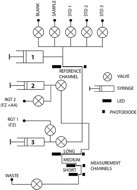
Figure 1. Schematic of the microfluidic manifold illustrating the design of the chip. Absorbance measurements are conducted in three optical cells of different length, labeled as long (91.6 mm), medium (34.6 mm), and short (2.5 mm). The syringe pumping unit comprises a large barrel (1) with 9.71 mm ID for blank, sample and standards and two small barrels (2 and 3) with 3.28 mm ID for the FZ/ascorbic acid mixture (RGT 2) and the FZ reagent (RGT 1). Solenoid valves are used for fluidic control.

The analyzer's sensitivity in laboratory based experiments was evaluated against a benchtop Agilent Cary 60 spectrophotometer using the FZ method in a 10 cm quartz cell. The absorbances at 562 nm obtained with the benchtop device were multiplied by the factor 0.916 to correct for the different cell lengths.

Chemical Assays

All glass and plastic ware was cleaned prior to use with ~2 vol% Citranox acid detergent (Sigma-Aldrich), followed by soaking in a 1.2 M HCl bath (reagent grade, Carl Roth) over night and then rinsed with de-ionized water (MilliQ, 18.2 MΩcm; Merck Millipore) at least three times. Reagents and standards were all prepared and diluted with de-ionized water, except where stated otherwise. For the detection of Fe(II) a 10 mM FZ solution (3-(2-Pyridyl)-5,6-diphenyl-1,2,4-triazine-p,p′-disulfonic acid monosodium salt hydrate, 97%; Sigma-Aldrich) was prepared with a 2 M acetate buffer (pH ~ 6) consisting of 0.1 M acetic acid (ultra purity acid grade, ROMIL) and 1.9 M sodium acetate (BioXtra, ≥99.0%, Sigma-Aldrich) giving a final concentration of 0.8 M of the acetate buffer in the FZ reagent. For analysis of DFe the FZ reagent additionally contained 0.1 M ascorbic acid (TraceSELECT, ≥99.9998%, Sigma-Aldrich) acting as a reducing agent to reduce Fe(III) to Fe(II). FZ solutions were prepared weekly and stored at 4°C in high density polyethylene (HDPE) bottles wrapped in aluminum foil to protect them from light. Ammonium iron(II) sulfate hexahydrate (99.997% trace metals basis, Sigma-Aldrich) and iron(III) chloride hexahydrate (≥98%, Carl Roth) were used to prepare 20 mM stock solutions of Fe(II) and Fe(III), respectively. These stock solutions were further diluted to 20 μM which was then used for the preparation of the Fe(II) and Fe(III) working standard solutions. All stock and working solutions were stabilized by the addition of concentrated HCl (ultra purity acid grade, ROMIL) giving a HCl concentration of ~12 mM. To prevent the Fe(II) solutions from oxidizing the standards were stabilized using 1 μM sodium sulfite (BioXtra, ≥98%, Sigma-Aldrich). Stock solutions were made fresh on a weekly basis and stored in opaque HDPE bottles at 4°C. Working standards were prepared daily for the use in the laboratory.

South Atlantic seawater ([DFe] < 0.2 nM) was used for the preparation of the blank and standard solutions for the in situ deployment (50 nM Fe(II) and 100 nM Fe(III)) and diluted with de-ionized water to obtain a salinity of 18, which approximately mimicked the conditions in the Kiel Fjord. All FZ reagents, Fe standards and the blank solution for the in situ deployment were stored in 150 and 500 mL transparent flexible bags (Flexboy-Bag, Sartorius) covered with dark tape to prevent sun light induced degradation. The bags were suspended inside a polyvinyl chloride (PVC) tube (length 440 mm, diameter 200 mm), which was attached to the top of the main analyzer housing.

Deployment Site and Discrete Sampling

As part of the SenseOCEAN EU project the Fe lab-on-chip analyzer was tested together with other microfluidic analyzers for nitrate, phosphate and pH as well as several optodes in situ in the Baltic Sea at 54°19′48.7″N 10°08′59.5″E (inner Kiel Fjord) in the period from September 12th to 20th, 2016. The inner Kiel Fjord forms the southernmost part of the Kiel Bay, is extensively used for shipping, has extensive dockyards and a population of ca 250,000 in the surrounding areas. Kiel Fjord has a mean depth of ~13 m, and a maximum tidal range of 4 cm. During the deployment a variation in water height of ±0.2 m was observed, attributed to winds and pressure gradients over the Baltic Sea. A residence time of a few days has been reported for waters in Kiel Fjord during periods with strong winds (Javidpour et al., 2009). The major source of freshwater input is rainwater from Kiel and the surrounding areas, which drains into the fjord, and the Schwentine River, located at the eastern shore of the inner Kiel Fjord.

All microfluidic analyzers and some of the optodes were electrically integrated using a central Modbus hub (Chelsea Technologies Group Ltd., UK) which logged data and provided power. All connected instruments were mounted on two stainless steel frames which were lowered from a pontoon to 2 m water depth. The frames were raised every one to two days in order to inspect the functionality of the sensor packages (e.g. bio-fouling, condition of filters etc.) and to download the data. An EXO2 sonde (YSI Inc., USA) was deployed from September 14th onwards, in order to continuously record hydrographic parameters (salinity, water temperature and oxygen saturation). Directly next to the deployment site discrete samples were collected three to four times per day using a trace metal clean 5 L GO-FLO sampling bottle (General Oceanics Inc, USA) on a nylon line at 2 m water depth. Subsampling was conducted in a clean laboratory and completed within 30 minutes of sample collection. Dissolved oxygen samples were collected in Winkler glass bottles (nominal volume of 60 mL) in duplicate and analyzed at the end of each day by Winkler titration (Carpenter, 1965). Samples for the determination of the dissolved inorganic carbon (DIC) and total alkalinity (TA) were collected in 250 mL ground-glass stoppered borosilicate bottles and spiked with 50 μL saturated HgCl₂ solution. DIC was analyzed by coulometric titration using a single-operator multiparameter analyzer (SOMMA) (Johnson et al., 1993). The TA was measured by potentiometric titration using a VINDTA 3S (Mintrop et al., 2000). Measurements were calibrated using certified reference material (batch 142) obtained from A.G. Dickson (Scripps Institution of Oceanography, USA). The in situ pH was calculated on the free scale from DIC and TA using CO2SYS (van Heuven et al., 2011). The carbonic acid dissociation constants of Mehrbach et al. (1973) refitted by Dickson and Millero (1987), the boric acid dissociation constant of Dickson (1990a), the bisulphate ion acidity constant of Dickson (1990b) and the boron-to-chlorinity ration of Lee et al. (2010) were used. DFe samples were syringe filtered through 0.45 μm PES filters, which were pre-cleaned with 1 M HCl and rinsed with de-ionized water prior to use. Samples were collected in pre-cleaned (Mucasol detergent for one day, one week in 1.2 M HCl, one week in 1.2 M HNO₃ with three de-ionized water rinses after each stage) 125 mL low density polyethylene (LDPE, Nalgene) bottles. Total dissolvable Fe (TdFe) samples were collected as per DFe samples, but without filtration. TdFe and DFe samples were then acidified to pH < 2 by the addition of 150 μL concentrated HCl (ultra purity acid grade, ROMIL) and stored for six months prior to analysis. Samples were then diluted using 1 M distilled HNO₃ (Spa grade, Romil, distilled using a sub-boiling PFA distillation system, DST-1000, Savillex), and subsequently analyzed by high resolution ICP-MS (ELEMENT II XR, ThermoFisherScientific) with calibration by standard addition. Analysis of the Certified Reference Materials NASS-7 and CASS-6 yielded Fe concentrations of 6.21 ± 0.62 nM (NASS-7, certified 6.29 ± 0.47) and 26.6 ± 0.71 nM (CASS-6, certified 27.9 ± 2.1), respectively. For the determination of dissolved organic carbon (DOC), fjord water was syringe filtered (using pre-cleaned 0.45 μm PES filters) into pre-combusted glass vials. The DOC samples were acidified to pH < 2 with 50 μL conc. HCl (trace metal grade, Carl Roth) per 20 mL seawater. DOC was then analyzed as non-purgeable organic carbon (NPOC) using a high temperature catalytic combustion approach (Shimadzu TOC-L CPH) with direct aqueous injection (Spyres et al., 2000). Meteorological data (e.g., solar irradiation, wind speed, wind direction) next to the deployment site were obtained from the GEOMAR weather station.

Results and Discussion

Laboratory Characterization

Calibration and Analyzer Sensitivity

In order to investigate the response of the in situ analyzer, calibration experiments with Fe standards of different concentrations were conducted in the laboratory (Figure 2). Molar extinction coefficients of 27,200 ± 380 L·mol⁻¹·cm⁻¹ and 22,100 ± 240 L·mol⁻¹·cm⁻¹ were obtained with the benchtop spectrophotometer (at 562 nm) and the lab-on-chip analyzer, respectively. Whilst the coefficient determined using the spectrophotometer was in close agreement with the reported value of 27900 L·mol⁻¹·cm⁻¹ (Stookey, 1970), the coefficient obtained with the in situ analyzer was notably lower (Figure 2A). This reduced sensitivity of the analyzer was most likely the result of the use of LEDs with a peak wavelength of 575 nm, whereas the absorption maximum of the Fe-(FZ)₃ complex is located at 562 nm. Nevertheless, the microfluidic Fe lab-on-chip device is able to detect Fe concentrations with a mean LOD of 1.9 nM for the long cell (calculated as three times the standard deviation of the blank, n = 23). This is significantly lower than other Fe in situ analyzers with reported LODs of 25 nM (SCANNER; Coale et al., 1991; Chin et al., 1994), 70 nM (ALCHMIST; Sarradin et al., 2005), 300 nM (CHEMINI; Vuillemin et al., 2009), and 27.25 nM (IonConExplorer; Jin et al., 2013). This enables measurements of DFe concentrations in the low nM regime typically found in coastal waters. Fe standards with concentrations higher than 5 μM exceeded the linear detection range of the long measurement cell (Figure 2B), whereas the medium cell (Figure 2B) is capable of measuring elevated Fe concentrations, up to 20 μM, with a linear response. The calibration data recorded with the short measurement cell are not presented here since the range of this cell far exceeds Fe concentrations expected in the water column. Possible applications for the short cell could be Fe analyses in sediment pore waters, where Fe concentrations in the order of several hundred μM can be found (Burdige, 1993). Due to the combined use of three different cell lengths, the analyzer is flexible with respect to deployment environments, and thus could potentially be employed in regions with high and variable Fe concentrations.

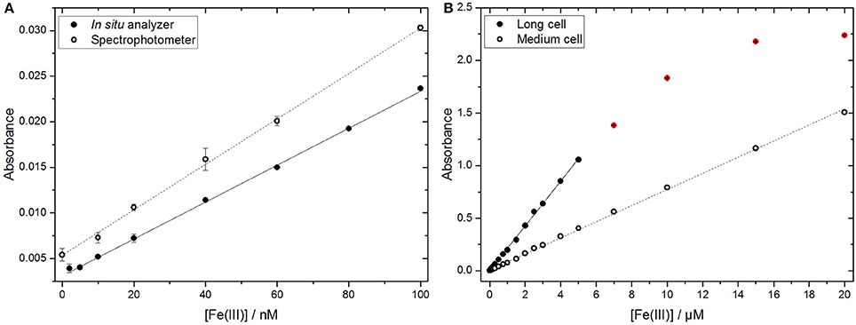
Figure 2. Calibration and detection range of the in situ analyzer. (A) Calibration curves for Fe(III) standards obtained with the long cell of the in situ analyzer produced a molar extinction coefficient of 22,100 ± 240 L·mol⁻¹·cm⁻¹ (n = 4, filled circles plotted ± standard deviation, R² = 0.999) compared to a benchtop spectrophotometer derived molar extinction coefficient of 27,200 ± 380 L·mol⁻¹·cm⁻¹ (n = 3, open circles plotted ± standard deviation, R² = 0.999). (B) The linear range for Fe detection with the long (filled circles) and medium (open circles) cells of the analyzer (n = 4), error bars are within the symbols. Data points outside the linear response are presented in red.

Flushing Procedure of Microfluidic Device

In order to minimize carry-over between standards or samples the required number of flushing steps was determined. For this purpose, the experimental routine was to flush the system first with a 1 μM Fe(II) standard and a pump stroke duration of 6 s (equivalent to 140 μL) followed by the injection with a pump stroke duration of 24 s (equivalent to 560 μL) for the final absorption measurement (red data points in Figure 3). At least two flushing steps were required to obtain a maximum absorbance signal. The system was then flushed with de-ionized water to determine the required number of flushing steps to prevent carry-over of the Fe(II) standard (blue data points in Figure 3). Five repetitions of a pump stroke with a duration of 6 s was found to be appropriate to completely flush the system of the previous solution prior to the next analysis. The flushing experiments were also performed with pump stroke durations of 12 and 24 s (280 and 560 μL, respectively). The same results were produced with all three settings. Therefore, carry-over is more dependent on the number of flushes, rather than the total flushing volume. This is likely because much of the volume that needs to be flushed is situated in the bottom of the large syringe barrel, rather than the fluidic channels of the chip. Thus, prior to each absorbance measurement (both during the deployment and the characterization in the laboratory) 5 × 6 s flushing steps were applied with the respective fluid, followed by a final injection with a pump stroke duration of 24 s for the absorbance measurements during which time the FZ reagent (56 μL) was also injected. Consequently, 1.26 mL of each blank, standard and sample and 168 μL FZ reagent were consumed for each full measurement cycle consisting of one blank, one standard and one sample analysis.

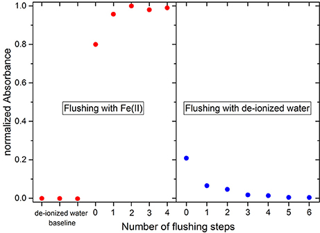
Figure 3. Required flushing steps to avoid a carry-over of reagents and standards. The x-axis shows how many flushing steps with a pump stroke duration of 6 s have been applied prior to the injection of the reagents with a pump stroke duration of 24 s for the final absorption measurements. Red data points indicate flushing and absorption measurements with a 1 μM Fe(II) standard, whereas blue data points represent de-ionized water. The first three data points refer to de-ionized water measurements and were set as 0. The maximum absorbance for the Fe(II) standard was normalized to 1.

Response Time of Analyzer

Continuous flow devices rely on turbulent mixing of reagents with blank, standard or sample solutions, which takes place in integrated mixing columns or reaction coils as in SCANNER (Chin et al., 1994) and ALCHIMIST (Sarradin et al., 2005), respectively. In contrast, the microfluidic lab-on-chip analyzer was designed as a stopped flow manifold, where the mixing of the reagent with blank, standards and sample is reliant mainly on diffusive processes, and laminar flow conditions are dominant. The results of tests to determine the required time for complete mixing at three different temperatures are shown in Figure 4. The time which defines complete mixing was calculated as τ₉₉, where the signal reached 99% of a stable photodiode output. It was assumed that the time required for full color development is limited by diffusion (seconds to minutes) rather than by the chemical reaction when an Fe(II) spike is added to a FZ solution in a de-ionized water matrix because a stable signal was obtained once mixing was completed (for t > τ₉₉). To confirm this assumption an experiment with a benchtop spectrophotometer at temperatures between 10°C and 25°C was conducted, using an Fe(II) standard manually mixed with FZ. After manual mixing, which occurred within 15 s, the absorbance was constant for all applied temperatures. Due to the inverse relationship between temperature and diffusion coefficient the mixing process in the microfluidic device at 20°C is faster than at 11°C or 6°C with τ₉₉ of 35, 50 and 55 s, respectively (Figure 4). Directly after the injection the light passing through the measurement cell was almost completely attenuated (very low signal), and the light intensity reaching the photodiode increased with time. This is because a boundary layer is generated when fluids with varying densities and refractive indices are not well mixed (the Schlieren effect). This fluidic interface can act as liquid lens resulting in a loss of light intensity along the optical path (Zagatto et al., 1990; Dias et al., 2006). The boundary layer disappears with time by diffusive mixing. However, an additional problem is raised by the speciation of Fe in natural waters where DFe will be present as organic complexes and colloids due to the presence of DOM (Gledhill and Buck, 2012). This will affect the reduction rate for DFe measurements and the kinetics of the chemical reaction between Fe(II) and FZ due to a slow release of Fe from its complexes/colloids (Box, 1984; Hopwood et al., 2014). Consequently, a waiting period of less than 1 min may be sufficient to detect only the free/unbound Fe species and may underestimate the total DFe concentration. Taking into account the above issues (temperature, the Schlieren effect, presence of DOM), a waiting period of 5 min prior to the absorption measurements during the deployment was implemented as an attempted compromise between measurement frequency and minimizing the underestimation of DFe species.

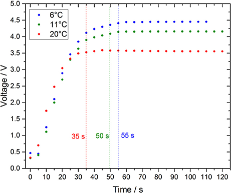
Figure 4. Required time to allow complete mixing and stable color development of a 40 nM Fe(II) standard with 10 mM FZ in a de-ionized water matrix using the long measurement cell. The raw voltage signal of the photodiode of the long cell is shown here (inversely proportional to absorbance). Response times are given as τ₉₉, when the detector output corresponds to 99% of the maximum signal. Differences in the final recorded voltage for the three applied temperatures after stable signals are obtained due to the temperature dependent signal output of the photodiodes.

Measurement Frequency and Fluid Consumption

The settings established in the previous sections (required number of flushing steps and waiting period for complete mixing/reaction) combined to a single measurement duration of ca. 7.5 min. As the deployment measurement sequence consisted of six individual measurements (2 × blank, 2 × standards, 1 × Fe(II) sample, 1 × DFe sample, see section Lab-on-Chip Analyzer Design and Specifications), one complete cycle for the in situ determination of the concentration of Fe(II) and DFe took approximately 45 min. This was a much lower measurement frequency than continuous flow analyzers can provide (e.g., 22 samples per hour for the ALCHIMIST analyzer Sarradin et al., 2005), but sufficient for the purpose of long term in situ monitoring where other constraints, such as reagent consumption, are also important design considerations. Additionally, if required, the measurement frequency of the lab-on-chip analyzer can be increased by programming the sequence such that blanks and standards are analyzed less frequently than every measurement cycle, for example once per hour, resulting in a measurement frequency of eight Fe(II) or DFe samples per hour and less fluid consumption. A major drawback of continuous flow analyzers is a limited operational lifetime due to their power and reagent consumption (Nightingale et al., 2015). For example, the ALCHIMIST analyzer consumes 36 mL sodium chloride carrier solution, 18 mL FZ reagent and 18 mL reducing agent over 45 min, or normalized per sample: 2.2 mL carrier solution, 1.1 mL of FZ reagent and reducing agent, respectively, excluding standard and blank solution (Sarradin et al., 2005). Whereas, the fluid consumption of our microfluidic approach within 45 min was approximately 2.5 mL of blank and standard solutions and approximately 170 μL of the FZ and the FZ/ascorbic acid reagent. Normalized per sample, excluding standard and blank measurements, a consumption of 56 μL of color-forming reagent follows from above. The resulting total fluid consumption for a nine day deployment was therefore a relatively modest 730 mL of blank and sample, 360 mL of each standard and 50 mL of FZ and FZ/ascorbic acid reagent.

Deployment in Kiel Fjord

Standard Stability and Time Series

For the in situ deployment of the Fe lab-on-chip analyzer two standards, 50 nM Fe(II) and 100 nM Fe(III), were used to determine the Fe(II) and DFe concentrations in Kiel Fjord. Both standards showed a very good stability with no significant drift over the nine days (Figure 5), resulting in a precision of 2.7% (n = 214) for measurements of the Fe(II) standard (black data points) and 1.9% (n = 217) for the Fe(III) standard (red data points). A linear fit according to the Beer-Lambert Law between each reagent blank and standard measurement was used to calculate the in situ concentration of Fe(II) and DFe. As shown in Figure 6, a maximum of 42 nM (September 18th, evening) and a minimum of 17 nM (September 13th, morning) was determined for Fe(II) during the nine day deployment with a mean in situ concentration of 28 ± 5 nM. The nine day mean of the DFe concentration was 39 ± 6 nM with a maximum of 57 nM (September 13th, evening) and a minimum of 27 nM (night between September 13th and 14th). Sunlight induced photochemical processes may affect the concentrations of Fe(II) and DFe, but there was no clear evidence of a diurnal trend within this data series over the whole nine deployment days. Sunlight was measured as solar irradiation with a peak irradiation of ~600 W·m⁻² (gray line, Figure 6). For the first three days of the deployment (September 13th to 15th) stable weather conditions were experienced with low cloud cover and clear water conditions with the frame visible from the pontoon in 2 m water depth. On these sunny days there is an indication for a semidiurnal trend of both Fe(II) and DFe, with increasing concentrations during the morning, maximum concentration near noon and reduced levels in the evening. These variations may be linked to photochemical processes (Weber et al., 2005; Fan, 2008). Increased concentrations during the night may be related to sediment resuspension. From September 16th to 19th it was partly cloudy, with the lowest solar irradiance recorded on September 18th. The wind direction was almost exclusively from the northeast (from the estuary of the Schwentine River heading toward the deployment pontoon) with elevated speeds up to 9 m·s⁻¹. From September 16th to 19th shallow sediments around the fjord were resuspended producing very turbid water with high light attenuation. The water temperature at 2 m depth generally showed a diurnal cycle ranging from approximately 19.5°−20.5°C daily until September 17th. A nearly constant water temperature of ~19°C was recorded for the last three deployment days. The salinity ranged from 18.6 (September 17th, noon) to 20.2 (September 19th, morning) with a mean salinity of 19.5. The calculated in situ pH ranged between 7.8 and 8.2, which is within the range expected for the Kiel Fjord in September (Wahl et al., 2015). A mean dissolved oxygen concentration of 257 μM, with a minimum of 197 μM O₂ (September 19th, morning) and a maximum of 308 μM O₂ (September 15th, afternoon) was observed for the manually collected samples. The DOC concentration showed a lower dynamic range, with DOC concentrations between 242 and 277 μM over the whole deployment.

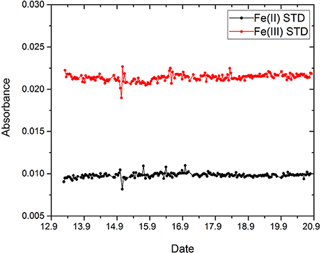
Figure 5. Stability of two Fe standard solutions, 50 nM Fe(II) (black line) and 100 nM Fe(III) (red line) over the duration of the nine day deployment in Kiel Fjord.

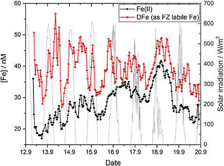
Figure 6. Nine day time series of Fe(II) and DFe (as FZ labile Fe) obtained with the in situ analyzer in Kiel Fjord together with the recorded solar irradiation (gray line) next to the deployment site.

The Spearman's rank correlation test was used to identify correlation/anti-correlation between the above mentioned variables and the in situ obtained Fe(II) and DFe concentrations. The results are summarized in Table 1, with shaded cells indicating statistically significant results (P < 0.05). A strong statistically significant anti-correlation was found between wind speed and salinity at the deployment site (P = 2.0 × 10⁻⁷). The high wind speeds produced low salinities next to the pontoon, which implies the predominance of a wind driven freshwater transport. The in situ analyzer showed increasing Fe(II) and DFe concentrations at low salinities/high wind speeds with a strong statistical significance as would generally be expected in any estuarine system with enhanced Fe levels in the freshwater end member and a loss of DFe and Fe(II), mainly via flocculation, with increasing salinity (Boyle et al., 1977; Huang et al., 2015). The in situ determined Fe(II) concentration tended to decrease with increasing oxygen saturation, measured with the probe situated next to the analyzer, with a statistical significance of P = 0.021. This is most likely because Fe(II) is thermodynamically unstable under oxic conditions and rapidly oxidized to Fe(III), with an anticipated Fe(II) half-life ranging from 0.5 to 6.2 min under the conditions measured in the Kiel Fjord (estimated using oxidation rate constants from Millero et al., 1987).

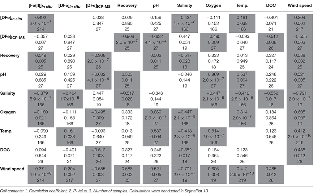
Table 1. Spearman's correlation, variables which correlate/anti-correlate (P < 0.05) are highlighted.

Evaluation of the Ferrozine Method

Despite the reasonable observed trends and correlations between dissolved Fe(II) and DFe concentrations and other hydrographic parameters, the Fe(II) fraction was unexpectedly high for oxic water conditions. A Fe(II) fraction of 45% of the total in situ determined DFe pool was observed on the first day of the deployment, rising to an average fraction of 80% for September 16th to 20th with a maximum of 97% in the evening of September 16th. Other studies report much lower fractions, ranging from 7 to 30% for estuaries using a similar FZ based method (Hopwood et al., 2015). Our elevated in situ Fe(II) fractions could be generated by either an overestimation of Fe(II) concentrations or an underestimation of DFe concentrations by the FZ based microfluidic system. An overestimation of the Fe(II) concentration may be produced by an undesired reaction of labile Fe(III) with FZ contributing to the final absorption of the colored Fe-(FZ)₃ complex (Viollier et al., 2000). It was reported that FZ tends to shift the Fe redox speciation through the reduction of Fe(III) to Fe(II), with a reaction half-time of several hours to days at pH = 5, depending on the Fe(III) and FZ concentrations (Mao et al., 2015). The sample to FZ reagent mixing ratio in the in situ analyzer produces a final pH of ~5.3. Thus, at this reaction pH and with a mixing time of only 5 min, the potential for overestimation of Fe(II) is limited. However, the rate of FZ induced Fe(III) reduction in natural waters may be accelerated in the presence of DOM (Hopwood et al., 2014).

Comparison of in situ DFe measurements with ICP-MS

To validate the in situ DFe measurements and to examine the extent of a possible underestimation, discrete samples (n = 27) were manually collected, acidified and measured via ICP-MS according to the GEOTRACES protocol for analysis of DFe concentrations in seawater. The DFe concentration of the discrete samples showed a high variability (Figure 7A) ranging from 61 nM (September 18th, noon) to 235 nM (September 19th, morning). Critically, the in situ time series and the discrete samples do not show a significant relationship (P = 0.847, see Table 1). Furthermore, in contrast to the analyzer, a strong anti-correlation between the DFe concentration of the discrete samples and the seawater pH was obtained (P = 4.1 × 10⁻⁴), which is most likely due to the removal of Fe(III) from the dissolved phase at high seawater pH values as a consequence of its precipitation as particulate Fe-oxyhydroxides (Byrne and Kester, 1976; Rose and Waite, 2003a). While the in situ measurements showed a strong anti-correlation with salinity, and a correlation with wind speed, the ICP-MS data are weakly correlated with salinity and anti-correlated with wind speed, with P = 0.054 and P = 0.003, respectively. These differences cannot be attributed to any mechanical failure of the analyzer. The lack of a relationship between DFe concentrations measured in situ and via ICP-MS strongly suggests that the analyzer does not measure some DFe species in coastal seawater using the current physical and chemical setup. While the ICP-MS analyses provided the total DFe concentration, it can be assumed that the analyzer with the setup and conditions used here only measures kinetically labile Fe species including weak complexes and colloids (Hopwood et al., 2014), where labile refers to the lability of the Fe species to the FZ/ascorbic acid reagent over a period of 5 min.

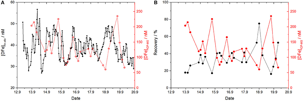
Figure 7. (A) Time series of the DFe in situ measurements (black, as FZ labile Fe) and discrete samples analyzed via ICP-MS (red). Note the different scales of the y-axes. (B) The analyzer's recovery (black) together with [DFe]_ICP−MS (red). For recovery calculations the moving average of the two closest in situ data points to each discrete sample was used.

Curiously, previous work contrasting FZ based Fe analyzers deployed in hydrothermal environments with discrete samples has not reported such underestimations. For the ALCHIMIST analyzer it is reported that the DFe concentrations obtained were in good agreement with ICP atomic emission spectroscopy (ICP-AES) measurements of the discrete samples (Sarradin et al., 2005). Similarly, excellent agreement was also reported between in situ measurements from the SCANNER analyzer and discrete samples analyzed both via graphite furnace atomic absorption spectroscopy (GFAAS) (Coale et al., 1991) and flow injection analysis (Chin et al., 1994). However, for both deployments there was a difference in the filtered size fractions. The in situ SCANNER samples were drawn through 10 μm (Coale et al., 1991) or 20 μm filters (Chin et al., 1994), whereas the discrete samples were filtered at 0.2 μm. Whether or not this difference matters depends on the size distribution of labile Fe/Fe(II) species in a specific natural water body. Where the concentration of labile Fe in the size range 0.2–20 μm is negligible compared to the Fe concentration <0.2 μm, it would be expected that a change in filtration size would not significantly affect a comparison of in situ and discrete Fe data. However, where the concentration of labile Fe in the size range 0.2–20 μm is non-negligible comparable to the concentration <0.2 μm, it is still possible that a similar Fe concentration could be obtained comparing sensor determined Fe_{<20 μm} and ICP determined Fe_{<0.2 μm}, because the sensor determined Fe_{<20 μm} is strictly the true concentration multiplied by a recovery factor (see section DFe recovery). Thus, in an environment where the analyzer design results in a recovery factor of significantly less than 100%, equivalence between sensor determined Fe_{<20 μm} and ICP determined Fe_{<0.2 μm} in isolation does not necessarily demonstrate that the sensor is producing data comparable to acidified ICP samples. Furthermore, the ALCHIMIST and SCANNER analyzers were both primarily tested in hydrothermal vent plumes where Fe speciation is very different from that expected in coastal seawater. Within the vicinity of hydrothermal vents only a small fraction of DFe is present as organically associated complexes or colloids (Bennett et al., 2008; Hawkes et al., 2013), whereas, in estuarine and near-shore coastal waters Fe speciation is dominated by interaction with DOM (Rose and Waite, 2003b; Buck et al., 2007; Gerringa et al., 2007). Thus, given the slower kinetics of the reaction between FZ and Fe-DOM species compared to the free Fe(II)/Fe(III) ions, the Fe recovery of a FZ based analyzer in estuarine or coastal seawaters may be considerably less than if the same sensor were deployed within a hydrothermal vent plume.

DFe recovery

The determined DFe concentrations of the discrete samples were used to calculate how well the in situ analyzer recovered DFe in the Kiel Fjord (Figure 7B, Equation 1).

Recoveries ranged from 16 to 75% of the total DFe pool with a correlation with Fe(II) concentrations (P = 0.005), pH (P = 0.011), DOC concentrations (P = 0.006) and wind speed (P = 0.002), and an anti-correlation with salinity (P = 0.028). As shown in Figure 7B, a high recovery is achieved for low DFe_ICP−MS concentrations, e.g., 75% for [DFe]_ICP−MS = 61 nM (September 18th, noon), and low recoveries for high DFe concentrations, e.g., 17% for [DFe]_ICP−MS = 225 nM (September 15th, morning), resulting in a very strong statistically significant anti-correlation between recovery and DFe_ICP−MS concentration (P = 2.0 × 10⁻⁷). This may be produced as a consequence of a kinetic effect, as shown in Figure 8. Here, the 5 min waiting period after reagent injection in the microfluidic manifold (to allow complete mixing of the reagent and stable color development) is shown for in situ determined DFe data points giving a high (red line) and a low recovery (black line). The mixing process of the two phases (FZ/ascorbic acid reagent and sample) was completed after 50–60 s, where both curves show the maximum light intensity reaching the photodiode detector, indicating an homogenous mixture without the presence of any measurable Schlieren effect (see section Response Time of Analyzer). After complete mixing was achieved, the intensity of the transmitted light through the long measurement cell decreased exponentially due to a progressing Fe-(FZ)₃ complex formation and thus color development. As expected, the curve for the data with a low recovery (high [DFe]_ICP−MS) had a stronger exponential decay than the data with a high recovery (low [DFe]_ICP−MS). Also, both curves continued to decrease after 300 s of the waiting period, and did not reach their final stable intensity value. This means that the selected time of 5 min to allow color development for DFe measurement is insufficient for the Fe(III) reduction/Fe-(FZ)₃ complex formation process in natural waters if Fe is present as species other than kinetically labile Fe, causing an underestimation of DFe.

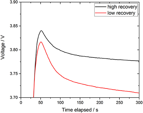
Figure 8. Raw signal during the 5 min waiting period to allow complete mixing as well as Fe(III) reduction and complexation with FZ. Data points with a high (September 18th, noon, black line) and a low recovery (September 14th, noon, red line) are shown.

Implications for Future Analyzer Designs

To improve the DFe recovery of the in situ device using the FZ method the waiting period for the color development should be prolonged to release strongly bound Fe from their complexes and to obtain a constant absorption signal. A second, and probably more analytically robust, option would be an in line acidification step according to the GEOTRACES protocol to pH < 2 prior to the injection of the FZ/ascorbic acid reagent. This would shift the Fe speciation toward truly dissolved non-complexed Fe phases (Box, 1984; Huang et al., 2015). However, for both suggested options further investigation is needed to determine whether complete recovery can be achieved within a timescale (minutes–hours) useful for in situ deployments.

Conclusions

In this study an in situ microfluidic lab-on-chip analyzer for the determination of Fe(II) and DFe in natural waters based on the FZ method was tested to determine the required number of flushing steps (5 × 6 s), required mixing time to achieve a homogenous mixture of components (less than 1 min) and LOD (1.9 nM). It was found that the analyzer was able to detect dissolved Fe species across a broad concentration range, from 1.9 nM to more than 20 μM. This facilitates in situ deployments in a broad range of marine environments including, for example, estuaries, near-shore coastal waters, benthic boundary waters and hydrothermal vent plumes. The viability of long term deployments was demonstrated by a nine day deployment in a turbid environment with continuous and successful generation of data. However, whilst both Fe(II) and DFe time series showed expected relationships to hydrographic variables such as salinity, dissolved oxygen saturation, temperature and to solar irradiation; discrete samples analyzed via ICP-MS revealed a low and highly variable recovery of DFe. A recovery between 16 and 75% attributed to an incomplete reaction between organically-complexed Fe species and the FZ/ascorbic acid reagent meant there was no statistically significant correlation between sensor derived and discrete DFe concentrations. It is therefore suggested that the current waiting period of 5 min to allow full color development is not sufficient. Such a flaw in FZ based in situ Fe analyzer designs has not previously been widely discussed, likely because similar analyzers have been primarily developed for hydrothermal vent plumes, where organic complexation is a less prominent feature of DFe speciation. Further experiments should be undertaken to investigate the viability of a longer waiting period and the addition of an acidification step to the present design of the FZ based in situ analyzer. Such improvements may facilitate reproducible DFe data in marine environments comparable to datasets obtained from manual sample collection.

Whilst this study describes an estuarine surface deployment, the lab-on-chip analyzer is based on a microfluidic platform capable of long term deployments in environments with highly variable Fe concentrations. Future work will look at validating the analyzer in a range of these environments, ranging from rivers to the deep sea.

Author Contributions

MM and AB designed and fabricated the analyzer. FG conceived and performed the experiments with AB, and led the writing of the manuscript. MH, JC, AM, and FG carried out the field work and analyzed discrete samples. EA, MM, and DC supervised the study and provided guidance throughout. All authors contributed to the interpretation of the results and writing of the manuscript.

Funding

The research leading to these results has received funding from the European Union Seventh Framework Programme (FP7/2007-2013) project SenseOCEAN under grant agreement No. 614141, and the UK NERC project DELVE (NERC grant NE/I008845/1). FG acknowledges GEOMAR and the Transatlantic Helmholtz Research School Ocean System Science and Technology (HOSST) for funding his PhD work.

Conflict of Interest Statement

The authors declare that the research was conducted in the absence of any commercial or financial relationships that could be construed as a potential conflict of interest.

Acknowledgments

We thank Chris Cardwell, John Walk, Greg Slavik, Allison Schaap, Urska Martincic, Robin Pascal, Maxime Grand and other members of the Ocean Technology and Engineering Group (OTEG) at NOC. SenseOCEAN colleagues are thanked for assistance with the sensor deployment. We finally thank the three reviewers for their constructive comments.

References

Beaton, A. D., Cardwell, C. L., Thomas, R. S., Sieben, V. J., Legiret, F.-E., Waugh, E. M., et al. (2012). Lab-on-chip measurement of nitrate and nitrite for in situ analysis of natural waters. Environ. Sci. Technol. 46, 9548–9556. doi: 10.1021/es300419u
Bennett, S. A., Achterberg, E. P., Connelly, D. P., Statham, P. J., Fones, G. R., and German, C. R. (2008). The distribution and stabilisation of dissolved Fe in deep-sea hydrothermal plumes. Earth Planet. Sci. Lett. 270, 157–167. doi: 10.1016/j.epsl.2008.01.048
Box, J. (1984). Observations on the use of iron (II) complexing agents to fractionate the total filterable iron in natural water samples. Water Res. 18, 397–402. doi: 10.1016/0043-1354(84)90146-5
Boyle, E. A., Edmond, J. M., and Sholkovitz, E. R. (1977). The mechanism of iron removal in estuaries. Geochim. Cosmochim. Acta 41, 1313–1324. doi: 10.1016/0016-7037(77)90075-8
Buck, K. N., Lohan, M. C., Berger, C. J. M., and Bruland, K. W. (2007). Dissolved iron speciation in two distinct river plumes and an estuary: implications for riverine iron supply. Limnol. Oceanogr. 52, 843–855. doi: 10.4319/lo.2007.52.2.0843
Burdige, D. J. (1993). The biogeochemistry of manganese and iron reduction in marine sediments. Earth Sci. Rev. 35, 249–284. doi: 10.1016/0012-8252(93)90040-E
Byrne, R. H., and Kester, D. R. (1976). Solubility of hydrous ferric oxide and iron speciation in seawater. Mar. Chem. 4, 255–274. doi: 10.1016/0304-4203(76)90012-8
Carpenter, J. H. (1965). The Chesapeake Bay institute technique for the Winkler dissolved oxygen method. Limnol. Oceanogr. 10, 141–143. doi: 10.4319/lo.1965.10.1.0141
Chin, C. S., Coale, K. H., Elrod, V. A., Johnson, K. S., Massoth, G. J., and Baker, E. T. (1994). In situ observations of dissolved iron and manganese in hydrothermal vent plumes, Juan de Fuca Ridge. J. Geophys. Res. 99, 4969–4984. doi: 10.1029/93JB02036
Coale, K. H., Chin, C. S., Massoth, G. J., Johnson, K. S., and Baker, E. T. (1991). In situ chemical mapping of dissolved iron and manganese in hydrothermal plumes. Nature 352, 325–328. doi: 10.1038/352325a0
Coale, K. H., Johnson, K. S., Fitzwater, S. E., Gordon, R. M., Tanner, S., Chavez, F. P., et al. (1996). A massive phytoplankton bloom induced by an ecosystem-scale iron fertilization experiment in the equatorial Pacific Ocean. Nature 383, 495–501. doi: 10.1038/383495a0
Davison, W., and Seed, G. (1983). The kinetics of the oxidation of ferrous iron in synthetic and natural waters. Geochim. Cosmochim. Acta 47, 67–79. doi: 10.1016/0016-7037(83)90091-1
Dias, A. C. B., Borges, E. P., Zagatto, E. A. G., and Worsfold, P. J. (2006). A critical examination of the components of the Schlieren effect in flow analysis. Talanta 68, 1076–1082. doi: 10.1016/j.talanta.2005.06.071
Dickson, A. G. (1990b). Standard potential of the reaction: AgCl(s) + 1/2H2(g) = Ag(s) + HCl(aq), and the standard acidity constant of the ion HSO4- in synthetic sea water from 273.15 to 318.15 K. J. Chem. Thermodyn. 22, 113–127.
Dickson, A. G. (1990a). Thermodynamics of the dissociation of boric acid in synthetic seawater from 273.15 to 318.15 K. Deep Sea Res. Part A Oceanogr. Res. Pap. 37, 755–766.
Dickson, A. G., and Millero, F. J. (1987). A comparison of the equilibrium constants for the dissociation of carbonic acid in seawater media. Deep Sea Res. Part A Oceanogr. Res. Pap. 34, 1733–1743. doi: 10.1016/0198-0149(87)90021-5
Fan, S. M. (2008). Photochemical and biochemical controls on reactive oxygen and iron speciation in the pelagic surface ocean. Mar. Chem. 109, 152–164. doi: 10.1016/j.marchem.2008.01.005
Floquet, C. F. A., Sieben, V. J., Milani, A., Joly, E. P., Ogilvie, I. R. G., Morgan, H., et al. (2011). Nanomolar detection with high sensitivity microfluidic absorption cells manufactured in tinted PMMA for chemical analysis. Talanta 84, 235–239. doi: 10.1016/j.talanta.2010.12.026
Gerringa, L. J. A., Rijkenberg, M. J. A., Wolterbeek, H. T., Verburg, T. G., Boye, M., and de Baar, H. J. W. (2007). Kinetic study reveals weak Fe-binding ligand, which affects the solubility of Fe in the Scheldt estuary. Mar. Chem. 103, 30–45. doi: 10.1016/j.marchem.2006.06.002
Gibbs, C. R. (1976). Characterization and application of FerroZine Iron reagent as a Ferrous Iron Indicator. Anal. Chem. 48, 1197–1201. doi: 10.1021/ac50002a034
Gledhill, M., and Buck, K. N. (2012). The organic complexation of iron in the marine environment: a review. Front. Microbiol. 3:69. doi: 10.3389/fmicb.2012.00069
Hawkes, J. A., Connelly, D. P., Gledhill, M., and Achterberg, E. P. (2013). The stabilisation and transportation of dissolved iron from high temperature hydrothermal vent systems. Earth Planet. Sci. Lett. 375, 280–290. doi: 10.1016/j.epsl.2013.05.047
Hopwood, M. J., Statham, P. J., and Milani, A. (2014). Dissolved Fe(II) in a river-estuary system rich in dissolved organic matter. Estuar. Coast. Shelf Sci. 151, 1–9. doi: 10.1016/j.ecss.2014.09.015
Hopwood, M. J., Statham, P. J., Skrabal, S. A., and Willey, J. D. (2015). Dissolved iron (II) ligands in river and estuarine water. Mar. Chem. 173, 173–182. doi: 10.1016/j.marchem.2014.11.004
Huang, Y., Yuan, D., Zhu, Y., and Feng, S. (2015). Real-time redox speciation of iron in estuarine and coastal surface waters. Environ. Sci. Technol. 49, 3619–3627. doi: 10.1021/es505138f
Javidpour, J., Molinero, J. C., Peschutter, J., and Sommer, U. (2009). Seasonal changes and population dynamics of the ctenophore Mnemiopsis leidyi after its first year of invasion in the Kiel Fjord, Western Baltic Sea. Biol. Invas. 11, 873–882. doi: 10.1007/s10530-008-9300-8
Jickells, T. D., An, Z. S., Andersen, K. K., Baker, A. R., Bergametti, G., Brooks, N., et al. (2005). Global iron connections between desert dust, ocean biogeochemistry, and climate. Science 308, 67–71. doi: 10.1126/science.1105959
Jin, B., Chen, Z. W., and Zhu, S. Q. (2013). Development of an in situ analyzer for iron in Deep Sea environment. Adv. Mater. Res. 694–697, 1187–1191. doi: 10.4028/www.scientific.net/AMR.694-697.1187
Johnson, K. M., Wills, K. D., Butler, D. B., Johnson, W. K., and Wong, C. S. (1993). Coulometric total carbon dioxide analysis for marine studies: maximizing the performance of an automated gas extraction system and coulometric detector. Mar. Chem. 44, 167–187. doi: 10.1016/0304-4203(93)90201-X
Johnson, K. S., Michael Gordon, R., and Coale, K. H. (1997). What controls dissolved iron concentrations in the world ocean? Mar. Chem. 57, 137–161.
Kolber, Z. S., Barber, R. T., Coale, K. H., Fitzwater, S. E., Greene, R. M., Johnson, K. S., et al. (1994). Iron Limitation of Phytoplankton photosynthesis in the equatorial Pacific-Ocean. Nature 371, 145–149. doi: 10.1038/371145a0
Laes-Huon, A., Cathalot, C., Legrand, J., Tanguy, V., and Sarradin, P. M. (2016). Long-term in situ survey of reactive iron concentrations at the Emso-Azores observatory. IEEE J. Ocean. Eng. 41, 744–752. doi: 10.1109/JOE.2016.2552779
Le Bris, N., Sarradin, P.-M., Birot, D., and Alayse-Danet, A.-M. (2000). A new chemical analyzer for in situ measurement of nitrate and total sulfide over hydrothermal vent biological communities. Mar. Chem. 72, 1–15. doi: 10.1016/S0304-4203(00)00057-8
Lee, K., Kim, T. W., Byrne, R. H., Millero, F. J., Feely, R. A., and Liu, Y. M. (2010). The universal ratio of boron to chlorinity for the North Pacific and North Atlantic oceans. Geochim. Cosmochim. Acta 74, 1801–1811. doi: 10.1016/j.gca.2009.12.027
Legiret, F. E., Sieben, V. J., Woodward, E. M. S., Abi Kaed Bey, S. K., Mowlem, M. C., Connelly, D. P., et al. (2013). A high performance microfluidic analyser for phosphate measurements in marine waters using the vanadomolybdate method. Talanta 116, 382–387. doi: 10.1016/j.talanta.2013.05.004
Luther, G. W., Shellenbarger, P. A., and Brendel, P. J. (1996). Dissolved organic Fe(III) and Fe(II) complexes in salt marsh porewaters. Geochim. Cosmochim. Acta 60, 951–960. doi: 10.1016/0016-7037(95)00444-0
Mao, Y., Zhang, M., and Xu, J. (2015). Limitation of ferrozine method for Fe(II) detection: reduction kinetics of micromolar concentration of Fe(III) by ferrozine in the dark. Int. J. Environ. Anal. Chem. 95, 1424–1434. doi: 10.1080/03067319.2015.1114107
Martin, J. H. (1990). Glacial-interglacial CO2 change: the iron hypothesis. Paleoceanography 5, 1–13. doi: 10.1029/PA005i001p00001
Mehrbach, C., Culberson, C. H., Hawley, J. E., and Pytkowicx, R. M. (1973). Measurement of the apparent dissociation constants of carbonic acid in seawater at atmospheric pressure. Limnol. Oceanogr. 18, 897–907. doi: 10.4319/lo.1973.18.6.0897
Milani, A., Statham, P. J., Mowlem, M. C., and Connelly, D. P. (2015). Development and application of a microfluidic in-situ analyzer for dissolved Fe and Mn in natural waters. Talanta 136, 15–22. doi: 10.1016/j.talanta.2014.12.045
Millero, F. J., Sotolongo, S., and Izaguirre, M. (1987). The oxidation kinetics of Fe(II) in seawater. Geochim. Cosmochim. Acta 51, 793–801. doi: 10.1016/0016-7037(87)90093-7
Mintrop, L., Perez, F. F., Gonzales-Davila, M., Santana-Casiano, J. M., and Körtzinger, A. (2000). Alkalinity determination by potentiometric titration: intercalibration using three different methods. Ciencias Mar. 26, 23–37. doi: 10.7773/cm.v26i1.573
Moore, C. M., Mills, M. M., Arrigo, K. R., Berman-Frank, I., Bopp, L., Boyd, P. W., et al. (2013). Processes and patterns of oceanic nutrient limitation. Nat. Geosci. 6, 701–710. doi: 10.1038/ngeo1765
Nightingale, A. M., Beaton, A. D., and Mowlem, M. C. (2015). Trends in microfluidic systems for in situ chemical analysis of natural waters. Sens. Actuators B Chem. 221, 1398–1405. doi: 10.1016/j.snb.2015.07.091
Ogilvie, I. R. G., Sieben, V. J., Floquet, C. F. A., Zmijan, R., Mowlem, M. C., and Morgan, H. (2010). Reduction of surface roughness for optical quality microfluidic devices in PMMA and COC. J. Micromech. Microeng. 20:65016. doi: 10.1088/0960-1317/20/6/065016
Pascualreguera, M., Ortegacarmona, I., and Molinadiaz, A. (1997). Spectrophotometric determination of iron with ferrozine by flow-injection analysis. Talanta 44, 1793–1801. doi: 10.1016/S0039-9140(97)00050-7
Prien, R. D. (2007). The future of chemical in situ sensors. Mar. Chem. 107, 422–432. doi: 10.1016/j.marchem.2007.01.014
Rérolle, V. M. C., Floquet, C. F. A., Harris, A. J. K., Mowlem, M. C., Bellerby, R. R. G. J., and Achterberg, E. P. (2013). Development of a colorimetric microfluidic pH sensor for autonomous seawater measurements. Anal. Chim. Acta 786, 124–131. doi: 10.1016/j.aca.2013.05.008
Rose, A. L., and Waite, T. D. (2003b). Kinetics of iron complexation by dissolved natural organic matter in coastal waters. Mar. Chem. 84, 85–103. doi: 10.1016/S0304-4203(03)00113-0
Rose, A. L., and Waite, T. D. (2003a). Predicting iron speciation in coastal waters from the kinetics of sunlight-mediated iron redox cycling. Aquat. Sci. 65, 375–383. doi: 10.1007/s00027-003-0676-3
Sarradin, P. M., Le Bris, N., Le Gall, C., and Rodier, P. (2005). Fe analysis by the ferrozine method: adaptation to FIA towards in situ analysis in hydrothermal environment. Talanta 66, 1131–1138. doi: 10.1016/j.talanta.2005.01.012
Sarthou, G., Bucciarelli, E., Chever, F., Hansard, S. P., González-Dávila, M., Santana-Casiano, J. M., et al. (2011). Labile Fe(II) concentrations in the Atlantic sector of the Southern Ocean along a transect from the subtropical domain to the Weddell Sea Gyre. Biogeosciences 8, 2461–2479. doi: 10.5194/bg-8-2461-2011
Spyres, G., Nimmo, M., Worsfold, P. J., Achterberg, E. P., and Miller, A. E. J. (2000). Determination of dissolved organic carbon in seawater using high temperature catalytic oxidation techniques. TrAC Trends Anal. Chem. 19, 498–506. doi: 10.1016/S0165-9936(00)00022-4
Stookey, L. L. (1970). Ferrozine—a new spectrophotometric reagent for iron. Anal. Chem. 42, 779–781. doi: 10.1021/ac60289a016
Tagliabue, A., Bowie, A. R., Philip, W., Buck, K. N., Johnson, K. S., and Saito, M. A. (2017). The integral role of iron in ocean biogeochemistry. Nature 543, 51–59. doi: 10.1038/nature21058
van Heuven, S., Pierrot, D., Rae, J. W. B., Lewis, E., and Wallace, D. W. R. (2011). MATLAB Program Developed for CO2 System Calculations. ORNL/CDIAC-105b. Carbon Oak Ridge, TN: Dioxide Information Analysis Center, Oak Ridge National Laboratory, U.S. Department of Energy.
Varney, M. S. (2000). Chemical Sensors in Oceanography. Amsterdam: Gordon and Breach Science Publishers.
Viollier, E., Inglett, P. W., Hunter, K., Roychoudhury, A. N., and Van Cappellen, P. (2000). The ferrozine method revisited: Fe(II)/Fe(III) determination in natural waters. Appl. Geochem. 15, 785–790. doi: 10.1016/S0883-2927(99)00097-9
Vuillemin, R., Le Roux, D., Dorval, P., Bucas, K., Sudreau, J. P., Hamon, M., et al. (2009). CHEMINI: a new in situ CHEmical MINIaturized analyzer. Deep. Res. Part I Oceanogr. Res. Pap. 56, 1391–1399. doi: 10.1016/j.dsr.2009.02.002
Wahl, M., Buchholz, B., Winde, V., Golomb, D., Guy-Haim, T., Müller, J., et al. (2015). A mesocosm concept for the simulation of near-natural shallow underwater climates: the Kiel Outdoor Benthocosms (KOB). Limnol. Oceanogr. Methods 13, 651–663. doi: 10.1002/lom3.10055
Weber, L., Völker, C., Schartau, M., and Wolf-Gladrow, D. A. (2005). Modeling the speciation and biogeochemistry of iron at the Bermuda Atlantic Time-series Study site. Global Biogeochem. Cycles 19, 1–23. doi: 10.1029/2004GB002340
Windom, H. L., Moore, W. S., Niencheski, L. F. H., and Jahnke, R. A. (2006). Submarine groundwater discharge: a large, previously unrecognized source of dissolved iron to the South Atlantic Ocean. Mar. Chem. 102, 252–266. doi: 10.1016/j.marchem.2006.06.016
Keywords: coastal waters, dissolved iron, ferrozine, spectrophotometry, in situ chemical analyzer, lab-on-chip, microfluidics
Citation: Geißler F, Achterberg EP, Beaton AD, Hopwood MJ, Clarke JS, Mutzberg A, Mowlem MC and Connelly DP (2017) Evaluation of a Ferrozine Based Autonomous in Situ Lab-on-Chip Analyzer for Dissolved Iron Species in Coastal Waters. Front. Mar. Sci. 4:322. doi: 10.3389/fmars.2017.00322
Received: 26 May 2017; Accepted: 26 September 2017;
Published: 12 October 2017.
Edited by:
Christel Hassler, Université de Genève, SwitzerlandReviewed by:
Andrew Rose, Southern Cross University, AustraliaManuel Dall'Osto, Institut de Ciències del Mar (CSIC), Spain
Randelle M. Bundy, University of Washington, United States
Copyright © 2017 Geißler, Achterberg, Beaton, Hopwood, Clarke, Mutzberg, Mowlem and Connelly. This is an open-access article distributed under the terms of the Creative Commons Attribution License (CC BY). The use, distribution or reproduction in other forums is permitted, provided the original author(s) or licensor are credited and that the original publication in this journal is cited, in accordance with accepted academic practice. No use, distribution or reproduction is permitted which does not comply with these terms.
*Correspondence: Felix Geißler, fgeissler@geomar.de